1. Introduction
Precision agriculture relies heavily on the ability to accurately count and locate plants in crop fields via aerial imagery. This task is crucial in optimizing the use of resources [
1], such as water [
2], fertilizers, and pesticides [
3], by targeting specific areas and reducing waste. Furthermore, accurate plant detection can aid in improving crop yields by identifying and addressing issues such as pests or diseases [
4]. Additionally, it can minimize the environmental impact of agriculture by reducing the use of chemicals and the risk of pollution [
5], ultimately enhancing food security and sustainability [
6].
However, one of the major challenges in this field is the domain gap between different crops (even of the same species), as each crop possesses its own distinct characteristics, such as leaf shape, color, light conditions, or even soil, making it difficult to generalize plant detection models from one crop to another. Traditional methods of plant detection, which require manual annotation of images, are both time-consuming and costly due to the labor-intensive nature of the process, the need for a large number of labels, and the risk of error and inconsistency. Furthermore, current approaches do not account for the domain gap, necessitating the generation of a dataset that encompasses all possible domains, thus increasing the cost significantly.
This study tackles the challenge of accurate plant counting and localization in crop fields despite domain shifts by introducing a new semi-supervised method. Our approach represents a breakthrough over previous methods, as it utilizes dot annotations instead of bounding boxes, thus decreasing the cost of labeling and enabling the use of unlabeled data from new unseen shifted domains in an unsupervised manner. Our method generalizes to new domains by utilizing only unlabeled data. The approach comprises two key mechanisms: (1) unsupervised adversarial domain alignment of intermediate features and (2) self-supervision on the target domain through the inclusion of a novel pseudolabeling loss.
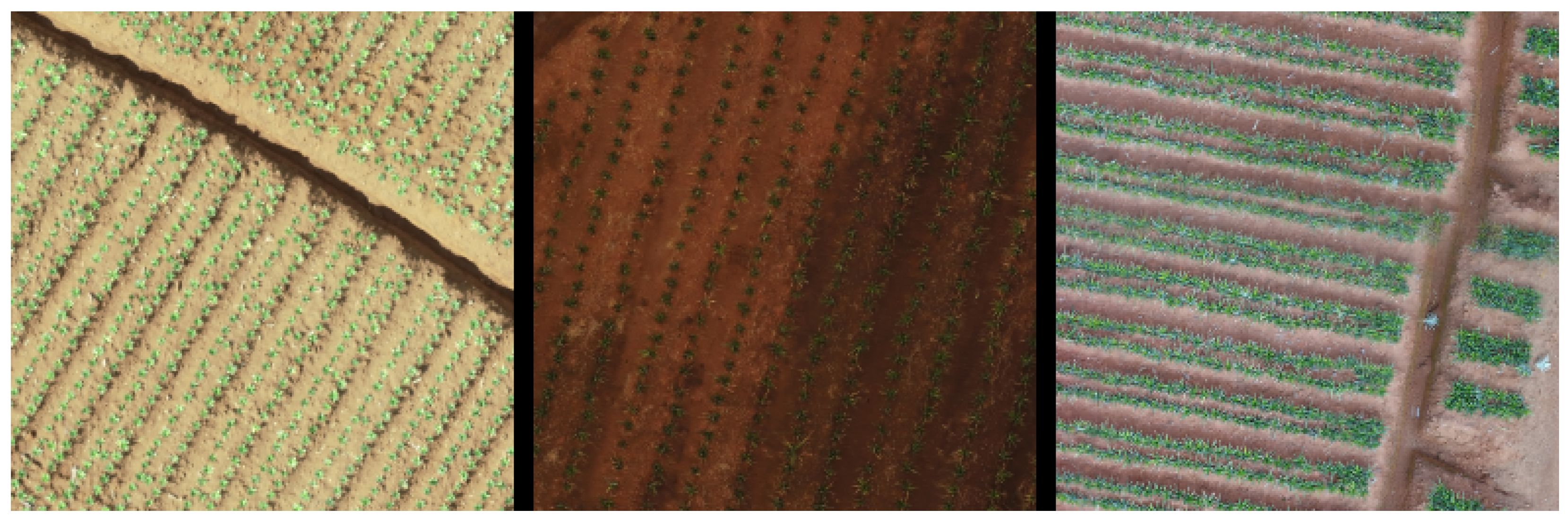
To validate the effectiveness of our system, we conducted several experiments on a dataset of pineapple crops that we created, which is composed of multiple sub-datasets, each representing a crop from a distinct geographical region. As depicted in
Figure 1, there is a striking domain shift between datasets due to factors such as lighting conditions, growth stage, soil type, etc., which makes generalizations from one dataset to another extremely challenging with traditional fully-supervised methods. To the best of our knowledge, this research is the first to tackle the problem of plant detection using dot annotations in a semi-supervised manner while addressing domain shifts. To gauge the impact of our contributions, we compared the proposed method with a fully-supervised baseline method that only utilizes the available labels as input. Our approach demonstrates a significant enhancement in localization and counting accuracy on the target domain.
In the forthcoming sections, we will first review the related literature in the field of crop counting and localization from aerial imagery. Following that, we will elaborate on our proposed approach in detail, including the network architecture and semi-supervised training procedure. We will then demonstrate the efficacy of our approach through the results of our experiments, which exhibit its versatility across a diverse range of crops and conditions. Finally, we will conclude with a discussion of the implications of our work and potential avenues for future research. Our key contributions include (1) the introduction of a novel counting method from aerial images using dot annotations, and its application to precision agriculture, (2) the presentation of an unsupervised domain adaptation method, which enables the model to leverage information from unlabeled domains to improve its generalization capabilities, and (3) the proposal of a new research direction on semi-supervised methods for crop counting robust to domain gaps, to reduce costs in agriculture.
2. Related Work
2.1. Crop Monitoring Using Aerial Images
Crop monitoring is a vital aspect of precision agriculture, and with the advent of deep learning, it has become increasingly efficient and accurate. Unmanned aerial vehicles (UAVs) have played a crucial role in crop monitoring [
7], providing high-resolution images and enabling fastmonitoring of crops [
8]. Using UAVs equipped with different cameras, such as RGB, thermal, and hyperspectral cameras, has opened up new possibilities for crop monitoring.
RGB cameras are the most widely used cameras for crop monitoring [
9,
10], providing high-resolution images that are useful for identifying plant growth stages, identifying pests and diseases, and estimating crop yield. Thermal cameras, on the other hand, can detect temperature variations in the crop canopy, providing useful information about plant stress [
11] and water uptake [
12]. Hyperspectral cameras, which can capture images across a wide range of wavelengths, can provide detailed information about the chemical composition of crops, such as chlorophyll content and water content [
13].
The utilization of deep learning models in crop monitoring has been widespread, with object detection and semantic segmentation being the most prevalent approaches. Research has been conducted utilizing object detection to identify individual plants in various crops, such as mango [
14,
15], banana [
16] or citrus tree [
17,
18]. Object detection models, such as YOLO [
19], require input data in the form of large sets of bounding boxes. While these datasets are relatively inexpensive to acquire, using dot annotations and only labeling the center of the object can reduce the amount of input data required by half. In contrast, semantic segmentation approaches enable the segmentation of pixels into different regions, such as leaves, stems, and background, providing detailed information about the structure of the crop [
20,
21,
22]. However, it is worth noting that datasets for semantic segmentation are very expensive. Generative Adversarial Networks (GANs) have a broad range of applications in agriculture, including image augmentation and synthesis, which can enhance model performance and decrease manual labor required for data preparation. GANs have already been utilized in various agricultural tasks such as plant health monitoring [
23], weeds detection [
24], or fruit inspection [
25].
2.2. Object Counting from Dot Annotations
The task of accurately counting objects within images can be approached through a variety of methods, including individual object detection [
26], direct count estimation [
27], and the generation of intermediate density maps. Our approach aligns with the method of individual object detection as proposed by [
26], as it allows for the preservation of object position information. This is achieved by generating a proximity map of each pixel to the center of the objects, utilizing dot annotations placed near the centers.
Recent advancements in object counting methods have emphasized the utilization of density map estimation, first introduced by [
28]. This approach utilizes linear regression on SIFT (Scale Invariant Feature Transform) [
29] features to estimate the density map of the desired objects. Subsequent developments in this line include the implementation of regression forests in place of linear regression [
30], modification of the data generation procedure [
31], or the application of postprocessing techniques to eliminate low confidence detections [
32].
The application of convolutional neural networks for the estimation of density maps was first introduced in [
33] as a means of circumventing the need for handcrafted features. Building upon this concept, the method proposed in [
34] incorporates a redundant counting technique by utilizing square kernels, enabling neurons to count the number of objects within their receptive field.
Recent progress in object counting has also been made through modifications to neural network architecture, such as the introduction of upsampling layers for enhanced counting resolution and improved centroid localization, as proposed by [
35]. Additionally, techniques such as those employed by [
36,
37] address the challenge of varying object sizes by implementing multiresolution methods. Furthermore, ref. [
38] proposed a channel attention module, adaptable to a wide range of neural networks, that enhances counting accuracy.
Efforts have also been made to address the challenge of errors arising from uniform background regions in object counting, such as incorporating self-attention modules [
39], background segmentation [
40,
41], or designing region-based loss functions that specifically consider background regions [
42].
2.3. Unsupervised Domain Adaptation
Unsupervised domain adaptation addresses the challenge of applying a model trained on a specific source distribution to a related but distinct target distribution. While traditional “shallow” domain adaptation methods focus on reweighting source samples and learning a shared feature space between the source and target datasets [
43], the utilization of deep neural networks (DNNs) in deep domain adaptation has proven to yield more transferable representations. This is due to the tendency of DNNs to learn highly transferable features in the lower layers, with decreasing transferability in higher layers. Therefore, the goal of deep domain adaptation is to leverage this property of DNNs.
One popular approach to deep domain adaptation is the Deep Adaptation Network (DAN) [
44], which utilizes weighting techniques to match the different domain distributions and improve feature transferability. Additionally, DAN employs an optimal multi-kernel selection method to reduce domain discrepancy further.
Another approach, Deep CORAL (Deep Correlation Alignment) [
45], is an unsupervised method that utilizes a non-linear transformation to align the correlations of layer activations in DNNs. The use of a non-linear transformation in Deep CORAL enables the capturing of complex relationships between layers, resulting in improved performance compared to linear transformations used by other methods.
Deep domain confusion [
46] is a technique for creating a representation that is both semantically meaningful and invariant across different domains. This is achieved by introducing an adaptation layer into the CNN architecture and implementing an additional loss function referred to as “domain confusion loss”. This allows the model to learn representations that are not biased towards any particular domain, making it more generalizable when applied to new contexts.
Another promising approach is CoGAN (Coupled Generative Adversarial Networks) [
47], which can learn a joint distribution of multi-domain images without requiring tuples of corresponding images in different domains in the training set. To accomplish this, CoGAN uses samples drawn from the marginal distributions and enforces a weight-sharing constraint to favor the joint distribution solution over the product of marginal distributions.
Finally, the DANN (Domain Adaptive Neural Networks) method [
48] works by augmenting a feed-forward model with standard layers and a novel gradient reversal layer. This enables the model to learn deep features that are both specific to the source domain and applicable to the target domain. The gradient reversal layer promotes adaptation behavior, allowing for successful transfer across different domains when trained using standard backpropagation.
3. Method
3.1. Overview
Our proposed method for crop counting and localization from aerial imagery comprises two distinct stages: (1) A convolutional neural network (CNN) is utilized to predict the probability of the presence of the center of each plant in the input image, and (2) a blob detector is employed to localize each plant.
To address the challenge of domain shifts between different crops, we propose a semi-supervised training procedure incorporating two key mechanisms: an adversarial framework and pseudolabeling. In the adversarial framework, we utilize a domain discriminator () to learn to differentiate between samples from two datasets that are similar but diverge due to domain shifts (e.g., different soils, growth stages of plants, lighting conditions, etc.). This forces the main network only to utilize relevant features that are present in both domains, aligning the intermediate feature representations of both domains.
However, this approach only focuses on making the domains indistinguishable at the feature level, which could result in the loss of semantic information in the target data. To circumvent this, we introduce a pseudolabeling mechanism that reinforces the confident outputs of the network and prevents forgetting as training progresses. This enables us to incorporate samples from a different source domain during training in an unsupervised manner while still preserving the semantic information present in the target domain.
3.2. Supervised Baseline Model
We adopt the methodology presented in [
49] as our supervised baseline. This approach seeks to achieve the count and localization of objects by dividing the problem into two primary stages.
Initially, a DNN G maps the input image I to a new image C, representing the probability of the presence of the center of an object at each pixel. To aid in this objective, a second neural network is utilized to discriminate between ground truth target images and those generated by G through an adversarial training procedure.
Subsequently, each individual object is detected using the Laplacian of Gaussian (LoG) [
50], enabling the detection of objects that are very close or even overlapping.
The following sections provide a more comprehensive understanding of the baseline method and the modifications we have made to it. For a thorough overview of the method, we direct the reader to the original publication [
49].
3.2.1. Target Label Construction
The aim of the generator network
G is to learn to create a map that shows the probability of finding the center of an object at each pixel of the image. This is done by defining a Gaussian map
for each pixel
x using the following equation.
where
P is the set of point annotations in the image, and
is a configurable parameter that determines the width of the blobs in the map. To calculate
, we need first to calculate the distance transform
of the annotation set:
This map represents the distance of each pixel
x to the closest point
y from the annotated set
P. We use the Euclidean distance to calculate the distances:
To avoid detecting objects that are too close together as a single one, we emphasize the frontiers between objects by setting the values of those pixels to 0. This is done using the following equation:
where
is a distance threshold that determines the thickness of the frontiers, and
and
are annotations in
P. After conducting a series of experiments, it was determined empirically that a threshold of 2 was the most effective value. Therefore, this threshold was set for all experiments. The use of these frontiers encourages the neural network to learn to divide objects that are too close together into different blobs, making detection easier.
3.2.2. Network Architecture
The baseline method uses a generative adversarial network (GAN) architecture to avoid blurry results when minimizing the Euclidean distance between pairs of pixels [
51]. The GAN consists of two networks: a generator
G that learns to map input images to intermediate representations and a discriminator
that learns to distinguish between the generated outputs from
G and the ground truth. The generator and discriminator compete with each other in an adversarial fashion, with the generator trying to produce outputs that are indistinguishable from the ground truth and the discriminator trying to identify the generated outputs accurately. This competition drives both networks to improve, ultimately resulting in more accurate center maps.
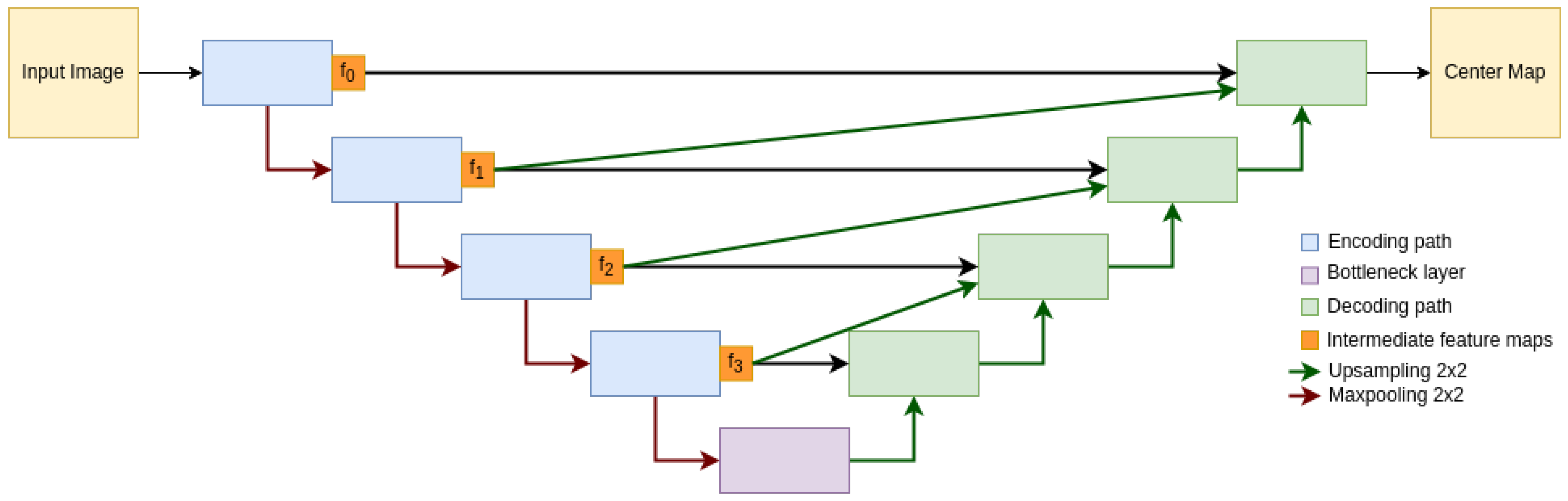
We use a modified Up-net [
49] architecture as the generator network. This design is based on the work presented in [
52] and combines the advantages of U-net [
53], and fully convolutional networks (FCNs) [
54]. U-nets are effective at extracting rich semantic features at the bottleneck layer and recovering high-frequency information at higher layers using skip connections, while FCNs use skip connections to propagate information throughout the network without increasing the total number of parameters. By combining these two approaches, our modified U-net architecture can extract useful features from the input image and reconstruct it accurately without significantly increasing the number of parameters in the network. The architecture is shown in
Figure 2The discriminator architecture follows the PatchGAN [
51] design, as outlined in
Table 1. By analyzing patches of the input image rather than the entire image, the network can lower computational costs and improve efficiency.
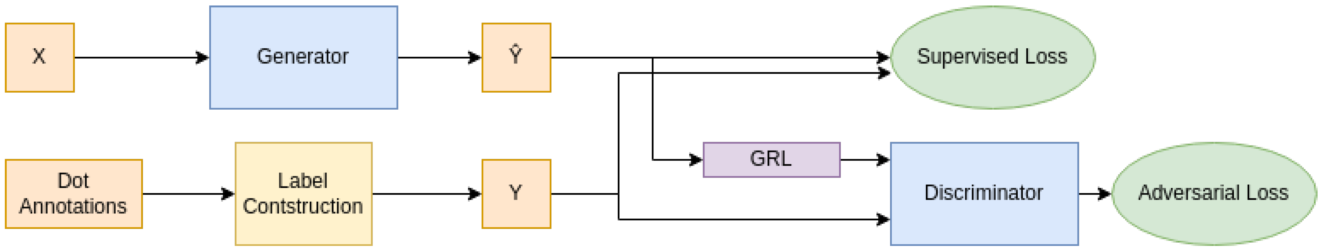
Inspired by the work of Ganin et al. [
48], we added a gradient reversal layer (GRL) between the generator and the discriminator. This change allows us to train both networks jointly in the same forward pass, reducing the training complexity and computational costs while maintaining opposing objectives in each network. As proposed in [
48], we scale the gradients flowing from the discriminator to the generator inversely proportional to the current training step to overcome the early instabilities of adversarial training.
Figure 3 provides a visual overview of the training procedure.
During training, the generator and discriminator networks are optimized using a combination of adversarial and reconstruction losses (Equations (
5) and (
6)). The adversarial loss is used to encourage the generator to produce outputs that are indistinguishable from the ground truth, while the reconstruction loss is used to encourage the generator to reconstruct the input image accurately. We adopted a least square GAN [
56] objective. These losses are combined and used to update the weights of the generator and discriminator networks, ultimately leading to more accurate results. The parameter
acts as a weighting factor between both loss terms.
3.3. Semi-Supervised Training under Domain Distribution Shifts
In this work, we aim to address the challenge of domain shift and improve the generalization of a base model by incorporating unlabeled data from the target domain into the training process. To achieve this, we propose a novel approach that combines two key mechanisms: adversarial alignment of intermediate features between the two domains and pseudo-labeling of the target domain data. Our adversarial alignment strategy involves training a neural network to perform a task while also learning domain-invariant features through an adversarial training process. This helps the model generalize better to the target domain by learning common features across both domains. Our pseudo-labeling approach involves using the model’s own predictions as labels for the target domain data, thereby preserving the richness and meaning of the target domain features and allowing the model to capture the unique characteristics of the target domain. By combining these two mechanisms, we can improve the performance of the base model on the target domain, enabling it to generalize to new domains.
3.3.1. Multilevel Adversarial Domain Align
To improve the generalization of our base model to the target domain, we draw inspiration from the DANN method [
48]. This method involves training a secondary neural network, called the domain discriminator (
), to distinguish between samples from the source and target domains based on the intermediate feature representation produced by the main network. The main network is then trained in an adversarial manner, using the gradients from the domain classification loss to update the network weights and force the encoder path to extract features that are invariant across domains.
However, in our case, we are using a U-Net-like architecture with skip connections. Enforcing feature invariance at a single point (e.g., at the bottleneck layer) is insufficient for aligning the feature spaces of the two domains due to the flow of information between different levels of the network-enabled by the skip connections. To address this issue, we propose a new multilevel domain discriminator that takes as input the features at each skip connection level, aligning the domains at each level and ensuring that all features used by the decoder path are aligned.
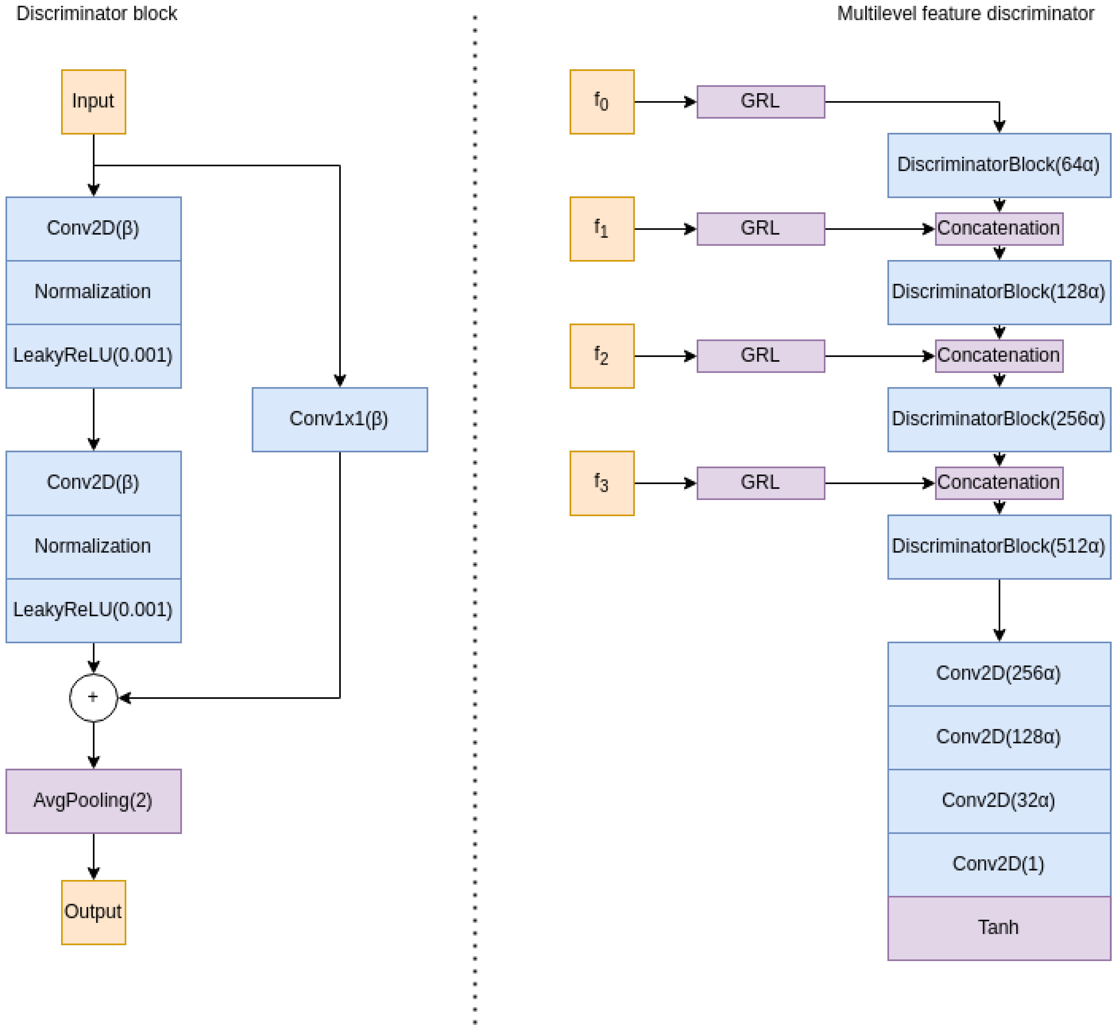
Our multilevel discriminator architecture consists of four discriminator blocks and a final block, as illustrated in
Figure 4. Each discriminator block takes as input the features at the current level, as well as the output of the previous block (except for the first block). This hierarchical representation of the features allows the network to extract and combine features at each skip connection level, enabling more effective alignment of the feature spaces of the two domains. The final block of the discriminator aggregates all of this information and uses it to determine, at the patch level, whether the features are from the source or target domain, following the PatchGan architecture proposed in [
51]. Additionally, we have added residual connections [
57] to improve the propagation of gradients and facilitate the training process.
We denote the domain label d as an indicator, with indicating that a sample is drawn from the source domain and indicating that it is drawn from the target domain.
To train the domain discriminator, we follow the Least Squares Generative Adversarial Network (LSGAN) [
56] objective, which leads to the following loss term:
Here,
E represents the encoder part of the generator network
G, as shown in
Figure 2. The domain discriminator
takes as input the intermediate feature representation at all skip levels produced by the encoder
E and produces a prediction of the domain label
d for that sample.
3.3.2. Selective Confidence Pseudolabeling
While adversarial alignment can ensure the statistical alignment of intermediate features, it does not guarantee semantic alignment. As a result, it is possible that the resulting intermediate representations in the target domain, while conforming to the same data distribution as the source domain, may not be useful for detecting plants.
To address this issue, we observed that at the early stages of training, when the network is not fully adapted to the source domain, it outputs some highly confident predictions that are accurate. However, as training progresses, the network becomes better suited to the provided data and forgets these confident outputs, resulting in an inability to detect any of the plants in the target data. To capitalize on this phenomenon, we have developed a selective confidence pseudolabeling technique to avoid forgetting these early accurate outputs.
To compute the pseudolabel, we first gather the confident coordinates. This is achieved by smoothing the network output, , with a Gaussian filter and then identifying local maxima in the output. We only consider highly confident outputs with two thresholds: an adaptive threshold , set at 0.9 of the maximum value of the current output, and a hard absolute threshold , typically set at 0.5. Additionally, we filter out maxima that are too close together using a threshold , set at , where is a configurable parameter determining the size of the blobs in the baseline method. The pseudolabel is then computed using only these dot annotations, similar to the baseline method.
Since the network does not detect all objects at the beginning of training, we do not want to train the network using negative pseudolabels. To address this, we mask the loss in pixels where the pseudolabel is less than a threshold , typically set at 0.2. Finally, we compute the loss between and the pseudolabel using an (MSE) loss.
To further improve the robustness of our approach, we use an adaptive scaling term, , to multiply the loss term. This term is scheduled to be very small at the beginning of training and gradually increases as training progresses. This helps to better gather confident pseudolabels as the network becomes more confident.
Overall, our masked selective confidence pseudolabeling approach allows us to leverage the confident outputs of the network at the early stages of training and avoid forgetting these outputs as training progresses. This helps to improve the semantic alignment of the intermediate representations in the target domain and improves the ability of the network to detect plants in the target data.
Being
the pseudolabel generated by Algorithm 1.
| Algorithm 1 Proposed selective confidence pseudolabeling |
- 1:
procedure ComputePseudoLabel() - 2:
- 3:
- 4:
- 5:
- 6:
- 7:
return - 8:
end procedure
|
4. Results
In the following section, we present the results obtained from validating our proposed method.
4.1. Experimental Setup
All the proposed method is implemented using the frameworks Pytorch [
58] and Pytorch Lightning [
59]. The GPU used for training has been an Nvidia GeForce RTX 2080 Ti. For training all networks, we use Adam [
60] optimizer with a
learning rate.
To increase the generalization capabilities of the model, we use RandAugment [
61] with 3 steps in all tests.
Dataset
In this study, we employ an aerial imagery dataset of pineapple crops from various geographical regions to demonstrate the effectiveness of our proposed method in handling domain shifts. The dataset comprises a diverse set of images that exhibit significant variations in lighting conditions, plant growth stage, soil type, and other factors. It comprises several sub-datasets, each belonging to a crop from a different geographical area, as illustrated in
Figure 1.
The images in the dataset were labeled using dot annotations, which mark the center of each plant. In total, the dataset comprises 2944 images, with a total of 33,280 plants. The images have a resolution of 256 × 256 pixels and are in the RGB color space.
To evaluate the effectiveness of our proposed method, we divided the dataset into three domain folds: A, B, and C. Each fold corresponds to a single crop with distinct characteristics. This enabled us to assess the generalization ability of our method across different domains. Folds A and B are roughly the same size, with 1408 and 1280 images, respectively, while fold C contains only 256 images. This imbalanced distribution allows us to test the robustness of our method against uneven domain sizes.
Furthermore, we have gathered a separate dataset specifically for testing the domain generalization abilities of our system. This dataset comprises data from 9 distinct domains (from different geographical areas), each with a unique set of characteristics, such as color, soil type, illumination, etc. To ensure a thorough evaluation, we have gathered a total of 4224 images across all domains, reserving 64 from each domain for testing purposes. Although the test dataset is balanced, the training dataset is strongly unbalanced across domains, with domains represented as low as 3% while others account for 20% of the representation, conforming to an additional challenge. In total, this dataset comprises 45,782 plants.
Figure 5 depicts a sample of the dataset.
4.2. Experiments
In this study, we aimed to investigate the impact of each component of our proposed method for domain adaptation in aerial images of pineapple crops. To evaluate the performance of our method, we selected the relative Mean Absolute Error (rMAE) of crop count estimates as the evaluation metric. The rMAE is defined as the ratio of the absolute error to the true count (presented in percentage). For each trial, we randomly selected 70% of the dataset for training and validation and used the remaining images as the test set. To estimate the mean and standard deviation of the rMAE, we repeated this procedure ten times.
4.2.1. Ablation Study
We conducted an ablation study to understand the individual contributions of each component of our method to the final performance. Our ablation study consisted of five experimental trials in which we systematically introduced and removed components of our method. The results of the ablation study are presented in
Table 2. The first experiment employed the baseline method without any additional modifications. In the second experiment, we introduced the adversarial domain alignment mechanism and observed an improvement in performance on the target domain. However, we encountered convergence issues when training both discriminators simultaneously, so in the third experiment, we disabled the adversarial branch of the baseline method to investigate its impact. The fourth experiment examined the pseudo-labeling approach without any domain alignment, and we observed that the pseudo-labeling approach relies on accurate and confident network outputs. Without domain alignment, the model began to reinforce incorrect pseudo-labels, leading to a significant decrease in performance. Finally, in the fifth experiment, we incorporated both pseudo-labeling and domain alignment mechanisms and observed a significant reduction in error.
4.2.2. Domain Adaptation Experiments
We also evaluated the domain adaptation capabilities of our method by testing the adaptation from one source domain to another. For this evaluation, we utilized datasets A, B, and C and compared the results of our proposed approach to those of two fully-supervised methods: a baseline method that can only access source domain labels and an oracle method that had access to both source and target domain labels. The oracle method aims to provide an expected behavior of the model when all the labels are provided, giving a sense of the magnitude of the performance increase.
Table 3 summarizes the results of our domain adaptation experiments. The results illustrate that our method consistently demonstrates proficiency in adapting between domains, resulting in a mean reduction in error up to 97%. However, there was a single instance (when the source dataset was the smallest one) where the reduction in error was limited to 10% only. Nonetheless, when our method successfully performed the adaptation, the error margins were closely aligned with those of the oracle method.
4.2.3. Domain Generalization Experiments
To measure the ability of our method to generalize across various domains at the same time, we performed experiments that evaluated its performance on the whole domain generalization dataset, each time with a different source domain A, B, and C. The results of these experiments are summarized in
Table 4. Our findings indicate that while our unsupervised approach consistently outperforms the supervised baseline, achieving a mean reduction in error of 61%, there is still room for improvement in this setting if we compare the results obtained with the oracle.
5. Discussion
In this study, we present a novel semi-supervised approach for precise plant counting in aerial images of crop fields, which effectively addresses the challenge of domain shift between training and test data commonly faced in agricultural applications. Our method integrates deep learning and domain adaptation techniques to adapt a model trained on a labeled source dataset to an unlabeled target dataset through unsupervised domain alignment and pseudo-labeling. This makes our approach highly desirable for real-world applications where labeled data may be scarce.
The experimental results show that our approach excels in handling significant domain shifts in a one-to-one adaptation setting, reducing error by up to 97% compared to a supervised baseline, remaining very competitive with respect to an oracle model with access to all labels. However, the reliance on a confidence-based pseudolabeling approach can fail when the domain gap is significant. In such cases, false positive pseudolabels can cause the model to diverge in the target domain, leading to an inability to recover. To overcome this limitation, developing mechanisms to detect such cases could be beneficial. In the domain generalization setting, our approach reduces error by an average of 61%, but there is still room for improvement as the gap with respect to oracle remains large. The confidence-based pseudolabeling approach can lead to early, confident outputs dominating the adaptation, resulting in the underrepresentation of domains with large distances from the main domain. To address this, redesigning the adversarial framework to consider multiple target domains or creating subdomains in an unsupervised manner could detect underperforming domains and increase the weight of such domains to alleviate the underrepresentation issue.
Future work in this field could address the limitations identified in this study. One approach could be to enhance the pseudolabeling mechanism to ensure more accurate label predictions and prevent model divergence in the target domain. This could be achieved by implementing voting systems for pseudolabels or incorporating a history of pseudolabels. Another area for improvement is the adaptation framework, which could be modified to consider multiple target subdomains to handle diverse domains better.
Additionally, developing unsupervised techniques for early stopping and hyperparameter tuning would be beneficial, as these mechanisms currently rely on access to target validation data. The current method also requires retraining from scratch for every new domain and access to the source dataset. To overcome these limitations, exploring source-free retraining methods that only require access to target data samples and developing online domain adaptation techniques to adapt to new domains without the need for retraining continuously would be valuable avenues for future research. Another possible avenue for future research is to improve the performance of the proposed model to enable its deployment onboard for online inspection, as its current real-time capabilities are limited when using a desktop GPU.
6. Conclusions
In conclusion, our novel semi-supervised approach is a significant improvement for plant counting in aerial images of tropical crops. It effectively addresses the challenge of domain shift by combining deep learning and domain adaptation techniques through unsupervised domain alignment and pseudo-labeling. The results of our experiments demonstrate the potential of our approach in reducing error up to 97% compared to a supervised baseline and remaining competitive with respect to an oracle model with access to all labels.
Our approach can potentially improve efficiency and sustainability in the agricultural sector, reducing the cost of crop monitoring and minimizing the use of resources such as water, fertilizers, and pesticides. However, some limitations must be addressed, such as the reliance on confidence-based pseudolabeling and the need for retraining for each new domain.
The findings of this paper provide a solid foundation for further research and have the potential to have a significant positive impact on the efficiency and sustainability of agricultural operations. To facilitate building upon our work and encourage further research in this area, we are releasing the code used in this paper. The code can be accessed at
https://github.com/cvar-upm/tropical_plant_counting_UDA.
Author Contributions
Conceptualization, J.R.-V., M.M. and P.C.; methodology, J.R.-V.; software, J.R.-V., D.P.-S. and M.F.-C.; validation, D.P.-S. and M.F.-C.; formal analysis, J.R.-V. and D.P.-S.; investigation, J.R.-V.; resources, P.C.; data curation, D.P.-S. and M.F.-C.; writing—original draft preparation, J.R.-V.; writing—review and editing, D.P.-S., M.F.-C., M.M. and P.C.; supervision, M.M. and P.C.; project administration, P.C.; funding acquisition, P.C. All authors have read and agreed to the published version of the manuscript.
Funding
This work has been supported by the project COPILOT ref. Y2020/EMT6368 “Control, Monitoring and Operation of Photovoltaic Solar Power Plants using synergic integration of Drones, IoT, and advanced communication technologies”, funded by the Madrid Government under the R&D Synergic Projects Program and partially funded by the project INSERTION ref. ID2021-127648OBC32, “UAV Perception, Control and Operation in Harsh Environments”, funded by the Spanish Ministry of Science and Innovation under the program ”Projects for Knowledge Generation”. The work of the third author is supported by the Spanish Ministry of Science and Innovation under its Program for Technical Assistants PTA2021-020671.
Data Availability Statement
Not applicable.
Acknowledgments
The authors would like to thank Indigo Drones for proving the aerial images for this study and to Adrián Álvarez-Fernández and Joaquín Fernández-Zafra for helping in the labeling process of the dataset.
Conflicts of Interest
The authors declare no conflict of interest.
References
- Bongiovanni, R.; Lowenberg-DeBoer, J. Precision agriculture and sustainability. Precis. Agric. 2004, 5, 359–387. [Google Scholar] [CrossRef]
- Lu, Y.; Liu, M.; Li, C.; Liu, X.; Cao, C.; Li, X.; Kan, Z. Precision Fertilization and Irrigation: Progress and Applications. AgriEngineering 2022, 4, 626–655. [Google Scholar] [CrossRef]
- Talaviya, T.; Shah, D.; Patel, N.; Yagnik, H.; Shah, M. Implementation of artificial intelligence in agriculture for optimisation of irrigation and application of pesticides and herbicides. Artif. Intell. Agric. 2020, 4, 58–73. [Google Scholar] [CrossRef]
- Li, W.; Chen, P.; Wang, B.; Xie, C. Automatic localization and count of agricultural crop pests based on an improved deep learning pipeline. Sci. Rep. 2019, 9, 7024. [Google Scholar] [CrossRef] [Green Version]
- Roberts, D.P.; Short, N.M.; Sill, J.; Lakshman, D.K.; Hu, X.; Buser, M. Precision agriculture and geospatial techniques for sustainable disease control. Indian Phytopathol. 2021, 74, 287–305. [Google Scholar] [CrossRef]
- Cohen, A.R.; Chen, G.; Berger, E.M.; Warrier, S.; Lan, G.; Grubert, E.; Dellaert, F.; Chen, Y. Dynamically Controlled Environment Agriculture: Integrating Machine Learning and Mechanistic and Physiological Models for Sustainable Food Cultivation. ACS ES&T Eng. 2021, 2, 3–19. [Google Scholar]
- Barbedo, J.G.A. A review on the use of unmanned aerial vehicles and imaging sensors for monitoring and assessing plant stresses. Drones 2019, 3, 40. [Google Scholar] [CrossRef] [Green Version]
- Hafeez, A.; Husain, M.A.; Singh, S.; Chauhan, A.; Khan, M.T.; Kumar, N.; Chauhan, A.; Soni, S. Implementation of drone technology for farm monitoring & pesticide spraying: A review. Inf. Process. Agric. 2022. [Google Scholar] [CrossRef]
- Bouguettaya, A.; Zarzour, H.; Kechida, A.; Taberkit, A.M. A survey on deep learning-based identification of plant and crop diseases from UAV-based aerial images. Clust. Comput. 2022, 26, 1297–1317. [Google Scholar] [CrossRef] [PubMed]
- Bouguettaya, A.; Zarzour, H.; Kechida, A.; Taberkit, A.M. Deep learning techniques to classify agricultural crops through UAV imagery: A review. Neural Comput. Appl. 2022, 34, 9511–9536. [Google Scholar] [CrossRef]
- Pineda, M.; Barón, M.; Pérez-Bueno, M.L. Thermal imaging for plant stress detection and phenotyping. Remote Sens. 2020, 13, 68. [Google Scholar] [CrossRef]
- Stutsel, B.; Johansen, K.; Malbéteau, Y.M.; McCabe, M.F. Detecting plant stress using thermal and optical imagery from an unoccupied aerial vehicle. Front. Plant Sci. 2021, 12, 734944. [Google Scholar] [CrossRef]
- Adão, T.; Hruška, J.; Pádua, L.; Bessa, J.; Peres, E.; Morais, R.; Sousa, J.J. Hyperspectral imaging: A review on UAV-based sensors, data processing and applications for agriculture and forestry. Remote Sens. 2017, 9, 1110. [Google Scholar] [CrossRef] [Green Version]
- Xiong, J.; Liu, Z.; Chen, S.; Liu, B.; Zheng, Z.; Zhong, Z.; Yang, Z.; Peng, H. Visual detection of green mangoes by an unmanned aerial vehicle in orchards based on a deep learning method. Biosyst. Eng. 2020, 194, 261–272. [Google Scholar] [CrossRef]
- Koirala, A.; Walsh, K.; Wang, Z.; McCarthy, C. Deep learning for real-time fruit detection and orchard fruit load estimation: Benchmarking of ‘MangoYOLO’. Precis. Agric. 2019, 20, 1107–1135. [Google Scholar] [CrossRef]
- Neupane, B.; Horanont, T.; Hung, N.D. Deep learning based banana plant detection and counting using high-resolution red-green-blue (RGB) images collected from unmanned aerial vehicle (UAV). PLoS ONE 2019, 14, e0223906. [Google Scholar] [CrossRef]
- Ampatzidis, Y.; Partel, V. UAV-based high throughput phenotyping in citrus utilizing multispectral imaging and artificial intelligence. Remote Sens. 2019, 11, 410. [Google Scholar] [CrossRef] [Green Version]
- Osco, L.P.; De Arruda, M.d.S.; Junior, J.M.; Da Silva, N.B.; Ramos, A.P.M.; Moryia, É.A.S.; Imai, N.N.; Pereira, D.R.; Creste, J.E.; Matsubara, E.T.; et al. A convolutional neural network approach for counting and geolocating citrus-trees in UAV multispectral imagery. ISPRS J. Photogramm. Remote Sens. 2020, 160, 97–106. [Google Scholar] [CrossRef]
- Redmon, J.; Divvala, S.; Girshick, R.; Farhadi, A. You only look once: Unified, real-time object detection. In Proceedings of the IEEE Conference on Computer Vision and Pattern Recognition, Las Vegas, NV, USA, 27–30 June 2016; pp. 779–788. [Google Scholar]
- Yang, M.D.; Tseng, H.H.; Hsu, Y.C.; Tsai, H.P. Semantic segmentation using deep learning with vegetation indices for rice lodging identification in multi-date UAV visible images. Remote Sens. 2020, 12, 633. [Google Scholar] [CrossRef] [Green Version]
- Song, Z.; Zhang, Z.; Yang, S.; Ding, D.; Ning, J. Identifying sunflower lodging based on image fusion and deep semantic segmentation with UAV remote sensing imaging. Comput. Electron. Agric. 2020, 179, 105812. [Google Scholar] [CrossRef]
- Kitano, B.T.; Mendes, C.C.; Geus, A.R.; Oliveira, H.C.; Souza, J.R. Corn plant counting using deep learning and UAV images. IEEE Geosci. Remote Sens. Lett. 2019. [Google Scholar] [CrossRef]
- Ramadan, S.T.Y.; Sakib, T.; Haque, M.M.U.; Sharmin, N.; Rahman, M.M. Generative Adversarial Network-based Augmented Rice Leaf Disease Detection using Deep Learning. In Proceedings of the 2022 25th International Conference on Computer and Information Technology (ICCIT), Tabuk, Saudi Arabia, 25– 27 January 2022; pp. 976–981. [Google Scholar]
- Hasan, A.M.; Sohel, F.; Diepeveen, D.; Laga, H.; Jones, M.G. A survey of deep learning techniques for weed detection from images. Comput. Electron. Agric. 2021, 184, 106067. [Google Scholar] [CrossRef]
- Lu, Y.; Chen, D.; Olaniyi, E.; Huang, Y. Generative adversarial networks (GANs) for image augmentation in agriculture: A systematic review. Comput. Electron. Agric. 2022, 200, 107208. [Google Scholar] [CrossRef]
- Xie, Y.; Xing, F.; Kong, X.; Su, H.; Yang, L. Beyond classification: Structured regression for robust cell detection using convolutional neural network. In Proceedings of the International Conference on Medical Image Computing and Computer-Assisted Intervention, Munich, Germany, 5–9 October 2015; pp. 358–365. [Google Scholar]
- Seguí, S.; Pujol, O.; Vitria, J. Learning to count with deep object features. In Proceedings of the IEEE Conference on Computer Vision and Pattern Recognition Workshops, Cox’s Bazar, Bangladesh, 17–19 December 2015; pp. 90–96. [Google Scholar]
- Lempitsky, V.; Zisserman, A. Learning to count objects in images. Adv. Neural Inf. Process. Syst. 2010, 23, 1324–1332. [Google Scholar]
- Lowe, D.G. Distinctive image features from scale-invariant keypoints. Int. J. Comput. Vis. 2004, 60, 91–110. [Google Scholar] [CrossRef]
- Fiaschi, L.; Köthe, U.; Nair, R.; Hamprecht, F.A. Learning to count with regression forest and structured labels. In Proceedings of the 21st International Conference on Pattern Recognition (ICPR2012), Tsukuba, Japan, 11–15 November 2012; pp. 2685–2688. [Google Scholar]
- Jiang, N.; Yu, F. A Cell Counting Framework Based on Random Forest and Density Map. Appl. Sci. 2020, 10, 8346. [Google Scholar] [CrossRef]
- Jiang, N.; Yu, F. A refinement on detection in cell counting. In Proceedings of the 2021 IEEE International Conference on Consumer Electronics and Computer Engineering (ICCECE), Guangzhou, China, 15–17 January 2021; pp. 306–309. [Google Scholar]
- Xie, W.; Noble, J.A.; Zisserman, A. Microscopy cell counting and detection with fully convolutional regression networks. Comput. Methods Biomech. Biomed. Eng. Imaging Vis. 2018, 6, 283–292. [Google Scholar] [CrossRef]
- Paul Cohen, J.; Boucher, G.; Glastonbury, C.A.; Lo, H.Z.; Bengio, Y. Count-ception: Counting by fully convolutional redundant counting. In Proceedings of the IEEE International Conference on Computer Vision Workshops, Venice, Italy, 22–29 October 2017; pp. 18–26. [Google Scholar]
- Rad, R.M.; Saeedi, P.; Au, J.; Havelock, J. Cell-net: Embryonic cell counting and centroid localization via residual incremental atrous pyramid and progressive upsampling convolution. IEEE Access 2019, 7, 81945–81955. [Google Scholar]
- He, S.; Minn, K.T.; Solnica-Krezel, L.; Anastasio, M.A.; Li, H. Deeply-supervised density regression for automatic cell counting in microscopy images. Med Image Anal. 2021, 68, 101892. [Google Scholar] [CrossRef] [PubMed]
- Jiang, N.; Yu, F. A Two-Path Network for Cell Counting. IEEE Access 2021, 9, 70806–70815. [Google Scholar] [CrossRef]
- Jiang, N.; Yu, F. Cell Counting with Channels Attention. In Proceedings of the 2020 IEEE 5th International Conference on Signal and Image Processing (ICSIP), Nanjing, China, 3–5 July 2020; pp. 494–498. [Google Scholar]
- Guo, Y.; Stein, J.; Wu, G.; Krishnamurthy, A. SAU-Net: A Universal Deep Network for Cell Counting. In Proceedings of the 10th ACM International Conference on Bioinformatics, Computational Biology and Health Informatics, Houston, TX, USA, 3–6 September 2019; pp. 299–306. [Google Scholar]
- Jiang, N.; Yu, F. A Foreground Mask Network for Cell Counting. In Proceedings of the 2020 IEEE 5th International Conference on Image, Vision and Computing (ICIVC), Beijing, China, 10–12 July 2020; pp. 128–132. [Google Scholar]
- Arteta, C.; Lempitsky, V.; Zisserman, A. Counting in the wild. In Proceedings of the European Conference on Computer Vision, Amsterdam, The Netherlands, 11–14 October 2016; pp. 483–498. [Google Scholar]
- Jiang, N.; Yu, F. Multi-column network for cell counting. OSA Contin. 2020, 3, 1834–1846. [Google Scholar] [CrossRef]
- Mehrkanoon, S.; Blaschko, M.; Suykens, J. Shallow and deep models for domain adaptation problems. In Proceedings of the ESANN 2018, Bruges, Belgium, 25–27 April 2018; pp. 291–299. [Google Scholar]
- Long, M.; Cao, Y.; Wang, J.; Jordan, M. Learning transferable features with deep adaptation networks. In Proceedings of the International Conference on Machine Learning PMLR, Lille, France, 7–9 July 2015; pp. 97–105. [Google Scholar]
- Sun, B.; Saenko, K. Deep coral: Correlation alignment for deep domain adaptation. In Proceedings of the European Conference on Computer Vision, Amsterdam, The Netherlands, 11–14 October 2016; pp. 443–450. [Google Scholar]
- Tzeng, E.; Hoffman, J.; Zhang, N.; Saenko, K.; Darrell, T. Deep domain confusion: Maximizing for domain invariance. arXiv 2014, arXiv:1412.3474. [Google Scholar]
- Liu, M.Y.; Tuzel, O. Coupled generative adversarial networks. In Proceedings of the Advances in Neural Information Processing Systems, Barcelona, Spain, 5–10 December 2016. [Google Scholar]
- Ganin, Y.; Lempitsky, V. Unsupervised domain adaptation by backpropagation. In Proceedings of the International Conference on Machine Learning PMLR, Lille, France, 7–9 July 2015; pp. 1180–1189. [Google Scholar]
- Rodriguez-Vazquez, J.; Alvarez-Fernandez, A.; Molina, M.; Campoy, P. Zenithal isotropic object counting by localization using adversarial training. Neural Netw. 2022, 145, 155–163. [Google Scholar] [CrossRef] [PubMed]
- Wang, G.; Lopez-Molina, C.; De Baets, B. Automated blob detection using iterative Laplacian of Gaussian filtering and unilateral second-order Gaussian kernels. Digit. Signal Process. 2020, 96, 102592. [Google Scholar] [CrossRef]
- Isola, P.; Zhu, J.Y.; Zhou, T.; Efros, A.A. Image-to-image translation with conditional adversarial networks. In Proceedings of the IEEE Conference on Computer Vision and Pattern Recognition, Honolulu, HI, USA, 21–26 July 2017; pp. 1125–1134. [Google Scholar]
- Sampedro, C.; Rodriguez-Vazquez, J.; Rodriguez-Ramos, A.; Carrio, A.; Campoy, P. Deep learning-based system for automatic recognition and diagnosis of electrical insulator strings. IEEE Access 2019, 7, 101283–101308. [Google Scholar] [CrossRef]
- Ronneberger, O.; Fischer, P.; Brox, T. U-net: Convolutional networks for biomedical image segmentation. In Proceedings of the International Conference on Medical Image Computing and Computer-Assisted Intervention, Munich, Germany, 5–9 October 2015; pp. 234–241. [Google Scholar]
- Long, J.; Shelhamer, E.; Darrell, T. Fully convolutional networks for semantic segmentation. In Proceedings of the IEEE Conference on Computer Vision and Pattern Recognition, Boston, MA, USA, 7–12 June 2015; pp. 3431–3440. [Google Scholar]
- Ioffe, S.; Szegedy, C. Batch normalization: Accelerating deep network training by reducing internal covariate shift. arXiv 2015, arXiv:1502.03167. [Google Scholar]
- Mao, X.; Li, Q.; Xie, H.; Lau, R.Y.; Wang, Z.; Paul Smolley, S. Least squares generative adversarial networks. In Proceedings of the IEEE International Conference on Computer Vision, Venice, Italy, 22–29 October 2017; pp. 2794–2802. [Google Scholar]
- He, K.; Zhang, X.; Ren, S.; Sun, J. Deep residual learning for image recognition. In Proceedings of the IEEE Conference on Computer Vision and Pattern Recognition, Las Vegas, NV, USA, 27–30 June 2016; pp. 770–778. [Google Scholar]
- Paszke, A.; Gross, S.; Massa, F.; Lerer, A.; Bradbury, J.; Chanan, G.; Killeen, T.; Lin, Z.; Gimelshein, N.; Antiga, L.; et al. PyTorch: An Imperative Style, High-Performance Deep Learning Library. In Advances in Neural Information Processing Systems 32; Wallach, H., Larochelle, H., Beygelzimer, A., d Alche-Buc, F., Fox, E., Garnett, R., Eds.; Curran Associates, Inc.: Red Hook, NY, USA, 2019; pp. 8024–8035. [Google Scholar]
- Falcon, W. PyTorch Lightning. GitHub. Note. 2019, Volume 3. Available online: https://github.com/PyTorchLightning/pytorch-Light (accessed on 31 January 2023).
- Kingma, D.P.; Ba, J. Adam: A method for stochastic optimization. arXiv 2014, arXiv:1412.6980. [Google Scholar]
- Cubuk, E.D.; Zoph, B.; Shlens, J.; Le, Q.V. Randaugment: Practical automated data augmentation with a reduced search space. In Proceedings of the IEEE/CVF Conference on Computer Vision and Pattern Recognition Workshops, Seattle, WA, USA, 14–19 June 2020; pp. 702–703. [Google Scholar]
| Disclaimer/Publisher’s Note: The statements, opinions and data contained in all publications are solely those of the individual author(s) and contributor(s) and not of MDPI and/or the editor(s). MDPI and/or the editor(s) disclaim responsibility for any injury to people or property resulting from any ideas, methods, instructions or products referred to in the content. |
© 2023 by the authors. Licensee MDPI, Basel, Switzerland. This article is an open access article distributed under the terms and conditions of the Creative Commons Attribution (CC BY) license (https://creativecommons.org/licenses/by/4.0/).

 ,
, 


