Training Machine Learning Algorithms Using Remote Sensing and Topographic Indices for Corn Yield Prediction

Abstract

Methods using remote sensing associated with artificial intelligence to forecast corn yield at the management zone level can help farmers understand the spatial variability of yield before harvesting. Here, spectral bands, topographic wetness index, and topographic position index were integrated to predict corn yield at the management zone using machine learning approaches (e.g., extremely randomized trees, gradient boosting machine, XGBoost algorithms, and stacked ensemble models). We tested four approaches: only spectral bands, spectral bands + topographic position index, spectral bands + topographic wetness index, and spectral bands + topographic position index + topographic wetness index. We also explored two approaches for model calibration: the whole-field approach and the site-specific model at the management zone level. The model’s performance was evaluated in terms of accuracy (mean absolute error) and tendency (estimated mean error). The results showed that it is possible to predict corn yield with reasonable accuracy using spectral crop information associated with the topographic wetness index and topographic position index during the flowering growth stage. Site-specific models increase the accuracy and reduce the tendency of corn yield forecasting on management zones with high, low, and intermediate yields.

1. Introduction

Forecasting crop yield at the field level is essential for farmers to understand their economic returns [1] and to make better management decisions regarding soil and plant management [2]. Forecasting yield is a complex task because yield changes both spatially and temporarily [3]. These changes can be caused by spatial variability in the soil physical and chemical properties [4], agricultural management [5], irrigation, fertilizer management, and topography [6].

Topography is a first-order control of spatial variation in hydrological conditions [7] and affects the spatial distribution of soil moisture, groundwater flow [8], and available water for plants [9]. These hydrological processes associated with terrain attributes directly affect crop yield [10]. One method for describing spatial soil moisture patterns is via the calculation of topographical indices [11,12]. Different topographical indices have been proposed, such as the topographic position index (TPI) and the topographic wetness index (TWI) [13]. TWI describes the water accumulation phenomenon based on the landscape position [14,15] and is correlated with crop yield [15,16]. TPI is a local elevation index that evaluates the difference between a central point and the average elevation within a specified region [17]. Thus, TWI and TPI can be important features for describing the hydrological process in crop yield forecasting.

Crop yield forecasting can be performed using different approaches; one of the most common approaches is remote sensing. Remote sensing provides nondestructive information on plants at a low cost and reasonable temporal resolution [18,19,20]. The three main models used in remote sensing are radiation use efficiency, crop growth, and empirical [5]. Radiation use efficiency models estimate crop yield based on gross primary productivity or net primary productivity derived from remote sensing data [21]. Crop growth models simulate crop growth and yield based on indices derived from remote sensors [22,23]. Empirical models are based on the relationship between remote sensing indices and crop yield [5]. Empirical models assume that the vigor of the plant, detected by the remote sensor, is directly related to the yield [1]. These empirical models have spatial and temporal constraints for application in another field or season [24,25]. Research to advance the spatial and temporal constraints of empirical models have focused on predicting yield in productivity zones [26] and integrating empirical models with crop modeling [27].

An alternative method for creating agricultural models based on remote sensing is using machine learning (ML) algorithms [28,29]. ML is more flexible than traditional models because it makes no assumptions in the underlying function [30]. Among the ML algorithms, random forest and support vector machine algorithms have been successful with remote sensing data used to forecast crop yield because they are not affected by collinearity and non-normal distribution of the variables and can handle overfitting [3], which are common characteristics of spectral bands in satellite images. ML methods are a flexible approach for utilizing many inputs using remote sensing data to forecast crop yield [31]. ML was applied with efficacy to predict corn yield, as described in

Table 1. Related works describing the algorithm, features, and model level used to predict corn yield.

ML Algorithm	Features	Reference	Model Level
Deep neural network	NDVI, EVI, and temperature	[32]	Country
Recurrent neural network and convolutional neural network	MODIS reflectance (MOD091A), Weather data and soil property data	[33]	County
Deep neural network	Genotype, weather, and soil	[34]	Hybrid locations
Ordinary least-square considering spatial correlation	NDRE, NDVI, and GDVI	[35]	Field

.

Crop yield prediction using ML algorithms can be performed using a variety of predictors. An agricultural decision system based on machine learning (random forest, gradient boosting machine, and support vector machine) was proposed by [36] in this study; they merged different sources of data (climate data, crop production data, and pesticide data) to predict multi crop yield (potato, beans, coffee, and tea). RF outperformed the other ML models with a root mean squared error (RMSE) of 0.343 and an R² of 0.92. The proposed system helps to predict an annual crop yield at the country level for four crops.

An alternative method to integrate the process-based crop model and ML (random forest algorithm) was proposed by [37] to reduce uncertainties of global soybean yield prediction. They suggest that this integration of the GIS-based Environmental Policy Integrated Climate (GEPIC) process-based model and extreme climate indicators using ML reduced uncertainty by 28.45–41.83% for the future scenario of 2040–2099. They indicate that this hybrid model will help policymakers prepare for future agricultural risk and potential food insecurity under climate change.

Predictive learning models have been proposed by [38] to improve biomass and grain yield prediction of wheat genotypes in sodic soils. In this study, the authors evaluated the ability of multispectral, hyperspectral, 3D point cloud, and ML techniques to improve estimation of genotypic biomass and yield. The ML algorithms used were multitarget linear regression, support vector machine, Gaussian process, and artificial neural network. The accuracies of the four models were compared and the neural network model showed slightly less error than the other models. The predictive errors in this study were R² = 0.89; RMSE = 34.8 g/m² for biomass and R² = 0.88; and RMSE = 11.8 g/m² for yield. Additionally, the authors suggest that the improvement in the estimation of wheat genotypic biomass and grain yield will assist farmers in identifying cultivars in sodic soil constraints.

New technologies involving remote and proximal sensing and geospatial analyses supported by the global position system have led farmers to identify and analyze the temporal and spatial variability of crop fields, thereby optimizing resources [39,40]. With knowledge of field variability, subregions with broad similarity can be delineated into management zones (MZs) which differ in agricultural practices [41]. A model based on a specific MZ might have better accuracy than a model developed for an entire field, because the MZ concept is trained and validated using data from a region where the spatial variability is lower than that of the entire field. Earlier remote sensing methods for crop yield prediction were focused mostly on the integration of different types of data: crop, weather, pesticide, chemical, 3D point cloud, multispectral, and hyperspectral data. Relatively few studies have been conducted to develop a method capable of predicting corn yield at the management zone level while integrating remote sensing and topographic indices.

Following this rationale, an ML algorithm based on spectral and topographical features using data from known MZs was used to determine whether it is possible to achieve more accurate predictions than that from a model developed using data from an entire field. To answer this hypothesis, experiments were conducted to predict crop yield at the MZ level using ML algorithms associated with remote sensing and topographical data.

In this research, we identified that zone-based models outperformed whole-field-based models in cases where fields have a high degree of variability in terms of yield and terrain attributes. The main contributions of this paper are as follows: (1) topographical indices increase the accuracy of corn yield forecasting when associated with spectral bands as features of ML models; and (2) auto-ML using the stacked ensemble algorithm can be used to forecast corn yield before harvesting by using combined data from different seasons. Our results provide a precise application of incorporating topographic indices into crop yield prediction models to strengthen model prediction. Evaluation of the ensemble model performance for corn yield prediction and testing and identifying a potential method to integrate topographic features and remote sensing imagery for within-field corn yield prediction were performed.

The rest of this paper is organized as follows. Section 2 presents the material and methods used in this research in which we present the study area and satellite imagery and describe the data processing and model training and test. Section 3 presents the experimental results. Section 4 presents the discussion. Finally, in Section 5, we conclude this work and present some future research directions.

2. Materials and Methods

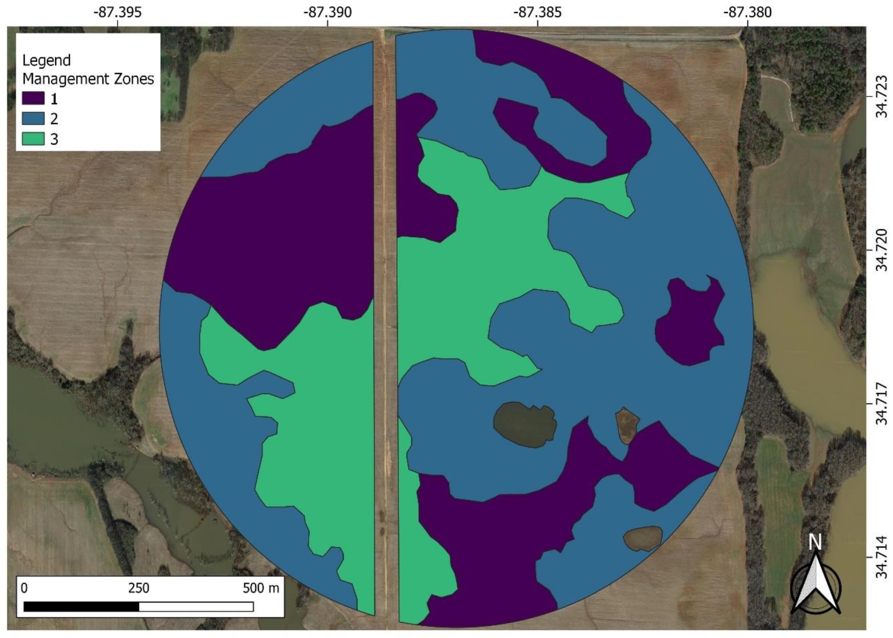
2.1. Study Area

The study was conducted in a commercial cornfield in Lawrence County, Town Creek, Alabama (latitude 34°72′N; longitude 87°39′W), to evaluate the potential of using machine learning models associated with high-resolution satellite data and topographical indices to predict corn yield during the 2018–2019 growing seasons. The predominant soil type in the study field is Decatur silty clay loam with 2–10% slope variation, and the elevation varies between 169 and 180 m. The field was irrigated using a Reinke^© center pivot irrigation system of 623 m length over 125 ha (Figure 1). A description of the sowing, tasseling, and harvest dates for 2018 and 2019 is shown in

Table 2. Description of the operating dates and growth stage of the corn for the years 2018 and 2019.

	Year
	2018	2019
Sowing	10 April	27 March
Tasseling	23 June	9 June
Harvest	3 September	29 August
Corn hybrid	Dekalb® DKC 66-97	Dekalb® DKC 66-97
Row spacing	0.76 m	0.76 m
Plant population	84,000 pl/ha−1	84,000 pl/ha−1

pl/ha⁻¹, plants per hectare.

.

The historic average precipitation for the season (April to August) was 520 mm. The total precipitation was above the historic average for 2018 (640 mm) and 2019 (590 mm). In July 2018 and May, June, and August 2019, the precipitation distribution was below the historic average (Figure 2).

Three MZs were delineated by using information about elevation, slope, and soil texture, and by normalizing yield maps over ten years (Figure 3). This information was used as input into the Management Zone Analyst (MZA) software. This software was used to evaluate the number of homogeneous zones and MZ delineation [43]. We used the unsupervised algorithm fuzzy c-means to divide the field into three cluster classes. After the division, the MZs were adjusted based on known field variability of the farmer and researchers. A description of the soil texture of each MZ is presented in

Table 3. Soil proprieties of the study field.

Management Zone	Soil Type	Sand%	Silt%	Clay%
MZ1 1	Silty clay	13.07	40.13	46.80
MZ2 2	Clay loam	23.20	45.47	31.33
MZ3 3	Clay loam	34.40	31.60	34.00

¹ Management zone one, ² management zone two, ³ management zone three.

. A deeper understanding on how the MZs were delineated can be found in [42].

2.2. Satellite Imagery

The bottom of the atmosphere reflectance Ortho Scene product was acquired from PlanetScope, Planet Labs, Inc., San Francisco, CA, USA [44]. Cloud Planet Scope satellite data provide 3 m spatial resolution images. The data were collected during the critical period for corn yield determination, approximately 20 days before and 20 days after flowering [2,45,46]. One image within this window was chosen for each season (31 May 2019 and 16 June 2018). The PlanetScope satellite data had four spectral bands: blue (455–515 nm), green (500–590 nm), red (590–670 nm), and near-infrared (NIR, 780–860 nm) in a 16-bit GeoTiff format.

We chose the images based on cloud cover and date availability. In the present study, spectral bands with 0% cloud cover over the study area were used to calibrate and validate the models.

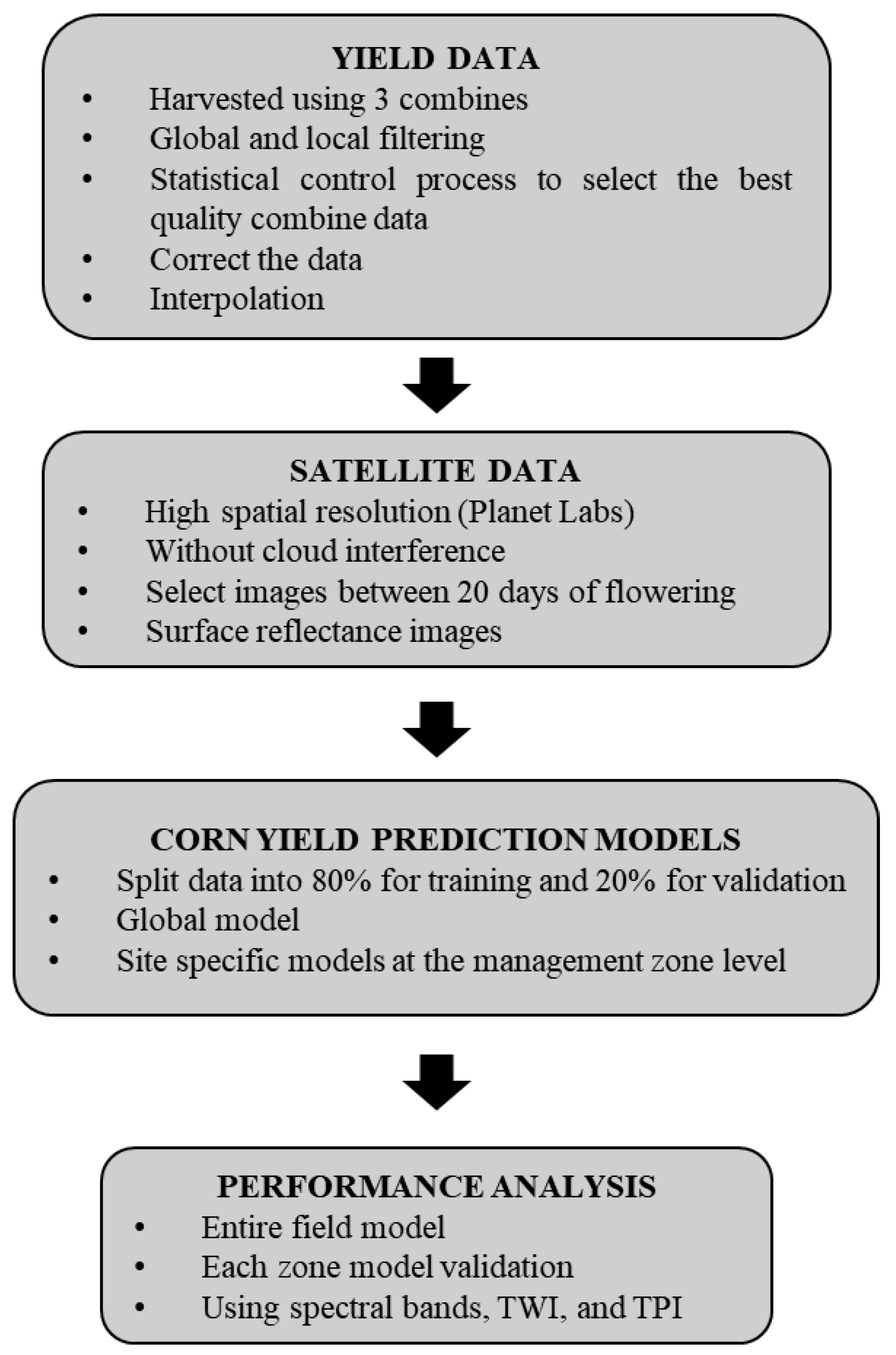
2.3. Data Processing and Building the Dataset

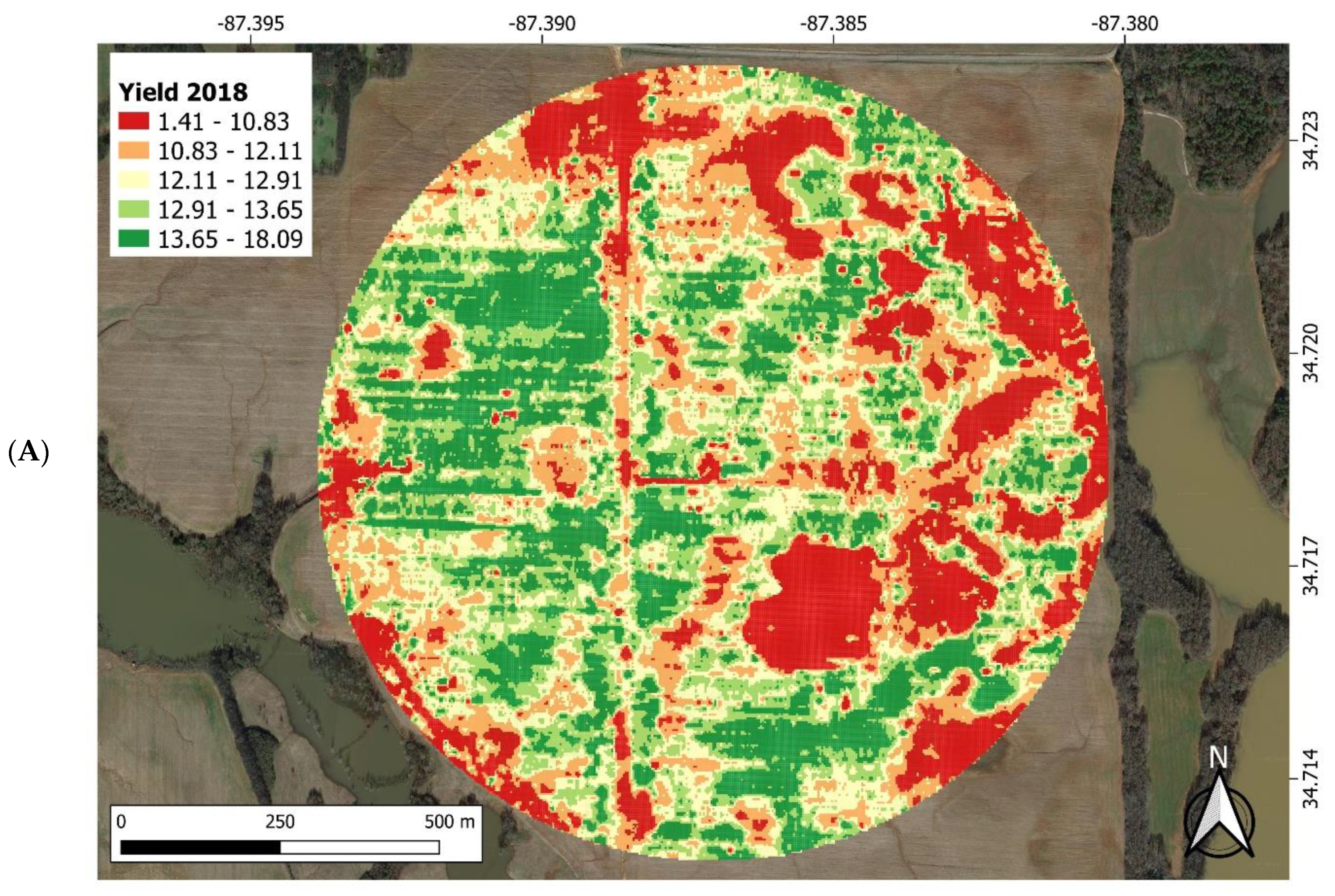
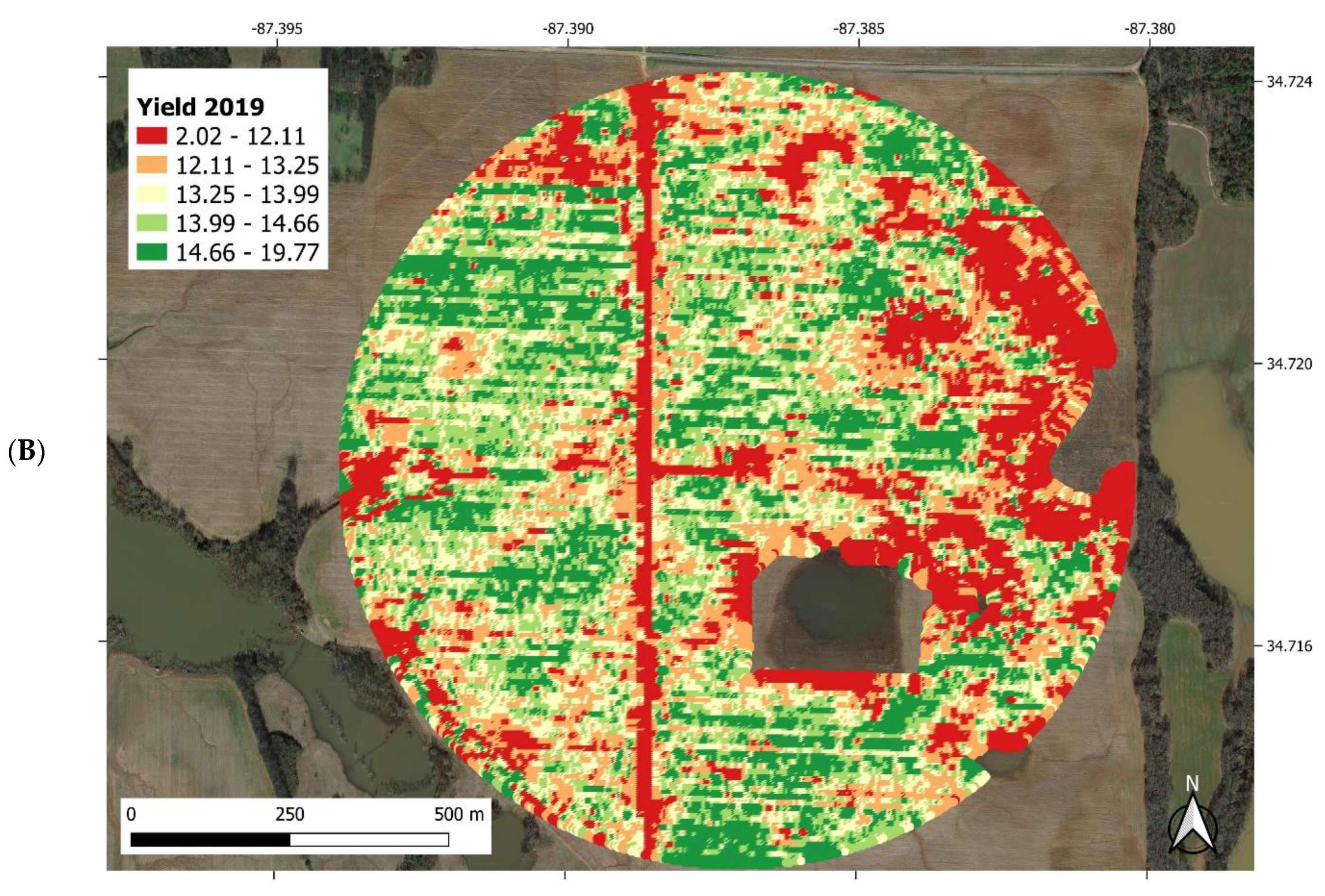
2.3.1. Yield Data

We developed an approach to correct and select quality yield monitor data (from the combine) and satellite data. The yield data were submitted to a filter process to remove global and local outliers. First, yield values equal to 0 were excluded. Second, to remove edge effects and end-of-field yield monitor errors we placed a 30 m buffer distance from the edges (default value). Finally, outlier yield values were those out of the mean ± 3 standard deviation (SD) range. Other filter procedures such as flow and moisture delay, maximum and minimum yield, velocity, and start and end pass delays were performed using Yield Editor. [43] These parameters are specific for each combine and field, so we do not present them in this research. In large fields, farmers generally harvest using more than one combine. In our study area, the field was harvested using three combines (C1, C2, and C3), and we developed a method to correct the data. First, we collected data to represent the spatial variability of the yield and the MZ. All data were collected in parallel passes in which all three combines harvested side by side. To achieve the best quality, we applied statistical control process techniques. This method has been applied previously to evaluate the mechanical harvest process [47,48,49]. The quality of the combines was evaluated using Shewhart’s individual-moving range control charts, in which the central lines correspond to the mean of the calculated values, and the upper and lower control limits (UCL and LCL, respectively) were calculated based on the SDs using the following equations. UCL and LCL are thresholds to determine if a given point is out of the control limits, indicating special causes affecting the analyzed process.

$$UCL=\overline{X}+3\sigma ,$$

(1)

$$\overline{X}=\frac{\left(X1+X2+X3\dots .Xn\right)}{N},$$

(2)

$$LCL=\overline{X}-3\sigma ,$$

(3)

where UCL is the upper control limit, LCL is the lower control limit, $\overline{X}$ is the overall mean, Xn is the value of the sample “n”, N is the total sample number, and σ is the standard deviation. When LCL was negative for I charts, a null value was assigned (LCL = 0).

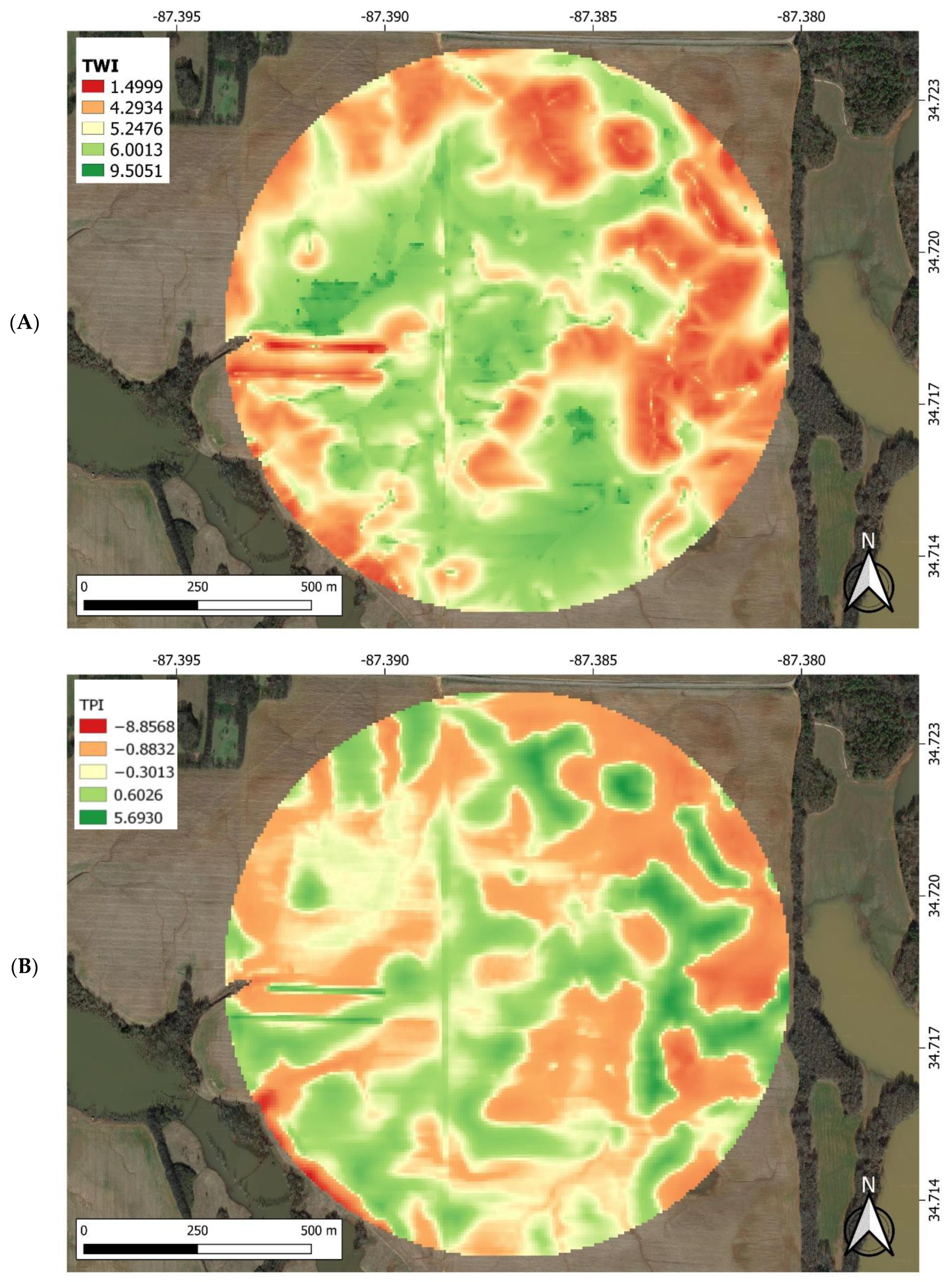
2.3.2. Topographical Data

One of the main pieces of information to generate the TWI is elevation. To obtain this information for the study terrain, a global navigation satellite system with real-time kinematic signal correction was used (John Deere’s Starfire 6000 receiver). This system provides an accuracy close to 2.5 cm on the horizontal coordinates and 5 cm on the vertical coordinates. The data obtained from the global navigation satellite system are geo-object points with X and Y coordinates and elevation. To transform the geo-object points into the geo-field (digital elevation model), we used kriging interpolation for the elevation attribute using ArcMap software (version 10.3.1; ESRI, Redlands, CA, USA).

The TWI and TPI (Figure 4) were calculated using Equations (4) and (5), whereas the catchment area and slope that are required for the TWI equation were obtained using the interpolated map of elevation in the System for Automated Geoscientific Analyses (version 2.3.2):

$$TWI=\ln \left(\frac{A_s}{tan\beta }\right),$$

(4)

$$TPI=z_0-\overline{z },$$

(5)

where A_s is the specific catchment area (m²m⁻¹), β is the slope angle (degrees), z₀ is the central point, and $\overline{z}$ is the average elevation around the central point.

2.3.3. Dataset Extraction and Feature Importance

After correcting the yield data, the data were interpolated using ordinary kriging (Supplementary Material Table S1) to a raster file with the same spatial resolution as the satellite images used (3 m resolution, Figure 5). Then, we collected the centroid of each pixel to build the dataset with the spectral bands, TPI, TWI and interpolated yield. All pixels were labeled with their respective MZ. To minimize the uncertain transitional areas between zones and field border, a buffer of 10 m was applied. All procedures related to this part of the research were performed using the QGIS software.

We used a recursive feature elimination (RFE) method to select features for this study, which is a widely applied method and performed well in previous studies [50,51,52]. It was performed in two steps. First, the estimator was applied to determine the importance of each feature. Then, the feature with the lowest importance score was removed, and the model performance was evaluated. The built-in feature selection method of random forest (RF) was used in this study to derive the importance of each variable in the tree decision [53]. We implemented the process 300 times to obtain the feature importance in step (1) and determined the features to participate in the final modeling in step (2) [54].

2.4. Auto-ML

The open-source auto-ML library H₂O for the Python programming language was used to solve the fundamental problem of deciding which ML algorithm to use in our experiments (H₂O 2020). Extremely randomized trees, gradient boosting machine (GBM), XGBoost algorithms, and stacked ensemble models (SE) were tested with grids of hyperparameters defined by the auto-ML algorithm. For more details regarding each algorithm and how the auto-ML approach works, the library documentation can be accessed [55].

The training phase was performed using 5-fold cross-validation of the data. The dataset was divided into 80% for training and 20% for validation of the models. After removing the 10 m buffer of the area, the dataset points totaled 106,967 for the 2018 season and 91,722 for 2019. The model with the lowest mean absolute error during the validation phase was chosen as the best model for each experiment. A total of 50 models were trained per experiment, and the best model was chosen to show the results.

2.5. Model Performance Analysis

Experiments were developed to define the optimal features of input for the models. We tested the following four approaches: only spectral bands, spectral bands + TPI, spectral bands + TWI, and spectral bands + TPI + TWI. We also explored two approaches for model calibration: 1. the whole-field approach, which involved calibrating and validating a model using data from the entire field, and 2. the MZ model, which involved calibrating and validating a model using data from only one MZ. These experiments were developed in the following three different temporal scenarios: data from the two seasons together (2018 and 2019), only data from 2018, and only data from 2019.

The accuracy and tendency of the proposed models were evaluated by calculating the mean absolute error (MAE) and estimated mean error (EME) according to Equations (6) and (7), respectively.

$$MAE=\frac{{{\displaystyle \sum }}_{i=1}^n(Yes{t}_i-Yob{s}_i)}{n}$$

(6)

$$EME=\frac{{{\displaystyle \sum }}_{i=1}^N\left(Yob{s}_i-\overline{Y}\right)}{N}$$

(7)

where n is the number of data, Yest_i is the value of the variable estimated by the network, Yobs_i is the value of the observed variable, and $\overline{Y}$ is the mean estimated value.

The relative percentage error was calculated to understand the accuracy achieved by the addition of topographic components in the models expressed by the following equation.

$$X=\left|\frac{x1-y}{x1}\right| \ast 100$$

(8)

where X is the relative percentage error, x₁ is the MAE of a model with only spectral bands as features, and y is the MAE of the chosen model.

Performance analyses were performed using a scatter plot of predicted values as the dependent variable (y-axis) and observed values as the independent variable (x-axis), and a line of 1:1 was plotted to determine which model showed values near the line.

2.6. Theoretical Framework

For better understanding of the global approach used to predict the corn yield, a theoretical framework was developed to illustrate the steps developed in this research (Figure 6).

3. Results

The following sections present the results from the approach to predict corn yield at the MZ level using spectral bands and topographical indices. Descriptive statistics were used to characterize the variables during 2018 and 2019. The models were ranked based on the accuracy metric MAE and then the performance of the best models for each experiment was analyzed. The best model from each experiment was used to generate the predicted yield maps to show the spatial variability of the yield.

3.1. Descriptive Statistics of Corn Yield, Spectral Bands, TWI, and TPI

Descriptive statistics of corn yield, spectral bands, and TWI for 2018 and 2019 are shown in

Table 4. Descriptive analysis for spectral bands, TWI, and yield for the years 2018 and 2019.

2018						2019
MZ1
	mean	Std	C.V(%)	min	max		mean	std	C.V(%)	min	max
Blue	5509	72	1	5172	6189	Blue	499	27	5	410	723
Green	4773	58	1	4554	5398	Green	588	32	5	504	819
Red	3238	85	3	2959	4380	Red	557	52	9	443	909
NIR	11,441	290	3	8590	12,435	NIR	3721	159	4	2983	4210
TWI	6	1	20	2	10	TWI	6	1	18	2	10
TPI	−1	1	−158	−5	5	TPI	−1	1	−151	−5	5
Yield	13.25	1.28	9	5.31	17.49	Yield	14.19	1.14	8	2.89	19.77
MZ2
Blue	5576	99	2	5231	6904	Blue	529	35	7	382	702
Green	4857	104	2	4567	5897	Green	626	42	7	473	818
Red	3368	168	5	3031	5101	Red	627	79	13	412	981
NIR	11,126	423	4	5476	12,717	NIR	3686	180	5	1962	4277
TWI	4	1	23	2	9	TWI	4	1	23	2	8
TPI	0	2	413	−9	6	TPI	1	2	309	−9	6
Yield	11.37	1.68	15	3.97	17.75	Yield	13.05	1.68	13	2.35	19.44
MZ3
Blue	5513	79	1	5176	6965	Blue	510	26	5	431	696
Green	4784	68	1	4574	6136	Green	604	31	5	507	808
Red	3255	96	3	3005	5453	Red	579	50	9	453	979
NIR	11,366	273	2	9093	12,499	NIR	3715	121	3	3146	4210
TWI	6	1	15	1	9	TWI	6	1	15	1	9
TPI	0	1	−2218	−3	4	TPI	0	1	−2081	−3	4
Yield	13.05	1.14	9	1.41	17.96	Yield	13.99	1.08	8	3.23	19.17

Spectral bands are expressed in reflectance at a scale factor of 10,000. Yield is expressed in Mg ha. TWI and TPI are dimensionless.

. Comparing the yield between the years and analyzing each MZ, 2019 (14.19 Mg ha⁻¹) showed a higher yield than 2018 (13.25 Mg ha⁻¹). A higher mean yield was observed in MZ1 (13.25 and 14.19 Mg ha⁻¹ for 2018 and 2019, respectively), whereas MZ2 showed the lowest mean yield (11.37 and 13.05 Mg ha⁻¹ for 2018 and 2019, respectively). MZ3 showed the minimum and maximum yield in 2018, whereas in 2019 MZ1 showed maximum yield and MZ2 the minimum. The minimum and maximum yields were found for MZ3 in 2018, whereas in 2019 the maximum yield was observed in MZ1, and the minimum was in MZ2. Therefore, MZ1 was the high-yield zone, MZ2 was the low-yield zone, and MZ3 had an intermediate yield independent of the year analyzed, showing the temporal stability of the MZ. MZ2 was the zone with the highest variability in terms of yield with a mean of 14% of the coefficient of variation (C.V.) when 2018 and 2019 were analyzed.

3.2. Feature Importance

The six features were ranked using the RFE strategy described in Section 2.3.3. The ranking results from the experiment are shown in Supplementary Material Figure S1. Across 300 experiments, the topographic indices have stable ranking order. We can infer that TWI and TPI have higher influence in the models than spectral bands, while the red band showed higher importance among the spectral bands. We can infer from these results that topographic indices show higher importance for ML modeling than spectral reflectance in a field with significant topographic variability.

3.3. Auto-ML for Predicting Corn Yield Using TWI, TPI, and Spectral Bands

For the whole-field models, the stacked ensemble model type showed better accuracy for predicting corn yield in all scenarios, except in 2019, when spectral bands were used as features in the model. This same pattern was also observed for MZ2. For MZ1 and MZ3, GBM was more accurate for predicting corn yield when using spectral bands as features in all scenarios. In contrast, for MZ2 using other features and scenarios, the stacked ensemble model type was more accurate, except when both years were combined and spectral bands + TPI were used as features, in which case the XGBoost model was preferable (

Table 5. Results for training and validation of best models in terms of mean absolute error (MAE, Mg/ha) using data from 2018, 2019, and both years combined.

2018				2019			All Years
Whole Field
	Model Type	Training	Test	Model Type	Training	Test	Model Type	Training	Test
Bands	SE	0.83	0.85	XGBoost	0.78	0.8	SE	0.81	0.84
Bands + TWI	SE	0.4	0.73	SE	0.47	0.73	SE	0.64	0.76
Bands + TPI	SE	0.44	0.75	SE	0.45	0.73	SE	0.63	0.77
Bands + TPI + TWI	SE	0.5	0.65	SE	0.42	0.66	SE	0.57	0.68
MZ1
Bands	GBM	0.73	0.76	GBM	0.67	0.69	GBM	0.7	0.74
Bands + TWI	SE	0.49	0.64	SE	0.39	0.62	SE	0.36	0.63
Bands + TPI	SE	0.19	0.62	SE	0.3	0.62	XGBoost	0.36	0.63
Bands + TPI + TWI	SE	0.1	0.47	SE	0.16	0.52	SE	0.19	0.5
MZ2
Bands	SE	0.83	0.88	XGBoost	0.91	0.97	SE	0.85	0.92
Bands + TWI	SE	0.38	0.75	SE	0.44	0.85	SE	0.45	0.79
Bands + TPI	SE	0.4	0.74	SE	0.41	0.85	SE	0.46	0.78
Bands + TPI + TWI	SE	0.15	0.59	SE	0.22	0.72	SE	0.45	0.68
MZ3
Bands	GBM	0.72	0.73	GBM	0.63	0.64	GBM	0.67	0.68
Bands + TWI	XGBoost	0.38	0.64	XGBoost	0.32	0.59	XGBoost	0.31	0.61
Bands + TPI	SE	0.25	0.62	XGBoost	0.33	0.59	XGBoost	0.32	0.6
Bands + TPI + TWI	SE	0.11	0.48	XGBoost	0.25	0.51	SE	0.19	0.49

SE: stacked ensemble model; GBM: gradient boost machine; TWI: topographic wetness index; TPI: topographic position index; MZ1, MZ2, and MZ3: high, low, and intermediate yield zones, respectively.

).

The stacked ensemble models showed better accuracy for predicting corn yield independently of the approach of a general model for all areas and specific models for each MZ when spectral bands + TWI were used as features (Table 5). Using only spectral bands as features in the models, for MZ1, the GBM algorithm showed better accuracy, whereas for MZ2, MZ3, and all areas, the stacked ensemble algorithm showed better accuracy (Table 5). Higher accuracy was achieved using spectral bands + TWI as features, and the highest accuracy was for the stacked ensemble model in MZ1.

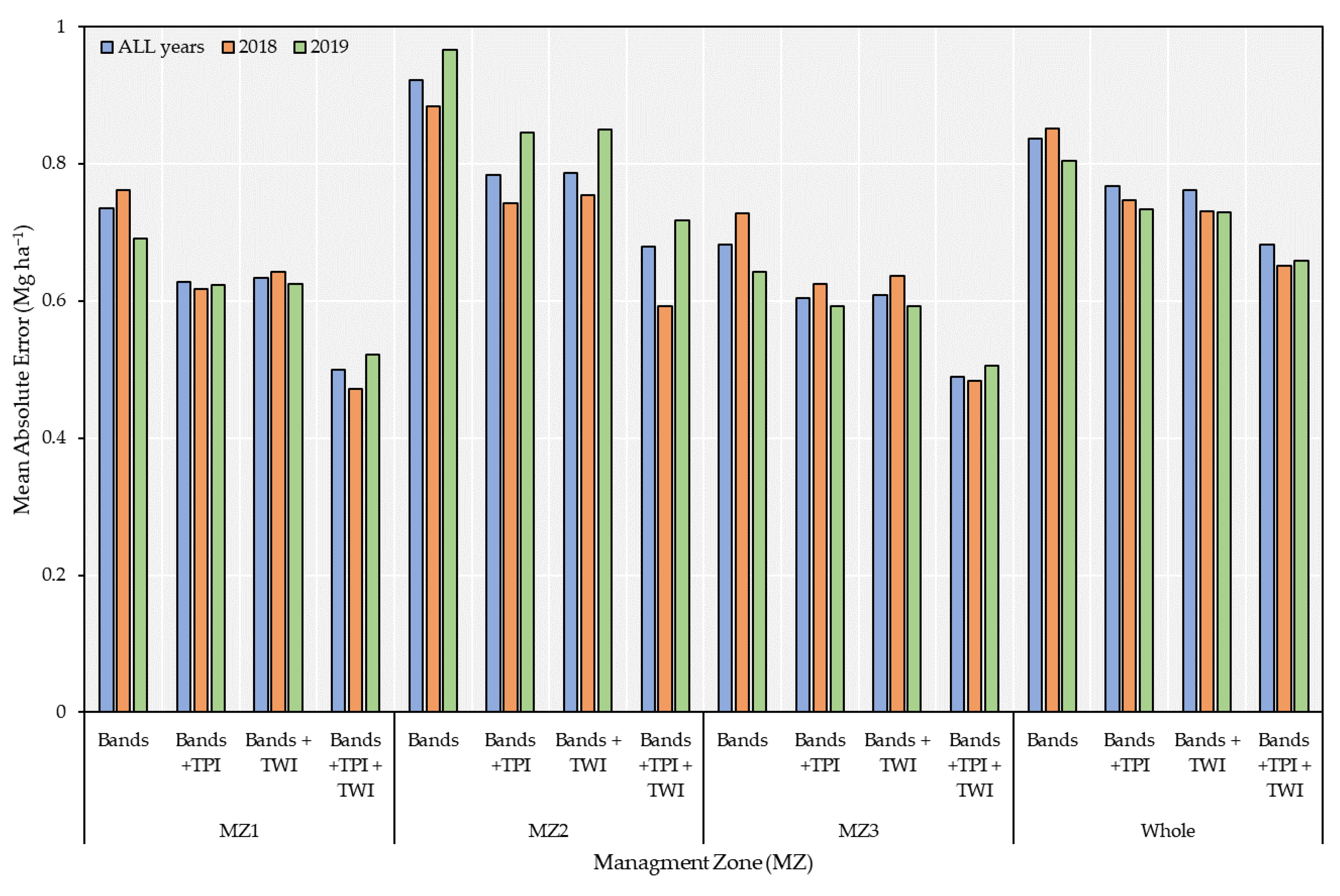
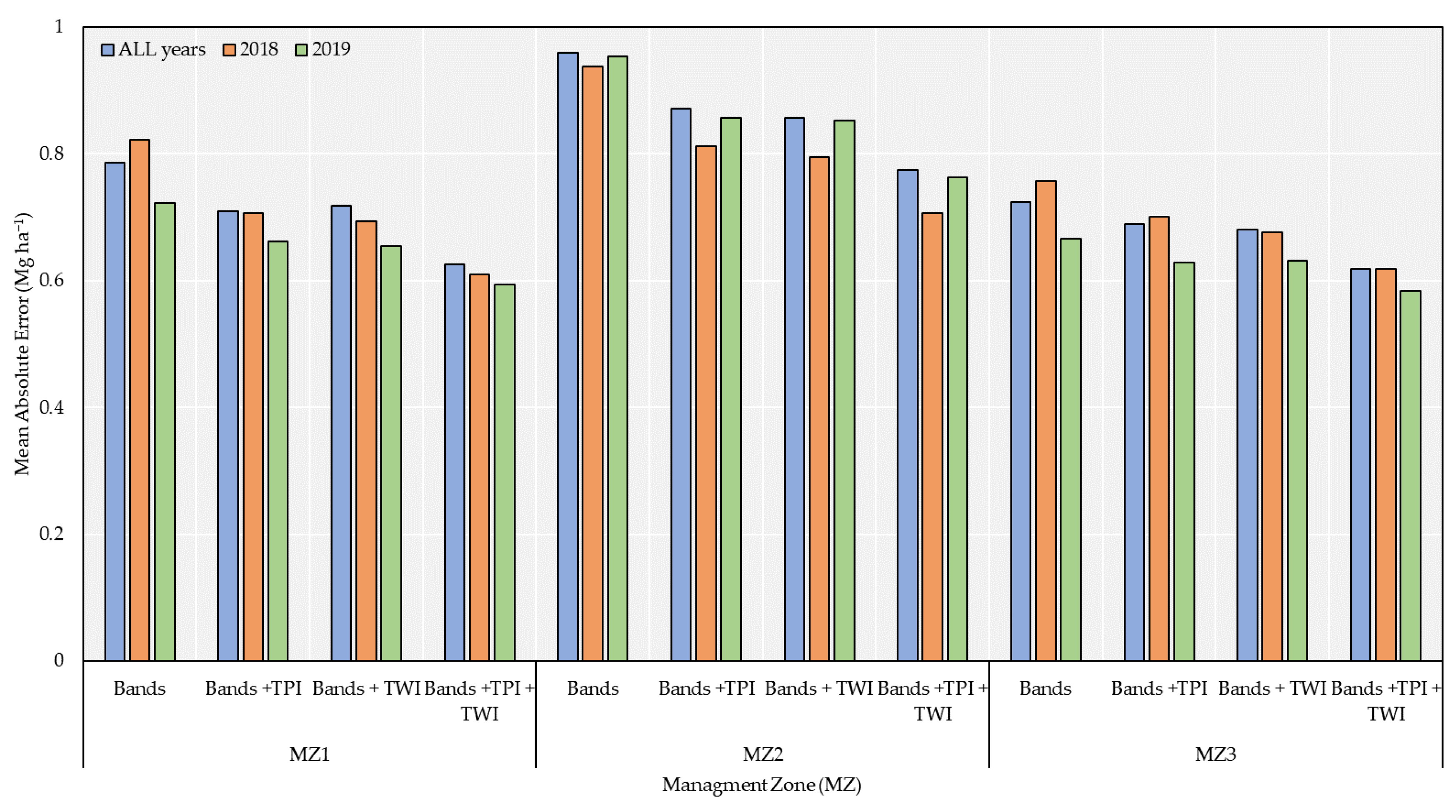
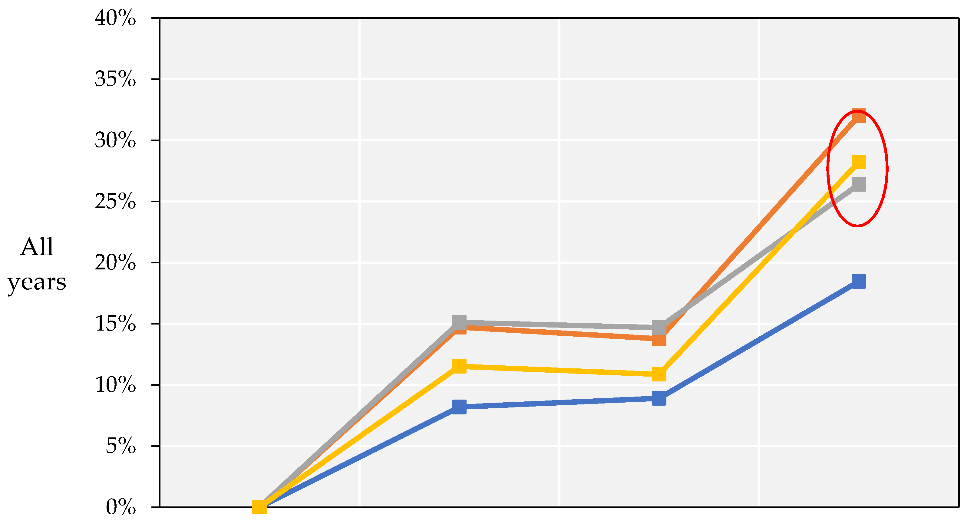
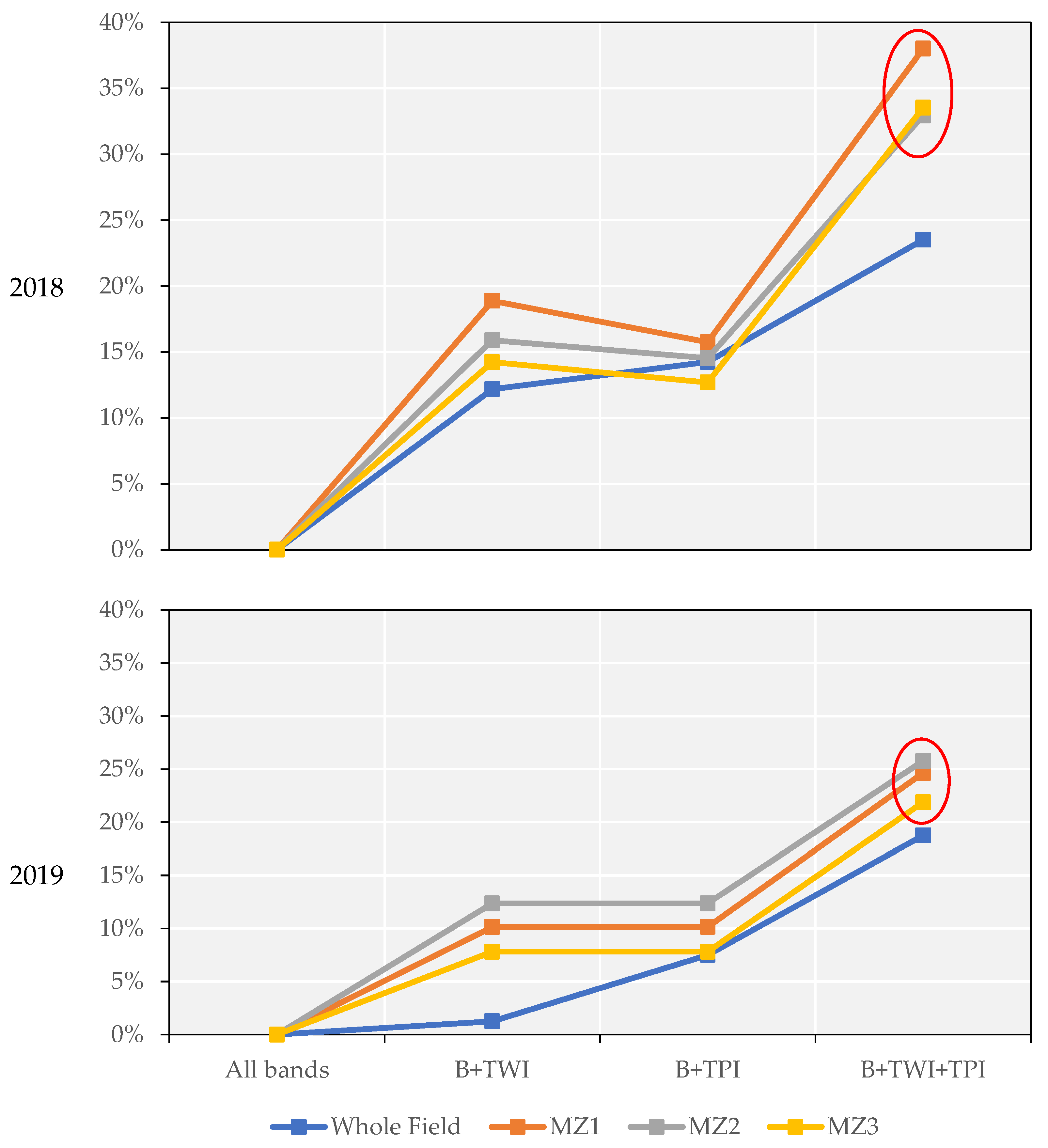
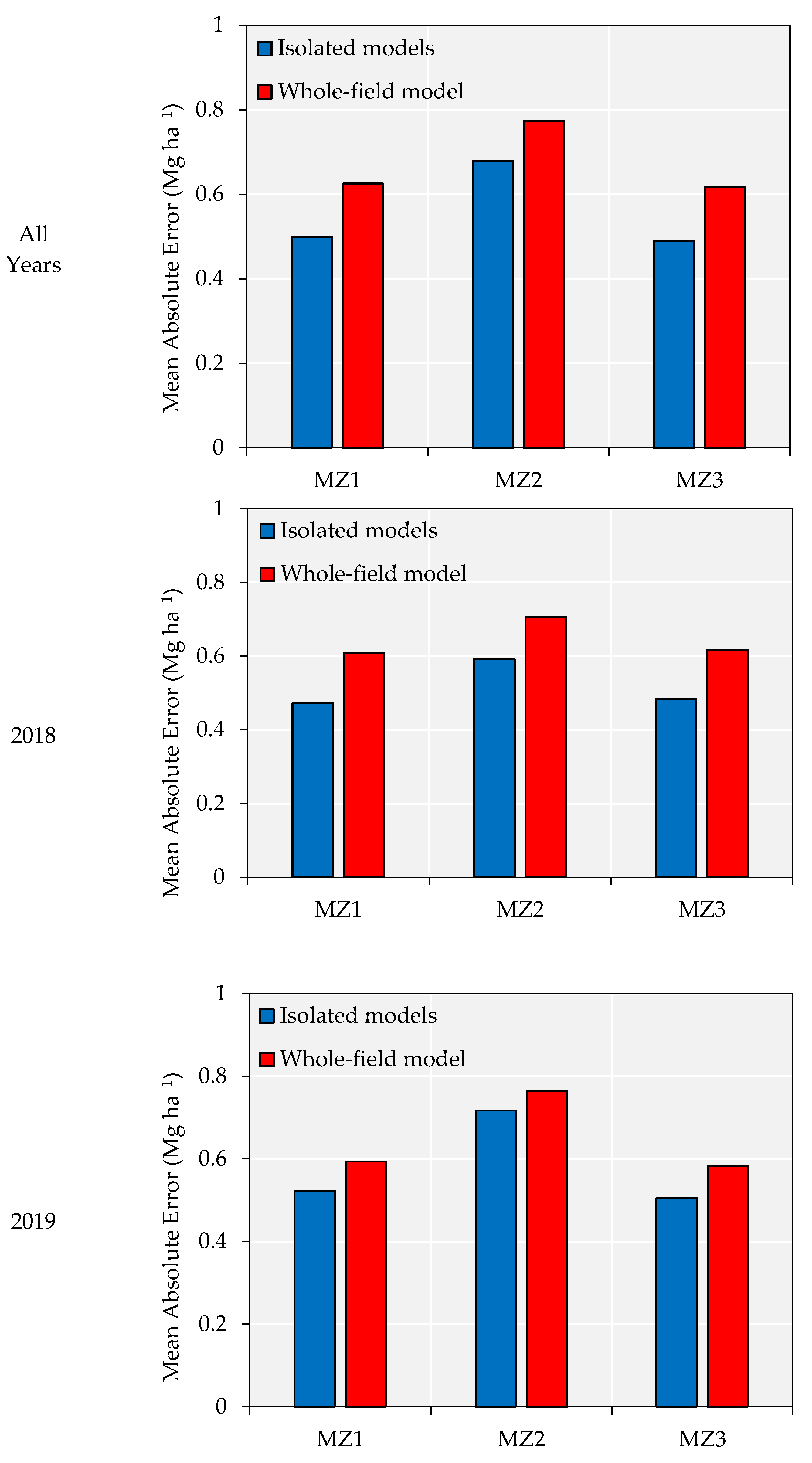
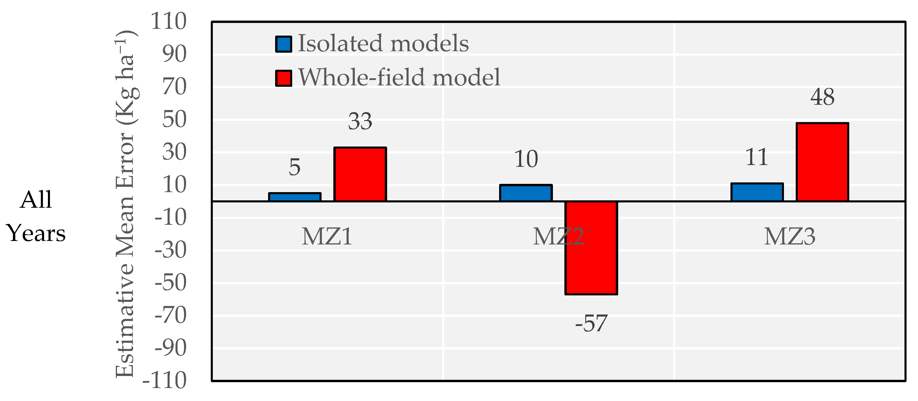
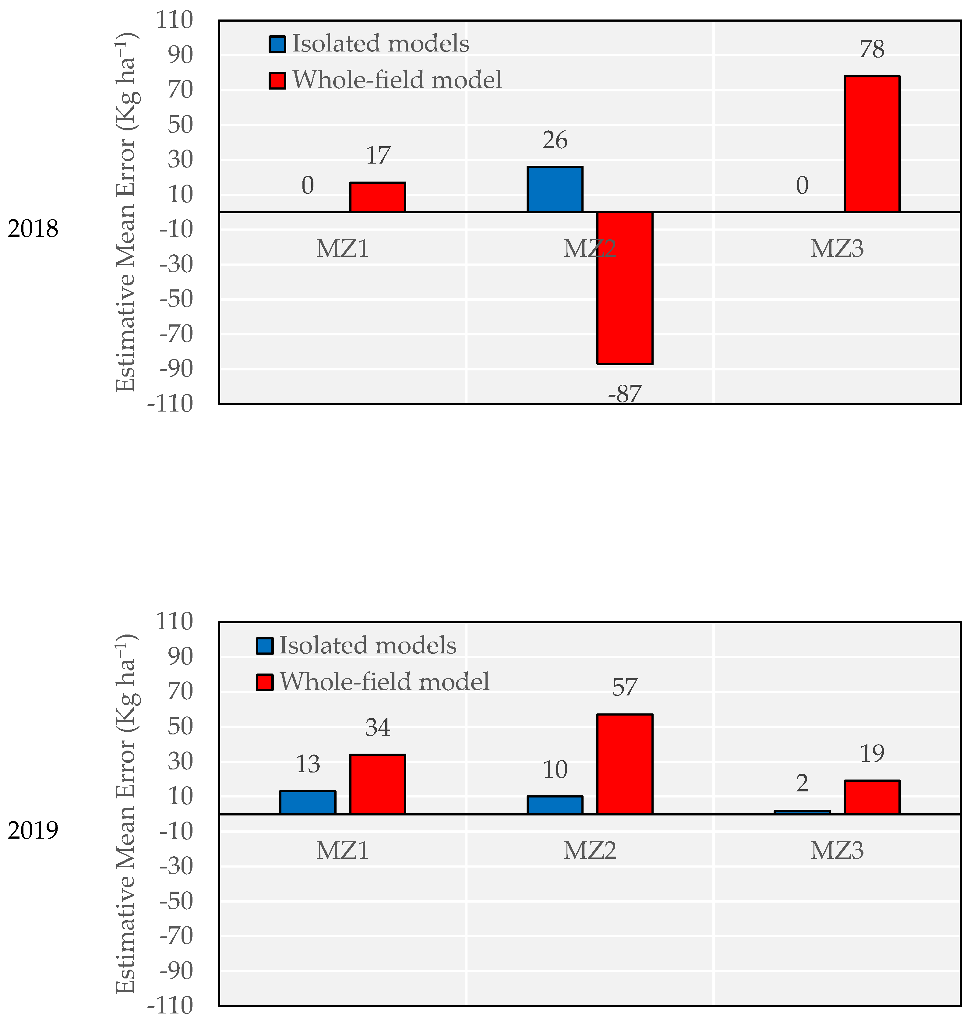
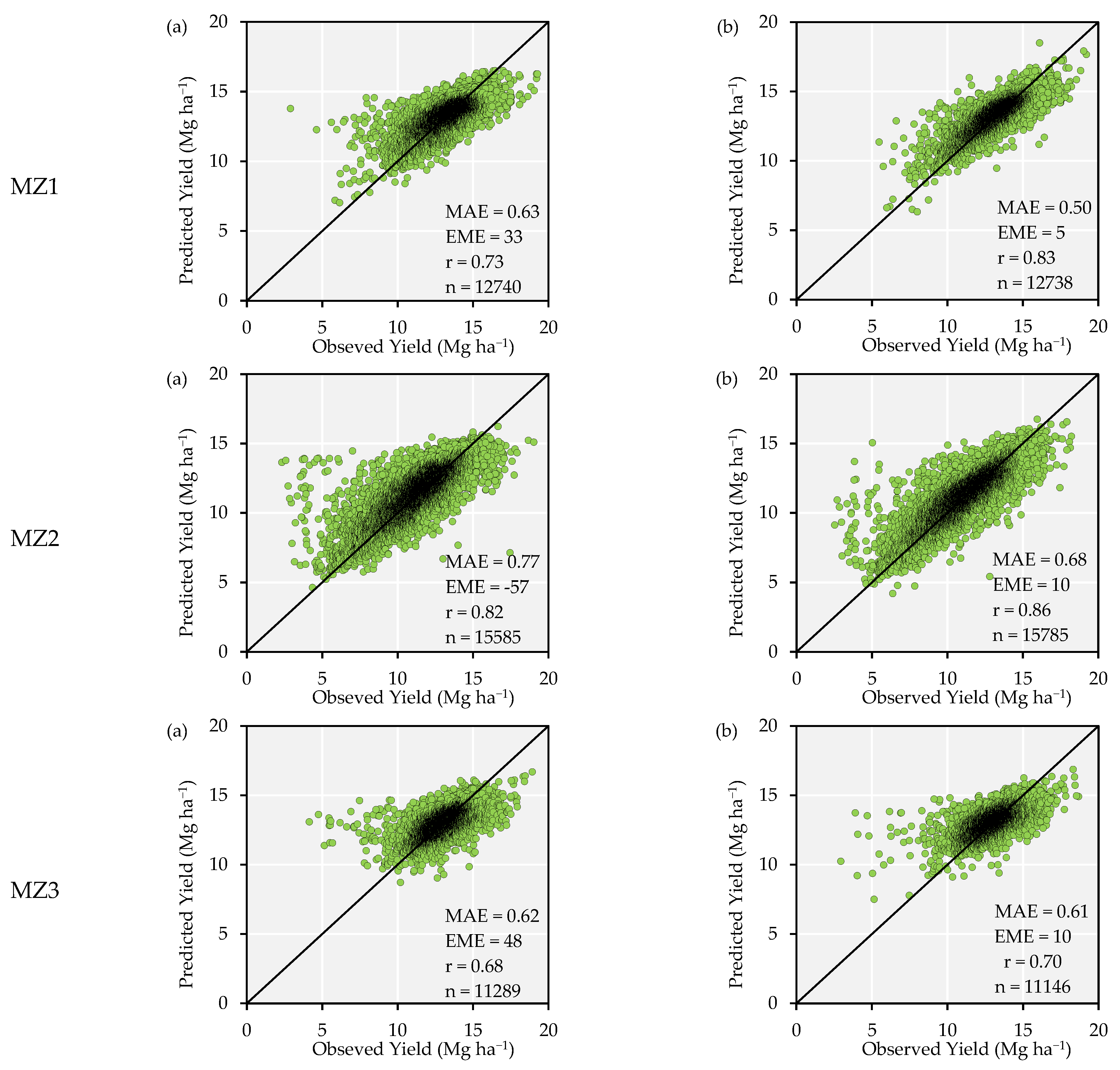
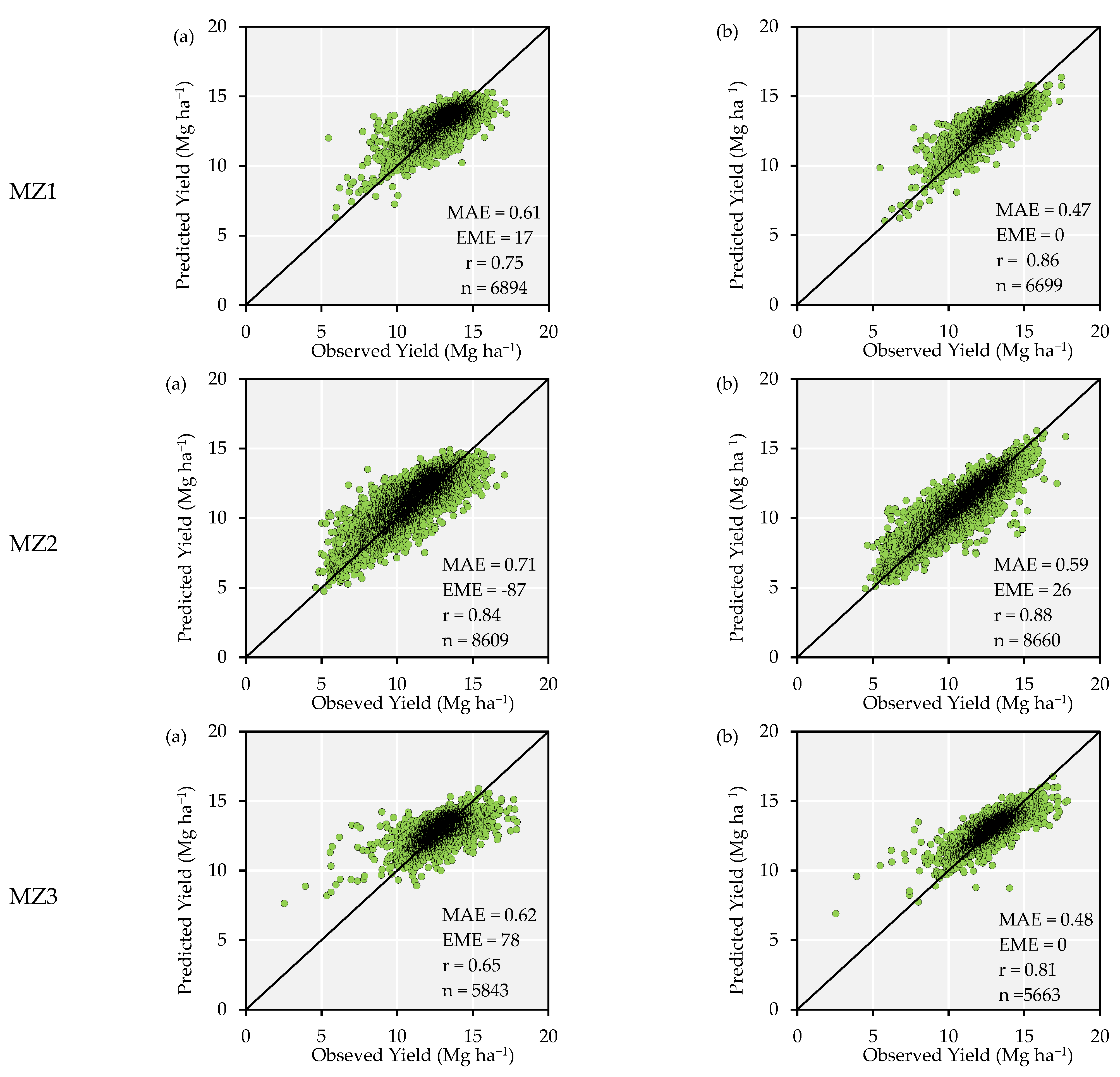
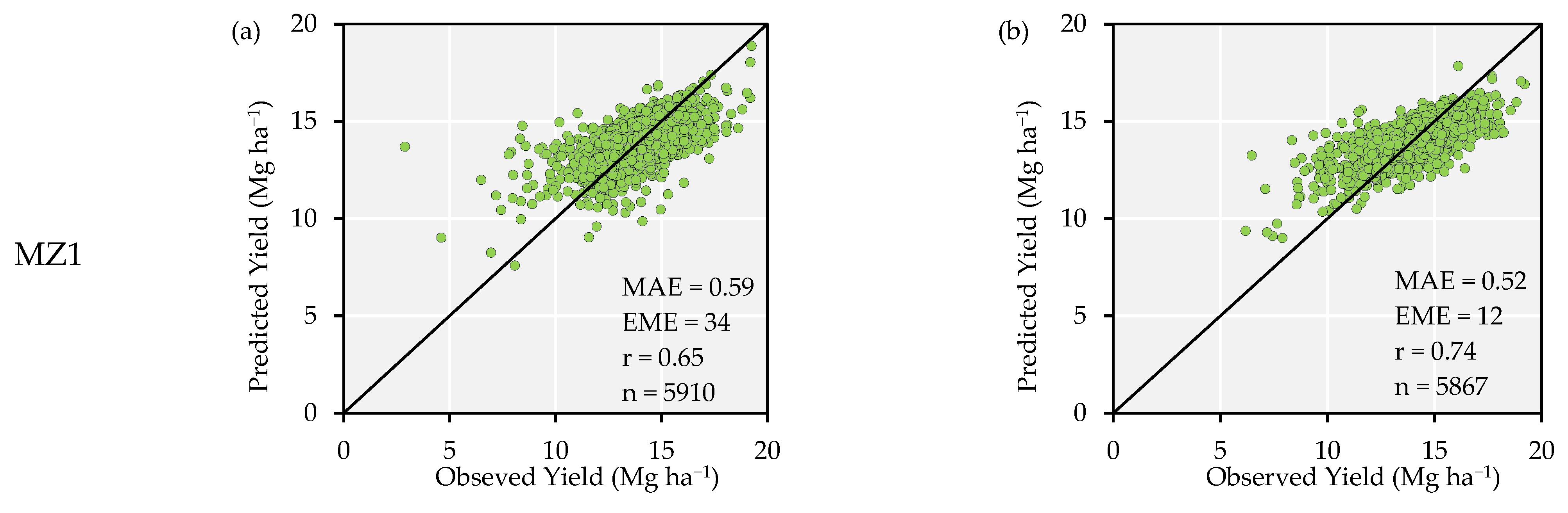
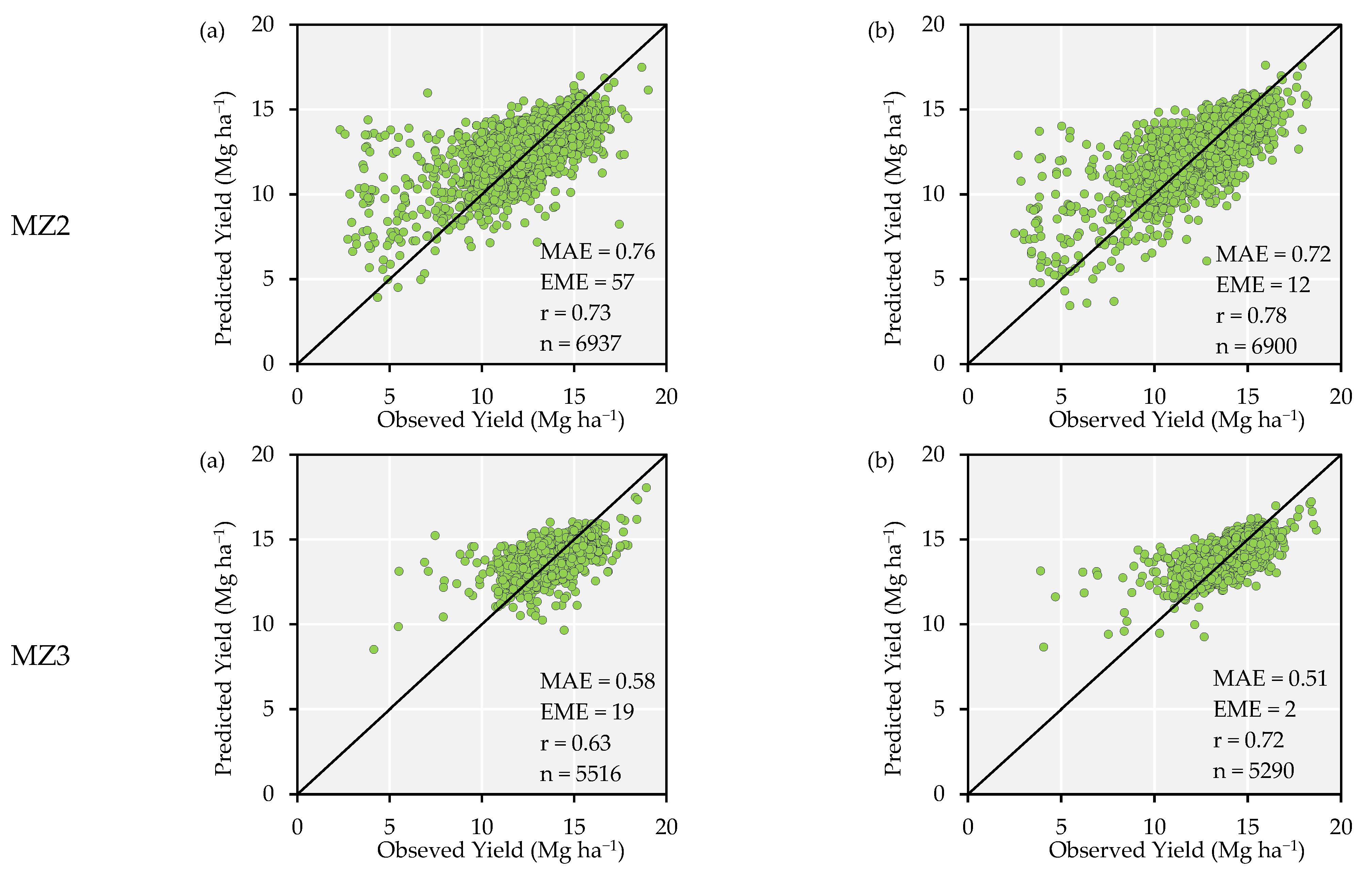
3.4. Comparison of Models Using Different Features in Three Scenarios in Terms of Accuracy, Relative Error, and Tendency

Figure 7 shows the results of the accuracy metric (MAE) as reported in Equation (6). The MAE can distinguish which feature combination was the most accurate for predicting corn yield. Based on this metric, the models had the lowest accuracy (highest MAE) when only the spectral bands were used, whereas when the models used spectral bands, TWI, and TPI as features, the highest accuracy (lowest MAE) for predicting the corn yield for all scenarios (all years combined and 2018 and 2019 seasons) was obtained. When the models used TWI or TPI as features, the accuracy was similar in all scenarios. The whole-field model showed lower accuracy for the feature combinations of spectral bands + TPI, spectral bands + TWI, and spectral bands + TPI + TWI in all scenarios analyzed as compared to the MZ1 and MZ3 site-specific models. The MZ2 site-specific model showed a similar accuracy to that of the whole-field model.

The specific accuracy of the whole-field model was lower in MZ2 compared to MZ1 and MZ3. These models had difficulty predicting corn yield in low-yield zones (Figure 8). The spectral bands + TPI + TWI features had a higher accuracy than those of the other combination of features.

To determine whether the association between topographical indices and spectral bands could increase the accuracy of the yield forecasting, we calculated the relative error of the models when only spectral bands were used as features (Figure 9). Analyzing all scenarios, isolated seasons (2018 and 2019), and combined seasons, including spectral bands + TWI + TPI as features, the models obtained a better accuracy, whereas accuracy was higher for site-specific models (Figure 8). For the scenario of the isolated season and site-specific models, the models using spectral bands + TWI and spectral bands + TPI showed a similar increase in accuracy to that of the models using only spectral bands.

To compare the accuracy of the whole-field model and isolated model, we analyzed the specific accuracy of the best feature combination (spectral bands + TPI + TWI) against the accuracy of the specific models for each MZ (high, low, and intermediate yields; Figure 10) for the two scenarios (all years combined and specific season, 2018 and 2019). For all scenarios analyzed, the specific models showed better accuracy (lower MAE) than the whole-field model; however, for better understanding, and not only accuracy, it is enough to decide if we need site-specific models or a whole-field model.

To analyze the tendency of the models, the EME was calculated and compared in the three scenarios (all years combined, 2018, and 2019) using models with spectral bands + TWI + TPI as features. All the comparisons were performed using specific models compared to the whole-field model, using its tendency in each MZ. The tendency metric allowed us to understand whether the model was underestimating or overestimating the yield prediction and to infer which approach had a lower tendency and which MZ occurred. For all years, the whole-field model underestimated the corn yield (−57 kg ha⁻¹) in MZ2 (low-yield zone). Whereas for MZ1 (33 kg ha⁻¹) and MZ3 (48 kg ha⁻¹) the model overestimated. The MZ1 model (high-yield zone) showed approximately 55% lower tendency than the whole-field model in MZ1. This value had approximately 77% lower tendency for the model trained and validated using only the MZ3 data compared to the whole-field model (Figure 11). Underestimation of MZ2 was observed in the 2018 scenario (−87 kg ha⁻¹), whereas in 2019 the whole-field model showed an overestimation (57 kg ha⁻¹). The lowest tendency was observed in 2018 using site-specific models for MZ1 and MZ3, which was approximately zero. Based on these results, using site-specific models had lower tendency than using the whole-field model.

To analyze the performance of the chosen models, the corn yield forecasted by the resultant model during the validation phase was compared with the observed yield (Figure 12, Figure 13 and Figure 14). The results for the models using combined data and the separate growing seasons (2018 and 2019) suggested that it was possible to forecast corn yield with reasonable accuracy using data combining spectral bands + TPI + TWI as features. A general behavior independent of using data from a specific MZ or the entire field was that the accuracy of the models was lower when predicting the yield in a low-yield area (MZ2). Building a model with data from a high-yield zone (MZ1) and using spectral bands, TPI, and TWI as features was the most accurate for forecasting corn yield (MAE = 0.47).

Our second observation supports the hypothesis that site-specific models using spectral bands, TPI, and TWI as features had different accuracies depending on the MZ used for the calibration and validation (MAE MZ1 = 0.50, MAE MZ2 = 0.68, and MAE MZ3 = 0.49). This leads us to infer that for MZs representing low-yield zones (MZ2), the corn yield forecasting accuracy was compromised due to lower accuracy (higher MAE and EME) (Figure 12).

4. Discussion

In the present study, a method for developing site-specific models for corn yield modeling at the MZ level was proposed, and the results showed that it is possible to predict corn yield with reasonable accuracy using spectral crop information associated with TWI and TPI during the flowering growth stage. Therefore, the association of spectral and topographical data can increase the accuracy of crop yield prediction. We demonstrated that machine learning could predict the yield pattern at the management zones. We highlight that to use this framework, it is important to develop management zones to calibrate MZ models that use spectral bands and topographic indices. We do not recommend the cross use of these models, because we developed models using specific yield variability. Models should be developed and used for the management zone where they were trained.

The first and most important outcome from the present study was the possibility to predict corn yield using only spectral bands. However, to obtain a more accurate model, spectral bands with TPI and TWI, which are surface-related variables, should be used (Figure 7). The importance of surface structure (slope) variables on crop yield prediction has been shown by [56]. Surface variables explain yield variability components such as the spatial patterns of soil, water, and nutrient distribution [57]. The increase in accuracy from adding the topographical indices (spectral bands + TPI + TWI as features, Figure 9) can be explained by the addition of deterministic variables (equations of the topographical indices), which are consistent throughout time. These topographical indices have been generated from elevation data derived from yield monitoring, and field elevation remains the same unless the farmer modifies the field surface, which is not common. Another factor that can increase accuracy is topography’s influence on hydrological processes [7]. These processes are related to the spatial distribution of groundwater flow and soil moisture [8]. Soil moisture is correlated with TWI [58], reflecting the water availability for crop growth and development [59], and can ultimately affect yield. The TPI is a topography-derived index that considers the local topography for a given region [60] and is also correlated with yield [61]. The authors of [56] highlighted the necessity of exploring the inclusion of microtopography metrics derived from slope data to predict within-field variability accurately during a growing season, and our approach could be a promising application in this field.

The second result from our analysis showed the potential for the development of site-specific models at the MZ level due to a lower tendency (Figure 9) and higher accuracy (Figure 10). Site-specific crop management in terms of resource use efficiency can be enhanced by identifying homogenous MZs [62]. Crop management is changing from large-scale operations to precision agriculture, which requires technologies to forecast yield by considering within-field variation [2]. Our approach to modeling corn yield could aid with precision agricultural technologies. These models could predict within-field yield variability, which can be used to characterize the factors (environmental conditions and management practices) that contribute to yield variability. The models are also suitable for capturing critical site-specific factors that drive inter-region or in-field variability. Our results, in terms of modeling crop yield at the field level, agree with several previous studies [2,3,35,56] that have successfully developed models to forecast yield at field level. To the best of our knowledge, no other study has attempted to forecast corn yield associated with TWI, TPI, spectral bands, and ML algorithms. There is a demand for crop modeling tools that involve multiple sources of data to improve the prediction accuracy of the crop yield.

From a practical standpoint, farmers, who have yield monitors, already collect high-quality data during harvest (i.e., yield and elevation); therefore, these available data can be used to derive TWI and TPI microtopography that, along with high-resolution remote sensing imagery collected at the time of flowering, can be used for corn yield prediction prior to harvest. This prediction might allow farmers to determine the spatial within-field variability of the yield before harvesting and make either adjustments in management or adjust the corn market price. The predictive yield maps at the MZ level would be valuable for farmers when planning their MZ land use to achieve their production goals and determine the harvester settings. Farmers might also use a higher-quality combine to harvest a high-yield zone. Upscaling this method for larger areas can help the research community to understand yield variability and the impact of irrigation use and climate. Areas of higher risk can be identified, and farmers can mitigate yield losses through the purchase of crop insurance or by leaving some areas of a field out of production. To scale up the proposed yield prediction method, some processes should be implemented, for example, algorithmic automation of TPI and TWI generation and management zone delineation. Transfer learning theory could be applied to improve this method. We could use country- or county-level models and incorporate the information at the management zone level for better predictability, since time series of yield monitor data are common in farms, but these data are not fully used to build prediction models.

Scaling up the proposed methodology to many regions of the southeast could have positive socioeconomic and environmental consequences. Corn yield predictions could be useful in understanding the impact of irrigation and nitrogen management, which could be useful to support adoption of site-specific irrigation and nitrogen management practices. Depending on the patterns of corn yield variability, increased access to conservation programs might be available to farmers, as well as crop insurance. Farmers, overall, could receive more support from governmental agencies, extension services, and private industry.

5. Conclusions

The present study investigated the potential of using spectral bands of high-resolution satellite images and topographical indices to create site-specific models using auto-ML algorithms. Knowing that topographical indices can explain site-specific yield variability is important for crop yield modeling and for supporting management decisions based on yield forecasting. As studies within yield forecasting have focused on large-scale approaches, the present study provides evidence that contributes to crop yield modeling at the MZ level.

Topographical indices increase the accuracy of corn yield forecasting when associated with spectral bands as features of ML models.

Site-specific models are required to increase the accuracy and reduce the tendency of corn yield forecasting on MZs with high, low, and intermediate yields. The most important features for modeling corn yield were spectral bands + TPI + TWI.

Auto-ML using the stacked ensemble algorithm can be used to forecast corn yield before harvesting by using combined data from different seasons.

Future studies should focus on testing this method using fields with different topographical characteristics to understand if the topography indices have the same behavior in the models developed in high and low slope areas.

References

1. Venancio, L.P.; Mantovani, E.C.; do Amaral, C.H.; Usher Neale, C.M.; Gonçalves, I.Z.; Filgueiras, R.; Campos, I. Forecasting corn yield at the farm level in Brazil based on the FAO-66 approach and soil-adjusted vegetation index (SAVI). Agric. Water Manag. 2019, 225, 105779. [Google Scholar] [CrossRef]
2. Peralta, N.; Assefa, Y.; Du, J.; Barden, C.; Ciampitti, I. Mid-Season High-Resolution Satellite Imagery for Forecasting Site-Specific Corn Yield. Remote Sens. 2016, 8, 848. [Google Scholar] [CrossRef] [Green Version]
3. Kayad, A.; Sozzi, M.; Gatto, S.; Marinello, F.; Pirotti, F. Monitoring Within-Field Variability of Corn Yield using Sentinel-2 and Machine Learning Techniques. Remote Sens. 2019, 11, 2873. [Google Scholar] [CrossRef] [Green Version]
4. Al-Gaadi, K.A.; Hassaballa, A.A.; Tola, E.K.; Kayad, A.G.; Madugundu, R.; Assiri, F.; Alblewi, B. Characterization of the spatial variability of surface topography and moisture content and its influence on potato crop yield. Int. J. Remote Sens. 2018, 39, 8572–8590. [Google Scholar] [CrossRef]
5. Yu, B.; Shang, S. Multi-year mapping of major crop yields in an irrigation district from high spatial and temporal resolution vegetation index. Sensors 2018, 18, 3787. [Google Scholar] [CrossRef] [Green Version]
6. Chlingaryan, A.; Sukkarieh, S.; Whelan, B. Machine learning approaches for crop yield prediction and nitrogen status estimation in precision agriculture: A review. Comput. Electron. Agric. 2018, 151, 61–69. [Google Scholar] [CrossRef]
7. Sørensen, R.; Zinko, U.; Seibert, J. On the calculation of the topographic wetness index: Evaluation of different methods based on field observations. Hydrol. Earth Syst. Sci. 2006, 10, 101–112. [Google Scholar] [CrossRef] [Green Version]
8. Zinko, U.; Seibert, J.; Dynesius, M.; Nilsson, C. Plant species numbers predicted by a topography-based groundwater flow index. Ecosystems 2005, 8, 430–441. [Google Scholar] [CrossRef]
9. McCann, B.L.; Pennock, D.J.; van Kessel, C.; Walley, F.L. The Development of Management Units for Site-Specific Farming. In Proceedings of the Third International Conference on Precision Agriculture, Minneapolis, MN, USA, 23–26 June 1996; Robert, P.C., Rust, R.H., Larson, W.E., Eds.; American Society of Agronomy: Madison, WI, USA; Crop Science Society of America: Fitchburg, WI, USA; Soil Science Society of America: Madison, WI, USA, 1996; pp. 295–302. [Google Scholar]
10. Kaspar, T.C.; Colvin, T.S.; Jaynes, D.B.; Karlen, D.L.; James, D.E.; Meek, D.W.; Pulido, D.; Butler, H. Relationship between six years of corn yields and terrain attributes. Precis. Agric. 2003, 4, 87–101. [Google Scholar] [CrossRef]
11. Moore, I.D.; Grayson, R.B.; Ladson, A.R. Digital terrain modelling: A review of hydrological, geomorphological, and biological applications. Hydrol. Process. 1991, 5, 3–30. [Google Scholar] [CrossRef]
12. Burt, T.; Butcher, D. Stimulation from simulation? A teaching model of hillslope hydrology for use on microcomputers. J. Geogr. High. Educ. 1986, 10, 23–39. [Google Scholar] [CrossRef]
13. Moore, I.D.; Gessler, P.E.; Nielsen, G.A.; Peterson, G.A. Soil Attribute Prediction Using Terrain Analysis. Soil Sci. Soc. Am. J. 1993, 57. [Google Scholar] [CrossRef]
14. Qin, C.-Z.; Zhu, A.-X.; Pei, T.; Li, B.-L.; Scholten, T.; Behrens, T.; Zhou, C.-H. An approach to computing topographic wetness index based on maximum downslope gradient. Precis. Agric. 2011, 12, 32–43. [Google Scholar] [CrossRef]
15. Silva, J.R.M.D.; Alexandre, C. Spatial Variability of Irrigated Corn Yield in Relation to Field Topography and Soil Chemical Characteristics. Precis. Agric. 2005, 6, 453–466. [Google Scholar] [CrossRef]
16. Maestrini, B.; Basso, B. Drivers of within-field spatial and temporal variability of crop yield across the US Midwest. Sci. Rep. 2018, 8, 1–9. [Google Scholar] [CrossRef] [Green Version]
17. Reu, J.D.; Bourgeois, J.; Bats, M.; Zwertvaegher, A.; Gelorini, V.; Smedt, P.D.; Chu, W.; Antrop, M.; Maeyer, P.D.; Finke, P.; et al. Geomorphology Application of the topographic position index to heterogeneous landscapes. Geomorphology 2013, 186, 39–49. [Google Scholar] [CrossRef]
18. Foster, T.; Gonçalves, I.Z.; Campos, I.; Neale, C.M.U.; Brozović, N. Assessing landscape scale heterogeneity in irrigation water use with remote sensing and in situ monitoring. Environ. Res. Lett. 2019, 14, 024004. [Google Scholar] [CrossRef]
19. Battude, M.; Al Bitar, A.; Morin, D.; Cros, J.; Huc, M.; Marais Sicre, C.; Le Dantec, V.; Demarez, V. Estimating maize biomass and yield over large areas using high spatial and temporal resolution Sentinel-2 like remote sensing data. Remote Sens. Environ. 2016, 184, 668–681. [Google Scholar] [CrossRef]
20. Veloso, A.; Mermoz, S.; Bouvet, A.; Le Toan, T.; Planells, M.; Dejoux, J.F.; Ceschia, E. Understanding the temporal behavior of crops using Sentinel-1 and Sentinel-2-like data for agricultural applications. Remote Sens. Environ. 2017, 199, 415–426. [Google Scholar] [CrossRef]
21. Liu, J.; Pattey, E.; Miller, J.R.; McNairn, H.; Smith, A.; Hu, B. Estimating crop stresses, aboveground dry biomass and yield of corn using multi-temporal optical data combined with a radiation use efficiency model. Remote Sens. Environ. 2010, 114, 1167–1177. [Google Scholar] [CrossRef]
22. Jin, X.; Kumar, L.; Li, Z.; Feng, H.; Xu, X.; Yang, G.; Wang, J. A review of data assimilation of remote sensing and crop models. Eur. J. Agron. 2018, 92, 141–152. [Google Scholar] [CrossRef]
23. Xie, Y.; Wang, P.; Bai, X.; Khan, J.; Zhang, S.; Li, L.; Wang, L. Assimilation of the leaf area index and vegetation temperature condition index for winter wheat yield estimation using Landsat imagery and the CERES-Wheat model. Agric. For. Meteorol. 2017, 246, 194–206. [Google Scholar] [CrossRef]
24. Lopresti, M.F.; Di Bella, C.M.; Degioanni, A.J. Relationship between MODIS-NDVI data and wheat yield: A case study in Northern Buenos Aires province, Argentina. Inf. Process. Agric. 2015, 2, 73–84. [Google Scholar] [CrossRef] [Green Version]
25. Lobell, D.B. The use of satellite data for crop yield gap analysis. F. Crop. Res. 2013, 143, 56–64. [Google Scholar] [CrossRef] [Green Version]
26. Řezník, T.; Pavelka, T.; Herman, L.; Lukas, V.; Širůček, P.; Leitgeb, Š.; Leitner, F. Prediction of Yield Productivity Zones from Landsat 8 and Sentinel-2A/B and Their Evaluation Using Farm Machinery Measurements. Remote Sens. 2020, 12, 1917. [Google Scholar] [CrossRef]
27. Zhao, Y.; Potgieter, A.B.; Zhang, M.; Wu, B.; Hammer, G.L. Predicting Wheat Yield at the Field Scale by Combining High-Resolution Sentinel-2 Satellite Imagery and Crop Modelling. Remote Sens. 2020, 12, 1024. [Google Scholar] [CrossRef] [Green Version]
28. Mas, J.F.; Flores, J.J. The application of artificial neural networks to the analysis of remotely sensed data. Int. J. Remote Sens. 2008, 29, 617–663. [Google Scholar] [CrossRef]
29. Yuan, H.; Yang, G.; Li, C.; Wang, Y.; Liu, J.; Yu, H.; Feng, H.; Xu, B.; Zhao, X.; Yang, X. Retrieving Soybean Leaf Area Index from Unmanned Aerial Vehicle Hyperspectral Remote Sensing: Analysis of RF, ANN, and SVM Regression Models. Remote Sens. 2017, 9, 309. [Google Scholar] [CrossRef] [Green Version]
30. Stuart, R.; Peter, N. Artificial Intelligence—A Modern Approach, 3rd ed.; Pearson Education, Inc.: Berkeley, CA, USA, 2016. [Google Scholar]
31. Ali, I.; Greifeneder, F.; Stamenkovic, J.; Neumann, M.; Notarnicola, C. Review of Machine Learning Approaches for Biomass and Soil Moisture Retrievals from Remote Sensing Data. Remote Sens. 2015, 7, 16398–16421. [Google Scholar] [CrossRef] [Green Version]
32. Kaneko, A.; Kennedy, T.; Mei, L.; Sintek, C.; Burke, M.; Ermon, S.; Lobell, D. Deep Learning For Crop Yield Prediction in Africa. In Proceedings of the International Conference on Machine Learning AI for Social Good Workshop, Long Beach, CA, USA, 15 June 2019; pp. 1–5. [Google Scholar]
33. Sun, J.; Lai, Z.; Di, L.; Sun, Z.; Tao, J.; Shen, Y. Multilevel Deep Learning Network for County-Level Corn Yield Estimation in the U.S. Corn Belt. IEEE J. Sel. Top. Appl. Earth Obs. Remote Sens. 2020, 13, 5048–5060. [Google Scholar] [CrossRef]
34. Khaki, S.; Wang, L. Crop Yield Prediction Using Deep Neural Networks. Front. Plant Sci. 2019, 10, 1–10. [Google Scholar] [CrossRef] [Green Version]
35. Schwalbert, R.A.; Amado, T.J.C.; Nieto, L.; Varela, S.; Corassa, G.M.; Horbe, T.A.N.; Rice, C.W.; Peralta, N.R.; Ciampitti, I.A. Forecasting maize yield at field scale based on high-resolution satellite imagery. Biosyst. Eng. 2018, 171, 179–192. [Google Scholar] [CrossRef]
36. Aworka, R.; Cedric, L.S.; Adoni, W.Y.H.; Zoueu, J.T.; Mutombo, F.K.; Kimpolo, C.L.M.; Nahhal, T.; Krichen, M. Agricultural decision system based on advanced machine learning models for yield prediction: Case of East African countries. Smart Agric. Technol. 2022, 2, 100048. [Google Scholar] [CrossRef]
37. Sun, Q.; Zhang, Y.; Che, X.; Chen, S.; Ying, Q.; Zheng, X.; Feng, A. Coupling Process-Based Crop Model and Extreme Climate Indicators with Machine Learning Can Improve the Predictions and Reduce Uncertainties of Global Soybean Yields. Agriculture 2022, 12, 1791. [Google Scholar] [CrossRef]
38. Roy Choudhury, M.; Das, S.; Christopher, J.; Apan, A.; Chapman, S.; Menzies, N.W.; Dang, Y.P. Improving Biomass and Grain Yield Prediction of Wheat Genotypes on Sodic Soil Using Integrated High-Resolution Multispectral, Hyperspectral, 3D Point Cloud, and Machine Learning Techniques. Remote Sens. 2021, 13, 3482. [Google Scholar] [CrossRef]
39. Duffera, M.; White, J.G.; Weisz, R. Spatial variability of Southeastern U.S. Coastal Plain soil physical properties: Implications for site-specific management. Geoderma 2007, 137, 327–339. [Google Scholar] [CrossRef]
40. Li, Y.; Shi, Z.; Wu, C.; Li, H.; Li, F. Determination of potential management zones from soil electrical conductivity, yield and crop data. J. Zhejiang Univ. Sci. B 2008, 9, 68–76. [Google Scholar] [CrossRef] [Green Version]
41. Nawar, S.; Corstanje, R.; Halcro, G.; Mulla, D.; Mouazen, A.M. Delineation of Soil Management Zones for Variable-Rate Fertilization. In Advances in Agronomy; Elsevier Inc.: Amsterdam, The Netherlands, 2017; Volume 143, pp. 175–245. [Google Scholar]
42. Morata, G.T. Evaluation of Deficit Irrigation Strategies and Management Zones Delineation for Corn Production in Alabama. Master’s Thesis, Auburn University, Auburn, AL, USA, 2020. [Google Scholar]
43. Fridgen, J.J.; Kitchen, N.R.; Sudduth, K.A.; Drummond, S.T.; Wiebold, W.J.; Fraisse, C.W. Management Zone Analyst (MZA). Agron. J. 2004, 96, 100. [Google Scholar] [CrossRef]
44. Lab, P. Planet Imagery Product Specification: Planetscope & Rapideye. Available online: https://www.planet.com/products/satellite-imagery/files/1610.06_SpecSheet_Combined_Imagery_Product_Letter_ENGv1.pdf (accessed on 20 July 2021).
45. Johnson, D.M.; Mueller, R. The 2007 Cropland Data Layer. Photogramm. Eng. Remote Sens. 2010, 76, 1201–1205. [Google Scholar]
46. Sakamoto, T.; Gitelson, A.A.; Arkebauer, T.J. Near real-time prediction of U.S. corn yields based on time-series MODIS data. Remote Sens. Environ. 2014, 147, 219–231. [Google Scholar] [CrossRef]
47. Menezes, P.C.D.; Silva, R.P.d.; Carneiro, F.M.; Girio, L.A.d.S.; Oliveira, M.F.D.; Voltarelli, M.A. Can combine headers and travel speeds affect the quality of soybean harvesting operations? Rev. Bras. Eng. Agrícola Ambient. 2018, 22, 732–738. [Google Scholar] [CrossRef]
48. Gírio, L.A.d.S.; Silva, R.P.; Menezes, P.C.; Carneiro, F.M.; Zerbato, C.; Ormond, A.T.S. Quality of multi-row harvesting in sugarcane plantations established from pre-sprouted seedlings and billets. Ind. Crops Prod. 2019, 142, 111831. [Google Scholar] [CrossRef]
49. de Tavares, T.O.; de Borba, M.A.P.; de Oliveira, B.R.; da Silva, R.P.; Voltarelli, M.A.; Ormond, A.T.S. Effect of soil management practices on the sweeping operation during coffee harvest. Agron. J. 2018, 110, 1689–1696. [Google Scholar] [CrossRef] [Green Version]
50. Zhao, J.; Karimzadeh, M.; Masjedi, A.; Wang, T.; Zhang, X.; Crawford, M.M.; Ebert, D.S. FeatureExplorer: Interactive Feature Selection and Exploration of Regression Models for Hyperspectral Images. In Proceedings of the 2019 IEEE Visualization Conference (VIS), Vancouver, BC, Canada, 20–25 October 2019; pp. 161–165. [Google Scholar]
51. Moghimi, A.; Yang, C.; Marchetto, P.M. Ensemble Feature Selection for Plant Phenotyping: A Journey From Hyperspectral to Multispectral Imaging. IEEE Access 2018, 6, 56870–56884. [Google Scholar] [CrossRef]
52. Feng, L.; Zhang, Z.; Ma, Y.; Du, Q.; Williams, P.; Drewry, J.; Luck, B. Alfalfa Yield Prediction Using UAV-Based Hyperspectral Imagery and Ensemble Learning. Remote Sens. 2020, 12, 2028. [Google Scholar] [CrossRef]
53. Sylvester, E.V.A.; Bentzen, P.; Bradbury, I.R.; Clément, M.; Pearce, J.; Horne, J.; Beiko, R.G. Applications of random forest feature selection for fine-scale genetic population assignment. Evol. Appl. 2018, 11, 153–165. [Google Scholar] [CrossRef]
54. Ilniyaz, O.; Kurban, A.; Du, Q. Leaf Area Index Estimation of Pergola-Trained Vineyards in Arid Regions Based on UAV RGB and Multispectral Data Using Machine Learning Methods. Remote Sens. 2022, 14, 415. [Google Scholar] [CrossRef]
55. Hall, P.; Gill, N.; Kurka, M.; Phan, W.; Bartz, A. Machine Learning Interpretability with H2O Driverless AI: First Edition Machine Learning Interpretability with H2O Driverless AI. Available online: http://docs.h2o.ai (accessed on 6 August 2022).
56. Kross, A.; Znoj, E.; Callegari, D.; Kaur, G.; Sunohara, M.; Lapen, D.R.; McNairn, H. Using artificial neural networks and remotely sensed data to evaluate the relative importance of variables for prediction of within-field corn and soybean yields. Remote Sens. 2020, 12, 2230. [Google Scholar] [CrossRef]
57. Turpin, K.M.; Lapen, D.R.; Gregorich, E.G.; Topp, G.C.; Edwards, M.; McLaughlin, N.B.; Curnoe, W.E.; Robin, M.J.L. Using multivariate adaptive regression splines (MARS) to identify relationships between soil and corn (Zea mays L.) production properties. Can. J. Soil Sci. 2005, 85, 625–636. [Google Scholar] [CrossRef] [Green Version]
58. Zhu, H.D.; Shi, Z.H.; Fang, N.F.; Wu, G.L.; Guo, Z.L.; Zhang, Y. Soil moisture response to environmental factors following precipitation events in a small catchment. Catena 2014, 120, 73–80. [Google Scholar] [CrossRef]
59. Yang, M.; Wang, G.; Lazin, R.; Shen, X.; Anagnostou, E. Impact of planting time soil moisture on cereal crop yield in the Upper Blue Nile Basin: A novel insight towards agricultural water management. Agric. Water Manag. 2021, 243, 106430. [Google Scholar] [CrossRef]
60. Szypuła, B. Quality assessment of DEM derived from topographic maps for geomorphometric purposes. Open Geosci. 2019, 11, 843–865. [Google Scholar] [CrossRef]
61. Mieza, M.S.; Cravero, W.R.; Kovac, F.D.; Bargiano, P.G. Delineation of site-specific management units for operational applications using the topographic position index in La Pampa, Argentina. Comput. Electron. Agric. 2016, 127, 158–167. [Google Scholar] [CrossRef]
62. Longchamps, L.; Khosla, R. Improving N Use Efficiency by Integrating Soil and Crop Properties for Variable Rate N Management, 15th ed.; Stafford, J.V., Ed.; Wageningen Academic Publishers: Wageningen, The Netherlands, 2015; ISBN 978-90-8686-267-2. [Google Scholar]
Figure 1. Study field in Lawrence County, Alabama, US.
Remotesensing 14 06171 g001
Figure 2. Total precipitation (average from 1999–2019, 2018, and 2019) during the growing seasons. A Vantage Pro 2 Plus weather station (model 6163, Davis Instruments, Hayward, CA, USA) located close to the field was used to record the precipitation data. Adapted from [42].
Remotesensing 14 06171 g002
Figure 3. Polygons of the delineated management zones of the study area. Hollows in the image are wet parts of the field where the farmer does not plant. The strip is a 10 m buffer from the road that crosses the study area.
Remotesensing 14 06171 g003
Figure 4. Field variability for topographic indices (topographic wetness index (A) and topographic position index TPI (B)).
Remotesensing 14 06171 g004
Figure 5. Field variability for yield in 2018 (A) and 2019 (B) seasons.
Remotesensing 14 06171 g005aRemotesensing 14 06171 g005b
Figure 6. Theoretical framework to illustrate the approach developed in this research to predict corn yield.
Remotesensing 14 06171 g006
Figure 7. Accuracy (MAE) of the validation phase for models developed for isolated management zones and for whole field using several features (spectral bands and topographic indices) in three scenarios (2018, 2019, and all years combined).
Remotesensing 14 06171 g007
Figure 8. Accuracy (MAE) of the validation phase of the model developed using whole-field data in three scenarios (2018, 2019, and all years combined); the accuracy is showed in each management zone. TWI: topographic wetness index; TPI: topographic position index; MZ1, MZ2, and MZ3: management zones one (high yield), two (low yield), and three (intermedium yield), respectively.
Remotesensing 14 06171 g008
Figure 9. Relative increase in accuracy for models developed for isolated management zones and for whole field in three scenarios (all years combined, 2018 and 2019 season). B: spectral bands; TWI: topographic wetness index; TPI: topographic position index; MZ1, MZ2, and MZ3: management zones one (high yield), two (low yield), and three (intermediate yield), respectively.
Remotesensing 14 06171 g009aRemotesensing 14 06171 g009b
Figure 10. Comparison between the accuracy of the whole-field model and specific models for each management zone in three scenarios (all years combined, 2018 and 2019 season). MZ1, MZ2, and MZ3: management zones one (high yield), two (low yield) and three (intermediate yield), respectively.
Remotesensing 14 06171 g010
Figure 11. Comparison between the tendency of the whole-field model and specific models for each management zone in three scenarios (all years combined, 2018 and 2019 season). MZ1, MZ2, and MZ3: management zones one (high yield), two (low yield), and three (intermediate yield), respectively.
Remotesensing 14 06171 g011aRemotesensing 14 06171 g011b
Figure 12. Performance analysis of test dataset with the features spectral bands + TPI + TWI in two approaches of model calibration, (a) whole-field and (b) site-specific models, in the scenario of all seasons combined. Observation: MAE (mean absolute error) is expressed in Mg ha−1, EME (estimative mean error) in Kg ha−1, and r is the correlation coefficient.
Remotesensing 14 06171 g012
Figure 13. Performance analysis of test dataset with the features spectral bands + TPI + TWI in two approaches of model calibration, (a) whole-field and (b) site-specific models, in the scenario of the season 2018. Observation: MAE (mean absolute error) is expressed in Mg ha−1, EME (estimative mean error) in Kg ha−1, and r is the correlation coefficient.
Remotesensing 14 06171 g013
Figure 14. Performance analysis of test dataset with the features spectral bands + TPI + TWI in two approaches of model calibration, (a) whole-field and (b) site-specific models, in the scenario of the season 2019. Observation: MAE (mean absolute error) is expressed in Mg ha−1, EME (estimative mean error) in Kg ha−1, and r is the correlation coefficient.
Remotesensing 14 06171 g014aRemotesensing 14 06171 g014b