Article

Mineral Prospectivity Mapping of Porphyry Copper Deposits Based on Remote Sensing Imagery and Geochemical Data in the Duolong Ore District, Tibet

1
School of Earth Sciences and Resources, China University of Geosciences, Beijing 100083, China
2
State Key Lab of Geological Processes and Mineral Resources, China University of Geosciences, Beijing 100083, China
3
Institute of Remote Sensing and Digital Earth, Chinese Academy of Sciences, Beijing 100094, China
*
Author to whom correspondence should be addressed.
Remote Sens. 2023, 15(2), 439; https://doi.org/10.3390/rs15020439
Submission received: 13 November 2022 / Revised: 7 January 2023 / Accepted: 9 January 2023 / Published: 11 January 2023

Abstract

:
Several large-scale porphyry copper deposits (PCDs) with high economic value have been excavated in the Duolong ore district, Tibet, China. However, the high altitudes and harsh conditions in this area make traditional exploration difficult. Hydrothermal alteration minerals related to PCDs with diagnostic spectral absorption features in the visible–near-infrared–shortwave-infrared ranges can be effectively identified by remote sensing imagery. Mainly based on hyperspectral imagery supplemented by multispectral imagery and geochemical element data, the Duolong ore district was selected to conduct data-driven PCD prospectivity modelling. A total of 11 known deposits and 17 evidential layers of multisource geoscience information related to Cu mineralization constitute the input datasets of the predictive models. A deep learning convolutional neural network (CNN) model was applied to mineral prospectivity mapping, and its applicability was tested by comparison to conventional machine learning models, such as support vector machine and random forest. CNN achieves the greatest classification performance with an accuracy of 0.956. This is the first trial in Duolong to conduct mineral prospectivity mapping combined with remote imagery and geochemistry based on deep learning methods. Four metallogenic prospective sites were delineated and verified through field reconnaissance, indicating that the application of deep learning-based methods in PCD prospecting proposed in this paper is feasible by utilizing geoscience big data such as remote sensing datasets and geochemical elements.

Graphical Abstract

1. Introduction

In the late twentieth century, remote sensing technology was widely utilized to detect different types of ore deposits, especially epithermal, porphyry, and volcanic massive sulphide deposits [1], providing valuable support during the early stages of mineral exploration [2]. Porphyry copper deposits (PCDs) currently provide approximately three-quarters of the world’s copper and are characterized by mineralization and alteration zones [3]. Typical alteration types in PCDs include potassic alteration in the core, which is surrounded by phyllic, argillic, and propylitic zones [3]. In the Tibetan Plateau, three porphyry copper belts, namely, Gangdese, Yulong, and Bangong Co-Nujiang, have been found, whose representative large-scale PCDs are Qulong, Yulong, and Duolong, respectively, showing tremendous potential for Cu prospecting [4]. However, due to its remoteness, rugged topography, and severe climate, Tibet remains vastly underexplored. Further exploration of PCDs in the Tibetan Plateau will need to make use of remote sensing technology to rapidly identify the prospected ore areas.
As an image-spectrum merging technology [5], remote sensing technology has quickly been employed in the Earth observation field [6]. Hyperspectral imaging systems with a high spectral resolution are normally utilized to simultaneously scan the observation area with hundreds of continuous spectral bands [7]. In remote sensing imagery, each pixel holds spectral information, which is added as a third dimension to a two-dimensional (2-D) image, forming a three-dimensional (3-D) cube [8]. Hyperspectral cubes contain absorption and reflectance spectral data for each pixel [9].
In the 21st century, regional-scale mineral mapping is in demand and has drawn the attention of many researchers to mineral information extraction. Extracting mineral information from hyperspectral images is generally the comparison of an unknown spectrum to a reference spectrum [10]. Spectral absorption characteristics, including position, width, depth, and area of spectral absorption peak, related to electronic vibrations of Fe2+, Fe3+, Al-OH, Mg-OH, OH-, and CO3 in the VNIR and SWIR, are diverse in different minerals [11]. Geologists use these spectral characteristics as diagnostic features to identify and distinguish between various alteration types using remote sensing data [12]. Al-OH-bearing minerals have a noteworthy absorption peak at 2.15 μm to 2.22 μm, while the significant absorption peak position of Mg-OH minerals occurs at 2.30 μm to 2.39 μm [13]. The VNIR-SWIR region is generally used for alteration minerals, including Fe-OH, Mg-OH, Al-OH, and CO3-bearing minerals, such as chlorite, pyroxene, muscovite, and kaolinite, which are widespread in many kinds of hydrothermal systems. Common remote sensing information extraction for mineral mapping is based on diagnostic absorption characteristics, such as spectral angle mapping (SAM) [14], band ratio (BD) [15], relative band depth (RBD) [16], and mixture-tuned matched-filtering (MTMF) [17]. Spectral features of reference-spectra and pixel-spectra are compared to differentiate mineral species. The classical spectral angle mapping (SAM) algorithm converts the spectra of two ground objects into n-dimensional spatial vectors to calculate the angle between the two vectors and then takes the angle as a similarity measure.
Mineral prospectivity mapping (MPM) is a classification problem [18], utilizing multiple abnormal information to predict the location, quantity, or quality of minerals during mineral exploration [19]. At the end of the twentieth century, with the development of modern scientific theories and technical methods, geographic information systems (GISs) have been able to conveniently store, manage, analyse, and visualize geological information [20]. The widely used GIS technology made it possible to comprehensively utilize geological geoinformation such as remote sensing, geophysics, geochemistry, and other spatial data for quantitative assessment and modelling of mineral resource potential [21]. In recent years, much of the groundbreaking activities in the field of mineral discovery rely on three areas: digitization and the use of artificial intelligence, remote sensing, and geophysical technology development [12].
GIS-based MPM models can be categorized into knowledge-driven and data-driven models [22]. Knowledge-driven models include metallogenic systems, metallogenic models, ore prospecting models, etc. Data-driven models for metallogenic prognosis based on geological knowledge, include the weight of evidence and related models [23,24], logistic regression [25], artificial neural networks [26], random forest (RF) algorithms [27], and support vector machine (SVM) methods [18]. As a subclass of machine learning methods, due to its excellent ability to represent features and solve nonlinear problems [28], DL models were introduced it into the field of metallogenic prediction. With deep architecture, deep learning methods can extract higher-level features that comprise lower-level features; thus, complex relationships can be mapped and learned. However, the ‘black box’ mechanism of DL makes it agnostic to the drivers of the underlying phenomena and processes [29]. Knowledge-driven forwards models and data-driven inversion models are double-edged swords in geoscience research. Therefore, it is of utmost importance that the model outputs can be interpreted. The emergence of new explainable algorithms, such as Shapley additive explanations (SHAP) [30,31], can not only help to understand model outputs but also change the perception of using DL-based models for decision-making purposes.
The purpose of this research was to analyse the ore-indicating information for prospecting in the Duolong ore district, using remote sensing and geochemical data, to accomplish MPM and to identify areas of potential mineralization in Duolong. Therefore, a deep-learning model based on 17 evidential layers of multisource geoscience information of remote sensing and geochemical data will be constructed. This study will certify the applicability of the deep-learning model in MPM. This is the first trial in Duolong to conduct MPM combined with remote sensing imagery and geochemistry based on deep learning methods.

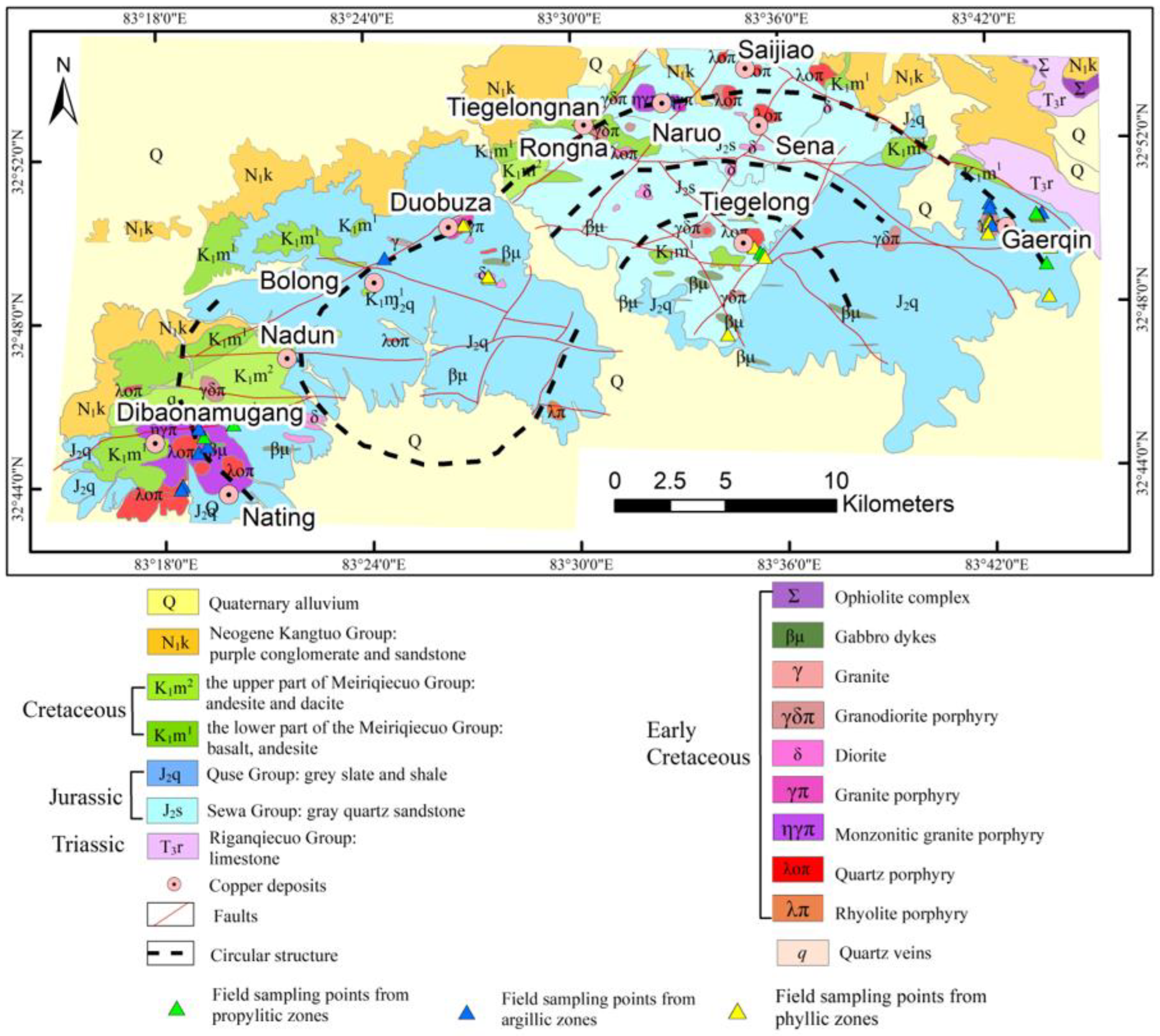
2. Geological Setting

The study area is situated in the Duolong ore district in Tibet, China, covering approximately 324 km2. Tibet consists of several terranes that were progressively accreted onto the southern margin of Eurasia during the Paleozoic and Mesozoic. These terranes are separated by a series of suture zones that are defined by ophiolitic fragments and mélanges [32].
The Duolong ore district is located in the western part of the Bangong Co-Nujiang metallogenic belt. The origin and evolution of this region are mainly controlled by the ocean–continent subduction system between the Bangong–Nujiang Tethyan Ocean and the South Qiangtang terrane [33]. The Middle-Lower Jurassic Sewa group (MLJS) and the Middle Jurassic Quse group (MJQ) are largely exposed in the area, and both are important ore-containing strata in the study area [34].
This area has experienced a long history of tectonic changes and has undergone geological actions such as extensional fissures, compression, and reduction. Faults are developed there, whose trends are mainly east–west, northwest, and northeast (Figure 1) [33].
Except for the Tiegelongnan (Rongna mine section) and Dibaonamugang, which are porphyry–epithermal complex copper deposits, other deposits, such as Bolong and Duobuza, are all PCDs. The porphyry-epithermal deposits have a symbiotic and transitional relationship with the porphyry deposits, appearing together in space [3]. Studies of the Duolong district [35,36,37] have shown that all the deposits in the area have the same source of metallogenic materials that originate from the same magma source. Although these two types of deposits are produced at different locations in the vertical direction, they are the products of the same magma-hydrothermal system under different depths and physical and chemical conditions. These deposits constitute a complete porphyry-epithermal metallogenic system, which is an integral part of the porphyry metallogenic system. Although the alteration zonation of different PCD regions is slightly diverse, they generally conform to the following pattern [38]: from the inner outwards, the concentric alteration zones successively follow the potassic-silicate zone, the phyllic zone, the argillic zone, and the propylitic zone. The phyllic and argillic zones are overlying. The main altered minerals in the central potassic-silicate zone are quartz, potassium feldspar, sericite, biotite, chalcopyrite, bornite, and pyrite; the main altered minerals in the phyllic zone are sericite, quartz, chalcopyrite, pyrite, and magnetite; the main altered minerals in the argillic zone are kaolinite and alunite; and the main altered minerals of the propylitic zone in the margin of the porphyry deposit are chlorite and epidote.

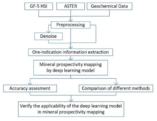
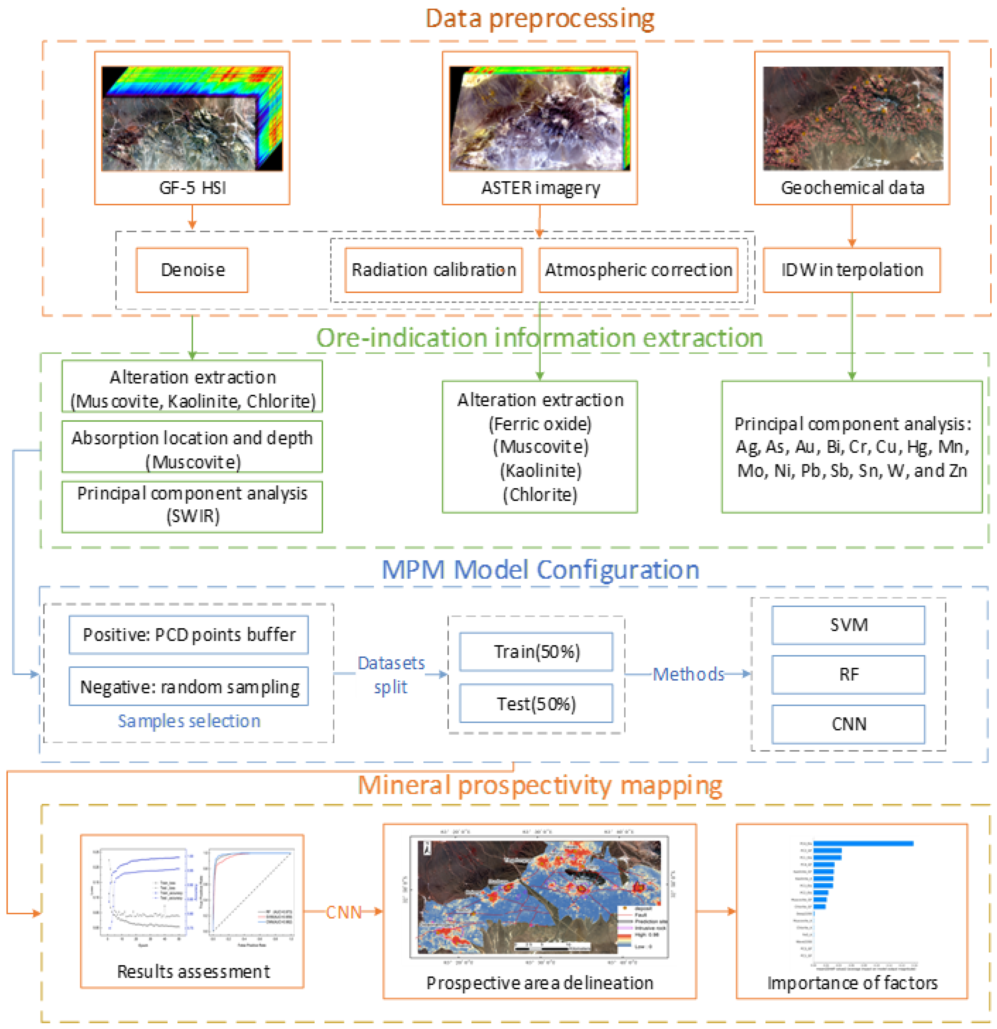
3. Materials and Methods

The experimental process consists of four parts: data preprocessing, ore-indication information extraction, mineral prospectivity mapping, and prospective area delineation, as shown in Figure 2.

3.1. Materials and Data Preprocessing

The remote sensing data used in this study were mainly Gaofen-5 (GF-5) hyperspectral images (HSIs) supplemented by ASTER multispectral images. The regional geochemical data and related explanatory materials were also obtained.

3.1.1. Preprocessing of GF-5 HSIs

The GF-5 satellite has been used since 2019 and is a hyperspectral satellite with a high spectral resolution in the visible–shortwave infrared range (SWIR). It can provide a reliable source for future large-area practical applications. The GF-5 Advanced Hyperspectral Imager is a 330-band imaging spectrometer with a 30 m spatial resolution covering the 400–2500 nm spectral range. The visible and near-infrared (VNIR) spectral resolution is 5 nm, covering 390–1029 nm with 150 bands; the SWIR spectral resolution is 10 nm, covering 1005–2513 nm with 180 bands [39].
The preprocessing of the GF-5 L1 data mainly includes the following steps: bad-band removal, radiometric calibration, and atmospheric correction. The preprocessing of GF-5 HSIs was completed on ENVI 5.3.
  • Bad-band removal
The GF-5 spectral ranges of the 145–150 band in VNIR and the 151–153 band in SWIR overlap. Because 145–150 bands have the advantage of a high signal-to-noise ratio (SNR), 145–150 bands were retained. Part of the bands located in the water vapour absorption zone leads to radiant energy affected by the strong absorption of water vapour, resulting in real ground information loss. Bands 191–200 and 246–262, which are greatly affected by water vapour, were removed. Ultimately, 300 effective bands of GF-5 HSIs were reserved, including the 1–150, 154–190, 201–245, and 263–330 bands.
2.
Radiation calibration
This step converts the digital number value on the image into the radiance value. The gain and offset values can be obtained from the GF-5 HSI header files. The band interleaved by line (BIL) was set as the output interleave, and the scale factor was set to 0.1.
3.
Atmospheric correction
Owing to the scattering and absorption of the atmosphere, the original digital remote sensing imagery has radiation distortion when electromagnetic radiation is transmitted. Remote sensing imagery without atmospheric correction cannot be directly applied to mineral mapping; otherwise, it will cause errors in the results. In this study, the FLAASH model for atmospheric correction [40] was used.
4.
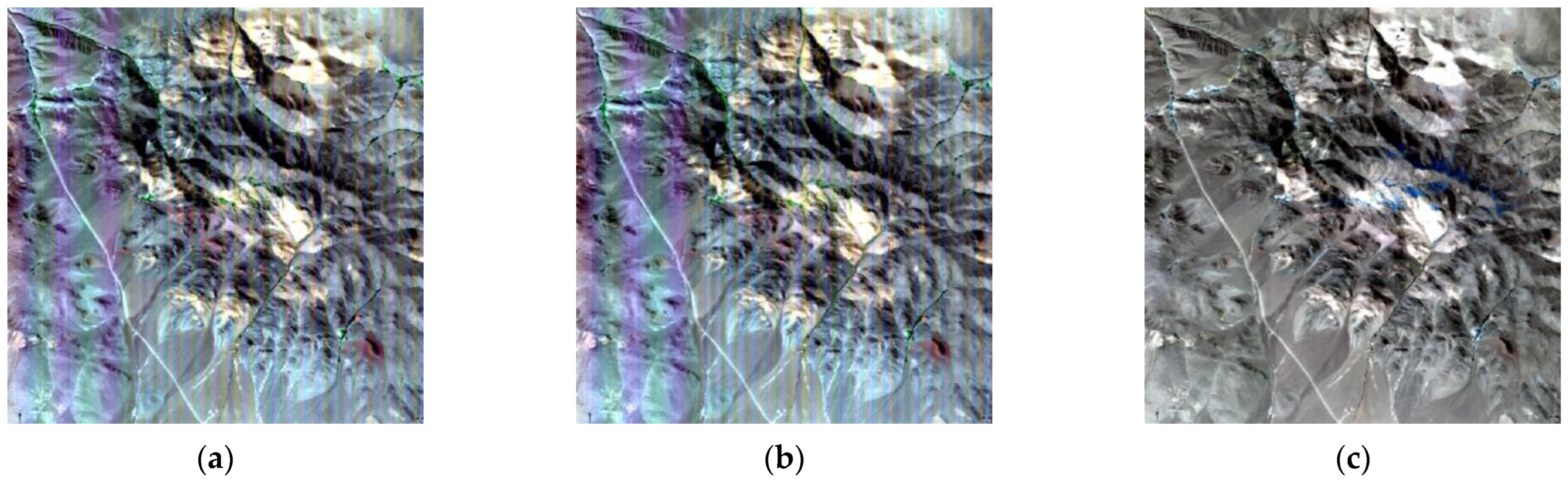
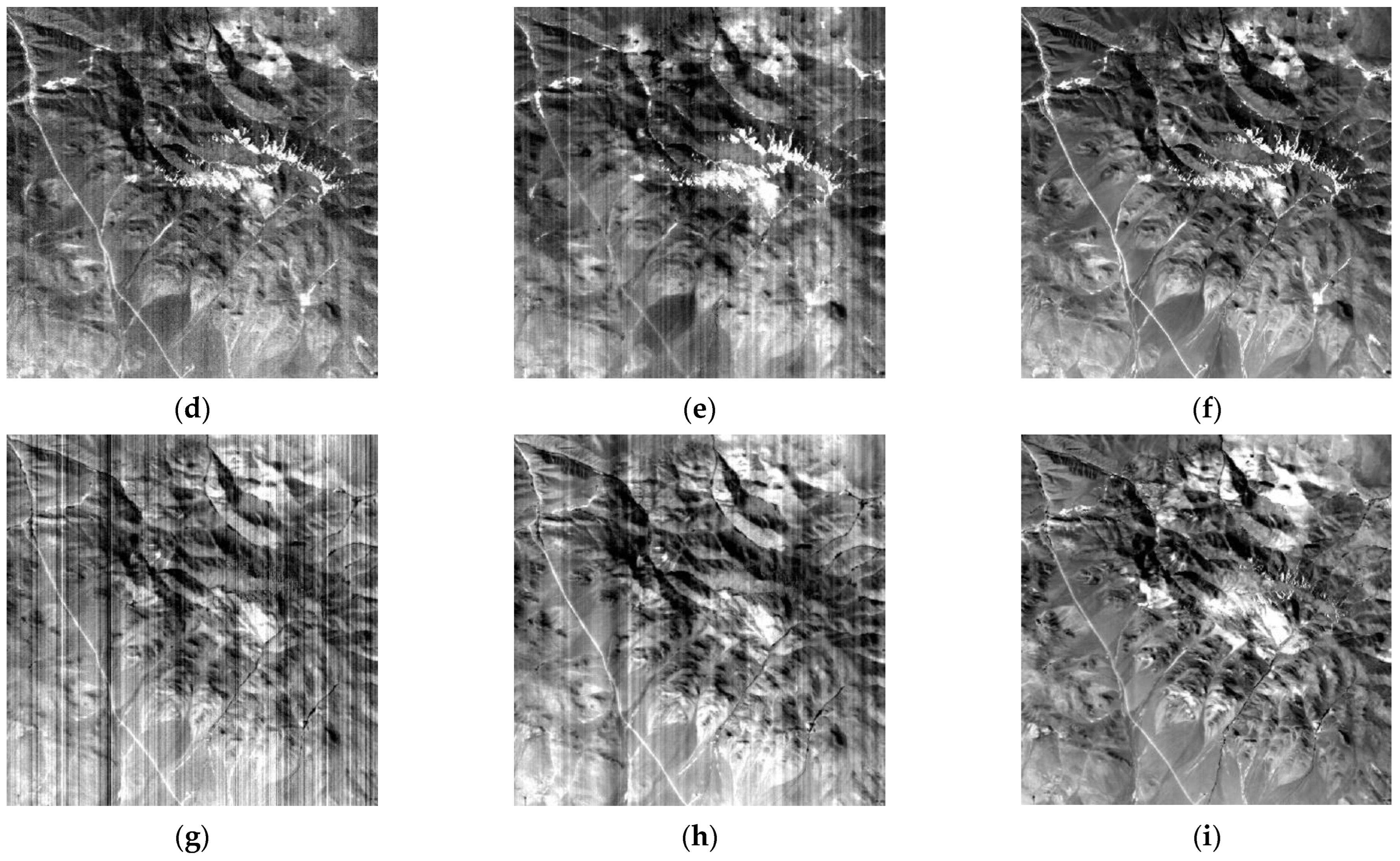
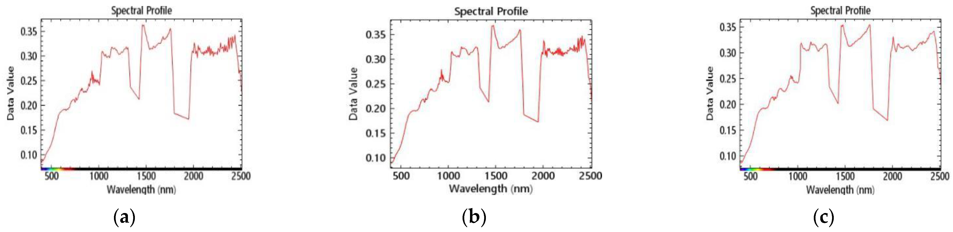
Denoise via Subspace-Based Nonlocal Low-Rank and Sparse Factorization
After the first three steps, severe noise remains in the GF-5 data, influencing the subsequent MPM tasks. Aiming at the most important prior information of HSI denoising, i.e., spectral band correlation and spatial nonlocal similarity, a regularization model via subspace-based nonlocal low-rank and sparse factorization (SNLRSF) was established to denoise HSIs [41].
When the HSIs have mixed noise, the regularization model separates the sparse noise and Gaussian noise to establish an HSI denoising model. Clean HSI spectral bands have a strong spectral correlation, so the HSI denoising model can be written by spectral global low-rank factorization as follows:
Z ^ , S ^ = arg min Z , S 1 2 Y - E Z - S F 2 + λ 1 F 1 ( Z ) + λ 2 S 1 s . t .   E T E = I k
where Y is a 2-D matrix, that is reshaped from an observed HSI cube; E denotes the basis of the subspace in which E is orthogonal, i.e., E T E = I k , with I k representing the identity matrix of the size. The matrix Z denotes the representation coefficient with respect to E ; S denotes sparse noise; · F 2 represents the Frobenius norm; and parameters λ 1 and λ 2 ≥ 0 balance the contributions of the three terms to the result.
Eigenimages have two important properties that benefit the image-denoising task [42]: the nonlocal self-similarity of each eigenimage, and the correlation among the eigenimages. A spatial nonlocal low-rank decomposition was selected to exploit the abovementioned two properties. The HSI denoising model with subspace-based nonlocal low-rank and sparse regularization can be reformulated as:
C ( . , . ) E ^ , Z ^ , L ^ , S ^ = arg min E , Z , L , S 1 2 Y - E Z - S F 2 + λ 1 i 1 δ i 2 i Z L i F 2 + κ ( L i ) + λ 2 S 1 s . t .   E T E = I k
where L i represents the clean 3-D tensor, κ ( L i ) denotes the sum of the singular values of matrices flattened by the tensor, δ i 2 is the noise variance of the 3-D tensor used to normalize the F-norm data fidelity term, and i is a binary operator to withdraw nonlocal similar overlying 3-D patches. The model was composed of three parts: spectral low-rank factorization for HSIs in subspaces; nonlocal low-rank factorization for characterizing spatial nonlocal self-similarity along with the high correlation among eigenimages; and the l 1 -norm sparse term for considering sparse noise.
After all preprocessing, the entire image was clipped to an appropriate size according to the study area to facilitate subsequent research.

3.1.2. ASTER Preprocessing

ASTER, an advanced multispectral imager on the Terra satellite, covers 14 bands from VNIR (520–860 nm), and SWIR (1600–2430 nm) to the thermal infrared range (TIR) at ground resolutions of 15 m, 30 m, and 90 m respectively. Each ASTER scene covers an area of 60 × 60 km. In this research, two AST_L1T level products were used, which were subjected to orthorectification and terrain-accurate correction. ASTER preprocessing technology is relatively mature and forms a standardized process [43]. This research mainly utilized VNIR-SWIR band data. The VNIR-SWIR datasets were resampled by using the nearest neighbour resampling method and stacked into a nine-band file so that all bands had the same 15 m pixel size to preserve the spatial features provided in the VNIR bands. The preprocessing process was carried out on the ENVI 5.3 platform, which mainly includes radiometric calibration and FLAASH atmospheric correction, similar to GF-5 preprocessing.

3.1.3. Geochemical Data Preprocessing

Based on a 1:50,000 stream sediment geochemical survey in the Duolong ore district in 2008, 1748 samples in the study area were selected for preprocessing. The samples were analysed by the Southwest Metallurgical Geological Testing Center. Each point selects 15 trace metal elements, such as Ag, As, Au, Bi, Cr, Cu, Hg, Mn, Mo, Ni, Pb, Sb, Sn, W, and Zn. The impacts of compositional or stoichiometric closure constraints are usually neglected because of the low concentrations of these trace elements [44]. The inverse distance weight (IDW) (a two-dimensional interpolation function for irregularly spaced data) is a common spatial interpolation method, that weights the distance between the interpolation point and the sample point as the weighted average, and the sample point closer to the interpolation point gives a greater weight. The original geochemical data employed IDW to interpolate 15 layers with a 100 m × 100 m grid size, performed in ArcGIS 10.5.

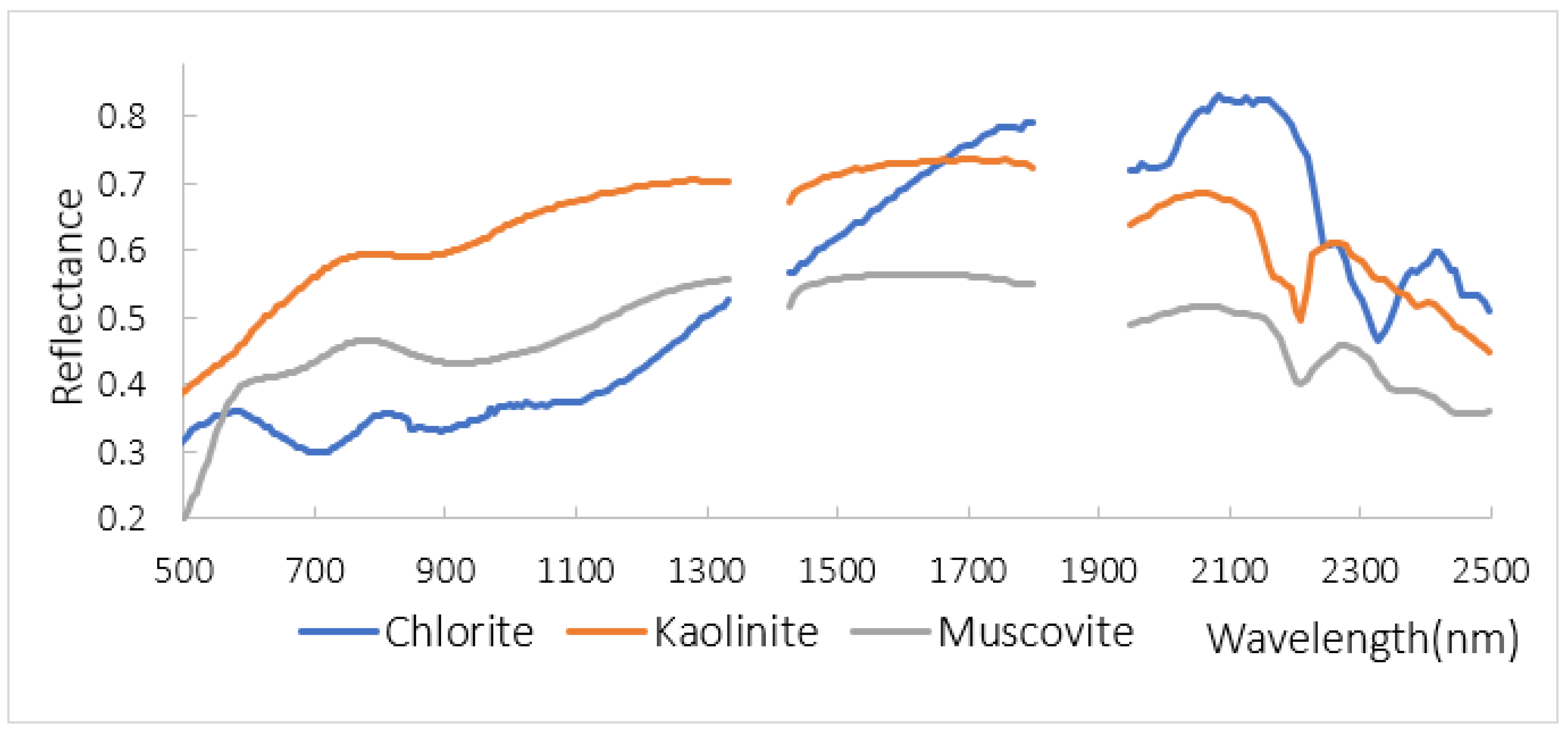
3.2. Hydrothermal Alteration Mineral Mapping Methods

3.2.1. Spectral Properties of Hydrothermal Alteration Minerals

Most alteration minerals have absorption features in the wavelength range of 2050–2450 nm. They can be identified by using features such as the location, width, and depth of the absorption peaks [45]. In this study, porphyry copper ore bodies primarily occur in the potassic and phyllic zones characterized by chalcopyrite and pyrite [34]. The main alteration minerals, including muscovite, kaolinite, and chlorite, were collected; their spectral curves, selected from the USGS mineral library, are shown in [46].
The reflectance spectra of chlorite, as a typical propylitic alteration mineral, exhibit Mg-OH and Fe-OH absorption features, whose main absorption peaks are centred at 2327 nm. Kaolinite, the indicator mineral of argillic alteration, displays an Al-OH group absorption position at 2209 nm and a secondary absorption peak at 2167 nm [11]. For phyllic alteration indexed by muscovite, Figure 3 shows an intensive Al-OH absorption at approximately 2200 nm. According to the different contents of Al, the location of the Al-OH absorption peak will shift in the longwave direction with decreasing Al content [47].

3.2.2. Endmember Extraction and Hyperspectral Unmixing via Sparse Autoencoder Network

Compared with multispectral imagery, HSIs have a lower spatial resolution, resulting in a pixel containing multiple mineral spectral information due to smaller mineral scales. Therefore, the prime process of mineral information extraction using HSIs is hyperspectral unmixing, which contains endmember extraction and abundance estimates [48]. We used the EndNet method to extract endmembers and estimate abundance. EndNet is constructed on a two-stage autoencoder network that is restructured by introducing additional layers and a projection metric (spectral angle distance in place of inner product) to realize optimization [49]. A novel loss function constituted by a Kullback–Leibler divergence term with spectral angle distance (SAD) similarity and additional penalty terms was renovated to better the sparsity of the estimates. This method, which can extract endmembers and estimate abundance in an unsupervised manner, has demonstrated excellent performance in hyperspectral unmixing.
An autoencoder is an artificial neural network that belongs to a three-layer, fully connected structure, including an input layer, a hidden layer, and an output layer. The input layer and the hidden layer compose an encoder, which converts the high-dimensional raw data to a low-dimensional space through mapping to obtain the data feature representation. The output layer and the hidden layer constitute a decoder, which restores the feature representation to reconstructed data [50]. Traditional autoencoders are less stable because the inner product of the input data is not adequately discriminative, which may lead to abundance estimation error. The standard Euclidean distance reorganization term used as the chief penalty function for minimizing the estimation error may lead the solution to fall into a local minimum.
To solve the above problems, first, the rectified linear unit (ReLU) function was used as the activation function in the encoder layer instead of the logistic function, which makes the trained network exhibit sparsity. A normalization layer was introduced before and after the ReLU function to increase the robustness of the network. Using SAD instead of the inner product can more easily separate endmembers from other interfering information [51]. The loss function can be written as:
L = λ 0 2 x x ^ 2 2 λ 1 D K L 1.0 C x , x ^ + λ 2 z 1 + λ 3 W e 2 + λ 4 W d 2 + λ 5 ρ 2
where C ( . , . ) denotes the normalized SAD score between the initial and the reconstructed data; D K L is a Kullback–Leibler divergence term to maximize the SAD score distributions; z 1 is a regularization term; and ρ and λ are trainable parameter sets.

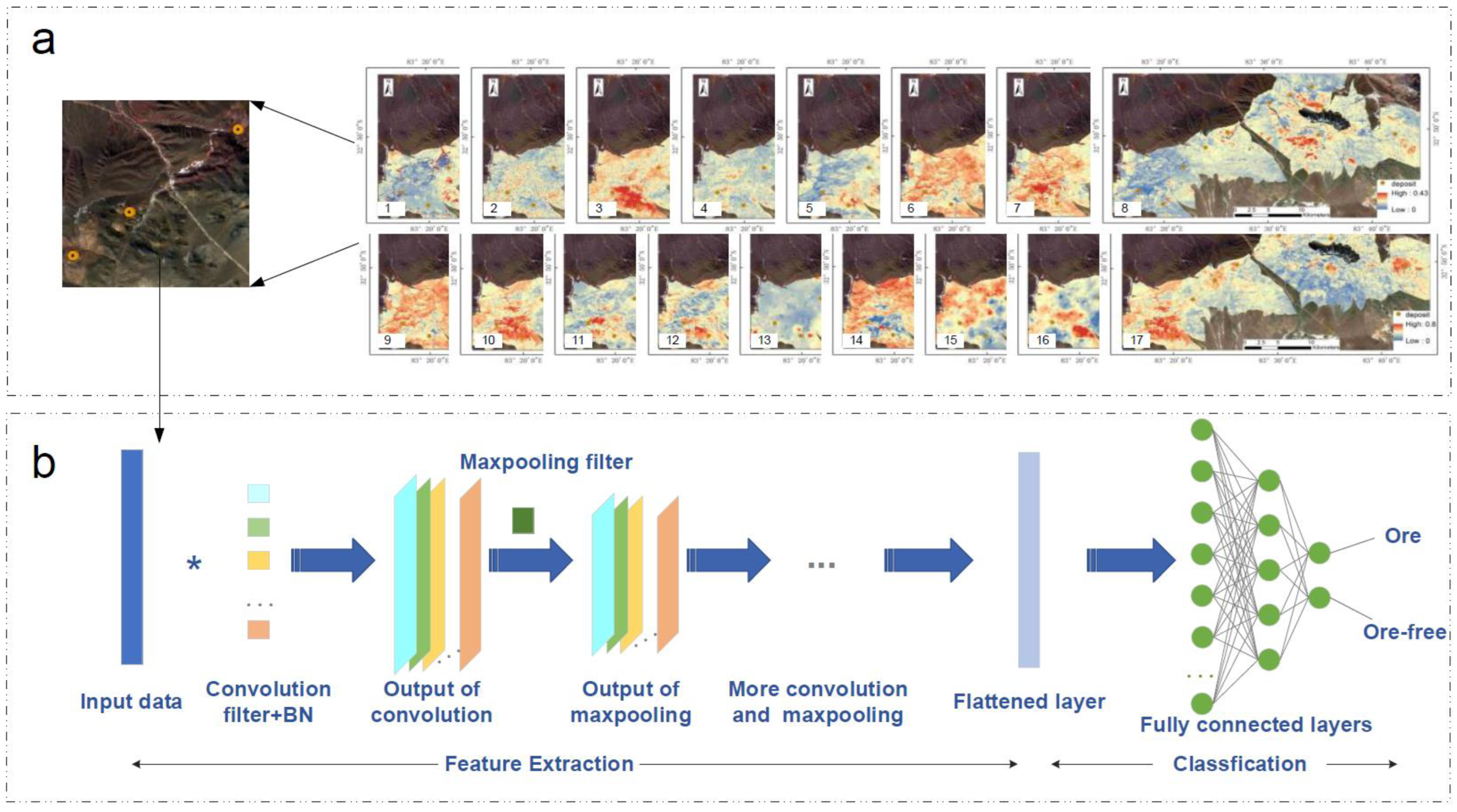
3.3. Deep Learning Model: CNN

DL neural networks can adaptively extract simple features from the original data and then extract deep features from the simple features. Layer-wise learning can reduce the dependence on features for a simple neural network [52]. CNN is a neural network model with a convolutional structure consisting of an input layer, a hidden layer, and an output layer. The hidden layer contains convolutional layers, pooling layers, and fully connected layers. Compared with traditional metallogenic prediction methods, one-dimensional (1-D) CNN processes can directly process raw data to achieve “end-to-end” classification, which is more flexible and less dependent on expert knowledge. The designed 1-D CNN model for MPM is shown in Figure 4. The feature data are converted into a 1-D array as the input layer. The convolutional layers employ a randomly initialized kernel (also called a filter) to perform a convolutional operation, which calculates the dot products to obtain a new feature dataset between the kernel and the input data. The activation function of the convolutional layer is the nonlinear ReLU function [53]. The pooling layers are also kernel-based processes using a moving kernel to extract the maximum value of the data overlapped by the kernel. Through convolution layers paired with pooling layers, the input data are propagated to draw out features. The drawn feature maps are sent to the flattened layer, which is used to flatten features to fit into the fully connected layers. The output of the fully connected layers is transmitted to the last layer, which applies the softmax function to reach the predictive probability and outputs a binary prediction. To enhance the generalization of the network, dropout layers are added to skip some samples with a certain probability, which can reduce the dependence on some local features [54]. In addition, batch normalization (BN) layers are introduced to avoid network training overfitting [55] and enhance the distribution consistency between the test set and the training set.

4. Results

4.1. Denoised GF-5 HSIs

The SNLRSF method was employed to denoise the GF-5 image compared with the traditional method: minimum noise fraction (MNF) [56]. The MNF method was employed to rotate the original GF-5 image to choose the first 30 bands. The former 30 bands were retained for the inverse MNF rotation to obtain hyperspectral imagery with 300 bands. The noisiest parts of GF-5 are in the SWIR band, so false colour bands (R:269, G:299, B:317) were chosen to show the denoised effect. Three bands were integrated into 3-D imagery after different denoising methods in the GF-5 dataset, as shown in Figure 5a–c. Figure 5d–i shows denoising results on band 1 and band 330, respectively. It is obvious that only part of the Gaussian noise can be removed through MNF, with much stripe noise remaining. Compared to MNF, the SNLRSF method achieves improved visual quality and retains more detail, effectively removing the stripe noise and salt-and-pepper noise. The essential reason is that spectral low-rank and spatial nonlocal self-similarity of HSIs are both considered in the SNLRSF method.
Furthermore, a point of the image was selected to present the spectral curve before and after denoising (the bands in the ranges of 1334–1426 nm and 1798–1948 nm were removed in the preprocessing), as shown in Figure 6. The spectral curve of the original image exhibits rapid fluctuations, and the SNR is low. Via the MNF method, the curve shows no obvious change, and only the sawtooth is partially reduced. Clearly, the spectral curve processed by the SNLRSF method is relatively smooth. Compared with the original image, the peak of absorption and reflection at this point did not shift, indicating that the SNLRSF method can efficiently reduce the noise on the basis of retaining most of the structural information of the raw image.

4.2. Ore Indication Information Extraction Based on Multisource Data

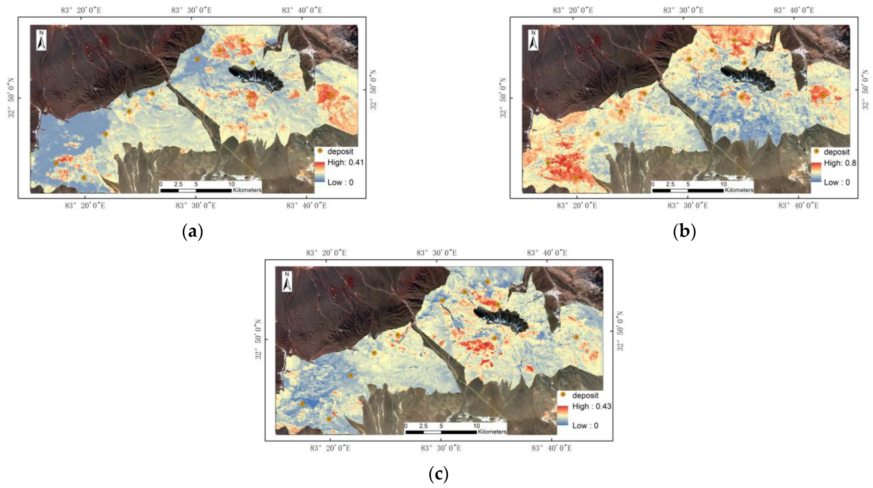
4.2.1. Ore Indication Information Extraction Based on GF-5 HSIs

  • Alteration mineral mapping
Based on the 300 bands of the preprocessed GF-5 HSIs, we used EndNet to attain the main altered mineral and abundance estimates. The USGS spectral curves were used as the endmember spectra in the EndNet processing. In Tiegelongnan and Dibaonamugang, the muscovite distribution (Figure 7a), an indicator of the phyllic zone, is less than the kaolinite distribution. Argillization, a broad developing alteration type in Duolong, primarily displays intensive kaolinization [57], which is distributed in all deposits shown in Figure 7b. The distributions of kaolinite and muscovite overlap in some areas, such as Tiegelong and Gaerqin. The representative mineral of the distal alteration zone, propylitic, is essentially chlorite. The wall rock surrounding the ore body in Duobuza and Tiegelong is a widely propylitic zone distributed outwards of the argillic and phyllic zone in a zonal-circular pattern (Figure 7c).
2.
Determination of the Absorption Location and Depth
Along with the spectral features of the alteration mineral muscovite in Duolong, the feature absorption peak position and maximum absorption depth of each pixel were calculated in the spectral range of 2190–2210 nm to embody the position shift of the global absorption feature and the changing trend of absorption depth. The absorption position and depth are obtained by using the least square simulated spectral curve after continuum removal [58] and then using the second derivative. Most of the absorption peaks of deposits are in the middle or short wavelength (Figure 8a), and the absorption depth is deeper than that in the ore-free zone (Figure 8b).
3.
SWIR Processing Results
Muscovite, kaolinite, and other alteration minerals are usually affected by surface physical processes [59], whose characteristics are less noticeable in the VNIR but obvious in the SWIR of 2000–2450 nm [60]. To reveal the SWIR information, 55 bands (band: 269–323, wavelength range: 1999–2454 nm) with typical features of the preprocessed GF-5 HSIs were selected to perform the principal component analysis (PCA) method. Seven principal components (PCs) were extracted by the PCA method, but the last three PCs were all displayed as disordered noise. Therefore, the first four principal components (PCs) were selected for subsequent analysis (Figure 9). The cumulative contribution of the four PCs reached 99.99%, preserving the characteristic SWIR information to the greatest extent.

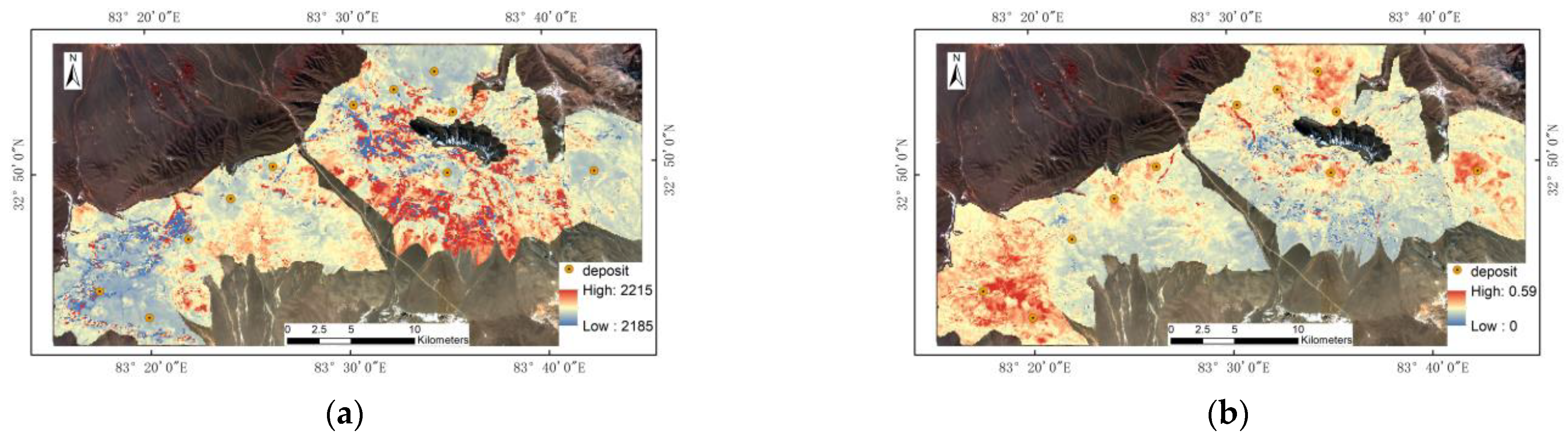
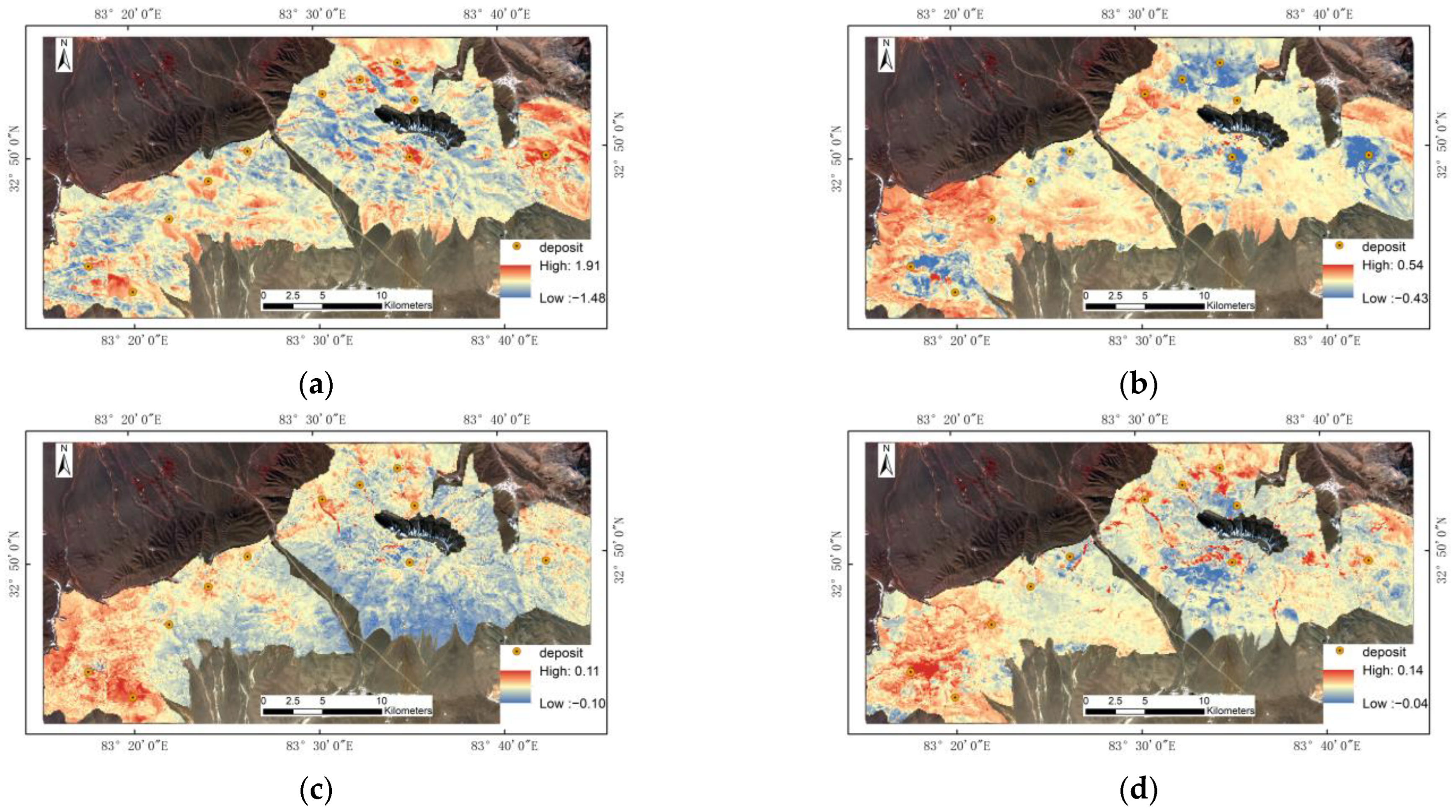
4.2.2. Ore Indication Information Extraction Based on ASTER

The BR and RBD methods were utilized for ASTER imagery to map the hydrothermal alteration minerals related to the alteration zones of Duolong. The following formulas (Table 1) were used to extract the corresponding mineral information [61,62], as shown in Figure 10. The ferric oxide is widely distributed in the argillic and propylitic zones of Duolong. The distributions of the other three alteration minerals extracted from ASTER data are similar to those from GF-5 HSIs. There is obvious local enrichment of muscovite, such as in the Tiegelong and Naruo areas, and kaolinite is widely distributed, especially in the Dibaonamugang, Tiegelongnan, and Saijiao areas. The kaolinite of the argillic alteration mainly coexists with muscovite in Tiegelong, Bolong, and Duobuza. Chlorite extracted from ASTER is more widely distributed than GF-5 HISs in Dibaonamugang and Tiegelongnan.

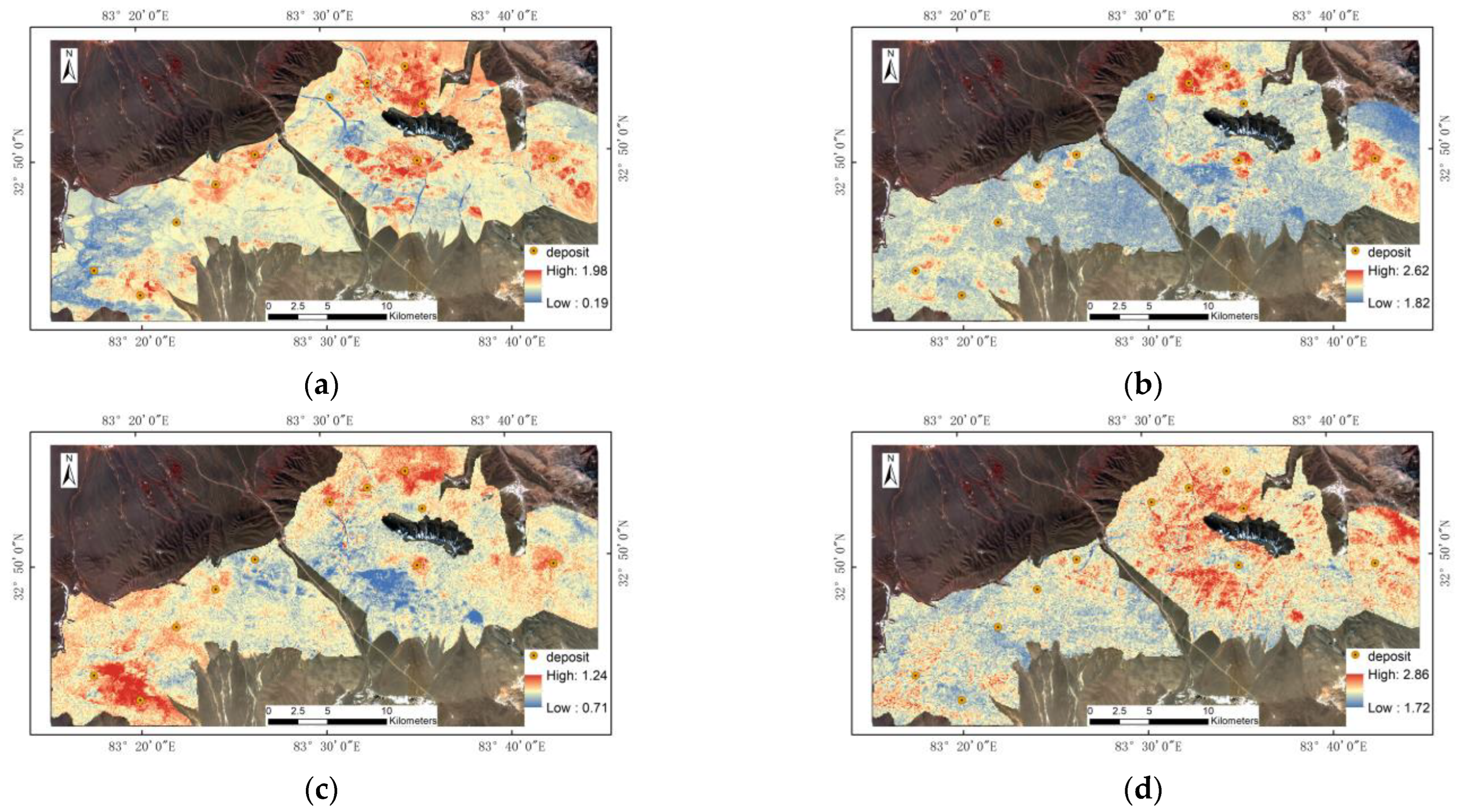
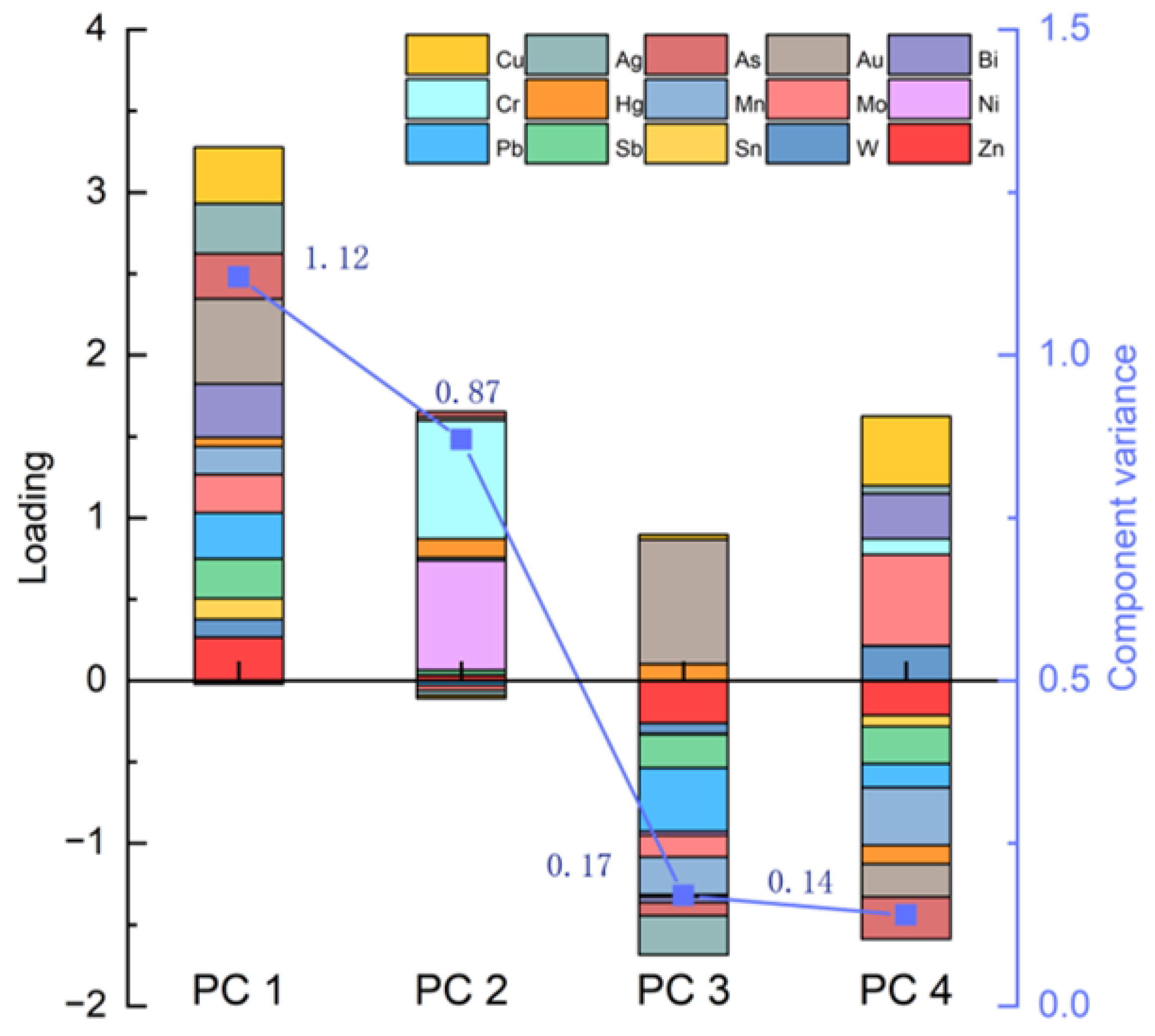
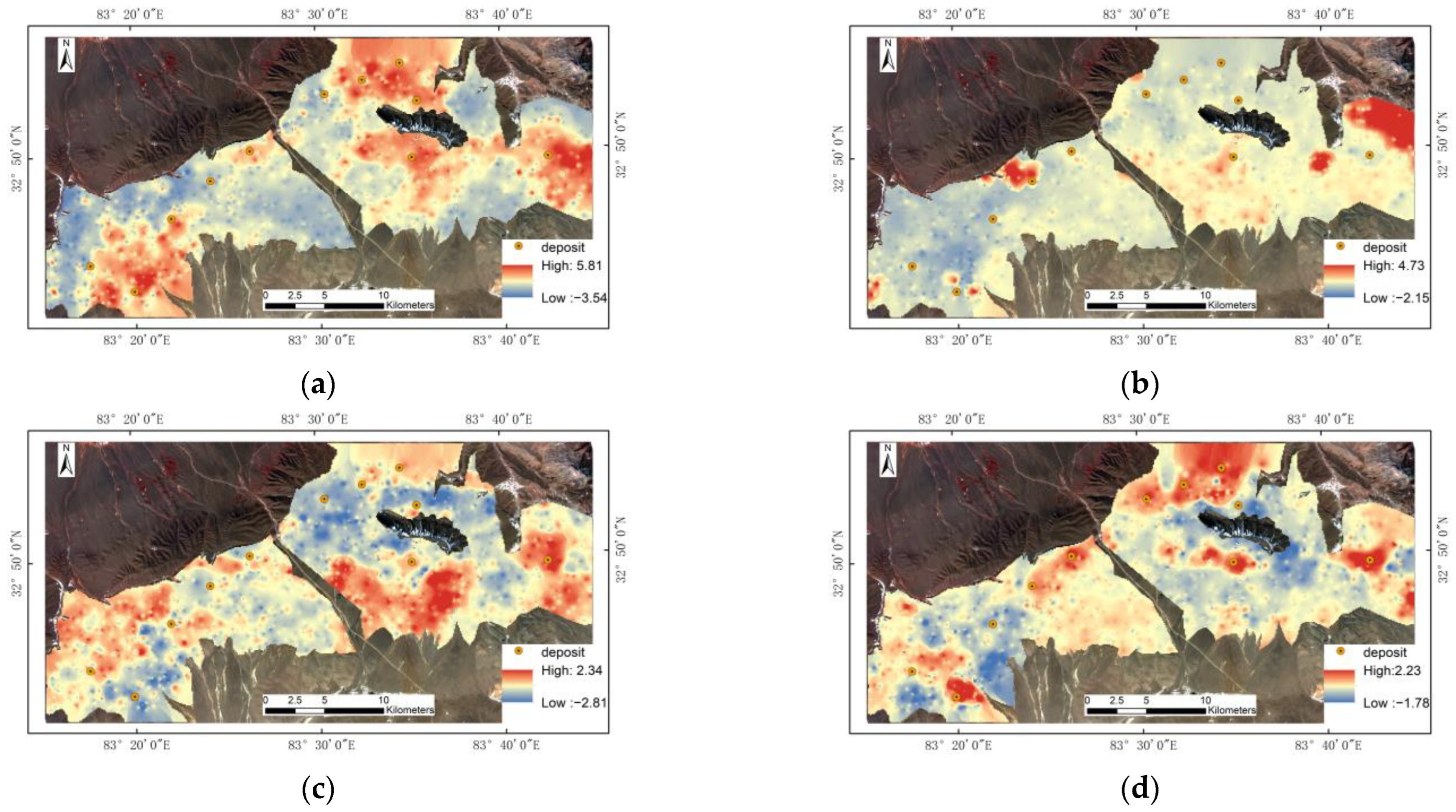
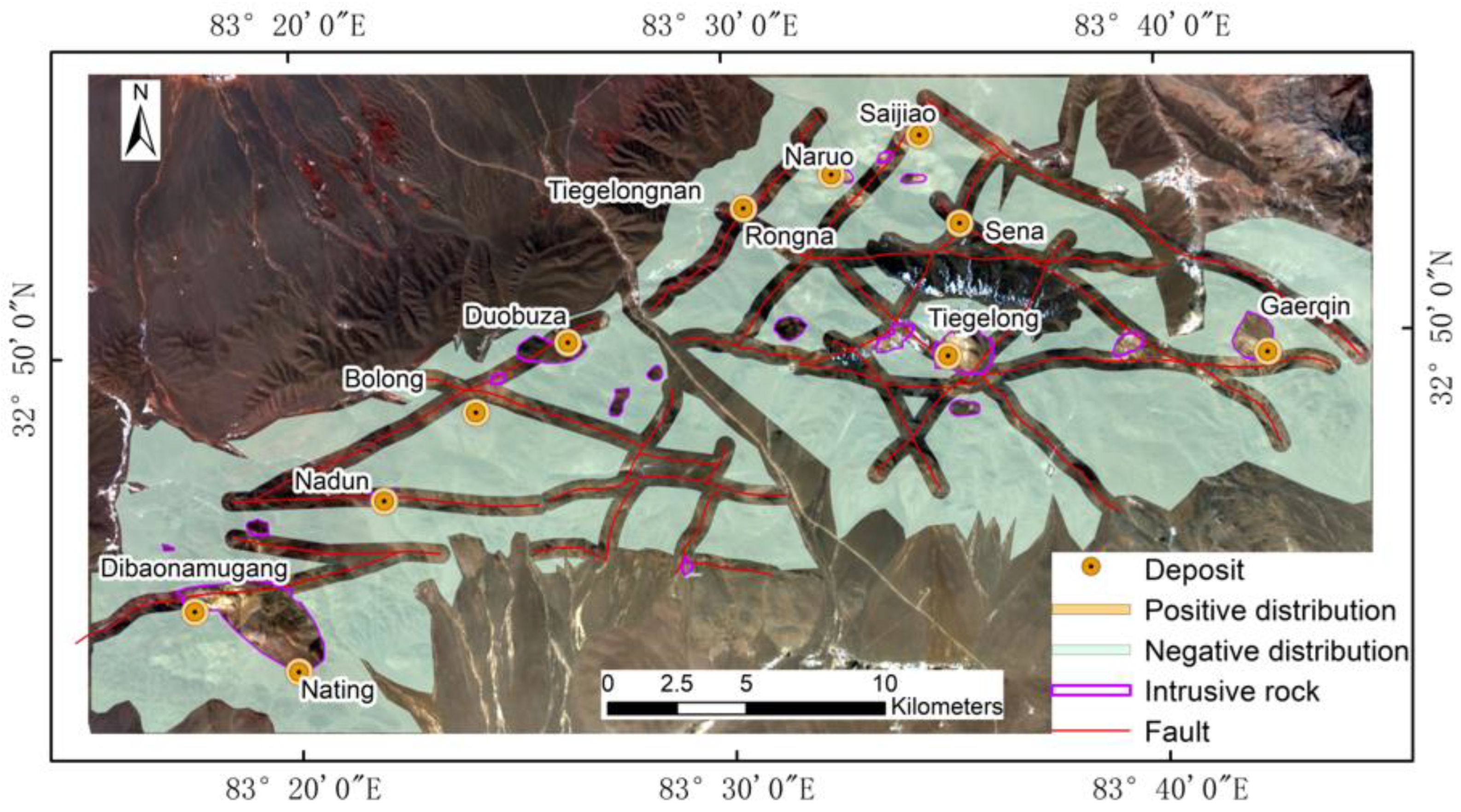
4.2.3. Ore Indication Information Extraction Based on Geochemical Data

The PCA method was performed on the 15 elements interpolated by the IDW to reduce the dimensions of the geochemical elements. Before the PCA process, the data were logarithmically transformed and standardized. Seven PCs were extracted by the PCA method. The first four PC factors explain 85% of the total variance of the original 15 elements. The last three PCs contain less than 3% original information. We chose the first four PCs, taking into account the computational cost. Figure 11 shows the loading and component variance of each PC. The first PC contains 41% of the information, Au exhibits the largest loading, and Cu takes second place. The second PC contains 32% information, Cr has the largest load, and Ni is number two. The third PC contains 6% information, and Au demonstrates the largest load. The fourth PC contains 5% information, and Mo is the largest, followed by Cu. Figure 12 shows the distribution of different values of each PC.

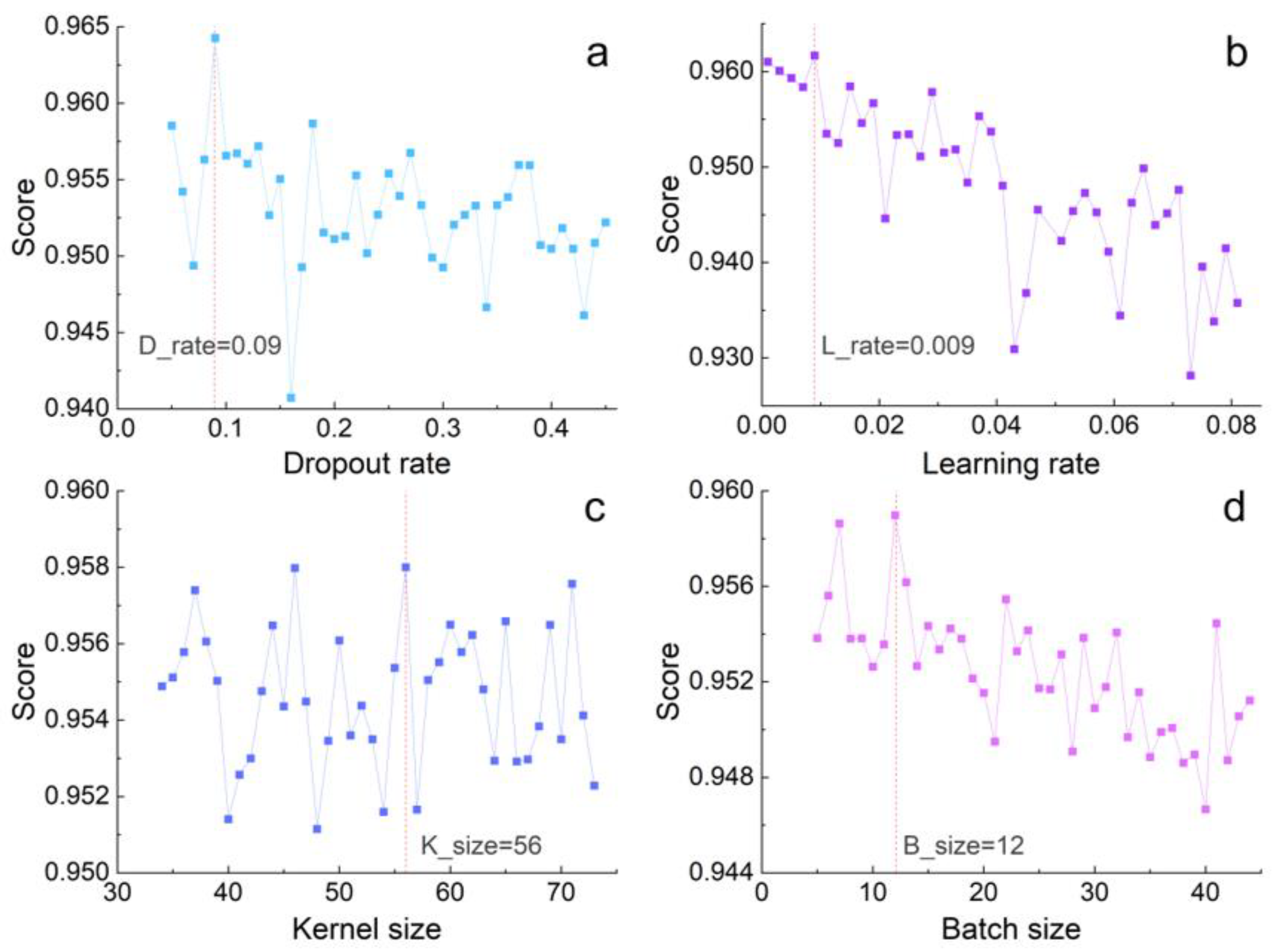
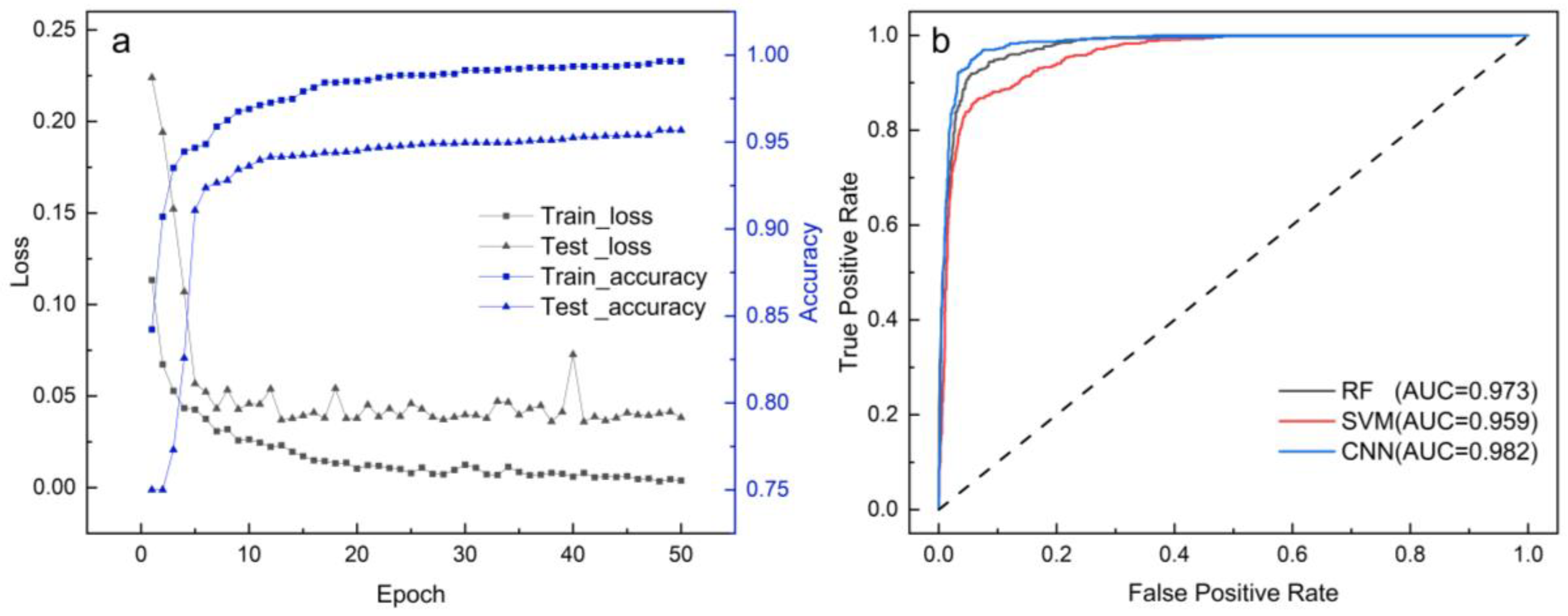
4.3. MPM Model Configuration and Classification Results

For the 11 copper deposits as positive samples in Duolong, the number of pixels of known deposits, namely, 11, is considerably low compared with the total number of 100 m by 100 m pixels in the study area. It will bias the model and impede the generalization ability of deep learning algorithms. To meet the requirements of large-capacity training samples for DL, using data augmentation methods for generating positive samples is accessible [63]. Data augmentation in geology, including buffering [64], XGBoost [65], and random-drop data augmentation [66], has been successfully applied for generating additional positive samples in MPM. By 500-metre buffering, 11 copper deposits can acquire a total of 868 positive samples. There are two strategies from the geological viewpoint for selecting negative training samples, including random locations [67] and low-probability areas [68]. According to the local metallogenic conditions [69] and known mineral occurrences, negative samples should be randomly selected outside the favourable metallogenic area, including copper deposits, intrusive rocks, and faults. Figure 13 shows the distribution of positive and negative samples. To alleviate the overfitting phenomenon due to deposits accounting for a small proportion of the predicted area, the negative samples are 3 times the positive samples, namely, 2604 negative samples. The training subset and the test subset contain equal quantities of samples, according to a ratio of 1:1.
Predictors were employed as determining factors for predicting mineral potential. Based on the genetic model and controlling factors of Cu mineralization and according to the above-extracted ore indication information, 17 evidential maps involving remote sensing and geochemical information were employed as predictor variables. Nine predictor variables were from HSI images, consisting of three extracted alteration minerals, the maximum absorption depth and wavelength position in the 2185–2115 nm spectral range, and the first four PCs obtained after the PCA procedure for the 55 SWIR bands of GF-5 HSIs. Four predictor variables were derived from ASTER images and are alteration information extracted by BR or RBD methods. The spectral resolution of GF-5 HSIs is high compared to ASTER data, which have a low spectral resolution but a high SNR. The multiscale information complements each other, which is conducive to a comprehensive reflection of the ground features. Four predictor variables were the first four PCs of 15 geochemical elements after the PCA process.
Different hyperparameters in the CNN model have an impact on the classification performance. Four factors, namely, dropout rate, learning rate, kernel size, and batch size, were considered in this study. The epoch was set to 50, the X-axis was the independent variable, and the other hyperparameters were kept unchanged. Figure 14 shows the influence of selecting diverse hyperparameters on the final accuracy. The parameters corresponding to the highest scores were obtained; that is, the dropout rate was 0.09, the learning rate was 0.009, the kernel size was 56, and the batch size was 12 to obtain the best performance.
The CNN model trained by the optimal hyperparameters outputs the prediction. For comparison, traditional ML models, SVM and RF, were utilized. The three models exhibit different performances.
All the models can properly recognize the majority of known deposits in the study area. When epoch 50 is set, the loss and the accuracy level off in the training subset and test subset of the CNN model (Figure 15a). The accuracy of the CNN test subset is 0.956 and that of the training subset is 0.993 (Table 2). The RF accuracy comes next, with 0.937 and 0.998 for the test and training subsets, respectively. SVM models produce relatively worse predictions, with 0.931 for the training subset and 0.922 for the test subset. The accuracy of the training subset is higher than that of the test subset, especially for the RF model, which leads to overfitting. The CNN model takes second place. Although the accuracy of the training subset is slightly lower than that of RF, the prediction ability for unknown samples (test subset) is better than that of the other two models. The runtimes of the three models are quite different because the complexity of the CNN models is higher; CNN takes the longest time, followed by RF, and SVM is the fastest.
The delineation of the high-confidence area and predictive effectiveness of the model are vital for exploration applications such as MPM. Hence, predictive performance needs to be well assessed. The receiver operating characteristic (ROC) curve and AUC have been broadly utilized to assess the performance of classification models in MPM [70]. The more a ROC curve approaches the top left corner, the better the model performs. The performance of the three models was assessed by using ROC curves (Figure 15b). The ROC curve of the CNN model is the closest to the upper left corner. The AUC values show that CNN (AUC = 0.982) outperforms RF (AUC = 0.973) and SVM (AUC = 0.959). Many aspects have proven that the CNN metallogenic prediction model demonstrates the best performance, so the prediction results of the CNN model were selected to delineate the metallogenic prospect.

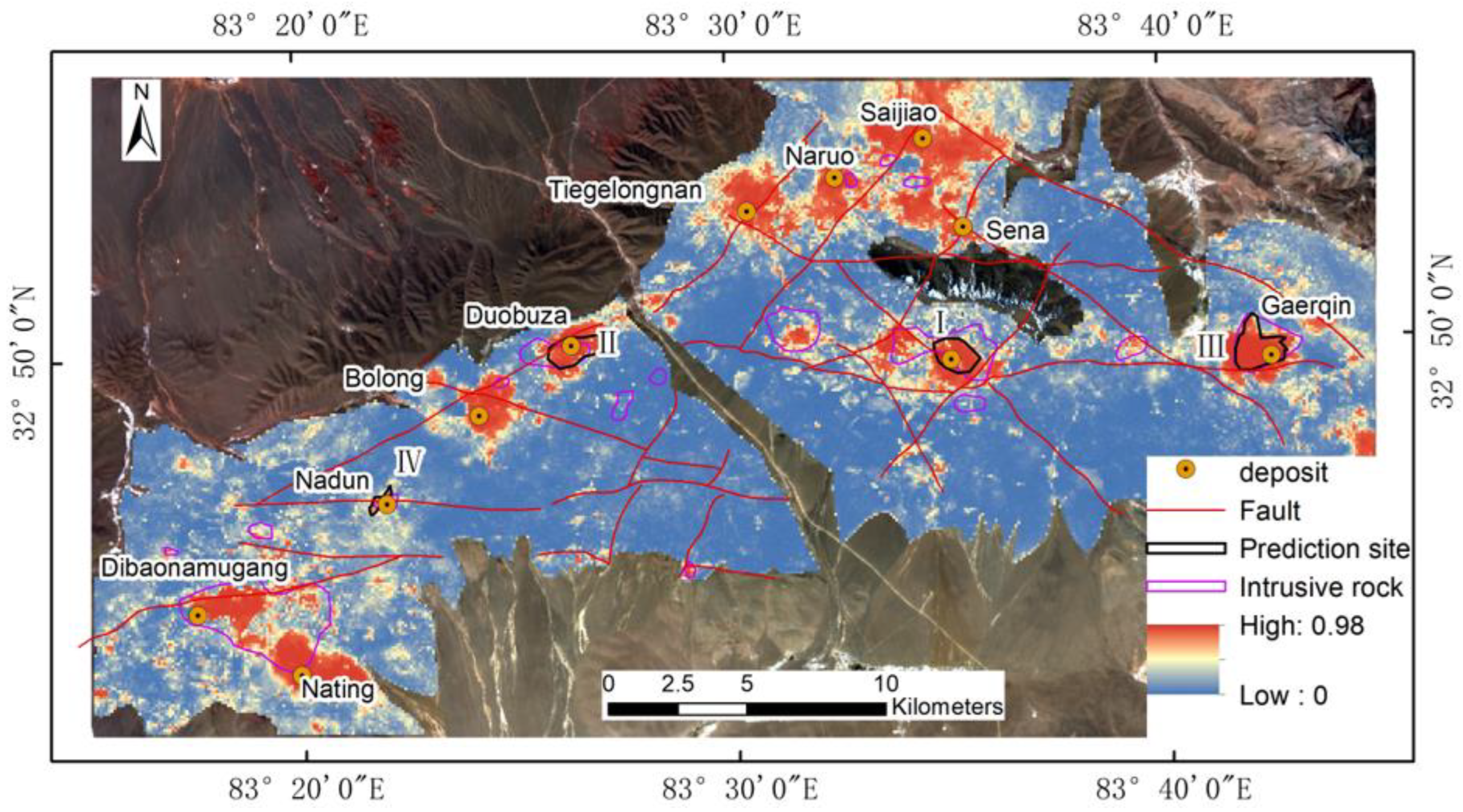
4.4. Mineral Prospectivity Map
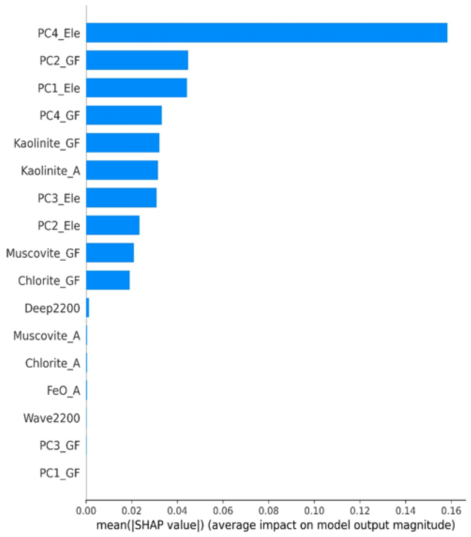
The CNN algorithm outputs the prediction probability at each grid that is embodied by a floating probability value fluctuating from 0 to 1. The DL model labels red grids with high values as potential sites that contain mineralization. The remaining blue grids are marked as ore-free regions without adequate prospecting potential. Based on the prediction results, according to the main structures, lithologies, and alteration zones, four metallogenic prospective areas are delineated, as shown in Figure 16 below.
All four prospects contain one known deposit and are in the predicted high-value area. In this area, obvious muscovite alteration zones overlap in the kaolinite zone, and the periphery of the prospective region is the chlorite alteration zone. The prospective areas are also located in the high-value area of Cu, where faults exist, and diorite porphyrite is exposed in the area. Prospect I is located in Tiegelong, and the exposed stratum is the MLJS group, where chalcopyrite-bearing diorite (Figure 17A), malachite, and pyrite sericite are found in the field. Prospect II is located in Duobuza, and the exposed stratum is the MLJS group. Malachite and azurite have been discovered in the field (Figure 17B), accompanied by pyrite sericite, silicification, and argillization. Prospect III is located in Gaerqin, and the exposed stratum is the MJQ group. Malachite, azurite, gossan (Figure 17C), and pyrite sericite have been discovered in the field. Prospect IV is in Naton, and the exposed stratum is the MLJS group. Malachite appears on the spot, and chalcopyrite can be seen in the quartz veins of the rock (Figure 17D).

5. Discussion

The ‘black box’ nature of DL models leads to an agnostic driver of the underlying process [29], which may hinder their implementation. To enhance the interpretability of DL models, Python’s SHAPs are utilized to interpret the individual predictions of the CNN model output using the SHAP library. SHAP values are calculated using a coalition game theory in which different coalitions of the feature set (i.e., numerous iterations of the models with all possible element combinations) are used to re-estimate the class prediction, and the difference in prediction when a specific feature is observed versus excluded is averaged. Feature importance scores were calculated by utilizing the SHAP library to show the relative importance of specific features during CNN model classification and to report the average scores (Figure 18). It is suggested that feature importance scores imply the significance of a feature to the model instead of the direct importance of the feature in nature. A key advantage of SHAP is that feature importance scores can be calculated for individual compositions.
The top five features that contribute the most to the model prediction score are the first and fourth PCs of geochemical elements, the second and fourth PCs of the SWIR band of GF-5, and the kaolinite alteration zone extracted from the GF-5 HSIs.
The scores of the first four PCs of the geochemical elements are high, and most of the deposits fall in the middle-high value regions of PC4 and PC1, showing a positive correlation. The top five largest positive loadings of elements in PC4 with the highest SHAP value are Mo, Cu, Bi, W, and Cr. The top five elements with the highest positive loadings of PC1 elements are Au, Cu, Bi, Ag, and Pb (Figure 19). These results coincide with the drilling results [71]; from the centre of mineralization outwards, the elements anomalously exhibit obvious zoning. Specifically, Mo-W-Bi-Sn is located in the centre of the ore body, and the middle zone combines Au-Cu-Sb; beyond the centre location and outwards are Ag-Pb-Zn. The combination of Mo, Bi, and W elements extracted from PC4 are all enriched elements in the centre of the ore body, indicating that the elements W, Mo, and Bi played a vital role in the prediction of porphyry copper ore. The Au, Cu, Ag, and Pb extracted by PC1 are mostly in the intermedial region of the ore body, and although the contribution score to the CNN model is lower than that of PC4, good performance is still achieved.
The PC2 and PC4 results of the GF-5 SWIR HSIs also play a large role in the predictive output of the model. Referring to Figure 9b,d, the incidence of PC2 and the ore point is a negative correlation. The deposits are mostly in the middle-high value area of PC4, which shows a positive correlation with PC4. The SWIR is roughly divided into four intervals: 1999–2091 nm, 2100–2185 nm, 2193–2319 nm, and 2328–2454 nm, and a 95% confidence ellipse (Figure 20) is circled. The bands with the largest positive loading of PC2 are in the 2328–2454 nm range, which mainly affects the ore-free area of the Duolong ore district. Chlorite and epidote, with main absorption peaks in the 2328–2454 nm range, are located on the periphery of the metallogenic alteration zone, generally not in the metallogenic centre. The bands with the largest positive loading of PC4 are mainly in the 2193–2269 nm range, showing a positive relationship because most deposits are located in the medium-high value areas of PC4. The diagnostic feature absorption of typical minerals in the inner-middle areas of the alteration zone, such as muscovite, kaolinite, montmorillonite, and illite [72], are all in the 2193–2269 nm range.
Comparing the influence of alteration bands extracted from two different remote sensing datasets on the prediction model, GF-5 HSIs demonstrate a better performance than ASTER when extracting the same alteration type. The argillic zone represented by kaolinite has the greatest influence on the output of the CNN model, followed by the phyllic zone represented by muscovite. The propylitic zone represented by chlorite exhibits the lowest influence. The reason is that argillic alterations usually overlap in the phyllic zone in the two porphyry–epithermal complex copper deposits of Tiegelongnan and Dibaonamugang [73]. Therefore, less muscovite is extracted from remote sensing images (Figure 7a), resulting in CNN models not extracting this feature very well. The argillic zone represented by the extracted kaolinite is distributed at each deposit, so the CNN prediction model correlates the argillic zone with the distribution of the deposits well. The propylitic zone is generally on the periphery of the ore site, not in the centre of mineralization, so the predicted high-value zone will not be there.

6. Conclusions

This research mainly focuses on GF-5 HSIs supplemented by ASTER and geochemical data, introducing the DL model into the field of metallogenic prediction. Predictive modelling of mineral prospectivity was accomplished in the Duolong ore district, Tibet. In this study, a synthetic MPM model was established, including GF-5 denoising technology, the comprehensive extraction of ore-indication information, and metallogenic prediction on the basis of the DL model. The DL model has shown strong potential in applications such as MPM. Based on integrating remote sensing imagery and geochemical data, the CNN model constructed in this paper has shown outstanding results. Although the accuracy of the training set is lower than that of RF, the test set reaches the highest accuracy of 0.956, showing better prediction ability for unknown samples. The known deposits are all situated in the middle-high value of the predicted outcomes.
According to previous research and fieldwork, four predicted places for favourable areas of ore prospecting were delineated, which are the key areas for the next porphyry copper deposit prospecting prediction.
Future research will focus on using DL algorithms to perform HSI denoising research based on spectral-spatial joint features. In addition, the interpretability of geological data in the DL models will be enhanced by the introduction of a knowledge-driven engine, and the lucid expression of evidential layers will be used to increase the usability of the DL algorithm.

Author Contributions

Conceptualization, Y.F. and L.J.; methodology, Y.F.; software, B.Y.; validation, Y.F.; formal analysis, Q.C. and Y.F.; investigation, Y.F. and L.J.; resources, L.J.; data curation, L.J.; writing—original draft preparation, Y.F.; writing—review and editing, Y.F. and L.J.; visualization, H.F.; supervision, Q.C.; project administration, L.J.; funding acquisition, L.J. All authors have read and agreed to the published version of the manuscript.

Funding

This research was funded by the Second Tibetan Plateau Scientific Expedition and Research, Grant Number 2019QZKK0806, and the National Natural Science Foundation of China, Grant Number 41972308.

Data Availability Statement

The authors do not have permission to share data.

Acknowledgments

The authors are grateful to the Land Satellite Remote Sensing Application Center of the Ministry of Natural Resources in China, for providing the GF-5 AHSI imagery. The Landsat8 OLI and ASTER DEM data are provided by the United States Geological Survey. Regional geological maps and geochemistry were provided by the Ministry of Natural Resources, China.

Conflicts of Interest

The authors declare no conflict of interest.

References

  1. Bolouki, S.M.; Ramazi, H.R.; Maghsoudi, A.; Pour, A.B.; Sohrabi, G. A remote sensing-based application of Bayesian networks for epithermal gold potential mapping in Ahar-Arasbaran area, NW Iran. Remote Sens. 2020, 12, 105. [Google Scholar] [CrossRef] [Green Version]
  2. Ranjbar, H.; Honarmand, M.; Moezifar, Z. Application of the Crosta technique for porphyry copper alteration mapping, using ETM+ data in the southern part of the Iranian volcanic sedimentary belt. J. Asian Earth Sci. 2004, 24, 237–243. [Google Scholar] [CrossRef]
  3. Sillitoe, R.H. Porphyry copper systems. Econ. Geol. 2010, 105, 3–41. [Google Scholar] [CrossRef] [Green Version]
  4. Tang, J.X.; Wang, Q.; Yang, H.H.; Gao, X.; Zhang, Z.B.; Zou, B. Mineralization, exploration and resource potential of porphyry-skarn-epithermal copper polymetallic deposits in Tibet. Acta Geosci. Sin. 2017, 38, 571–614. [Google Scholar] [CrossRef]
  5. Xu, Q.; Jin, W.Q.; Fu, L.Q. Calibration of the detection performance for hyperspectral imager. Guang Pu Xue Yu Guang Pu Fen Xi 2007, 27, 1676–1679. [Google Scholar]
  6. Ghamisi, P.; Yokoya, N.; Li, J.; Liao, W.; Liu, S.; Plaza, J.; Rasti, B.; Plaza, A. Advances in hyperspectral image and signal processing: A comprehensive overview of the state of the art. IEEE Geosci. Remote Sens. Mag. 2017, 5, 37–78. [Google Scholar] [CrossRef] [Green Version]
  7. Lee, H.S.; Younan, N.H.; King, R.L. Hyperspectral image cube compression combining JPEG-2000 and spectral decorrelation. In Proceedings of the IEEE International Geoscience and Remote Sensing Symposium, Toronto, ON, USA, 24–28 June 2002; IEEE: New York, NY, USA, 2002; pp. 3317–3319. [Google Scholar]
  8. Vasefi, F.; MacKinnon, N.; Farkas, D.L. Chapter 16—Hyperspectral and multispectral imaging in dermatology. In Imaging in Dermatology; Hamblin, M.R., Avci, P., Gupta, G.K., Eds.; Academic Press: Boston, MA, USA, 2016; pp. 187–201. [Google Scholar]
  9. Lu, G.; Fei, B. Medical hyperspectral imaging: A review. J. Biomed. Opt. 2014, 19, 10901. [Google Scholar] [CrossRef]
  10. Adams, J.B.; Gillespie, A.R. Remote Sensing of Landscapes with Spectral Images: A Physical Modeling Approach; Cambridge University Press: Cambridge, UK, 2006. [Google Scholar]
  11. Hunt, G.R.; Ashley, R.P. Spectra of altered rocks in the visible and near infrared. Econ. Geol. 1979, 74, 1613–1629. [Google Scholar] [CrossRef]
  12. Shirmard, H.; Farahbakhsh, E.; Müller, R.D.; Chandra, R. A review of machine learning in processing remote sensing data for mineral exploration. Remote Sens. Environ. 2022, 268, 112750. [Google Scholar] [CrossRef]
  13. Sima, P.; Yun, Z. Hyperspectral remote sensing in lithological mapping, mineral exploration, and environmental geology: An updated review. J. Appl. Remote Sens. 2021, 15, 031501. [Google Scholar] [CrossRef]
  14. Yuhas, R.H.; Goetz, A.F.H.; Boardman, J.W. Discrimination among semi-arid landscape endmembers using the Spectral Angle Mapper (SAM) algorithm. In Proceedings of the Summaries of 3rd Annual JPL Airborne Geoscience Workshop, Pasadena, CA, USA, 1–5 June 1992; NTRS: Chicago, IL, USA, 1992; pp. 92–106. [Google Scholar]
  15. Rowan, L.C.; Goetz, A.F.H.; Ashley, R.P. Discrimination of hydrothermally altered and unaltered rocks in visible and near infrared multispectral images. Geophysics 1977, 42, 522–535. [Google Scholar] [CrossRef]
  16. Crowley, J.K.; Brickey, D.W.; Rowan, L.C. Airborne imaging spectrometer data of the Ruby Mountains, Montana: Mineral discrimination using relative absorption band-depth images. Remote Sens. Environ. 1989, 29, 121–134. [Google Scholar] [CrossRef]
  17. Boardman, J.W.; Kruse, F.A.; Green, R.O. Mapping target signatures via partial unmixing of AVIRIS data: In Summaries, Proceedings of the Fifth JPL Airborne Earth Science Workshop, Pasadena, CA, USA, 23–26 January 1995; SCISPACE: Bangalore, India, 1995; pp. 95–101. [Google Scholar]
  18. Zuo, R.; Carranza, E.J.M. Support vector machine: A tool for mapping mineral prospectivity. Comput. Geosci. 2011, 37, 1967–1975. [Google Scholar] [CrossRef]
  19. Wang, S.C. The new development of theory and method of synthetic information mineral resources prognosis. Geol. Bull. China 2010, 29, 1399–1403. [Google Scholar]
  20. Bonham-Carter, G.F. Geographic Information Systems for Geoscientists: Modelling with GIS; Pergamon Press: Oxford, UK, 1994; pp. 1–23. [Google Scholar]
  21. Liu, Y.; Carranza, E.J.M.; Xia, Q. Developments in Quantitative Assessment and Modeling of Mineral Resource Potential: An Overview. Nat. Resour. Res. 2022, 31, 1825–1840. [Google Scholar] [CrossRef]
  22. Sun, T.; Chen, F.; Zhong, L.; Liu, W.; Wang, Y. GIS-based mineral prospectivity mapping using machine learning methods: A case study from Tongling ore district, eastern China. Ore Geol. Rev. 2019, 109, 26–49. [Google Scholar] [CrossRef]
  23. Agterberg, F.P.; Cheng, Q. Conditional independence test for weights-of-evidence modeling. Nat. Resour. Res. 2002, 11, 249–255. [Google Scholar] [CrossRef]
  24. Cheng, Q.M. BoostWofE: A new sequential weights of evidence model reducing the effect of conditional dependency. Math. Geosci. 2015, 47, 591–621. [Google Scholar] [CrossRef]
  25. Li, X.; Yuan, F.; Zhang, M.; Jia, C.; Jowitt, S.M.; Ord, A.; Zheng, T.; Hu, X.; Li, Y. Three-dimensional mineral prospectivity modeling for targeting of concealed mineralization within the Zhonggu iron orefield, Ningwu Basin, China. Ore Geol. Rev. 2015, 71, 633–654. [Google Scholar] [CrossRef]
  26. Harris, D.; Pan, G. Mineral favorability mapping: A comparison of artificial neural networks, logistic regression, and discriminant analysis. Nat. Resour. Res. 1999, 8, 93–109. [Google Scholar] [CrossRef]
  27. Pham, B.T.; Prakash, I.; Tien Bui, D. Spatial prediction of landslides using a hybrid machine learning approach based on random subspace and classification and regression trees. Geomorphology 2018, 303, 256–270. [Google Scholar] [CrossRef]
  28. Heaton, J. Ian goodfellow, Yoshua Bengio, and Aaron Courville: Deep learning. Genet. Program. Evolvable Mach. 2018, 19, 305–307. [Google Scholar] [CrossRef]
  29. Paoletti, M.E.; Haut, J.M.; Plaza, J.; Plaza, A. Deep learning classifiers for hyperspectral imaging: A review. ISPRS J. Photogramm. Remote Sens. 2019, 158, 279–317. [Google Scholar] [CrossRef]
  30. Lundberg, S.; Lee, S.I. A Unified Approach to Interpreting Model Predictions. arXiv 2017, arXiv:170507874. [Google Scholar]
  31. Pradhan, B.; Jena, R.; Talukdar, D.; Mohanty, M.; Sahu, B.K.; Raul, A.K.; Abdul Maulud, K.N. A New Method to Evaluate Gold Mineralisation-Potential Mapping Using Deep Learning and an Explainable Artificial Intelligence (XAI) Model. Remote Sens. 2022, 14, 4486. [Google Scholar] [CrossRef]
  32. Li, X.-K.; Li, C.; Sun, Z.-M.; Wang, M. Origin and tectonic setting of the giant Duolong Cu–Au deposit, South Qiangtang Terrane, Tibet: Evidence from geochronology and geochemistry of Early Cretaceous intrusive rocks. Ore Geol. Rev. 2017, 80, 61–78. [Google Scholar] [CrossRef]
  33. Hanze, F.; Qiuming, C.; Linhai, J.; Yunzhao, G. Deep learning-based hydrothermal alteration mapping using GaoFen-5 hyperspectral data in the Duolong Ore District, Western Tibet, China. J. Appl. Remote Sens. 2021, 15, 044512. [Google Scholar] [CrossRef]
  34. Sun, J.; Mao, J.; Beaudoin, G.; Duan, X.; Yao, F.; Ouyang, H.; Wu, Y.; Li, Y.; Meng, X. Geochronology and geochemistry of porphyritic intrusions in the Duolong porphyry and epithermal Cu-Au district, central Tibet: Implications for the genesis and exploration of porphyry copper deposits. Ore Geol. Rev. 2017, 80, 1004–1019. [Google Scholar] [CrossRef]
  35. Zhang, X.-N.; Li, G.-M.; Qin, K.-Z.; Lehmann, B.; Li, J.-X.; Zhao, J.-X.; Cao, M.-J.; Zou, X.-Y. Petrogenesis and tectonic setting of Early Cretaceous granodioritic porphyry from the giant Rongna porphyry Cu deposit, central Tibet. J. Asian Earth Sci. 2018, 161, 74–92. [Google Scholar] [CrossRef]
  36. Lin, B.; Tang, J.X.; Chen, Y.C.; Song, Y.; Hall, G.; Wang, Q.; Yang, C.; Fang, X.; Duan, J.L.; Yang, H.H.; et al. Geochronology and Genesis of the Tiegelongnan Porphyry Cu(Au) Deposit in Tibet: Evidence from U-Pb, Re-Os Dating and Hf, S, and H-O Isotopes. Resour. Geol. 2017, 67, 1–21. [Google Scholar] [CrossRef] [Green Version]
  37. Lin, B.; Tang, J.X.; Chen, Y.C.; Baker, M.; Song, Y.; Yang, H.H.; Wang, Q.; He, W.; Liu, Z.B. Geology and geochronology of Naruo large porphyry-breccia Cu deposit in the Duolong district, Tibet. Gondwana Res. 2019, 66, 168–182. [Google Scholar] [CrossRef]
  38. Dai, J.; Qu, X.; Song, Y. Porphyry copper deposit prognosis in the middle region of the Bangonghu–Nujiang Metallogenic Belt, Tibet, using ASTER remote sensing data. Resour. Geol. 2018, 68, 65–82. [Google Scholar] [CrossRef] [Green Version]
  39. Liu, Y.N.; Sun, D.X.; Hu, X.N.; Ye, X.; Li, Y.D.; Liu, S.F.; Cao, K.Q.; Chai, M.Y.; Zhou, W.Y.N.; Zhang, J.; et al. The advanced hyperspectral imager: Aboard China’s GaoFen-5 satellite. IEEE Geosci. Remote Sens. Mag. 2019, 7, 23–32. [Google Scholar] [CrossRef]
  40. Cooley, T.; Anderson, G.P.; Felde, G.W.; Hoke, M.L.; Ratkowski, A.J.; Chetwynd, J.H.; Gardner, J.A.; Adler-Golden, S.M.; Matthew, M.W.; Berk, A.; et al. FLAASH, a MODTRAN4-based atmospheric correction algorithm, its application and validation. In Proceedings of the IEEE International Geoscience and Remote Sensing Symposium, Toronto, ON, USA, 24–28 June 2002; IEEE: New York, NY, USA, 2002; Volume 1413, pp. 1414–1418. [Google Scholar]
  41. Cao, C.; Yu, J.; Zhou, C.; Hu, K.; Xiao, F.; Gao, X. Hyperspectral image denoising via subspace-based nonlocal low-rank and sparse factorization. IEEE J. Sel. Top. Appl. Earth Obs. Remote Sens. 2019, 12, 973–988. [Google Scholar] [CrossRef]
  42. Zhuang, L.; Bioucas-Dias, J.M. Fast hyperspectral image denoising and inpainting based on low-rank and sparse representations. IEEE J. Sel. Top. Appl. Earth Obs. Remote Sens. 2018, 11, 730–742. [Google Scholar] [CrossRef]
  43. Hu, B.; Xu, Y.; Wan, B.; Wu, X.; Yi, G. Hydrothermally altered mineral mapping using synthetic application of Sentinel-2A MSI, ASTER and Hyperion data in the Duolong area, Tibetan Plateau, China. Ore Geol. Rev. 2018, 101, 384–397. [Google Scholar] [CrossRef]
  44. Guartán, J.A.; Emery, X. Regionalized classification of geochemical data with filtering of measurement noises for predictive lithological mapping. Nat. Resour. Res. 2021, 30, 1033–1052. [Google Scholar] [CrossRef]
  45. AusSpec. Spectral Interpretation Field Manual, GMEX; AusSpec International Limited: Arrowtown, New Zealand, 2008; p. 202. [Google Scholar]
  46. Clark, R.N.; Swayze, G.A.; Wise, R.A.; Livo, K.E.; Hoefen, T.M.; Kokaly, R.F.; Sutley, S.J. USGS Digital Spectral Library splib06a; USGS: Reston, VA, USA, 2007. [Google Scholar]
  47. Dalm, M.; Buxton, M.W.N.; van Ruitenbeek, F.A. Discriminating ore and waste in a porphyry copper deposit using short-wavelength infrared (SWIR) hyperspectral imagery. Miner. Eng. 2017, 105, 10–18. [Google Scholar] [CrossRef]
  48. Keshava, N.; Mustard, J.F. Spectral unmixing. IEEE Signal Process. Mag. 2002, 19, 44–57. [Google Scholar] [CrossRef]
  49. Ozkan, S.; Kaya, B.; Akar, G.B. EndNet: Sparse autoencoder network for endmember extraction and hyperspectral unmixing. IEEE Trans. Geosci. Remote Sens. 2019, 57, 482–496. [Google Scholar] [CrossRef] [Green Version]
  50. LeCun, Y.; Bengio, Y.; Hinton, G. Deep learning. Nature 2015, 521, 436–444. [Google Scholar] [CrossRef] [PubMed]
  51. Li, H.; Zhang, L. A hybrid automatic endmember extraction algorithm based on a local window. IEEE Trans. Geosci. Remote Sens. 2011, 49, 4223–4238. [Google Scholar] [CrossRef]
  52. Hossain, M.D.; Chen, D. Segmentation for Object-Based Image Analysis (OBIA): A review of algorithms and challenges from remote sensing perspective. ISPRS J. Photogramm. Remote Sens. 2019, 150, 115–134. [Google Scholar] [CrossRef]
  53. Sun, T.; Li, H.; Wu, K.X.; Chen, F.; Zhu, Z.; Hu, Z.J. Data-driven predictive modelling of mineral prospectivity using machine learning and deep learning methods: A case study from Southern Jiangxi Province, China. Minerals 2020, 10, 102. [Google Scholar] [CrossRef] [Green Version]
  54. Khan, A.; Sohail, A.; Zahoora, U.; Qureshi, A.S. A survey of the recent architectures of deep convolutional neural networks. Artif. Intell. Rev. 2020, 53, 5455–5516. [Google Scholar] [CrossRef] [Green Version]
  55. Chai, Q.; Chen, X.; Lin, N.; Li, X.; Wang, W. 1D convolutional neural network for the discrimination of aristolochic acid and its analogues based on near-infrared spectroscopy. Anal. Methods 2019, 11, 5118–5125. [Google Scholar] [CrossRef]
  56. Green, A.A.; Berman, M.; Switzer, P.; Craig, M.D. A transformation for ordering multispectral data in terms of image quality with implications for noise removal. IEEE Trans. Geosci. Remote Sens. 1988, 26, 65–74. [Google Scholar] [CrossRef] [Green Version]
  57. Yamaguchi, Y.; Naito, C. Spectral indices for lithologic discrimination and mapping by using the ASTER SWIR bands. Int. J. Remote Sens. 2003, 24, 4311–4323. [Google Scholar] [CrossRef]
  58. Gomez, C.; Lagacherie, P.; Coulouma, G. Continuum removal versus PLSR method for clay and calcium carbonate content estimation from laboratory and airborne hyperspectral measurements. Geoderma 2008, 148, 141–148. [Google Scholar] [CrossRef]
  59. Clark, R.; Swayze, G.; Livo, K.; Kokaly, R.; Sutley, S.; Dalton, J.; McDougal, R.; Gent, C. Imaging spectroscopy: Earth and planetary remote sensing with the USGS Tetracorder and expert systems. J. Geophys. Res. 2003, 108, 5131. [Google Scholar] [CrossRef]
  60. Zadeh, M.H.; Tangestani, M.H.; Roldan, F.V.; Yusta, I. Mineral exploration and alteration zone mapping using mixture tuned matched filtering approach on ASTER data at the central part of Dehaj-Sarduiyeh Copper Belt, SE Iran. IEEE J. Sel. Top. Appl. Earth Obs. Remote Sens. 2014, 7, 284–289. [Google Scholar] [CrossRef]
  61. Fatima, K.; Khattak, M.U.K.; Kausar, A.B.; Toqeer, M.; Haider, N.; Rehman, A.U. Minerals identification and mapping using ASTER satellite image. J. Appl. Remote Sens. 2017, 11, 046006. [Google Scholar] [CrossRef]
  62. van der Meer, F.D.; van der Werff, H.M.A.; van Ruitenbeek, F.J.A.; Hecker, C.A.; Bakker, W.H.; Noomen, M.F.; van der Meijde, M.; Carranza, E.J.M.; Smeth, J.B.d.; Woldai, T. Multi- and hyperspectral geologic remote sensing: A review. Int. J. Appl. Earth Obs. Geoinf. 2012, 14, 112–128. [Google Scholar] [CrossRef]
  63. Yin, B.; Zuo, R.; Sun, S. Mineral Prospectivity Mapping Using Deep Self-Attention Model. Nat. Resour. Res. 2022, 1–20. [Google Scholar] [CrossRef]
  64. Carranza, E.J.M.; Hale, M. Logistic Regression for Geologically Constrained Mapping of Gold Potential, Baguio District, Philippines. Explor. Min. Geol. 2001, 10, 165–175. [Google Scholar] [CrossRef]
  65. Parsa, M. A data augmentation approach to XGboost-based mineral potential mapping: An example of carbonate-hosted ZnPb mineral systems of Western Iran. J. Geochem. Explor. 2021, 228, 106811. [Google Scholar] [CrossRef]
  66. Li, T.; Zuo, R.; Xiong, Y.; Peng, Y. Random-Drop Data Augmentation of Deep Convolutional Neural Network for Mineral Prospectivity Mapping. Nat. Resour. Res. 2021, 30, 27–38. [Google Scholar] [CrossRef]
  67. Zuo, R.; Wang, Z. Effects of Random Negative Training Samples on Mineral Prospectivity Mapping. Nat. Resour. Res. 2020, 29, 3443–3455. [Google Scholar] [CrossRef]
  68. Nykänen, V.; Lahti, I.; Niiranen, T.; Korhonen, K. Receiver operating characteristics (ROC) as validation tool for prospectivity models—A magmatic Ni–Cu case study from the Central Lapland Greenstone Belt, Northern Finland. Ore Geol. Rev. 2015, 71, 853–860. [Google Scholar] [CrossRef]
  69. Qin, W.; JuXing, T.; YuChuan, C.; JunFu, H.O.U.; YanBo, L.I. The metallogenic model and prospecting direction for the Duolong super large copper (gold) district, Tibet. Acta Petrol. Sin. 2019, 35, 879–896. [Google Scholar] [CrossRef]
  70. Wang, J.; Zuo, R.; Xiong, Y. Mapping mineral prospectivity via semi-supervised random forest. Nat. Resour. Res. 2020, 29, 189–202. [Google Scholar] [CrossRef]
  71. Tang, J.X.; Song, Y.; Wang, Q.; Lin, B.; Yang, C.; Guo, N. Geological characteristics and exploration model of the tiegelongnan Cu (Au-Ag) deposit: The first ten Million tons metal resources of a porphyry-epithermal deposit in Tibet. Acta Geosci. Sin. 2016, 37, 663–690. [Google Scholar] [CrossRef]
  72. Abdolmaleki, M.; Fathianpour, N.; Tabaei, M. Evaluating the performance of the wavelet transform in extracting spectral alteration features from hyperspectral images. Int. J. Remote Sens. 2018, 39, 6076–6094. [Google Scholar] [CrossRef]
  73. Yang, C.; Tang, J.; Wang, Y.-Y.; Yang, H.; Wang, Q.; Ding, S.; Fang, X. Minerals, alteration and fluid basic researchonthe first high sulfidation Epithermal-Porphyry Cu (Au) deposit (Southern Tiegelong Deposit) in Tibet, China. Acta Geol. Sin. 2014, 88, 817–819. [Google Scholar] [CrossRef]
Figure 1. Geological map of the Duolong ore district modified from Refs. [32,33].
Remotesensing 15 00439 g001
Figure 2. Experimental flow chart.
Remotesensing 15 00439 g002
Figure 3. Reflectance spectra of hydrothermal minerals are acquired from the USGS library. They are all resampled at the centre of the GF-5 bands (the disconnected part is removed from the GF-5 bands).
Remotesensing 15 00439 g003
Figure 4. Two components of the designed 1-D CNN model construction: (a) The architecture of the dataset; and (b) The structure of the specific network, * represents the convolutional operation performed on the input data with the convolution filter.
Remotesensing 15 00439 g004
Figure 5. Denoised results by different methods in the GF-5 dataset: (a) Original false colour image (R:269, G:299, B:317); (b) MNF (R:269, G:299, B:317); (c) SNLRSF (R:269, G:299, B:317); (d) Original (band 1); (e) MNF (band 1); (f) SNLRSF (band 1); (g) Original (band 330); (h) MNF (band 330); and (i) SNLRSF (band 330).
Remotesensing 15 00439 g005aRemotesensing 15 00439 g005b
Figure 6. The spectral curve of a point (lat: 32.8°, lon: 37.6°): (a) Original; (b) MNF; and (c) SNLRSF.
Remotesensing 15 00439 g006
Figure 7. Mineral mapping reslts based on the GF-5 dataset in Duolong: (a) muscovite; (b) kaolinite; and (c) chlorite. The value denotes the abundance of alteration minerals.
Remotesensing 15 00439 g007
Figure 8. Position and depth of the feature absorption peak in the 2185–2215 nm spectral range based on GF-5 data: (a) Wave2200 and (b) Deep2200.
Remotesensing 15 00439 g008
Figure 9. The first four PCs based on the GF-5 SWIR data: (a) PC1; (b) PC2; (c) PC3; and (d) PC4.
Remotesensing 15 00439 g009
Figure 10. Mineral mapping results based on ASTER data in Duolong: (a) ferric oxide; (b) muscovite; (c) kaolinite; and (d) chlorite.
Remotesensing 15 00439 g010
Figure 11. The loading and component variance of each PC.
Remotesensing 15 00439 g011
Figure 12. The first four PCs based on the geochemical dataset: (a) PC1; (b) PC2; (c) PC3; and (d) PC4.
Remotesensing 15 00439 g012
Figure 13. The distribution of samples. Positive samples are distributed in yellow circles, and negative samples are randomly sampled in the green area.
Remotesensing 15 00439 g013
Figure 14. The test accuracy of the different hyperparameter settings in the CNN model. (a) Dropout rate; (b) Learning rate; (c) Kernel size; and (d) Batch size. The red vertical line indicates the best parameter value when the score is highest.
Remotesensing 15 00439 g014
Figure 15. The performances of the three models: (a) CNN model, the accuracy and loss of CNN as the epoch grows; (b) The ROC curves and AUCs (lower right corner) of 3 models.
Remotesensing 15 00439 g015
Figure 16. Prospectivity maps showing different potential areas delineated by the black line.
Remotesensing 15 00439 g016
Figure 17. Field photographs of the study areas: (A) chalcopyrite-bearing diorite in Tiegelong; (B) malachite (left and middle) and azurite (right) in Duobuza; (C) Gossan in Gaerqin; and (D) chalcopyrite mineralization in Naton.
Remotesensing 15 00439 g017
Figure 18. SHAP scores for feature importance by the CNN classification. Greater scores indicate greater significance in distinguishing the areas from ore/ore-free.
Remotesensing 15 00439 g018
Figure 19. Loading of PC1 and PC4 in the geochemical elements. The points delineate different elements; the numerical value of the horizontal and vertical coordinates represents the loading.
Remotesensing 15 00439 g019
Figure 20. Loading of PC2 and PC4 in the GF-5 dataset. The coloured circles delineate 95% confidence ellipses; the numbers denote the wavelength of the scatters; the numerical value of the horizontal and vertical coordinates represents the loading.
Remotesensing 15 00439 g020
Table 1. Band combinations for enhancing mineral features on the ASTER dataset.
Mineral Band Combinations
Ferric oxideBand4/Band3
Muscovite(Band5 + Band7)/Band6
KaoliniteBand7/Band5
Chlorite(Band7 + Band9)/Band8
Table 2. Classification performance of the three models.
ClassifierTrain AccuracyTest AccuracyAUC
(Area under the Curve)
Time
(s)
RF0.9980.9370.973130.66
SVM0.9310.9220.95965.10
CNN0.9930.9560.982895.78
Disclaimer/Publisher’s Note: The statements, opinions and data contained in all publications are solely those of the individual author(s) and contributor(s) and not of MDPI and/or the editor(s). MDPI and/or the editor(s) disclaim responsibility for any injury to people or property resulting from any ideas, methods, instructions or products referred to in the content.

