Article

A Novel Deep Learning Method for Automatic Recognition of Coseismic Landslides

1
Hubei Subsurface Multi-Scale Imaging Key Laboratory, School of Geophysics and Geomatics, China University of Geosciences, Wuhan 430074, China
2
Key Laboratory of Geological and Evaluation of Ministry of Education, School of Economics and Management, China University of Geosciences, Wuhan 430074, China
*
Author to whom correspondence should be addressed.
Remote Sens. 2023, 15(4), 977; https://doi.org/10.3390/rs15040977
Submission received: 21 November 2022 / Revised: 30 January 2023 / Accepted: 6 February 2023 / Published: 10 February 2023

Abstract

:
Massive earthquakes generally trigger thousands of coseismic landslides. The automatic recognition of these numerous landslides has provided crucial support for post-earthquake emergency rescue, landslide risk mitigation, and city reconstruction. The automatic recognition of coseismic landslides has always been a difficult problem due to the relatively small size of a landslide and various complicated environmental backgrounds. This work proposes a novel semantic segmentation network, EGCN, to improve the landslide identification accuracy. EGCN conducts coseismic landslide recognition by a recognition index set as the input data, CGBlock as the basic module, and U-Net as the baseline. The CGBlock module can extract the relatively stable global context-dependent features (global context features) and the unstable local features by the GNN Branch and CNN Branch (GNN Branch contains the proposed EISGNN) and integrates them via adaptive weights. This method has four advantages. (1) The recognition indices are established according to the causal mechanism of coseismic landslides. The rationality of the indices guarantees the accuracy of landslide recognition. (2) The module of EISGNN is suggested based on the entropy importance coefficient and GATv2. Owing to the feature aggregation among nodes with high entropy importance, global and useful context dependency can be synthesized and the false alarm of landslide recognition can be reduced. (3) CGBlock automatically integrates context features and local spatial features, and has strong adaptability for the recognition of coseismic landslides located in different environments. (4) Owing to CGBlock being the basic module and U-Net being the baseline, EGCN can integrate the context features and local spatial characteristics at both high and low levels. Thus, the accuracy of landslide recognition can be improved. The meizoseismal region of the Ms 7.0 Jiuzhaigou earthquake is selected as an example to conduct coseismic landslide recognition. The values of the precision indices of Overall Accuracy, mIoU, Kappa, F1-score, Precision, and Recall reached 0.99854, 0.99709, 0.97321, 0.97396, 0.97344, and 0.97422, respectively. The proposed method outperforms the current major deep learning methods.

1. Introduction

Large earthquakes generally trigger thousands of landslides, i.e., coseismic landslides. As a main type of secondary disaster, coseismic landslides are characterized by huge quantities, wide distribution, sudden onset, and enormous damage, and cause serious property losses and casualties. Therefore, the accurate and automatic recognition of coseismic landslides has played a crucial role in emergency rescue, disaster mitigation, and city reconstruction after massive earthquakes. At present, the automatic recognition of coseismic landslides mainly focuses on two aspects: (1) the establishment of recognition indices and (2) recognition algorithms.
In current studies, the recognition indice sets for coseismic landslides mainly contain three types: (1) the recognition indice set composed of image spectral indices [1,2,3], (2) the recognition indice set characterized by spectral indices and terrain indices (slope angle, slope aspect, and curvature) [4], and (3) the recognition indice set characterized by spectral indices, environmental indices (Normalized Difference Vegetation Index, NDVI), and terrain indices (slope angle, slope aspect, and curvature) [5,6,7]. However, the occurrence and distribution of coseismic landslides are closely related to the control or induction of earthquakes, geology, terrain, environment, and pre-earthquake precipitation [8,9]. Therefore, more complete recognition indices established according to the causal mechanism of coseismic landslides can improve the accuracy of landslide recognition and reduce the false alarm rate.
In terms of coseismic landslide recognition algorithms, the current deep learning methods mainly contain two categories: change detection and semantic segmentation. The change detection methods employ the change feature before and after an earthquake and primarily include the following algorithms: (1) A combination of a convolutional neural network and a sparse autoencoder (SAE) [10]. (2) Object-oriented Change Detection Convolutional Neural Networks (CDCNNs) [11]. These are change detection models for landslide recognition integrated by deep convolutional neural networks and image processing methods (such as image denoising and conditional random field for image segmentation). (3) Dual-Path Full Convolutional Networks (DP-FCNs) [2]. (4) GAN-based Siamese frameworks (GSFs) [12]. (5) Convolutional Neural Networks (CNNs) [13,14]. These are the end-to-end change detection methods based on pure convolutional neural networks for landslide recognition. Gong et al. [10] encoded the difference feature between pre-landslide and post-landslide images by SAE and employed CNN to identify the landslides in the San Francisco area. Compared with the FCM (Fuzzy C-Mean) and FLICM (Fuzzy Local Information C-Mean) algorithms, the proposed method increased the Percentage Correct Classification (PCC) values by 0.0232 and 0.0091, respectively. Shi et al. [11] proposed a CDCNN method based on change detection and threshold segmentation by using an improved ResUnet as a subnetwork. Compared with the ResUnet and FCN-PP methods, the CDCNN algorithm increased the F1-score value by 0.25 and 0.14, respectively, in the Hong Kong Sharp Park area. Fang et al. [12] employed a generative adversarial network (GAN), a Siamese network, and European distances to extract the pre-landslide and post-landslide feature maps to identify landslides. Compared with the algorithm of a symmetric fully convolutional network with pyramid pooling (FCN-PP), the suggested method improved the Precision, Recall, and F1-score values by 0.0368, 0.0452, and 0.0409, respectively, in Lantau Island, Hong Kong.
Semantic segmentation methods for coseismic landslide recognition based on deep neural networks primarily contain (1) DeepUnet [15], (2) DFPENet [16], (3) FCN-PP [17], (4) LandsNet [18], (5) U-Net [19,20], (6) DA-U-Net [3], (7) FC-DenseNet [21], (8) CNN-OBIA [7,22], and (9) SegFormer [23]. All these are semantic segmentation methods for landslide recognition with U-Net or DeepLab as the baseline and improved by ASPP, attention mechanism, dense connection, or residual connection. Different from other methods, CNN-OBIA integrates a U-Net-like convolutional network to identify landslides with an object segmentation method. Lei et al. [17] proposed a symmetric full convolutional semantic segmentation method, FCN-PP, for landslide recognition in the Lantau Island area in Hong Kong. It adopted multi-source morphological reconstruction (MMR) and pyramid pooling methods to extract multi-scale features. The F1-score was improved by 5.3 compared with U-Net. Yi and Zhang [18] adopted single-temporal Rapid-Eye remote sensing images and proposed a coseismic landslide recognition network, LandsNet, for coseismic landslide recognition in the Jiuzhaigou earthquake area. The F1-score value was improved by 0.07 and 0.08 compared with the ResUnet and DeepUnet methods, respectively. Liu et al. [19] improved the up-sampling and down-sampling layers in U-Net and introduced a residual connection to identify landslides in the Jiuzhaigou earthquake area. It significantly improved the landslide recognition performance. Different from change detection methods, these semantic segmentation methods usually identify landslides from post-earthquake remote sensing images.
The above methods have made important contributions to the automatic recognition of coseismic landslides. However, due to the diversity of the surrounding environment, it is essential to establish an environment-adaptive recognition algorithm to improve the accuracy. Thus, this work proposes a semantic segmentation method for landslide recognition by modeling environment-adaptive features based on context dependency relationships and local spatial features. Spatial attention modules can capture the context dependency, extract abundant non-local spatial features, and increase the identification accuracy. Initially, spatial attention was performed globally across all pixels, with a high computational cost. To alleviate this problem, Lee et al. [24] and Liu et al. [25] suggested VIsion Transformer (VIT) and Swin Transformer, respectively, based on Patched Self-Attention spatial attention. They modeled semi-global context dependencies by narrowing the context field. Cao et al. [26] adopted this spatial attention to extract linear features with context dependency relationships at low and high levels in Swin-Unet. Experiments on the Synape CT dataset showed that the DSC (Dice-Similarity Coefficient) value of Swin-Unet was increased by 2.28 and 1.7 over those of the U-Net and transUnet methods, respectively. However, coseismic landslides feature small sizes in an extensive earthquake-struck region; thus, semi-global context dependency is not enough to accurately identify landslides. Global and effective context dependency can better depict the features of coseismic landslides. Xie et al. [27] suggested Efficient Self-Attention (ESA), and this attention mechanism proportionally reduced the size of the entire image that was used to model context dependency. Thus, the huge computational cost in context dependency establishment can be decreased, and the global context dependency can be portrayed. The network of SegFormer was built to identify the urban road scenes in Cityscapes based on ESA and increased the mIoU value by 1.8% over the SETR (Segmentation Transformer) network [27]. Tang et al. [23] applied SegFormer to coseismic landslide recognition. Compared with HRNet, mIoU was improved by 1.6%. However, the sequence reduction process changed the original spatial structure of the pixel set, and ESA could not accurately describe the context characteristics of landslides. Therefore, in order to improve the identification accuracy of coseismic landslides under a variety of environments, a new strategy is necessary to describe the global useful context dependency without changing the spatial structure.
In addition, the Graph Neural Network (GNN) can be embedded in a semantic segmentation method due to its strong ability to describe long-distance context dependency. Liu et al. [28] used the Graph Isomorphism Network (GIN) to model the long-distance dependence among the high-level features extracted by ResNet-50. The F1-score value was improved by 0.039 compared with that of the DST_2 method. Zi et al. [29] employed the Graph Attention Network (GAT) and channel self-attention to model the long-distance dependence of the high-level features extracted by ResNet-50. Compared with MSCG-Net, DANet, Deeplab V3, DUNet, and the Dense Dilated Convolutions Merging Network (DDCM) on the Postsdam dataset, the mIoU of the proposed method was increased by 2.5%, 2.5%, 2.6%, 2.4%, and 2.4%, respectively. However, these methods did not model the context dependencies at the low-level features and restricted the recognition accuracy of small landslides.
Given the rationality of recognition indices and the difficulty in small landslide recognition under various environments, this work makes contributions to the two aspects of identification indices and recognition algorithms. (1) Recognition indices are established according to the causal mechanism of coseismic landslides and to the surface change characteristics caused by coseismic landslides. (2) The proposed recognition algorithm has the following three advantages. (a) Focusing on the complicated environments where coseismic landslides occur, CGBlock is established to extract the relatively stable identifiable characteristics by integrating the relatively stable global context-dependent features (global context features) and the unstable local features via the learnable weights-weighted feature fusion mechanism of Acmix [30]. Thus, the environment’s adaptability can be improved. (b) Aiming at the high alarm problem in small target identification, the built GNN branch can model globally useful context dependency without changing the spatial structure. Thus, the invalid context dependency (i.e., noise) can be eliminated and the false alarm can be reduced. In the GNN branch, an Entropy Importance-based Selective aggregation Graph Neural Network (EISGNN) is suggested to select the important nodes and model globally useful context dependency. (c) Focusing on the low accuracy in edge detection for small objects, a semantic segmentation method, EGCN (Efficient Graph and Convolutional Network, the whole network for landslide recognition), with an encoder–decoder structure is proposed and it employs CGBlock as the basic module. EGCN fuses low-level high-resolution semantic information and high-level low-resolution semantic information to produce high-level high-resolution semantic features. Thus, it can better depict the shape and boundary of small landslides. Moreover, the meizoseismal area in the Ms 7.0 Jiuzhaigou earthquake is adopted to validate the performance of the proposed new deep learning method.

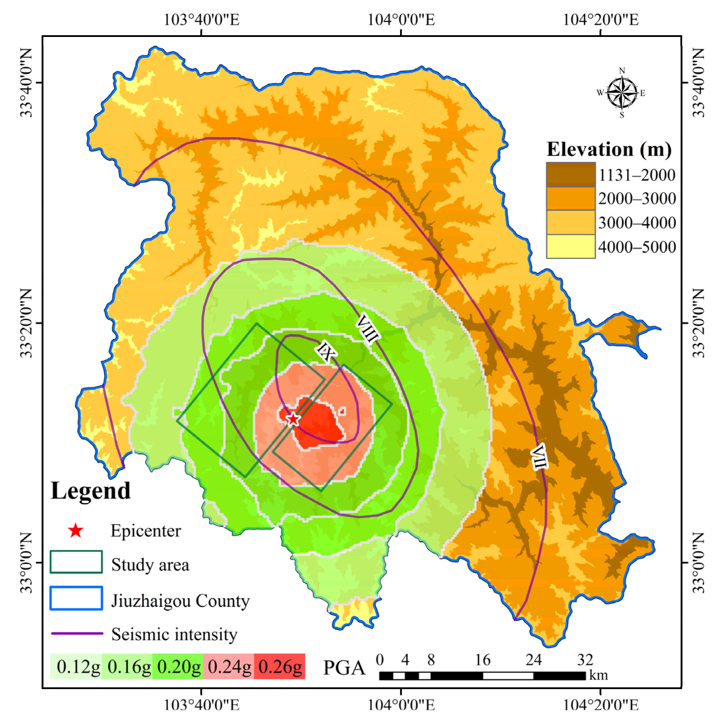
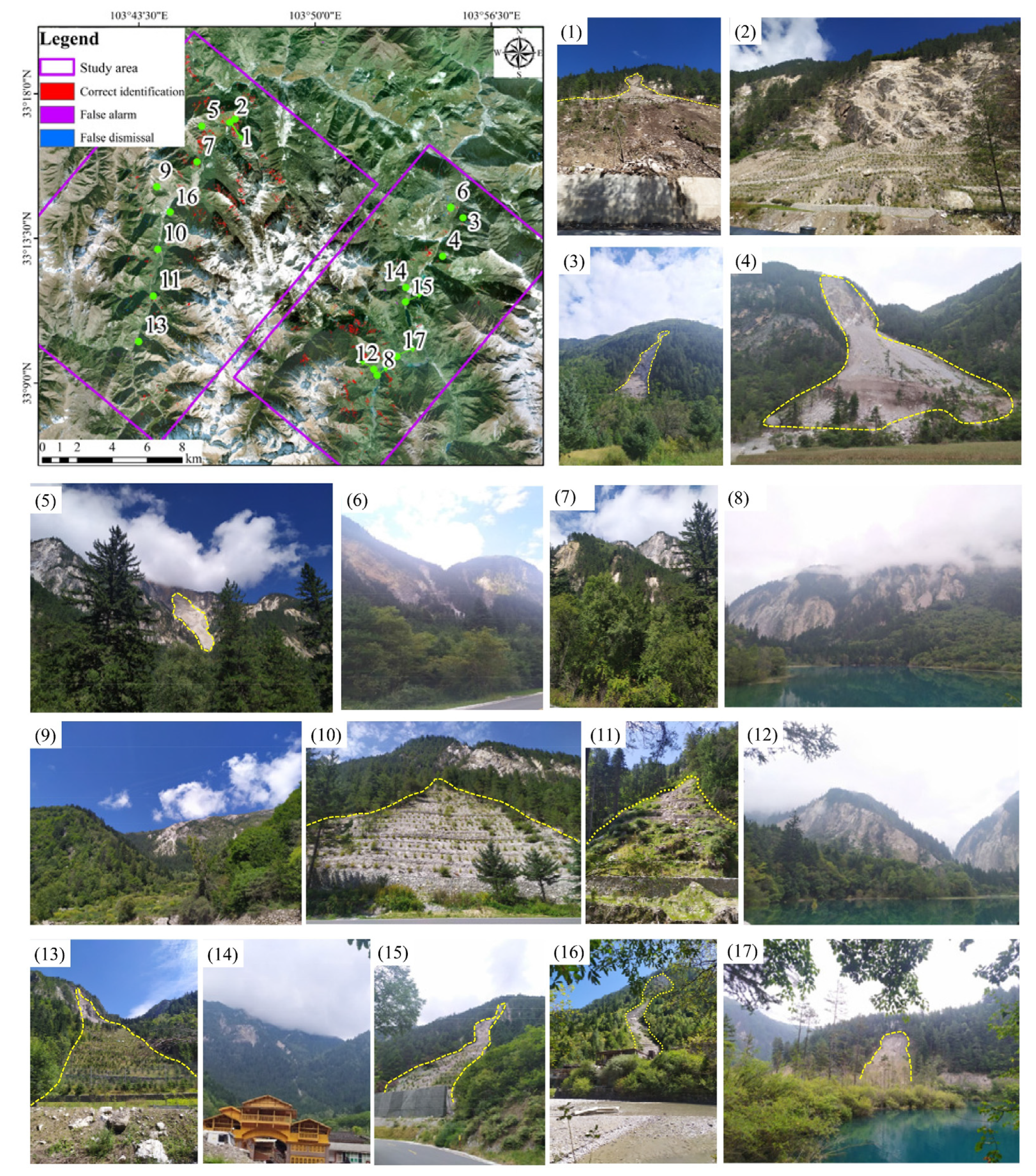
2. Study Area and Multisource Data

At 21:19:46 local time on 8 August 2017, a Ms 7.0 earthquake struck Jiuzhaigou County, Sichuan Province, China, with a focal depth of 20 km [31]. The epicenter was located at 33.20°N 103.82°E, and the peak ground acceleration (PGA) at the epicenter reached 0.26 g.
The earthquake affected 205,000 people, including 25 deaths, 525 casualties, and 6 missing people. A total of 73,671 houses were damaged to varying degrees [8,32,33].
The earthquake triggered 5563 landslides that covered an area larger than 9.45 km2 and were densely distributed within two regions [34], i.e., northwest and southeast of the epicenter. The size of these coseismic landslides is relatively small, and 92.31% of the coseismic landslides possess an area smaller than 1104 m2 (about 11 pixels) [35]. Moreover, the surrounding environments of the landslides were various, and coseismic landslides occurred in woodland or bare land, on roadsides, or by rivers. Therefore, coseismic landslide recognition after the Jiuzhaigou earthquake is a small-target recognition problem under various and complex environments. It is a difficult problem in the area of target recognition.
The study area Is located in the meizoseismal region, with an area of 435.63 km2. It stretches across the regions with seismic intensities of VII, VIII, and IX, and includes the above-mentioned two areas with densely distributed landslides (Figure 1). Moreover, the study area features intensive neotectonic movement, complicated active fault structures, alpine canyon landforms, steep topography, developed river systems, and a humid plateau climate.
Five types of multi-source data (Table 1) were employed to establish the recognition indices of coseismic landslides. (1) After processed by the L2A procedure, the pre-earthquake and post-earthquake Sentinel-2 Level 1C images were used to construct the spectral indices and NDVI that reflected the land cover change and vegetation damage during the earthquake. (2) Seismic data were used to establish the indices of PGA and distance to the seismogenic fault. (3) A geological map was adopted to build the stratum indice. (4) DEM was utilized to establish the topographic indices of elevation, slope degree, slope aspect, and mean curvature. (5) Meteorological data were used to construct the cumulative rainfall indice that reflected the effect of pre-earthquake precipitation.

3. Methods

The technology flow chart is shown in Figure 2, and includes three steps.
(1)
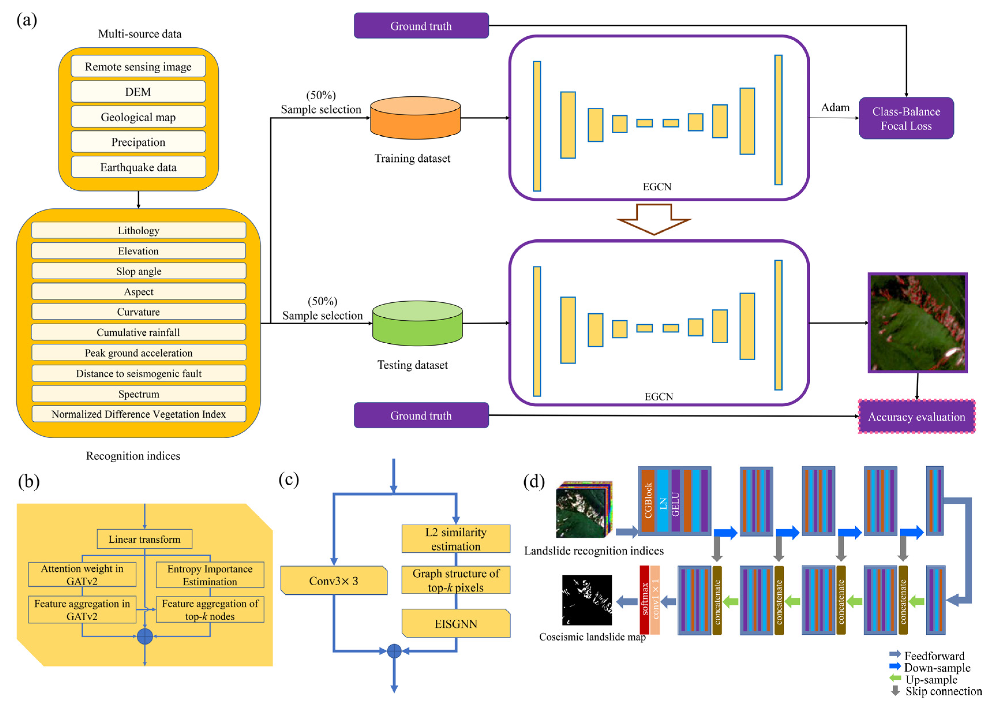
Establishment of recognition indices. The landslide identification indices are established according to the causal mechanism of the coseismic landslides and to the change in surface cover triggered by the coseismic landslides. These indices consist of the geological, topographic, environmental, meteorological, seismic, and spectral characteristics extracted from multi-source data.
(2)
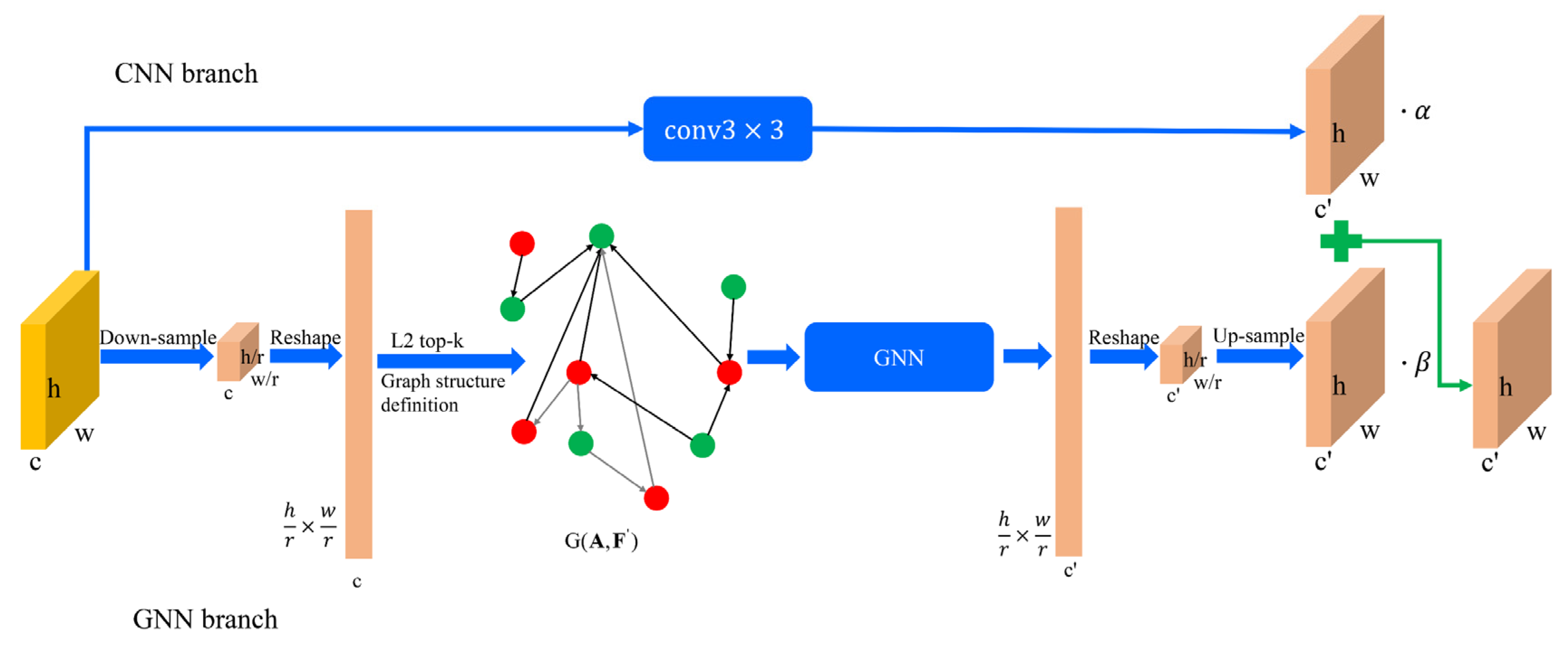
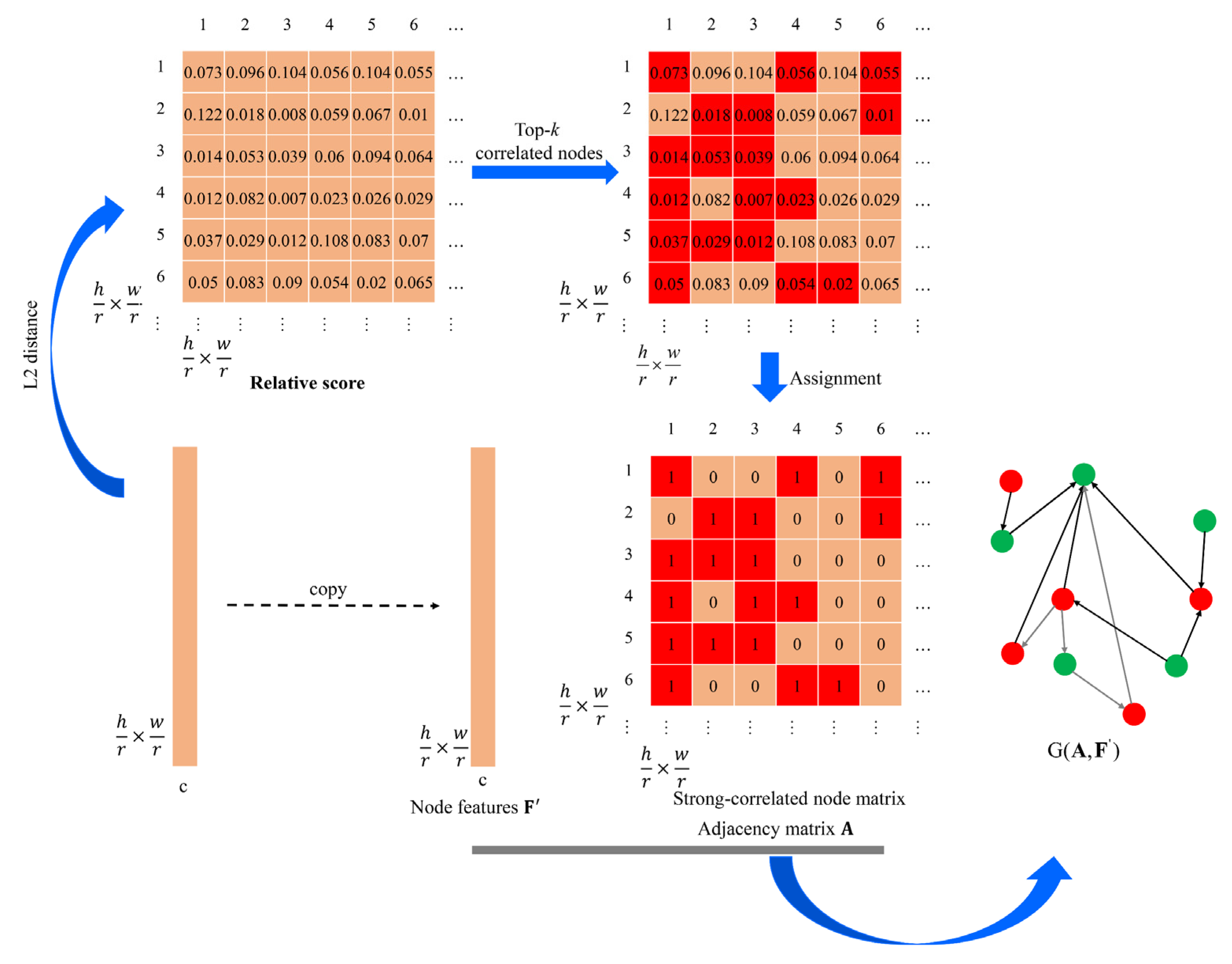
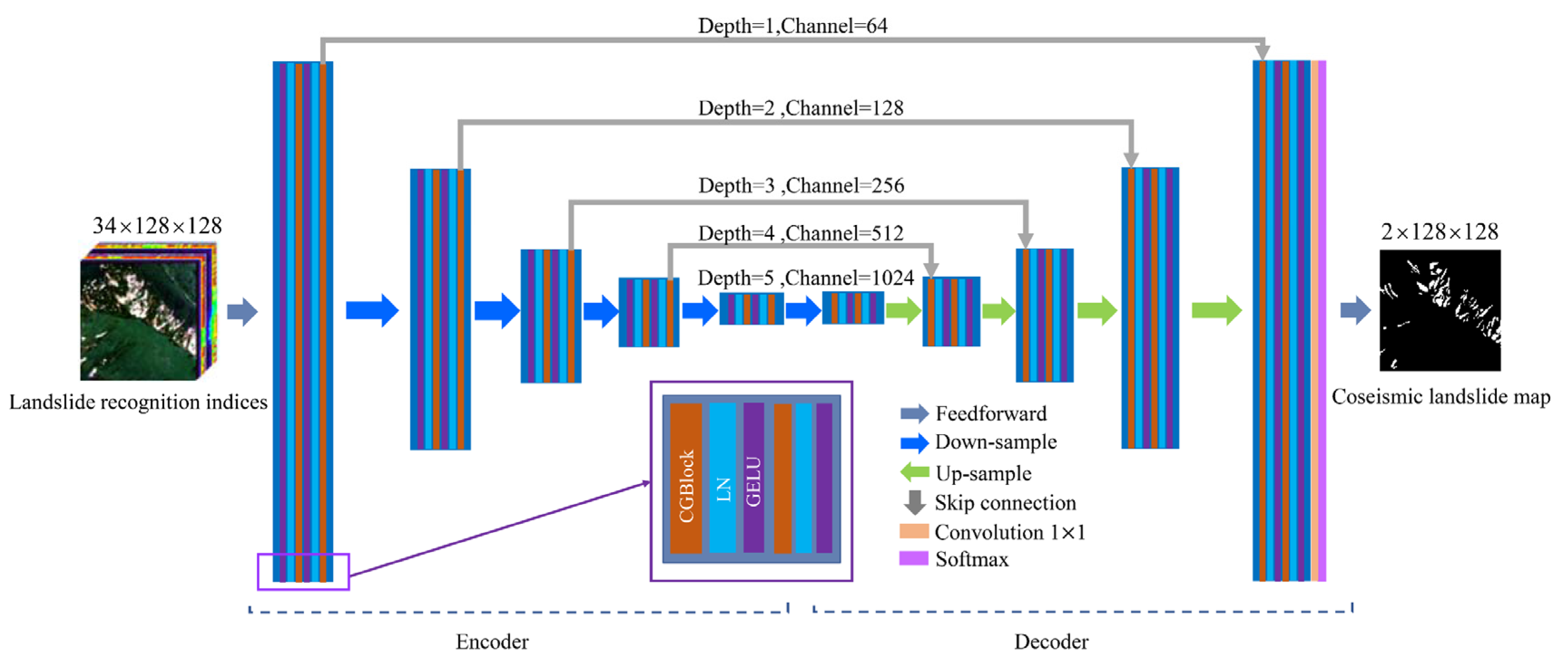
Construction of the landslide identification network EGCN. It is composed of 3 steps. (a) Design of a graph neural network, EISGNN. A selective aggregation graph neural network, EISGNN, is proposed based on GATv2, entropy importance coefficients, and a selective aggregation strategy of node features. The EISGNN can aggregate effective features and eliminate the influence of invalid context dependency. (b) Construction of a basic block CGBlock. A GNN branch including EISGNN is established to extract the global context dependency relationship. A CNN branch is established to extract the local spatial features. Thus, CGBlock is constructed by integrating the GNN and CNN branches via adaptive weights and an ACmix fusion mechanism. (c) Establishment of the deep network, EGCN. The EGCN employs CGBlock as the basic module and adopts an encoder–decoder structure to effectively integrate the low-level high-resolution features and high-level low-resolution features. Thus, the high-level high-resolution semantic features can be generated, and the high-level context relationship, low-level context dependency, and local spatial features can be effectively fused to improve the identification accuracy.
(3)
Automatic recognition of coseismic landslides. The established recognition indices are inputted into the EGCN to obtain the distribution of coseismic landslides. Note that EGCN is the overall network for coseismic landslide recognition. CGBlock is a basic module involved in EGCN and includes two branches of CNN and GNN, and EISGNN is the main part of the GNN branch in CGBlock.

3.1. Establishment of Landslide Recognition Indices

The established indices (Table 2) include three categories: landslide-controlling geoenvironment, landslide-inducing features, and surface cover change. These indices cover the timeline through pre-earthquake, earthquake, and post-earthquake. (1) The geoenvironmental indices control the occurrence and distribution of coseismic landslides and include the lithology, elevation, slope angle, slope aspect, and average curvature. The stratum indice is quantified according to the stratum age. Soft rocks or soft–hard interbedding rocks result in the development of unstable slopes that easily evolve into landslides during an earthquake. Moreover, high and steep mountainsides and mountaintops are conducive to coseismic landslide occurrence [37]. Considering its direction, the slope aspect is classified according to the angular ranges of directions on the polar coordinate. (2) The disaster-inducing factors trigger landslide occurrence and development, and consist of pre-earthquake precipitation and earthquakes. Thus, the disaster-triggering indices are composed of the pre-earthquake cumulative rainfall, PGA, and distance to the seismogenic fault. The cumulative rainfall indice is obtained by the Kriging interpolation method based on the precipitation station report. Rainwater scours and erodes slope surfaces and causes water and soil loss, and gully development. In addition, rainwater penetrates cracks, and immerses and softens rock and soil masses. Then, weak sliding surfaces form, and slopes become unstable and move. These creeping slopes tend to slide under an earthquake event. Therefore, an area with concentrated rainfall before an earthquake is generally a region with intensive coseismic landslides. In addition, PGA reflects the vibration strength of the ground’s surface, and thus controls the distribution of coseismic landslides. To make the PGA indice more beneficial for landslide recognition, it is quantified according to its value distribution. Furthermore, seismogenic faults lead to fragmented rock masses, and coseismic landslides are densely distributed near seismogenic faults. Thus, the distance to the seismogenic fault is graded according to the landslide’s distribution characteristics around it. (3) The surface cover variation indices are composed of the pre-earthquake and post-earthquake spectral indices stacked in the band dimension and the NDVI before and after an earthquake. The occurrence of coseismic landslides generally causes a change in the image spectral characteristics and the damage to vegetation coverage. As the spectral indices stacked in the band dimension and the NDVI difference index before and after an earthquake can reflect the surface cover change, they are regarded as surface cover change indices strongly correlated with the occurrence of landslides.

3.2. EISGNN Algorithm

At present, global context dependency is modeled by a spatial attention mechanism, which is usually computationally massive and generates a large amount of redundant context dependency relationships. The proposed EISGNN adopts a selective aggregation strategy in graphs to model effective context dependency in a global image. It can avoid the huge computation amount and reduce the false alarms caused by redundant context dependency relationships. In the EISGNN, Pixel i becomes Node i in a graph, and the recognition indices of Pixel i are the features of Node i. An entropy importance coefficient is defined by information entropy and cosine similarity to evaluate the information effectiveness of neighbor Node j to target Node i. The neighbor nodes corresponding to the top-k entropy importance coefficients are selected to produce effective context dependency from the extracted node features based on the GATv2 graph neural network [38].
The node representation process in the network of EISGNN is shown in Equation (1).
F = λ eisAggre ( G ( A , F ) ; θ e ) + μ F + W 1 F
where F indicates the input features, and F means the node features output from the GATv2 network. G ( A , F ) represents a graph composed of the node feature matrix F and the node adjacency matrix A .   θ e indicates the learnable weight for selective aggregation by entropy importance coefficients, and eisAggre(·) represents the node feature aggregation process according to the entropy importance-based selection strategy. W1 indicates a single-layer feedforward network. λ and μ are the hyperparameters that integrate the node features obtained by selective aggregation and the node features obtained by GATv2. The node representation process in EISGNN contains two steps: (1) attention-based feature aggregation in GATv2 and (2) selective feature aggregation based on the entropy-important coefficients (Figure 2b).

3.2.1. Attention-Based Feature Aggregation in GATv2

The node representation procedure in GATv2 is shown in Equation (2).
F = GATv 2 ( G ( A , F ) ; θ g ) = attenAggre ( m ( G ( A , F ) ) )
where θ g represents the learnable parameters in the GATv2 network. attenAggre(·) indicates feature aggregation based on attention weights (called attention aggregation). m(·) represents a feature mapping operation. The feature mapping process before attention aggregation is shown in Equation (3).
m ( ) = H = W 1 F ; H = { h 0 , h 1 h n } ; n = len ( H )
where h n represents the n-th node features, and the input node features are mapped to the updated node features. Attention aggregation indicates the feature sum of neighbor nodes weighted by attention scores (Equation (4)). N i represents the neighbor node set of Node i. Strong node features in a graph structure are obtained according to the weighted sum of neighbor node features.
attenAggre ( ) = j N i a i , j h j
where a i , j indicates the attention score. It is calculated using the learnable weight vector α after the concatenated features of target Node i and neighbor Node j are linearly transformed (Equation (5)).
a i , j = LeakyRELU ( α W 2 ( | | ( h i , h j ) ) )
where | | represents the concatenation operation of node features. LeakyRELU(·) indicates the LeakyRELU activation layer. To make the feature aggregation process of neighbor nodes more stable, the Softmax function is used to normalize the attention coefficients (Equation (6)).
a i , j = softmax j ( a i , j ) = exp ( a i , j ) k N i exp ( a i , k )

3.2.2. Selective Feature Aggregation Based on Entropy-Important Coefficients

The node features obtained from GATv2 attention aggregation have some redundant information from heterogeneous nodes. In order to alleviate the influence of heterogeneous neighbor nodes on the representation of the target node, an entropy importance selection strategy is suggested to reinforce the effective features from homogeneous neighbors and to reduce the influence of invalid features from heterogeneous neighbor nodes. Selective aggregation based on the top-k entropy importance coefficients has three steps: (a) determination of entropy importance coefficients, (b) selection of the neighbor node set, and (c) node feature aggregation.
(a) Determination of entropy importance coefficients
Information entropy and cosine similarity are used to determine the entropy importance coefficients and to evaluate the effectiveness of the features of neighbor Node j to target Node i. An entropy importance coefficient is defined in Equation (7).
e i c i , j = 1 e i , j + s i , j ;   e i , j = h i log h j ;   s i , j = h i h j h i h j
where e i , j indicates information entropy and s i , j represents cosine similarity. The inverse of information entropy ensures that the larger the value of an entropy importance coefficient, the more effective the information that the corresponding neighbor Node j contributes to target Node i. The linear transformation of input features is performed in Equation (8) before the entropy importance coefficients are calculated. W 3 indicates a single-layer feedforward network.
H = W 3 F ; H = { h 0 , h 1 h n } ; n = len ( H )
To ensure the stability of the selective aggregation process, the entropy importance coefficients are also normalized before the weighted sum of node features is calculated.
(b) Selection of neighbor nodes
The neighbor nodes of Node i are sorted in a descending order according to the values of the entropy importance coefficients. Then, the neighbor nodes corresponding to the top-k entropy importance coefficients are selected to conduct later feature aggregation. The selection procedure of the neighbor node set is shown in Equation (9).
s e l e c t i n d e x i = i n d e x i [   : k ] ; i n d e x i = argsort i ( e i c i , j )
where argsort(·) is a sorting function. It sorts the neighbor nodes of Node i according to the values of entropy importance coefficients to obtain the indices i n d e x i of the sorted neighbor nodes. s e l e c t i n d e x i indicates the neighbor nodes of Node i corresponding to the top-k entropy importance coefficients. Actually, the number of selected neighbor nodes for a target node i varies. Given the universality of EISGNN, the choice proportion select_factor is defined to dynamically adjust the parameter k, i.e., k = int ( N i *select_factor). N i is the number of neighbor nodes and k reflects the number of selected neighbor nodes. The value setting of select_factor is shown in Section 4.1, and the influence of different select_factor values on network performance is discussed in Section 4.4.4.
(c) Node feature aggregation
Feature aggregation is conducted from the selected neighbor nodes to the target node, and the feature aggregation procedure is shown in Equation (10).
eisAggre ( ) = s s e l e c t i n d e x i e i c i , s F s
where F s indicates the features of the selected neighbor nodes after GATv2 attention aggregation. e i c i , s indicates the entropy importance coefficient between Node i and its selected neighbor nodes. s e l e c t   i n d e x i represents the set of selected neighbor nodes.
Similar to Transformer, the suggested EISGNN can perform node representation in a multi-head formation. For the multi-head EISGNN, the final output node features are shown in Equation (11):
F = c = 1 C λ c eisAggre ( G ( A , F , c ) ; θ e c ) + μ c F , c + W 1 c F
where | | represents the concatenation operation of node features. C indicates the parallel number of GATv2 attention aggregation and entropy importance-based selective aggregation.

3.3. CGBlock

CGBlock is composed of a CNN branch and a GNN branch (Figure 3). The CNN and GNN branches extract local spatial features and global context features, respectively. The global context features are relatively stable and independent of environmental backgrounds, and are extracted by feature aggregation among the strongly correlated nodes in a GNN branch. The local features reflect landslide-varying detail features (unstable features) under different environments and are acquired by a CNN branch. The relatively stable global context dependency features and the unstable local features are integrated to generate the relatively stable identifiable characteristics of landslides by adaptive weights (the learnable weights-weighted feature fusion mechanism for ACmix [30]). As a result, the environmental adaptability can be improved.
The CNN branch adopts a convolutional layer with a kernel size of 3 × 3, and the GNN branch includes a down-sampling layer, an up-sampling layer, a graph definition layer, and a GNN module. The GNN module (i.e., EISGNN) takes each image pixel as a node; thus, it can extract contextual features among various pixels. The down-sampling layer employs a nearest-neighbor interpolation method to reduce the spatial size of feature maps and to decrease the computational amount.
The graph definition layer determines the selected top-k pixels according to the L2 distance between one pixel and other pixels as the context structure of the pixel (Figure 4). The L2 relative score of features between one pixel and other pixels is calculated as Equation (12).
r e l a t i v e s c o r e = L 2 ( reshape ( F ) )
where reshape(·) is the reshaping operation that converts the feature map F c , h / r , w / r into F h w / r 2 , c .   r e l a t i v e s c o r e ( 0 + ) h w / r 2 , h w / r 2 indicates the distance matrix among pixels. For target Pixel i and another Pixel j, a smaller relative score between Pixel i and Pixel j indicates that Pixel j is closer to Pixel i, and that Pixel j is more similar to or strongly correlated with Pixel i. h and w indicate the height and width of the input feature map. r indicates the down-sampling factor. For any pixel i, the top-k pixels strongly correlated to pixel i are selected as the context structure of pixel i in terms of the value of r e l a t i v e s c o r e i .
Therefore, during node representation in the GNN module, the valid features from strongly correlated pixels can be effectively utilized and the interference information from weakly correlated pixels can be reduced in feature aggregation. The adjacency matrix A among all pixels is initialized by a zero matrix. For any pixel i, the pixels corresponding to the top-k L2 distances are considered to have adjacency relationships with pixel i (Equation (13)).
A [ i n d i c e [ i , : k ] ] = 1 ; i n d i c e = argsort ( r e l a t i v e s c o r e )
where argsort(·) computes the corresponding pixel indice after the variable relative score is arranged in an ascending order. indice[i,:k] represents the indices of the top-k pixels similar to Pixel i, and these pixels constitute the receptive field of Pixel i. In the CNN branch, the receptive field of convolutional operation is a local and regular rectangle range; thus, local spatial features can be extracted. Different from the CNN branch, the receptive field of the GNN branch is global and irregular; thus, effective global context features can be extracted. The value setting of k is shown in Section 4.1, and the effect of different k values on network performance is discussed in Section 4.4.3. Once the interpixel adjacency matrix A and the node feature matrix F are obtained, graph G ( A , F ) with context structures can be constructed. Note the contextual features obtained by the EISGNN module are up-sampled to the same scale of the local spatial features in the CNN branch by a deconvolution layer (the up-sampling function in Figure 3). This guarantees that the local spatial features from the CNN branch and the context features from the GNN branch have the same spatial structure when they are fused by learnable hyperparameters α and β.

3.4. EGCN

EGCN is a landslide recognition framework with an encoder–decoder structure (U-Net as the baseline). It is a semantic segmentation model and fuses low-level high-resolution semantic information and high-level low-resolution semantic information to produce high-level high-resolution semantic features. Therefore, it can better depict the shape and boundary characteristics of small landslides. EGCN uses CGBlock as the basic module (Figure 5) and mainly includes the CGBlock layers, LN (Layer Normal) layers, GELU (Gaussian Error Linear Units) activation layers, pooling layers, deconvolution layers, and concatenation layers. X and Y are the input and output of EGCN, respectively, and EGCN is defined as Equation (14).
Y = EGCN ( X ) = Decoder ( Encoder ( X ) )
where X c , h , w ,   and   Y n c l a s s , h , w . c indicates the number of channels in the input samples, and nclass represents the target category number. The input feature encoding process is shown in Equations (15)–(18), and the feature decoding process is shown in Equations (19)–(21).
Similar to U-Net [39], at each depth in the encoder or decoder, two CGBlock layers are used to extract local spatial features and context dependency relationships. Each CGBlock is followed by an LN layer and a GELU activation layer, so the feature-extraction process by the first CGBlock is shown in Equation (15).
F 1 , 1 = GELU ( LN ( CGBlock 1 , 1 ( F 1 , 0 ) ) ) F 1 , 0 = X
where CGBlock 1 , 1 indicates the first CGBlock layer at the 1-st depth in the encoder and F 1 , 0 represents the input features at the 1-th depth. F 1 , 1 represents the local spatial and contextual fusion features at the 1-th depth extracted from input feature F 1 , 0 . Then, the output features at the 1-th depth are as follows (Equation (16)):
F 1 , 2 = f 1 , 2 ( f 1 , 1 ( F 1 , 0 ) )
where f 1 , 1 indicates the function consisting of CGBlock 1 , 1 , an LN layer, and a GELU layer. f 1 , 2 indicates the function consisting of CGBlock 1 , 2 , an LN layer, and a GELU layer. F 1 , 2 represents the output features at the 1-th depth of the encoder. In order to reduce the computation effort, when the higher-level features are extracted, every two CGBlock layers are followed by a pooling layer (the down-sampling function in Figure 5) (Equation (17)).
F 2 , 0 = pool ( F 1 , 2 )
where pool(·) represents the maximum pooling operation with a kernel size of 2 × 2. Then, the output features at the d-th depth in the encoder can be defined as follows (Equation (18)):
F d , 2 = f d , 2 ( f d , 1 ( F d , 0 ) ) ; F d , 0 = pool ( F d 1 , 2 )
where d ∈ [2, 5]. In particular, the depths in both the encoder and decoder are 5, and the 5-th depth has only one CGBlock. Following U-Net, the numbers of features from the 1-st depth to the 5-th depth in the encoder or decoder are 64, 128, 256, 512, and 1024, respectively. The down-sampling factors r in a CGBlock are 16, 8, 4, 2, and 1, respectively. After a series of hierarchical features are extracted, the features in different layers are fused and transformed in the decoder. At the 5-th depth, there is no higher-level feature to merge with; thus, at this depth, CGBlock is only used for transformation operations (Equation (19)).
F 5 , 2 D = f 5 , 1 D ( F 5 , 1 ) = GELU ( LN ( CGBlock 5 , 1 D ( F 5 , 1 ) ) )
in which f 5 , 1 D indicates the first function at the 5-th depth in the decoder, consisting of CGBlock 5 , 1 D , LN, and GELU. At the other depths in the decoder, the lower-level features output from the d-th depth in the encoder will be fused with the higher-level features input to the d-th depth in the decoder. Before fusion, higher-level input features in the decoder need to be up-sampled to the same resolution as the lower-level features output from the d-th depth in the encoder (Equation (20)).
F d , 0 D = upconv ( F d + 1 , 2 D )
where d ∈ [1, 4] and upconv(·) indicates the deconvolution layer with a kernel size of 2 × 2. Therefore, the output feature at the d-th depth in the decoder is shown in Equation (21).
F d , 2 D = f d , 2 D ( f d , 1 D ( | | ( F d , 0 D , F d , 2 ) ) )
where | | represents a concatenation operation. After the second CGBlock layer at the 1-st depth in the decoder, features are mapped to the probability belonging to each category by a convolution layer with a kernel size of 1 × 1 and by a softmax layer (Equation (22)).
Y = softmax ( conv 1 × 1 ( F 1 , 2 D ) )

3.5. Loss in Landslide Recognition

Compared with non-landslide samples, landslide samples have much smaller areas and are fewer in quantity. Thus, coseismic landslide recognition is a class imbalance problem. Given this problem, a learning weight is used to balance the sample numbers of different classes. Focal Loss [40] is employed to increase the learning weight values for difficultly recognized samples. Therefore, Focal Loss with balanced weight values is employed as the loss function for coseismic landslide recognition.
For the class imbalance problem, the current approach generally refines the cross-entropy loss function and adopts the reciprocal of the number ratio of each class of samples in the groundtruth to weight the predicted probabilities of the class (Equation (23)).
= n h w c n c l a s s w c y n , c log y n , c ; w c = h w n h w int ( y n , c = = 1 )
where y n , c [ 0 , 1 ] indicates the predicted probability that Sample n belongs to Class c. y n , c { 0 , 1 } indicates the groundtruth of Sample n. w c represents the class-balanced weight of Class c, i.e., the reciprocal of the number ratio of Class c samples in the groundtruth. This class-balanced weight is sensitive to the learning rate value, requires a large number of iterations, and easily causes overfitting. To solve the difficulty in class-balanced weights during network training, the balanced weight based on effective sample sizes [41] is adopted in the loss function (Equation (24)).
w c = 1 η 1 η n u m c ; n u m c = n h w int ( y n , c = = c )
where η indicates the hyperparameter controlling the ratio of effective samples (pixels). n u m c indicates the number of pixels that belong to Class c in the groundtruth. In order to reduce the learning difficulty in misidentified targets, Focal Loss is employed, and a learning weight is added to the misidentified pixels according to the negative number of recognition probability (Equation (25)). Thus, the network can better learn the features of the misidentified targets.
f o c a l = n h w c n c l a s s ( 1 y n , c ) γ log ( y n , c )
in which γ indicates the factor that controls the amplification scale of learning weights. Therefore, the loss function for landslide recognition is defined as Equation (26).
c b f o c a l = n h w c n c l a s s w c ( 1 y n , c ) γ log ( y n , c )

4. Results and Discussion

4.1. Algorithm Parameters and Datasets

4.1.1. Algorithm Parameters

The value setting of the network parameters in the EGCN is shown in Table 3. The initial values of λ and μ are both 1.0. This makes the initial fusion of node representations obtained from attention aggregation and from selective aggregation more stable. Referring to the value setting in ACmix, the initial values of α and β were both set to 1.0. This ensures that the local spatial features and context features are equally fused, so the initial landslide recognition performance of the EGCN is relatively good.
Regarding the spatial structure in the CNN branch, the convolutional layer with a kernel size of 3 × 3 possessed a receptive field of eight neighbors; thus, k was set to 8. It could decrease the amounts of redundant context structures and computational complexity. Similar to the Swin Transformer, the value of head C in the multi-head EISGNN was set to 8. In addition, select_factor in selective aggregation controlled the number of selected neighbor nodes and was set to 0.8. This ensured that most of the neighbor nodes could participate in feature aggregation and prevented the reduction in network performance due to the sharp decrease in the number of nodes participating in aggregation.
The Adam optimizer was applied to iteratively train the network based on the Poly strategy. According to Deeplab V3 [42], the initial learning rate was set to 0.0001, and the weight decay was set to 0.0007 [11]. Moreover, the values of the loss parameters of η and γ were the same as those in Cui et al. [41].

4.1.2. Selection of Training and Testing Sets

The collected multi-source data in Section 2 were used to establish recognition indices. The established recognition indices in Section 3.1 were stacked in the band dimension and formed a large raster data set combined with landslide inventory. To train and evaluate the model, the samples from the raster dataset were randomly split into training and testing samples. The selection process of training and testing samples was composed of three steps.
(a) Region clipping. The raster data set of the whole study area was clipped into samples with a size of 128 × 128 from the bottom-left to the top-right by a sliding window with a stride of 96, and they were numbered from 0.
(b) Sample selection. To alleviate the impact of class imbalance on landslide recognition, the degree of imbalance in the numerical proportions of landslide pixels and background pixels needed to be decreased. The samples from the background category and the samples with very low proportions of landslide pixels were both discarded after region clipping. In this work, the sample selection process is shown in Equation (27).
P r i = N i + N i + + N i ; s e l e c t s a m p l e s = where ( P r > s e l e c t r a t i o )
where P r i indicates the proportion of landslide pixels in the ith sample, and N i + and N i indicate the numbers of landslide pixels and non-landslide pixels in the ith sample, respectively. selectsamples represents the indices of the selected samples. The function where(·) computes the index of elements conforming to a special condition. As the proportions of landslide pixels in samples mostly fell between 0 and 0.02, selectratio took a medium value of 0.01. Thus, among the 1085 samples in the study area, 1040 samples remained after sample selection.
(c) Establishment of training and testing samples. After sample selection, about half of the total randomly shuffled samples were selected as the training set, and the remaining samples were taken as the testing set. It is worth noting that samples with some overlapping regions were added to the same sample sets when selected. Finally, the number ratios of landslide to non-landslide pixels in the training dataset (522 samples) and testing dataset (518 samples) were 1:27 and 1:29, respectively.

4.1.3. Evaluation Criteria of Landslide Recognition

All quantitative criteria for the experiments are shown in Table 4. As OA and mIOU evaluated the identification accuracy of all categories equally, they could not reflect the recognition balance degree of various categories. Therefore, they could not evaluate the landslide recognition results very well for those samples with a very small proportion of landslide pixels. F1, Kappa, Precision, and Recall could comprehensively evaluate the accuracy of each category and also reflect the degree of balance of each category’s accuracy well. The Kappa coefficient could evaluate the consistency of the number of each category in the prediction results and labels. It was more sensitive to the small difference between the predicted landslide distribution and the real landslide distribution; thus, it could well-evaluate the landslide recognition results. In particular, Params was also applied to evaluate the performance of models. As a static evaluation criterion, Params could help to measure the model parameter size.

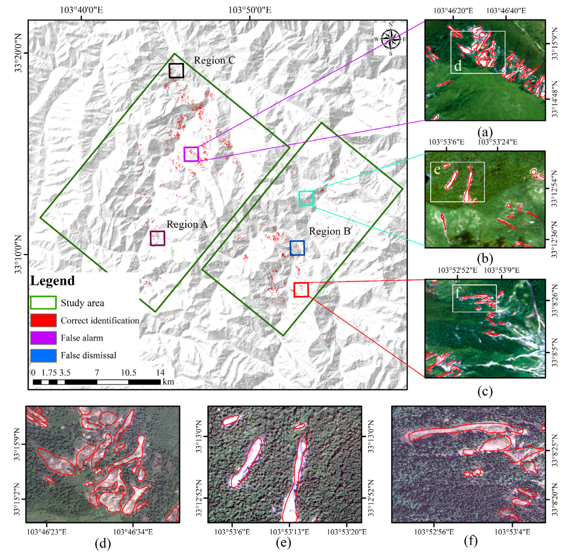
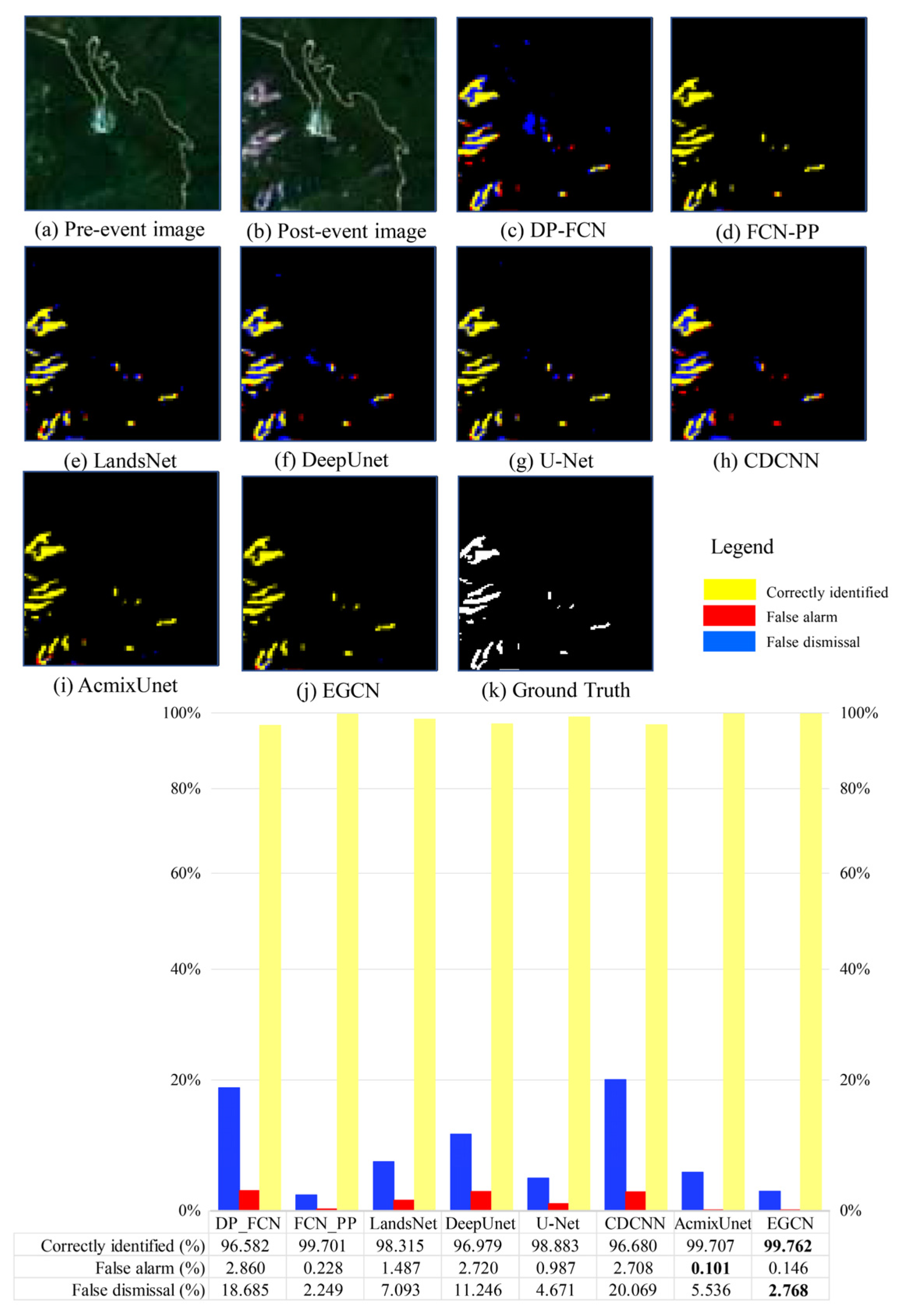
4.2. Recognition Results of Coseismic Landslides

To illuminate the superiority of the proposed EGCN, it was compared with other state-of-the-art landslide recognition methods, including change detection-based methods and semantic segmentation-based methods. The change detection-based methods for landslide recognition consist of DP-FCN [2] and CDCNN [11]. The semantic segmentation-based methods for landslide identification include DeepUnet [15], FCN-PP [17], LandsNet [18], AcmixUnet, and U-Net [39]. The parameter values in DP-FCN, DeepUnet, CDCNN, LandsNet, and FCN-PP were the same as the ones in the original papers. ACmix [30] configures convolution and self-attention in a shared-parameter way. It extracts and adaptively merges local spatial features and semi-global context dependencies. AcmixUnet is a semantic segmentation network constructed following the U-Net structure, including ACmix layers, LN layers, GELU activation layers, pooling layers, and deconvolution layers.
The recognition result of coseismic landslides in the study area is shown in Figure 6. In order to highlight the advantages of the proposed method in various environments, three regions (Region A, Region B, and Region C in Figure 6) were selected as examples. The three regions were all test regions that were not employed to train the network. The identification results of the eight methods in the three regions are shown in Figure 7, Figure 8 and Figure 9.
The environmental characteristics and landslide sizes in the three regions are shown in Table 5. The EGCN outperformed the other seven methods and generally possessed the highest accuracy, the lowest false alarm rate, and the lowest false dismissal rate. Note that the environment in the study area mainly included woodland, grassland, bare land, rivers, and roads; thus, the three regions contained all the environmental types.
Furthermore, the field validation photos of the identified coseismic landslides are shown in Figure 10.

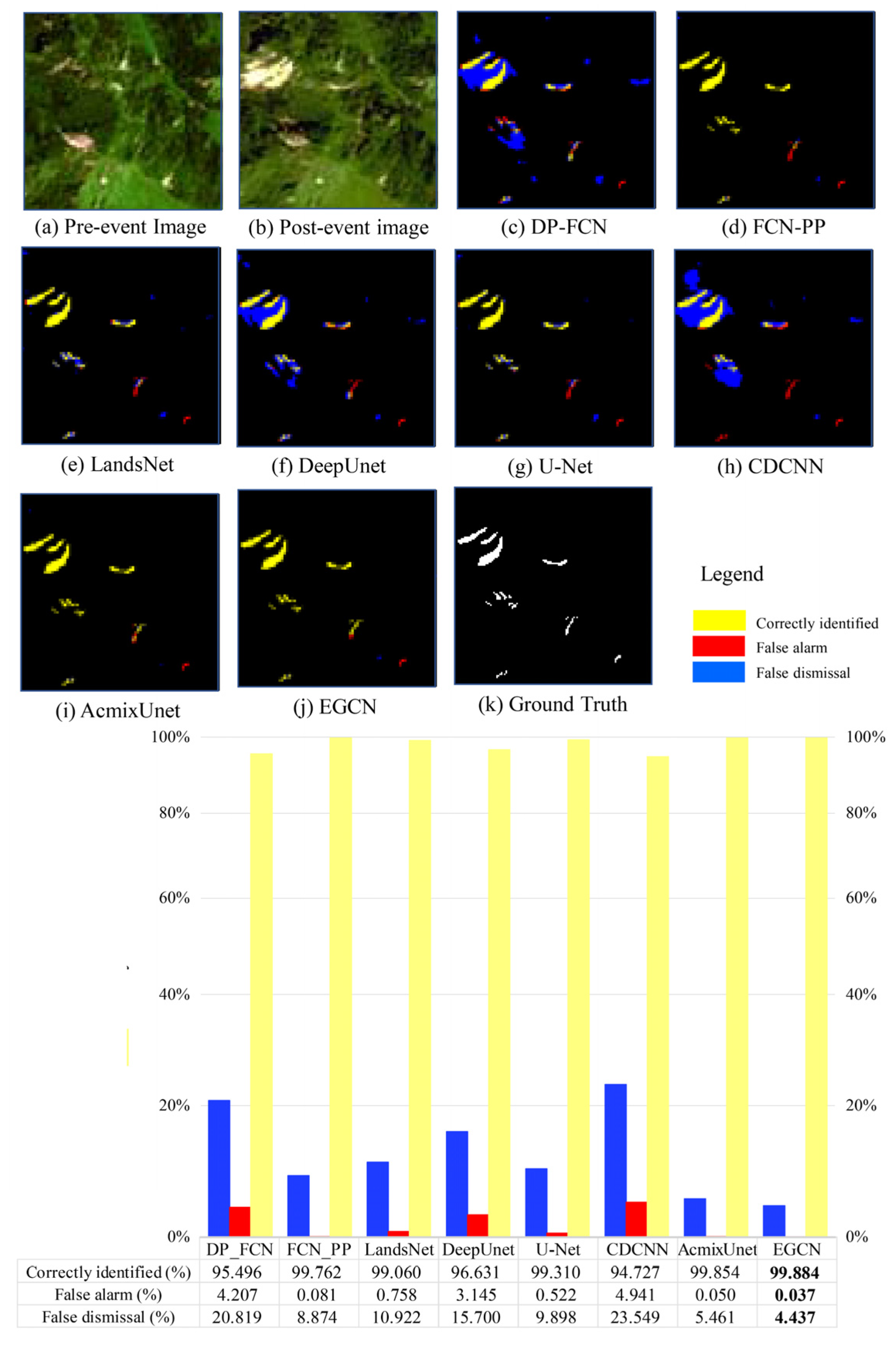
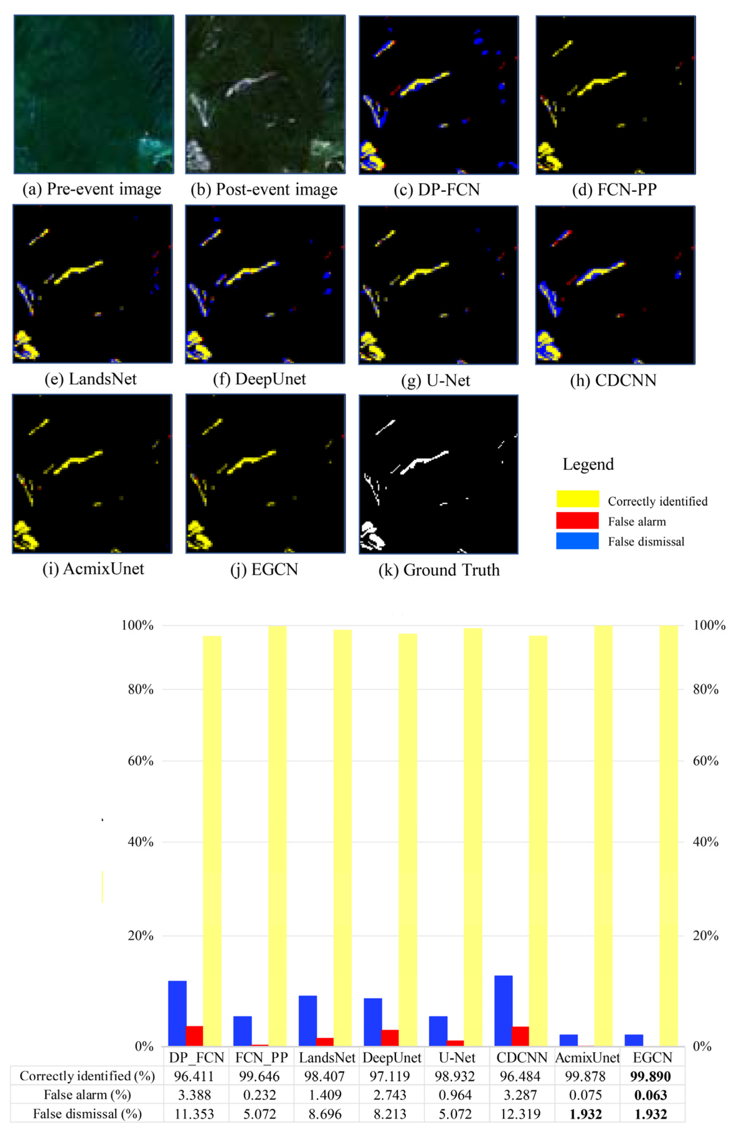
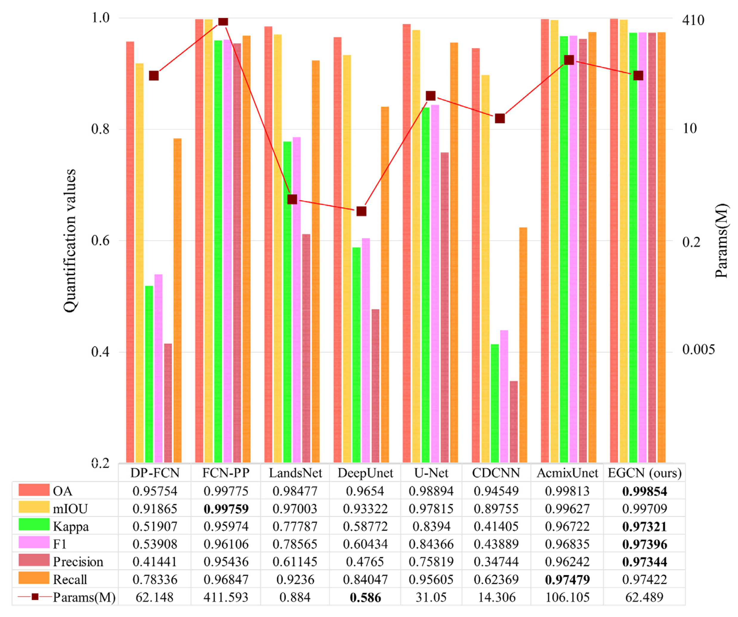
4.3. Precision Comparison of Various Algorithms

The precision evaluation of eight methods on the test set is shown in Figure 11. Among the seven methods for comparison, LandsNet, DeepUnet, and CDCNN had relatively higher OA and mIoU values and fewer parameters. However, they possessed relatively low values for Precision, Recall, F1-score, and Kappa. FCN-PP and AcmixUnet based on the semantic segmentation feature high performances in landslide recognition and had the highest mIoU and Recall values, respectively. However, they were both characterized by huge numbers of parameters. In other words, their higher mIoU and Recall values were at the cost of an increase in the number of parameters. U-Net maintained a moderate number of parameters and a medium landslide recognition performance.
Compared with the above seven methods, the proposed EGCN had the highest OA, Kappa, F1-score, and Precision values. Moreover, it had fewer parameters than AcmixUnet and FCN-PP. However, the feature extraction types of EGCN and AcmixUnet were similar (the only difference between EGCN and AcmixUnet was that EGCN used parameter-shared convolution to simulate Patch MSA to model semi-global context dependencies, while EGCN utilized EIGNN modules to model global context dependencies), and the OA and mIoU of AcmixUnet reached a relatively high level; however, the improvement space for EGCN was too small. As a result, EGCN and AcmixUnet seemed to be almost the same in terms of OA and mIoU, and the OA and mIoU of EGCN did not improve significantly. In contrast, the F1-score and Kappa coefficient of EGCN were significantly higher than those of AcmixUnet and the other six methods. This indicates that EGCN could identify various categories (landslides and backgrounds) in a more balanced and accurate manner with fewer model parameters. In summary, the suggested EGCN generally achieved the highest performance in landslide recognition.

4.4. Influence of Recognition Indice Set and Network Hyperparameters

Ablation experiments were conducted on the following four aspects: (1) different recognition indice sets, (2) different attention modules in the modeling of context dependency relationship (Figure 12b), (3) different pixel numbers in the construction of a graph (Figure 12c), and (4) different m values in the selective aggregation strategy (Figure 12d).
These ablation experiments could explore the influence of different recognition indice sets on landslide recognition and verify whether the context dependency modeled by EISGNN was more efficient than that modeled by the typical attention methods of MSA (Patch-based multi-head self-attention) and ESA. In addition, they could explore the ability of EISGNN to model context dependency from graphs of different complexities. Moreover, these experiments could analyze the influence of different numbers of neighbor nodes in feature aggregation on landslide recognition performance.

4.4.1. Do Different Recognition Indice Sets Affect the Results of Coseismic Landslide Recognition?

Recognition indice sets were applied to identify coseismic landslides, and the influence of different recognition indice sets on landslide recognition is shown in Table 6. Table 6 (a) indicates the recognition indice set composed of the spectral indices before and after an earthquake; (b) represents the recognition indice set characterized by the spectral indices before and after an earthquake and terrain indices (slope angle, slope aspect, and curvature); (c) indicates the recognition indice set characterized by the spectral indices before and after an earthquake, terrain indices (slope angle, slope aspect, and curvature), and environmental indices (NDVI); and (d) indicates the recognition indice set that considers the causal mechanism of coseismic landslides (details of the recognition indice set is introduced in Section 3.1).
Compared with (a), the experiment on (b) obtained higher OA, mIoU, Kappa, F1-score, and Precision values. This suggests that the addition of terrain indices and environmental indices increased the discrimination of extracted features. However, compared with the landslide recognition results of (a) and (c), the mIoU, Kappa, and F1-score of the experiment on (b) decreased significantly. This may suggest that terrain indices may not be used as independent recognition indices for coseismic landslides; only the interaction of terrain indices and other indices (environmental indices, etc.) can produce highly discriminative features.
Compared with (a), (b), and (c), the experiment on the recognition indice set that considered the causal mechanism of coseismic landslides obtained higher OA, mIoU, F1-score, and Kappa values. This indicates that the recognition indice set composed of spectral indices, geology indices, terrain indices, environment indices, and earthquake indices was more effective for coseismic landslide recognition.

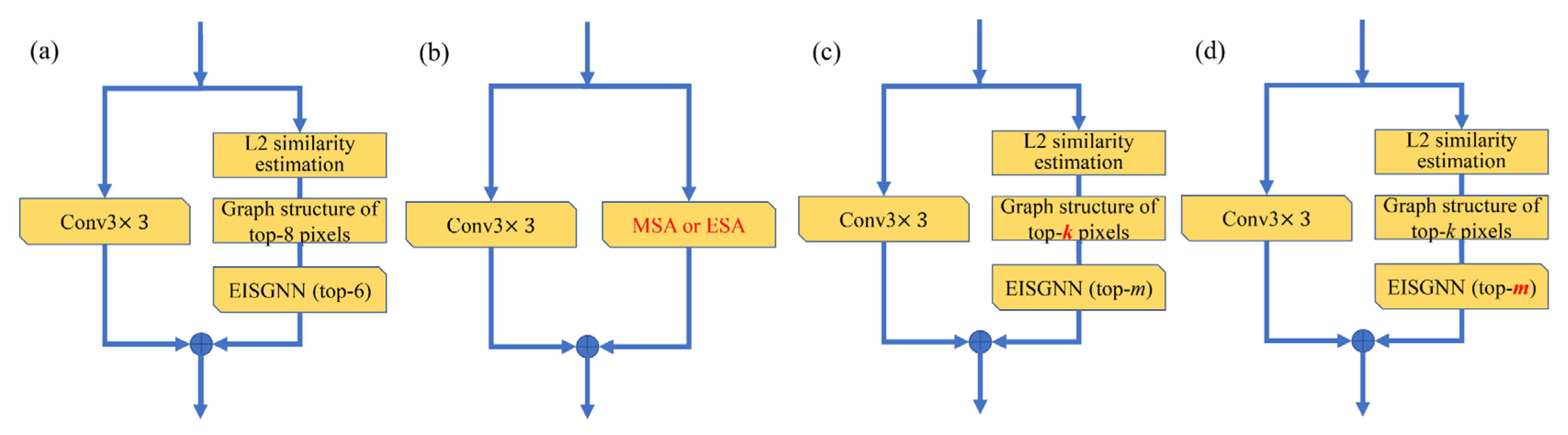
4.4.2. Is the GNN Branch More Efficient than Other Attention Modules of MSA and ESA?

Context dependency was modeled by an attention module, and the influence of different attention modules on the network performance is shown in Table 7 (b). The current popular attention modules of MSA and ESA were employed to conduct comparisons. MSA and ESA were the attention modules adopted in Swin Transformer and SegFormer, respectively.
When the GNN branch was replaced with other attention methods, it could still achieve high recognition accuracies. Thus, the fusion of attention-modeled context features and local spatial features was effective in landslide recognition. Moreover, the GNN branch outperformed the attention modules of MSA and ESA and possessed the highest accuracy.

4.4.3. Is EISGNN Adaptable to Graphs of Different Complexity?

The complexity of a graph is embodied as the number of nodes (pixels) constituting a graph. The influence of different node numbers on the network performance is shown in Table 7 (c).
The graph structure exhibited growing complexity when the node number k increased from 8 to 32. The recognition accuracy generally increased, accompanied by the increasing graph complexity, because more comprehensive and abundant context features were extracted from a more structure-complicated graph. Despite the variation in graph complexity, the identification accuracies all reached high levels; thus, EISGNN had a strong adaptability to changing graph complexity.

4.4.4. Does the Number of Neighbor Nodes in Feature Aggregation Influence the Network Performance?

The selection proportion select_factor controls the number (m) of neighbor nodes selected for feature aggregation, i.e., m = int(select_factor*k). The influence of different select_factor values on recognition accuracy is shown in Table 7 (d).
When the value of select_factor increased, the number of selected neighbor nodes correspondingly grew. Thus, the features from more useful nodes participated in aggregation, and the identification accuracy also increased. However, when all of the neighbor nodes joined in aggregation (select_factor = 1.0), the recognition accuracy decreased because the superfluous and invalid features were involved in aggregation. Thus, the best value of select_factor was 0.8.

5. Conclusions

Small landslides under various complicated environments are challenging to recognize. To solve this problem, EGCN is proposed to integrate the global and useful context features and local spatial characteristics at both high and low levels for coseismic landslide recognition. Its features and innovations are embodied as three aspects: (1) The recognition indices of EGCN are established according to the causal mechanism of coseismic landslides, guaranteeing the rationality of landslide identification. (2) The EISGNN module in the GNN branch is suggested to model global useful context dependency by feature aggregation among nodes with high entropy importance. The global context features are relatively stable, independent of environment backgrounds, and integrated with the local varying detail features (unstable features) extracted by the CNN branch to generate the relatively stable identifiable characteristics of landslides by adaptive weights. As a result, the environment’s adaptability can be improved. (3) Owing to the use of CGBlock as the basic module and U-Net as the baseline, EGCN fuses relatively stable identifiable low-level high-resolution characteristics and relatively stable identifiable high-level low-resolution characteristics to generate identifiable high-level high-resolution features. Therefore, the shape and boundary of small landslides can be better depicted and the identification accuracy of small targets can be improved.
The EGCN method achieved high accuracy in the meizoseismal region of the Ms 7.0 Jiuzhaigou earthquake and outperformed the popular deep learning methods of DP-FCN, FCN-PP, LandsNet, DeepUnet, U-Net, CDCNN, and AcmixUnet. In addition, EGCN could be not only used for coseismic landslide recognition, but also be applied to the recognition of other small targets. When the input data are the recognition indice set established by the multi-temporal spectral features before landslides and other auxiliary identification indices, EGCN can also be used to extract the minimal land changes that could be used as a predecessor to a landslide (the single minimal land change area should be greater than or equal to 800 m2) after the parameters of the shallow and last CGBlock layers are adjusted. Our future work will explore the application of the CGBlock module and EISGNN module to other tasks, such as object detection for landslides and landslide susceptibility mapping.

Author Contributions

Q.Y.: Conceptualization, Methodology, Software, Formal analysis, Writing—original draft, and Writing—review and editing. X.W.: Formal analysis, Methodology, Writing—original draft, and Writing—review and editing. X.Z.: Visualization and Writing—original draft. J.Z.: Writing—original draft. Y.K.: Writing—original draft. L.W.: Writing—review and editing. H.G.: Writing—review and editing. All authors have read and agreed to the published version of the manuscript.

Funding

This work was funded by the National Natural Science Foundation of China (U21A2013, 71874165), Opening Fund of Key Laboratory of Geological Survey and Evaluation of Ministry of Education (Grant Nos. GLAB2020ZR02 and GLAB2022ZR02), State Key Laboratory of Biogeology and Environmental Geology (Grant No. GBL12107), the Fundamental Research Funds for the Central Universities, China University of Geosciences (Wuhan) (CUG2642022006), and Hunan Provincial Natural Science Foundation of China (2021JC0009).

Data Availability Statement

All data are available within this article.

Acknowledgments

The author would like to acknowledge the developers of GDAL, PyTorch, and DGL for their open-source projects.

Conflicts of Interest

The authors declare that they have no conflict of interest.

References

  1. Lu, P.; Qin, Y.; Li, Z.; Mondini, A.C.; Casagli, N. Landslide mapping from multi-sensor data through improved change detection-based Markov random field. Remote Sens. Environ. 2019, 231, 111235. [Google Scholar] [CrossRef]
  2. Lv, Z.; Liu, T.; Kong, X.; Shi, C.; Benediktsson, J.A. Landslide Inventory Mapping With Bitemporal Aerial Remote Sensing Images Based on the Dual-Path Fully Convolutional Network. IEEE J. Sel. Top. Appl. Earth Obs. Remote Sens. 2020, 13, 4575–4584. [Google Scholar] [CrossRef]
  3. Zhu, Q.; Chen, L.; Hu, H.; Xu, B.; Zhang, Y.; Li, H. Deep fusion of local and non-local features for precision landslide recognition. arXiv 2020, arXiv:2002.08547. [Google Scholar]
  4. Prakash, N.; Manconi, A.; Loew, S. A new strategy to map landslides with a generalized convolutional neural network. Sci. Rep. 2021, 11, 9722. [Google Scholar] [CrossRef] [PubMed]
  5. Bunn, M.D.; Leshchinsky, B.A.; Olsen, M.J.; Booth, A. A Simplified, Object-Based Framework for Efficient Landslide Inventorying Using LIDAR Digital Elevation Model Derivatives. Remote Sens. 2019, 11, 303. [Google Scholar] [CrossRef]
  6. Hu, Q.; Zhou, Y.; Wang, S.; Wang, F.; Wang, H. Improving the Accuracy of Landslide Detection in “Off-site” Area by Machine Learning Model Portability Comparison: A Case Study of Jiuzhaigou Earthquake, China. Remote Sens. 2019, 11, 2530. [Google Scholar] [CrossRef]
  7. Ghorbanzadeh, O.; Shahabi, H.; Crivellari, A.; Homayouni, S.; Blaschke, T.; Ghamisi, P. Landslide detection using deep learning and object-based image analysis. Landslides 2022, 19, 929–939. [Google Scholar] [CrossRef]
  8. Fan, X.; Scaringi, G.; Xu, Q.; Zhan, W.; Dai, L.; Li, Y.; Pei, X.; Yang, Q.; Huang, R. Coseismic landslides triggered by the 8th August 2017 Ms 7.0 Jiuzhaigou earthquake (Sichuan, China): Factors controlling their spatial distribution and implications for the seismogenic blind fault identification. Landslides 2018, 15, 967–983. [Google Scholar] [CrossRef]
  9. Fan, X.; Scaringi, G.; Korup, O.; West, A.J.; Van Westen, C.J.; Tanyas, H.; Hovius, N.; Hales, T.C.; Jibson, R.W.; Allstadt, K.E.; et al. Earthquake-Induced Chains of Geologic Hazards: Patterns, Mechanisms, and Impacts. Rev. Geophys. 2019, 57, 421–503. [Google Scholar] [CrossRef]
  10. Gong, M.; Yang, H.; Zhang, P. Feature learning and change feature classification based on deep learning for ternary change detection in SAR images. ISPRS J. Photogramm. Remote Sens. 2017, 129, 212–225. [Google Scholar] [CrossRef]
  11. Shi, W.; Zhang, M.; Ke, H.; Fang, X.; Zhan, Z.; Chen, S. Landslide Recognition by Deep Convolutional Neural Network and Change Detection. IEEE Trans. Geosci. Remote Sens. 2021, 59, 4654–4672. [Google Scholar] [CrossRef]
  12. Fang, B.; Chen, G.; Pan, L.; Kou, R.; Wang, L. GAN-Based Siamese Framework for Landslide Inventory Mapping Using Bi-Temporal Optical Remote Sensing Images. IEEE Geosci. Remote Sens. Lett. 2021, 18, 391–395. [Google Scholar] [CrossRef]
  13. Nava, L.; Monserrat, O.; Catani, F. Improving Landslide Detection on SAR Data Through Deep Learning. IEEE Geosci. Remote Sens. Lett. 2022, 19, 1–5. [Google Scholar] [CrossRef]
  14. Cerbelaud, A.; Roupioz, L.; Blanchet, G.; Breil, P.; Briottet, X. A repeatable change detection approach to map extreme storm-related damages caused by intense surface runoff based on optical and SAR remote sensing: Evidence from three case studies in the South of France. ISPRS J. Photogramm. Remote Sens. 2021, 182, 153–175. [Google Scholar] [CrossRef]
  15. Li, R.; Liu, W.; Yang, L.; Sun, S.; Hu, W.; Zhang, F.; Li, W. DeepUNet: A Deep Fully Convolutional Network for Pixel-Level Sea-Land Segmentation. IEEE J. Sel. Top. Appl. Earth Obs. Remote Sens. 2018, 11, 3954–3962. [Google Scholar] [CrossRef]
  16. Xu, Q.; Ouyang, C.; Jiang, T.; Fan, X.; Cheng, D. Dfpenet-geology: A deep learning framework for high precision recognition and segmentation of co-seismic landslides. arXiv 2019, arXiv:1908.10907. [Google Scholar]
  17. Lei, T.; Zhang, Y.; Lv, Z.; Li, S.; Liu, S.; Nandi, A.K. Landslide Inventory Mapping From Bitemporal Images Using Deep Convolutional Neural Networks. IEEE Geosci. Remote Sens. Lett. 2019, 16, 982–986. [Google Scholar] [CrossRef]
  18. Yi, Y.; Zhang, W. A New Deep-Learning-Based Approach for Earthquake-Triggered Landslide Detection From Single-Temporal RapidEye Satellite Imagery. IEEE J. Sel. Top. Appl. Earth Obs. Remote Sens. 2020, 13, 6166–6176. [Google Scholar] [CrossRef]
  19. Liu, P.; Wei, Y.; Wang, Q.; Chen, Y.; Xie, J. Research on Post-Earthquake Landslide Extraction Algorithm Based on Improved U-Net Model. Remote Sens. 2020, 12, 894. [Google Scholar] [CrossRef]
  20. Li, H.; He, Y.; Xu, Q.; Deng, J.; Li, W.; Wei, Y. Detection and segmentation of loess landslides via satellite images: A two-phase framework. Landslides 2022, 19, 673–686. [Google Scholar] [CrossRef]
  21. Gao, X.; Chen, T.; Niu, R.; Plaza, A. Recognition and Mapping of Landslide Using a Fully Convolutional DenseNet and Influencing Factors. IEEE J. Sel. Top. Appl. Earth Obs. Remote Sens. 2021, 14, 7881–7894. [Google Scholar] [CrossRef]
  22. Choi, K.; Lim, W.; Chang, B.; Jeong, J.; Kim, I.; Park, C.-R.; Ko, D.W. An automatic approach for tree species detection and profile estimation of urban street trees using deep learning and Google street view images. ISPRS J. Photogramm. Remote Sens. 2022, 190, 165–180. [Google Scholar] [CrossRef]
  23. Tang, X.; Tu, Z.; Wang, Y.; Liu, M.; Li, D.; Fan, X. Automatic Detection of Coseismic Landslides Using a New Transformer Method. Remote Sens. 2022, 14, 2884. [Google Scholar] [CrossRef]
  24. Lee, Y.; Kim, J.; Willette, J.; Hwang, S.J. MPViT: Multi-Path Vision Transformer for Dense Prediction. arXiv 2021, arXiv:2112.11010. [Google Scholar]
  25. Liu, Z.; Lin, Y.; Cao, Y.; Hu, H.; Wei, Y.; Zhang, Z.; Lin, S.; Guo, B. Swin Transformer: Hierarchical Vision Transformer Using Shifted Windows. arXiv 2021, arXiv:2103.14030. [Google Scholar]
  26. Cao, H.; Wang, Y.; Chen, J.; Jiang, D.; Zhang, X.; Tian, Q.; Wang, M. Swin-Unet: Unet-like pure transformer for medical image segmentation. arXiv 2021, arXiv:2105.05537. [Google Scholar]
  27. Xie, E.; Wang, W.; Yu, Z.; Anandkumar, A.; Alvarez, J.M.; Luo, P. Segformer: Simple and efficient design for semantic segmentation with transformers. arXiv 2021, arXiv:2105.15203. [Google Scholar]
  28. Liu, Q.; Kampffmeyer, M.; Jenssen, R.; Salberg, A.-B. Self-constructing graph neural networks to model long-range pixel dependencies for semantic segmentation of remote sensing images. Int. J. Remote Sens. 2021, 42, 6184–6208. [Google Scholar] [CrossRef]
  29. Zi, W.; Xiong, W.; Chen, H.; Li, J.; Jing, N. SGA-Net: Self-Constructing Graph Attention Neural Network for Semantic Segmentation of Remote Sensing Images. Remote Sens. 2021, 13, 4201. [Google Scholar] [CrossRef]
  30. Pan, X.; Ge, C.; Lu, R.; Song, S.; Chen, G.; Huang, Z.; Huang, G. On the Integration of Self-Attention and Convolution. arXiv 2021, arXiv:2111.14556. [Google Scholar]
  31. CENC. Ms 7.0 Earthquake in Jiuzhaigou County, Aba Prefecture, Sichuan. China Earthquake Networks Center, China Earthquake Administration. Available online: http://www.cenc.ac.cn/ (accessed on 8 August 2017).
  32. SOF. One Foundation 8 • 8 Jiuzhaigou Earthquake Rescue Report. Shenzhen One Foundation. Available online: https://onefoundationcn/infor/detail/839 (accessed on 14 September 2017).
  33. Tian, Y.; Xu, C.; Ma, S.; Xu, X.; Wang, S.; Zhang, H. Inventory and Spatial Distribution of Landslides Triggered by the 8th August 2017 MW 6.5 Jiuzhaigou Earthquake, China. J. Earth Sci. 2019, 30, 206–217. [Google Scholar] [CrossRef]
  34. Wang, X.; Mao, H. Spatio-temporal evolution of post-seismic landslides and debris flows: 2017 Ms 7.0 Jiuzhaigou earthquake. Environ. Sci. Pollut. Res. 2021, 29, 15681–15702. [Google Scholar] [CrossRef] [PubMed]
  35. Hu, X.; Hu, K.; Tang, J.; You, Y.; Wu, C. Assessment of debris-flow potential dangers in the Jiuzhaigou Valley following the August 8, 2017, Jiuzhaigou earthquake, western China. Eng. Geol. 2019, 256, 57–66. [Google Scholar] [CrossRef]
  36. Li, Y.; Huang, C.; Yi, S.; Wu, C. Study on seismic fault and source rupture tectonic dynamic mechanism of jiuzhaigou Ms 7.0 earthquake. J. Eng. Geol. 2017, 25, 1141–1150. [Google Scholar] [CrossRef]
  37. Festa, D.; Bonano, M.; Casagli, N.; Confuorto, P.; De Luca, C.; Del Soldato, M.; Lanari, R.; Lu, P.; Manunta, M.; Manzo, M.; et al. Nation-wide mapping and classification of ground deformation phenomena through the spatial clustering of P-SBAS InSAR measurements: Italy case study. ISPRS J. Photogramm. Remote Sens. 2022, 189, 1–22. [Google Scholar] [CrossRef]
  38. Brody, S.; Alon, U.; Yahav, E. How attentive are graph attention networks? arXiv 2021, arXiv:2105.14491. [Google Scholar]
  39. Ronneberger, O.; Fischer, P.; Brox, T. U-net: Convolutional networks for biomedical image segmentation. In Medical Image Computing and Computer-Assisted Intervention—MICCAI 2015; Navab, N., Hornegger, J., Wells, W.M., Frangi, A.F., Eds.; Springer International Publishing: Cham, Switzerland, 2015; pp. 234–241. [Google Scholar]
  40. Lin, T.Y.; Goyal, P.; Girshick, R.; He, K.; Dollar, P. Focal loss for dense object detection. IEEE Trans. Pattern Anal. Mach. Intell. 2020, 42, 318–327. [Google Scholar] [CrossRef]
  41. Cui, Y.; Jia, M.; Lin, T.; Song, Y.; Belongie, S. Class-Balanced Loss Based on Effective Number of Samples. In Proceedings of the 2019 IEEE/CVF Conference on Computer Vision and Pattern Recognition (CVPR), Long Beach, CA, USA, 16–19 June 2019; pp. 9260–9269. [Google Scholar] [CrossRef] [Green Version]
  42. Chen, L.-C.; Papandreou, G.; Schroff, F.; Adam, H. Rethinking atrous convolution for semantic image segmentation. arXiv 2017, arXiv:1706.05587. [Google Scholar]
Figure 1. Overview diagram of the study area. PGA indicates the peak ground acceleration.
Remotesensing 15 00977 g001
Figure 2. Technology flow chart of coseismic landslide recognition. (a) Framework diagram for landslide identification. (b) Structure of the graph neural network EISGNN. The left branch indicates the GATv2 attention aggregation process, and the right branch exhibits the selective aggregation strategy based on the top-k entropy importance coefficients. (c) Structure of CGBlock integrating the CNN and GCN branches. (d) General structure of EGCN with CGBlock as a basic block; the detailed structure of the EGCN is introduced in Section 3.4.
Remotesensing 15 00977 g002
Figure 3. General structure of CGBlock.
Remotesensing 15 00977 g003
Figure 4. Graph definition layer. The context structure is extracted by the top-k selection strategy based on L2 distance. For a pixel i, the pixels with the top-k highest relative scores are selected (i.e., red elements in Line i in the distance matrix). The selected k pixels in different spatial positions constitute the context structure of Pixel i.
Remotesensing 15 00977 g004
Figure 5. Structure of the EGCN.
Remotesensing 15 00977 g005
Figure 6. Recognition results of the proposed EGCN. Regions A, B, and C and subfigures (ac) are six subregions in the testing set. (df) are the subparts of (ac), respectively.
Remotesensing 15 00977 g006
Figure 7. Comparison of the identification results of 8 methods in Region A. Bold values mean the highest number of the corresponding evaluation criterion.
Remotesensing 15 00977 g007
Figure 8. Comparison of the identification results of 8 methods in Region B. Bold values mean the highest number of the corresponding evaluation criterion.
Remotesensing 15 00977 g008
Figure 9. Comparison of the identification results of 8 methods in Region C. Bold values mean the highest number of the corresponding evaluation criterion.
Remotesensing 15 00977 g009
Figure 10. Some field validation photos of coseismic landslides. Photos (1)–(17) show 17 typical cases.
Remotesensing 15 00977 g010
Figure 11. Test accuracy evaluation and comparison among 8 algorithms. Bold values mean the highest number of the corresponding evaluation criterion.
Remotesensing 15 00977 g011
Figure 12. Ablation experiment settings of network hyperparameters. The red parameters indicate the parts that changed in ablation experiments. (a) Original structure of CGBlock, with a CNN branch on the left and a GNN branch on the right. (b) CGBlock after the GNN branch is replaced by an attention module. (c) Different numbers of pixels selected to construct a graph. k indicates the pixel number in the selective aggregation. (d) Different numbers of neighbor nodes in feature aggregation. m indicates the number of selected neighbor nodes.
Remotesensing 15 00977 g012
Table 1. Multi-source data for coseismic landslide recognition. ALOS DEM indicates the digital elevation model produced from Advanced Land-Observing Satellite-1 images.
Data TypeDataDateResolutionResource
ImageSentinel-2 Level 1C image29 July 2017 and 13 August 201710 mCopernicus programme of the European Space Agency
TerrainALOS DEM 13 February 201112.5 mAlaska Satellite Facility
GeologyGeological mapPre-earthquake1:200,000
1:50,000
China Geological Survey
MeteorologyPrecipitation station report29 July 2017–8 August 2017——National Center for Environmental Information
EarthquakePeak Ground Acceleration (PGA)8 August 2017——United States Geological Survey
Seismogenic fault8 August 2017——[36]
Table 2. Recognition indices for coseismic landslides recognition. The cumulative rainfall indice was obtained by the Kriging interpolation method based on the precipitation station report.
TimeIndice TypeIndiceLevelData Source
Pre-earthquakeGeologicalStratum(1) D1; (2) D2; (3) C2; (4) P1; (5) P2-T1; (6) T1; (7) T2; (8)T3Geological map
TopographicElevation (m)ContinuousDigital Elevation Model (DEM)
Slop angle (°)Continuous
Slop aspect(1) Flat; (2) N; (3) NE; (4) E; (5) SE; (6) S; (7) SW; (8) W;(9) NW
CurvatureContinuous
MeteorologicalCumulative rainfall (mm)ContinuousPrecipitation station report
EarthquakeSeismicPeak ground acceleration (PGA, g)(1) 0.12; (2) 0.16; (3) 0.2; (4) 0.24; (5) 0.26Peak ground acceleration
Distance to seismogenic fault (km)(1) <1; (2) 1~2; (3) 2~3; (4) 3~4; (5) 4~5; (6) 5~6; (7) ≥6Seismogenic fault
Pre-earthquake and post-earthquakeSpectralReflectance Continuous Sentinel-2 images
EnvironmentalNormalized Difference Vegetation Index (NDVI)Continuous
Table 3. Value setting of the network parameters. The values of α, β, λ, and μ are the initial ones.
Parameterkselect_factorα, β, λ, μOptimizerInitial Learning RateWeight DecayBatch SizeEpoch
Value80.81.0Adam0.00010.0007470
Table 4. Description of the quantitative criteria for the experiments. TP and FN indicate the number of landslide and non-landslide pixels that were correctly predicted in the prediction results, respectively. TN is the number of landslide pixels that were predicted to be backgrounds. FP indicates the number of non-landslide pixels that were predicted to be landslides. K indicates the convolutional kernel size, C represents the feature number, and M represents the feature map size.
CriterionFormulaDescription
OA (Overall Accuracy) OA = T P + F N T P + T N + F P + F N Represents the ratio of correctly predicted pixels among all pixels
mIOU (mean Intersection Over Union) mIOU = T P + F N 2 ( T P + T N + F P + F N ) ( T P + F N ) Represents the degree of overlap between the predicted semantic segmentation map and the groundtruth
P (Precision) P ( Precision ) = T P T P + F P Represents the ratio of correctly predicted pixels in the predicted positive samples
R (Recall) R ( Recall ) = T P T P + F N Indicates the ratio of correctly predicted pixels in the positive samples of groundtruth
F1 F 1 = 2 P R P + R Indicates the harmonic mean
of the Precision and the Recall
Kappa Kappa = P o P e 1 P e ; P o = OA ;
P e = ( T P + T N ) ( F P + F N ) + ( T N + F N ) ( T P + F P ) ( T P + F N + F P + F N ) 2
Indicates the consistency among the predicted results and the label
Params Params = l = 1 D K l 2 C l 1 C l + l = 1 D M 2 C l Indicates the model parameter size
Table 5. Environmental classes and landslide sizes in three subregions.
RegionEnvironmentMinimum Landslide Area (m2)Minimum Landslide Size (Pixels)Maximum Landslide Area (m2)Maximum Landslide Size (Pixels)
AWoodland, bare land11001110,200102
BGrassland, river800810,900109
CGrassland, road100010960096
Table 6. Ablation experiments on different recognition indice sets. (a), (b), (c), and (d) indicate the different indice sets for landslide recognition. Bold values mean the highest number of the corresponding evaluation criterion.
Ablation TypeOAmIoUKappaF1PrecisionRecall
(a)0.995510.991070.924920.927230.896660.96170
(b)0.993780.987660.900610.903820.862430.95138
(c)0.996170.992390.934780.936750.915720.96020
(d)0.998540.997090.973210.973960.973440.97422
Table 7. Ablation experiments on different network hyperparameters. MSA means patch-based multi-head self-attention, and ESA indicates efficient self-attention. F1 indicates the F1-score. Bold values mean the highest number of the corresponding evaluation criterion.
Ablation TypeContext-Dependent Modeling Approach k select_factorOAmIoUKappaF1PrecisionRecall
(b)Patch MSA0.99830.996610.968750.969620.964930.97517
ESA0.998290.99660.969320.970190.967080.97403
GNN branch0.998540.997090.973210.973960.973440.97422
(c)GNN branch80.998540.997090.973210.973960.973440.97422
GNN branch160.998530.997070.973220.973970.972710.97589
GNN branch320.998620.997250.974760.975470.977460.97375
(d)GNN branch320.20.998410.996830.971380.97150.974640.96914
GNN branch320.40.998580.997160.973520.974250.974580.97423
GNN branch320.60.998540.997090.973440.974180.973830.97494
GNN branch320.80.998620.997250.974760.975470.977460.97375
GNN branch321.00.998270.996540.968890.969780.967510.97243
Disclaimer/Publisher’s Note: The statements, opinions and data contained in all publications are solely those of the individual author(s) and contributor(s) and not of MDPI and/or the editor(s). MDPI and/or the editor(s) disclaim responsibility for any injury to people or property resulting from any ideas, methods, instructions or products referred to in the content.

