Article

Flood Frequency Analysis Using Mixture Distributions in Light of Prior Flood Type Classification in Norway

1
State Key Laboratory of Water Resources and Hydropower Engineering Science, Wuhan University, Wuhan 430072, China
2
College of Water Conservancy and Hydropower, Hebei University of Engineering, Handan 056021, China
3
Hebei Key Laboratory of Intelligent Water Conservancy, Hebei University of Engineering, Handan 056038, China
4
China Institute of Water Resources and Hydropower Research, Beijing 100038, China
5
School of Physics and Electronic Engineering, Xingtai University, Xingtai 054001, China
6
School of Environmental Studies, China University of Geosciences (Wuhan), Wuhan 430074, China
7
Changjiang River Scientific Research Institute, Changjiang Water Resources Commission, Wuhan 430010, China
8
School of Infrastructure Engineering, Nanchang University, Nanchang 330031, China
9
State Key Laboratory of Eco-hydraulics in Northwest Arid Region of China, Xi’an University of Technology, Xi’an 710048, China
10
School of Water Resources and Hydropower Engineering, North China Electric Power University, Beijing 102206, China
11
Department of Geosciences, University of Oslo, N-0315 Oslo, Norway
*
Author to whom correspondence should be addressed.
Remote Sens. 2023, 15(2), 401; https://doi.org/10.3390/rs15020401
Submission received: 15 December 2022 / Revised: 2 January 2023 / Accepted: 3 January 2023 / Published: 9 January 2023

Abstract

:
The fundamental assumption of flood frequency analysis is that flood samples are generated by the same flood generation mechanism (FGM). However, flood events are usually triggered by the interaction of meteorological factors and watershed properties, which results in different FMGs. To solve this problem, researchers have put forward traditional two-component mixture distributions (TCMD-T) without clearly linking each component distribution to an explicit FGM. In order to improve the physical meaning of mixture distributions in seasonal snow-covered areas, the ratio of rainfall to flood volume (referred to as rainfall–flood ratio, RF) method was used to classify distinct FGMs. Thus, the weighting coefficient of each component distribution was determined in advance in the rainfall–flood ratio based TCMD (TCMD-RF). TCMD-RF model was applied to 34 basins in Norway. The results showed that flood types can be clearly divided into rain-on-snow-induced flood, snowmelt-induced flood and rainfall-induced flood. Moreover, the design flood and associated uncertainties were also estimated. It is found that TCMD-RF model can reduce the uncertainties of design flood by 20% compared with TCMD-T. The superiority of TCMD-RF is attributed to its clear classification of FGMs, thus determining the weighting coefficients without optimization and simplifying the parameter estimation procedure of mixture distributions.

1. Introduction

In the traditional flood frequency analysis, flood events are assumed to be independently and identically distributed (IID). However, this assumption is becoming more and more difficult to be satisfied due to the continuing climate change and human activities, and have been questioned by researchers from perspectives of either mixed flood populations [1,2,3,4,5,6,7,8,9] or nonstationarity [10,11,12,13,14,15,16,17].
The interaction between different meteorological conditions and characteristics of underlaying surface leads to different flood generation mechanisms (FGMs), which have been proved by many studies [1,2,18,19,20,21,22,23,24,25]. In the flood frequency analysis, to solve the problem of mixed flood populations as a result of distinct FGMs, the mixture distributions have attracted increasing attention in flood frequency analysis [3,7,19,20,26,27,28]. Alila and Mtiraoui [9] summarized different types of mixture distributions and reiterated the need to consider hydrological reasoning in flood frequency analysis. Generally, there are two types of mixture distribution: (i) the multiplicative model for the seasonal maxima, where the component distributions are combined multiplicatively; and (ii) the additive model or finite mixture model (FMD) for annual maxima, where the cumulative distribution is the weighted sum of several single-type distributions. Compared with widely used single-type distributions in flood frequency analysis, FMD exhibits better fitting qualities for its capability of modeling different tails behaviors via the selection of different kinds of component distributions [29]. Given the limited number of flood events (typical 50–60 years), the robustness and accuracy of the flood mixture model are expected to decrease with the increase in the number of mixture components. Therefore, it is generally assumed that the mixed flood series are caused by two FGMs; correspondingly, the two-component mixture distribution model (TCMD), which consists of two identical or different distribution components, such as gamma distribution, Gumbel distribution and lognormal distribution, has been widely used in mixture modeling of hydro-meteorological variables [3,5,9,30,31,32,33]. The traditional TCMD model does not need to determine the FGM related to each component distribution in advance. Therefore, the parameters of TCMD must be jointly estimated from the overall flood series, which is likely to increase the standard errors of the design quantiles, or even result in an unreal situation where the component distribution will generate negative discharges [6]. Thus, it is of great significance to improve the physical justification of TCMD by classifying flood types beforehand [3,7,28]. Classification of different FGMs is not only beneficial for the fulfilment of IID assumption in flood frequency analysis, but can help put flood events into a wider climate situation and analyze the future evolution of flood events [34,35,36].
FGMs can be classified into different types using either the meteorological triggers (e.g., different precipitation types and contribution of precipitation associated with a flood event, compared with snowmelt) or the basin characteristics (e.g., land-cover types, snow cover and soil moisture), since the interaction between meteorological factors and underlying surface dominates the formation of a flood event [7,34,37,38,39,40,41,42]. Turkington et al. [34] highlighted the significance and applicability of classifying FGMs into different categories, and they generated a long sequence of hydrological data by combining the weather generator and a conceptual (Hydrologiska Byråns Vattenbalansavdelning) HBV model, and dividing flood types according to four meteorological indicators using the k-means clustering method. However, as discussed by Turkington et al. [34], the selected indicators are likely to fail to capture FGMs such as snowmelt-induced flood. Zhai et al. [43] classified the flash flood events in China into three types considering three flood-related indices, namely the peak flow intensity, occurrence time and flood process, using statistical analysis (e.g., principal component analysis and k-means clustering) and hydrological models. Sikorska et al. [37] identified six FGMs for flood events in Swiss mountainous catchments based on eight meteorological and catchment indicators, using a fuzzy decision tree and a conceptual HBV model. The above flood classification approaches include two main procedures, i.e., the selection of appropriate meteorological or catchment indicators and the clustering of these indicators using statistical methods (k-mean clustering, fuzzy decision tree, similarity analysis, etc.). This kind of classification method usually requires long-term meteorological or catchment data, and involves the simulation of discharge, snow cover, snow melting, etc., using the hydrological models. For the purpose of simplifying the classification of flood types, Gaál et al. [44] proposed an event-based indicator, flood timescale (FT), using the hourly discharge data. FT is defined as the ratio between flood volume and flood peak. FT indicator is physically based and highly related to the flood process since it integrates the meteorological information and basin properties just using a time indicator. However, for the identified FGMs, such as the extra-long-duration (XL), long-duration (L) and short-duration (S) flood events, we need to find the underlying physical mechanisms, since FT method does not use the meteorological data directly. For example, Fischer et al. [7] used FT to classify flood peaks in the Mulde river basin of Germany, and tried to link FT to summer floods. Yan et al. [3] classified the flood events in Norway and found that the long-duration floods were related to the snowmelt-induced floods, while the short-duration floods are related to the rainfall-induced floods. To divide the flood types in Norway, Vormoor et al. [22,23] proposed a simplified classification method using the contribution value of rainfall and snowmelt to flood events, and three FGMs, namely rainfall-induced floods, snowmelt-induced floods and rain-on-snow-induced floods, were identified. A similar classification is conducted by Lu et al. [45], who classified the flood events in the southeast coastal region of China into tropical cyclone (TC)-induced floods and local monsoon (non-TC)-induced floods using the ratio of TC rainfall to total rainfall. Compared with more complicated flood types’ classification methods, this method stands out because of its simplicity in using the available meteorological and discharge data to attribute a dominant FGM to each flood event [22,23,45], and it is suitable for our flood classification target in Norway.
Once we have classified the flood events into distinct FGMs, we are able to build the mixture distributions and select an appropriate component distribution for each FGM, thus fulfilling the IID assumption for flood population from each FGM. In recent years, there have been several studies which have attempted to strengthen the physical meaning of mixture distributions using the divided flood samples. Li et al. [27] and Zeng et al. [28] divided the whole annual maximum flood series into two sub-series using the detected change point, and highlighted the superiority of the developed TCMD of Pearson distribution with prior classification. Fischer et al. [7] constructed seasonal mixture distributions to model the winter and summer floods, and, particularly, the summer floods were further divided into long-duration and short-duration floods based on the FT index. Yan et al. [3] divided the flood events in Norway into long-duration flood events and short-duration flood events using the FT index, and constructed the TCMDs, whose weighting coefficients are determined by the ratio of each flood type in the whole flood series.
The aim of this study is to (i) identify the distinct FGMs in the annual maximum flood series (AMFS) of Norway, (ii) propose a parsimonious and physically meaningful classification method to classify distinct FGMs existing in AMFS of Norway, (iii) model the classified AMFS using a series of mixture distributions (combination of lognormal, Gumbel and gamma distributions), and (iv) estimate the design floods and associated uncertainties and compare its performance and physical significance with those of single-type distributions and traditional TCMD model (TCMD-T). To fulfil the above purposes, 34 basins throughout all of Norway were selected as study areas. Although this study fucuses on the issue of distinct FGMs in Norway, the results of this study will undoubtedly extend our knowledge regarding distinct FGMs under a changing climate, and contribute to the improvement of flood frequency analysis using suitable mixture modeling in a global context.

2. Methodologies

2.1. Flood Classification

In this study, the annual maximum sampling method is used to construct the AMFS. The R add-on package “seriesdist” (https://rforge.net/seriesdist/ (accessed on 2 January 2023)) is used to detect the flood peak and identify the core flood process, as conducted by Vormoor et al. [22] and Yan et al. [3]. The various underlying surfaces in Norway lead to different flood recession time. In this study, a threshold value of 20% is used to determine the end of flood recession, that is, when the flood recession flow is less than 20% of the peak flow, the flood recession is regarded as ending.
According to the relative contribution of rainfall and snowmelt to flood flow before flood peak, the FGMs in Norway can be divided into three types: (1) rainfall-induced floods; (2) snowmelt-induced floods; (3) floods driven by both rainfall and snowmelt. In this study, we mainly consider which FGM contributes to the peak flow of a flood event. Therefore, we focus on the ratio of total rainfall V r to total flood volume V q in the period before the flood peak (Figure 1), which is defined as
R F = V r /   V q
if RF is less than 1/3, it is considered a snowmelt-induced flood; if RF is between 1/3 and 2/3, it is considered a rain-on-snow-induced flood; and if RF is more than 2/3, it is considered a rainfall-induced flood. It should be noted that the multi-year average evaporation should be deducted to reduce the error caused by evaporation in this rainfall–runoff process. In this study, an empirical value of 0.25, which means 25% of the rainfall in Norway is used for evaporation, is used based on Hanssen-Bauer et al. ’s [46] work, since there is no detailed evaporation data in Norway. Finally, the rainfall volume is multiplied by 0.75 to determine the flood types.
In this process, it should be emphasized that the temperature and precipitation data should be preprocessed. In the absence of snow cover thickness and snowmelt data, the snowfall data are judged according to temperature and rainfall data, coping with the typical treatment in hydrological models [22,23,47]. That is, the precipitation below −0.5 °C is regarded as snowfall, and the rainfall data is regarded as zero, and if it is between −0.5 °C and 0.5 °C, snowfall and rainfall are considered to be distributed linearly, and the precipitation data is transformed to rainfall data according to the proportion of temperature of this rainfall event in the range of [−0.5, 0.5]. When the temperature is higher than 0.5 °C, it is considered that the precipitation falls completely in the form of rainfall.

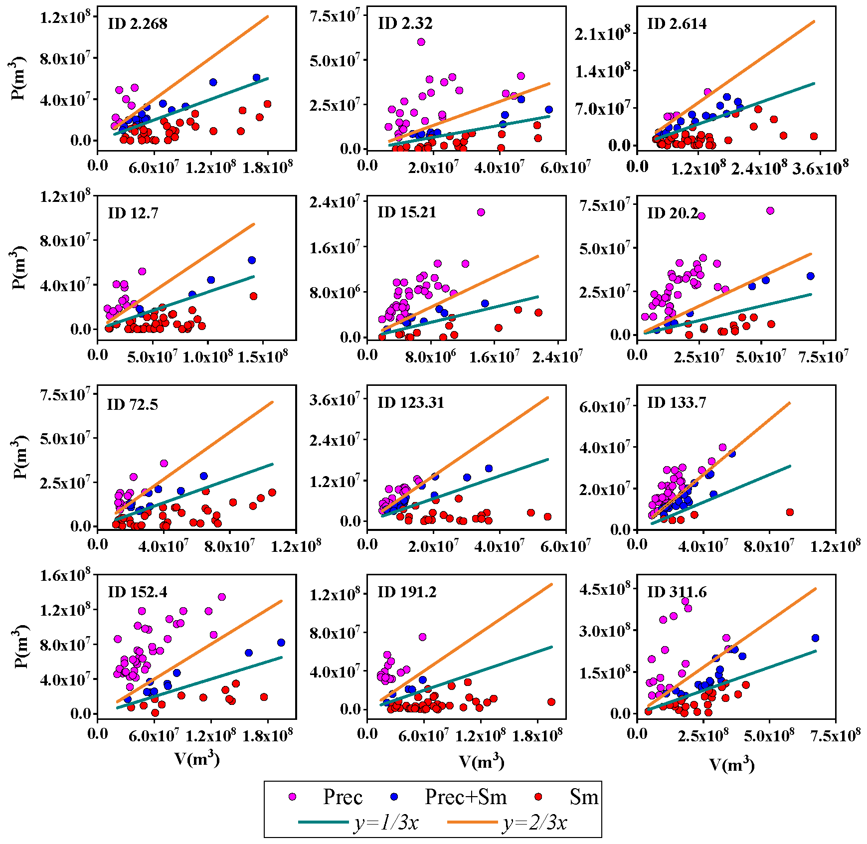
2.2. Two-Component Mixture Distributions Based on Rainfall–Flood Ratio

The mixture distributions were first introduced in flood frequency analysis by Singh and Sinclair [30] and the traditional finite mixture distributions of flood series z t is defined as
f M D z t | θ ,     w = i = 1 u w i f i ( z t | θ t ) i = 1 u w i = 1
where f i z t | θ t is the probability density function of each component; u is the number of considered flood populations; and w i is the weight coefficient of each component, and it indicates the probability that a flood event belongs to each flood population.
The number of component distributions should be determined carefully. If we simply increase the number of component distributions to achieve better fitting qualities, it will reduce the flood samples associated with each component distribution, thus resulting in unreal model and reduce the statistical accuracy of the mixture distributions. Therefore, in practical applications, researchers have assumed that only two FGMs exist and recommended the use of TCMD-T models for flood frequency analysis, which is
f T C M D T z t | θ ,     w = w f 1 z t | θ 1 + 1 w f 2 z t | θ 2
where w and 1 w are the probabilities of flood event z t belonging to flood population 1 and flood population 2, respectively. In this study, we classify the overall flood series in two or three distinct FGMs based on RF indicator in advance; thus, we can construct the TCMD-RF model, probability density function of which is
f T C M D R F z t | θ ,     w = w f R z t | θ 1 + 1 w f S z t | θ 2 w = n R / n R + n S
where f R · and f S · are the probability density functions of rainfall flood and snowmelt flood, respectively. n R and n S are the number of identified rainfall floods and snowmelt floods, respectively. We can see that in TCMD-RF model, the weighting coefficient is determined by its ratio in the whole series before the optimization procedure.

2.2.1. Selection of Component Distributions for Mixture Distributions

In Norway, there typically exist two or three FGMs across the country. Therefore, in this study, we consider three FGMs at most. It should be noted that to guarantee the accuracy of the mixture distributions, for cases where three FGMs are identified but two FGMs are dominant, only two-component mixture distributions will be constructed by discarding the smallest proportion of FGMs. The criterion of rejection is that the number of identified flood events belonging to a certain FGM is less than 20% of the total flood samples. Based on the Norwegian hydrological manual, it is recommended that for hydrological series with a record length of less than 50 years, the mixture of two-parameter probability distributions should be used. Therefore, in this study, the candidate component distributions of the developed mixture distributions are gamma distribution, lognormal distribution and Gumbel distribution. A total of nine different types of TCMD-T models are developed for each station using the three alternative component distributions and considering different FGMs.

2.2.2. Parameters Estimation

For TMCD-T models, in which FGMs are not explicitly classified, the parameters must be jointly estimated, and hydrological researchers have come up with several parameter estimation methods to solve the parameter estimation problem of mixture distributions, such as maximum expectation algorithm (EM), simulated annealing algorithm and meta-heuristic maximum likelihood method (MHML) [3,48]. In this study, the widely used EM method is used for joint parameter estimation of TCMD-T models, while for TCMD-RF, the parameter estimation strategy is different; that is to say, after the explicit classification of FGMs, we only need to estimate the two-parameter distribution for the flood samples associated with each FGM using maximum likelihood method (ML). Then, the constructed component distributions are weighted and summed using the weighting coefficient, which is determined based on the ratio of each FGM to all flood samples, prior to parameter estimation.

2.2.3. Goodness-of-Fitting Test

In this study, a simple AIC criterion is used to test the fitting qualities of mixture models, which is defined as
A I C = 2 l m a x + 2 k
where,   l m a x is the maximum value of log maximum likelihood, and k is the number of parameters to be adjusted, which mainly depends on the number of parameters of the selected component distributions and the model types. The lower of the AIC value, the better the fitting qualities of the model.

2.3. Calculation of Antecedent Precipitation Index

The antecedent precipitation index (API) is the accumulated rainfall volume over a prescribed time period before a given event, and it is typically employed to represent the soil moisture of a basin, which is calculated as follows
A P I t = k P t 1 + k 2 P t 2 + + k T P t T
where, k is the regression coefficient; t is the time when API is estimated. T is the lag time, which can be taken as 1 day, 3 days, 7 days, 15 days and 30 days; P stands for rainfall. In practical applications, researchers often use the combination of k = 0.9 and T = 14 , but it is likely that it is not the most suitable one [49]. Froidevaux et al. [50] proposed the use of regression coefficient k = 0.8 when finding the most suitable delay days of flood trigger in Switzerland. It should be mentioned that longer lag time is suggested for a larger basin and shorter one for a smaller basin. Woldemeskel et al. [51] suggested the use of lag time T ranging from 1 to 7 days and regression coefficient k ranging from 0.4 to 1. Following this suggestion, we adopted 0.8 and 7 days in this study for the regression coefficient and lag time, respectively. The estimation of API is useful for analyzing the relationship between the classified flood types and soil moisture.

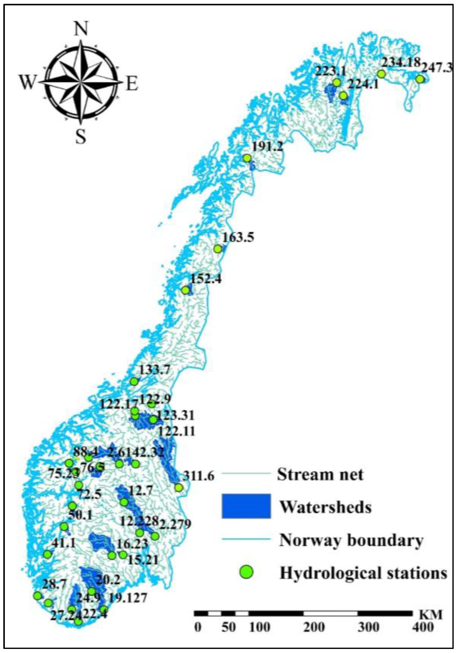
3. Study Area and Data

Norway is located in the northernmost part of northern Europe and the northernmost part of the world, surrounded by sea on three sides. Norway is one of the five Nordic countries, bordering Sweden in the east and Finland and Russia in the northeast. There is great variability in the spatial distribution of climate conditions in Norway, and the annual average temperature ranges from below −3 °C in the northern inland area to above 6 °C in the southern and southwest coastal areas; The average annual precipitation from northeast and central Norway to western Norway generally ranges from about 300 mm to 3500 mm [23,46]. The areas with heavy rainfall are generally in autumn and winter in western Norway and summer in inland areas in eastern Norway. For a long time, the rainfall in Norway falls in the form of snow, which causes a large area of snow to melt when the temperature rises, resulting in a sharp increase in river flow in a short time, resulting in floods. Many studies have shown that in future climate prediction, the total rainfall in the western coastal areas will increase more due to temperature rise than that in the inland areas, especially the rainfall intensity and duration, and the flood frequency caused by rainfall in the western coastal areas will also increase [23,46,52,53].
The temperature, precipitation and runoff data of 34 stations in Norway used in this study are all provided by Norwegian Water Resources and Energy Agency (NVE) (Table 1 and Figure 2), and the river network and watersheds of these 34 hydrological stations are shown in Figure 2. The stations with missing measurements in these three types of observation data were discarded. Finally, 12 stations with different FGMs were selected for further study. From the perspective of geographical location, six stations are located in coastal areas, and the rest are located in internal areas.

4. Results and Discussions

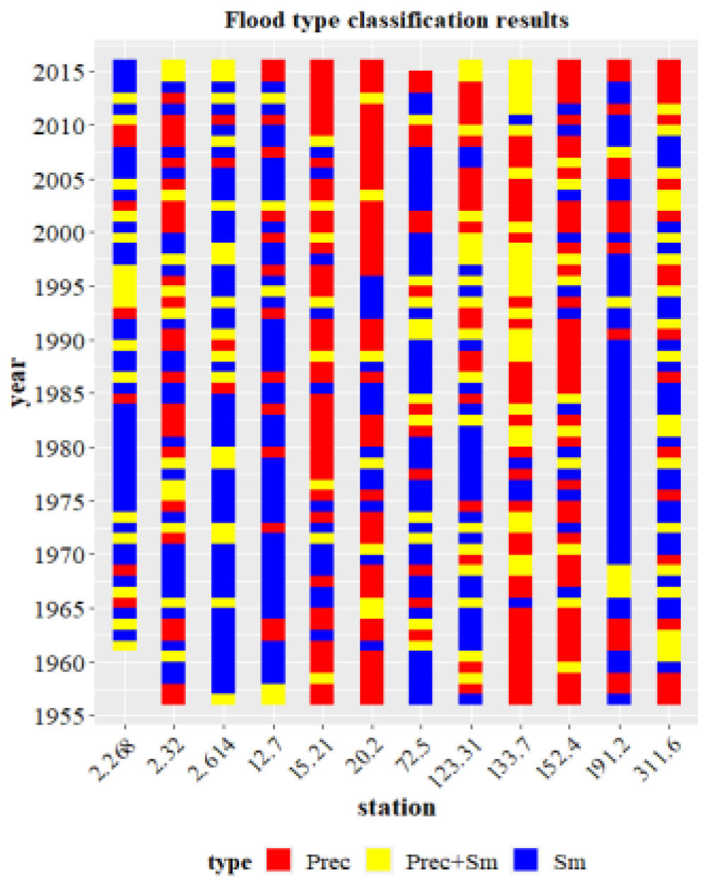
4.1. Classification of Flood Types

As shown in Figure 3, the scatter diagram of rainfall (subtracting evaporation) and flood volume (V) was drawn. Based on the 1/3 V and 2/3 V lines, the 12 selected stations can be clearly divided into three FGMs, namely storm-induced flood, rain-on-snow-induced flood and snowmelt-induced flood, based on the rainfall–flood ratio. Moreover, we can also intuitively see which FGM plays a dominate role in a basin. Among them, floods of seven basins are mainly controlled by storm floods and snowmelt floods, and have less rain-on-snow floods. Interestingly, floods in two basins, Kjeldstad and Nybergsund (ID: 123.31, 311.6), are jointly controlled by all of the three FGMs. The floods of the remaining three basins are dominated by both rain-on-snow floods and one of the other two FGMs. The flood division results show that floods in western coastal areas mainly occur in autumn/winter with heavy rainfall, and a few are caused by snowmelt. In addition, it can be found that most of the selected 12 hydrological stations are dominated by one or two of the three FGMs, which is similar to the previous results of flood classification in Norway [3].
In addition, the identified FGM for each year of the selected 12 stations is shown in Figure 4, which is helpful to see the transition among different FGMs under a changing environment. For example, for station 191.2, there used to be many snowmelt floods before 1990s, but there have been more rainfall-induced floods in recent decades. Additionally, for station 133.7, there are more rain-on-snow flood events in recent decades than previously.

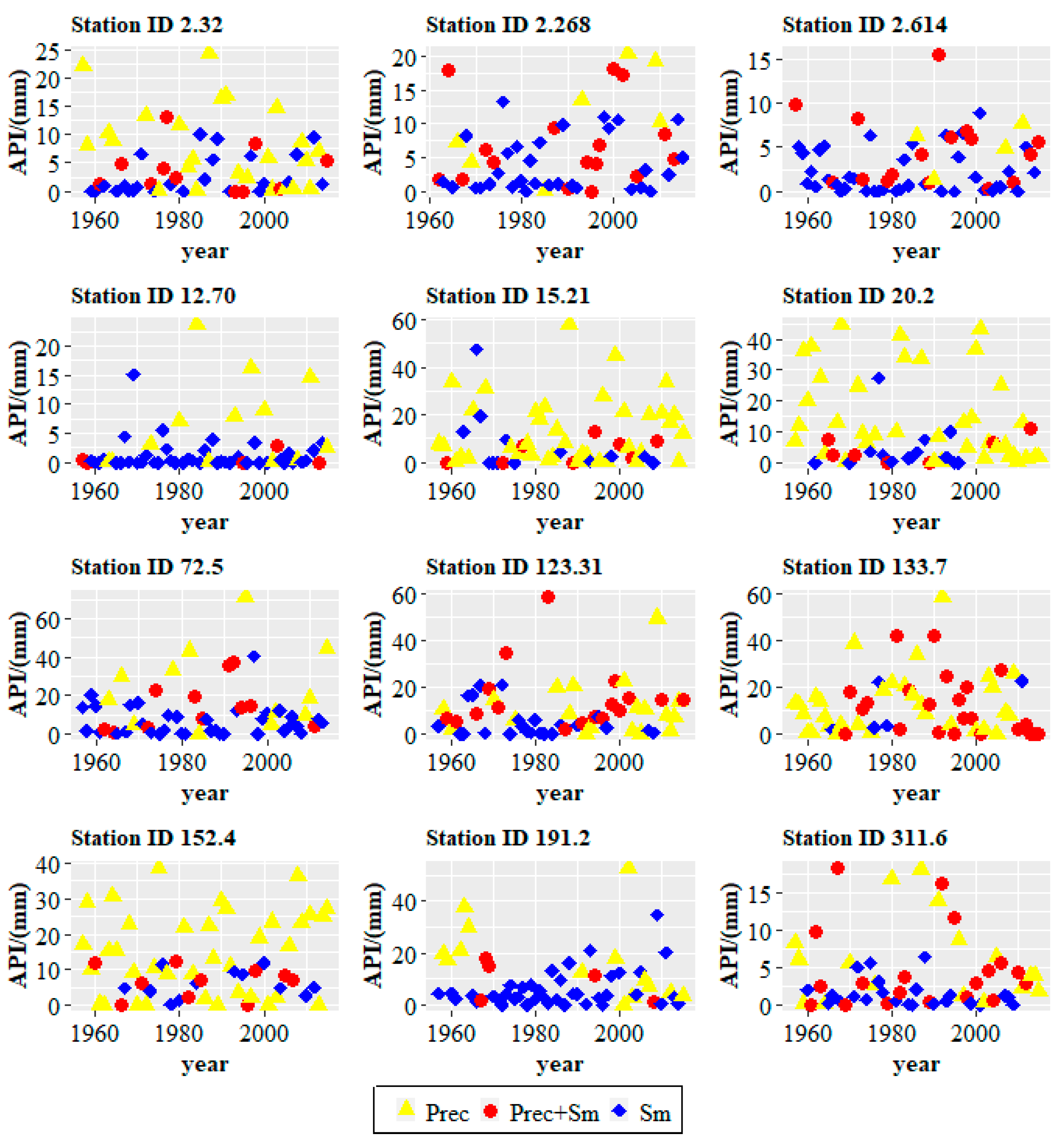
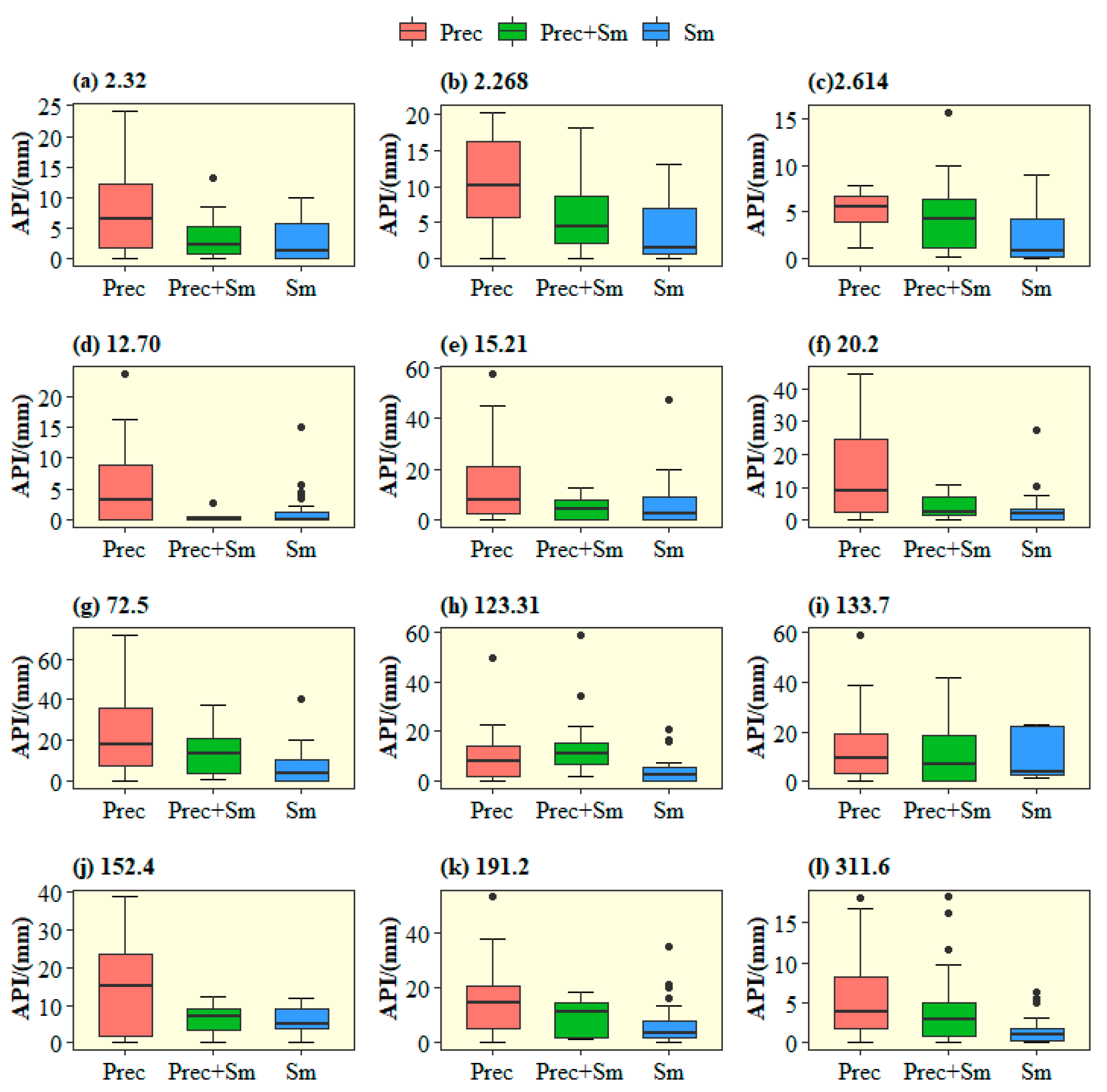
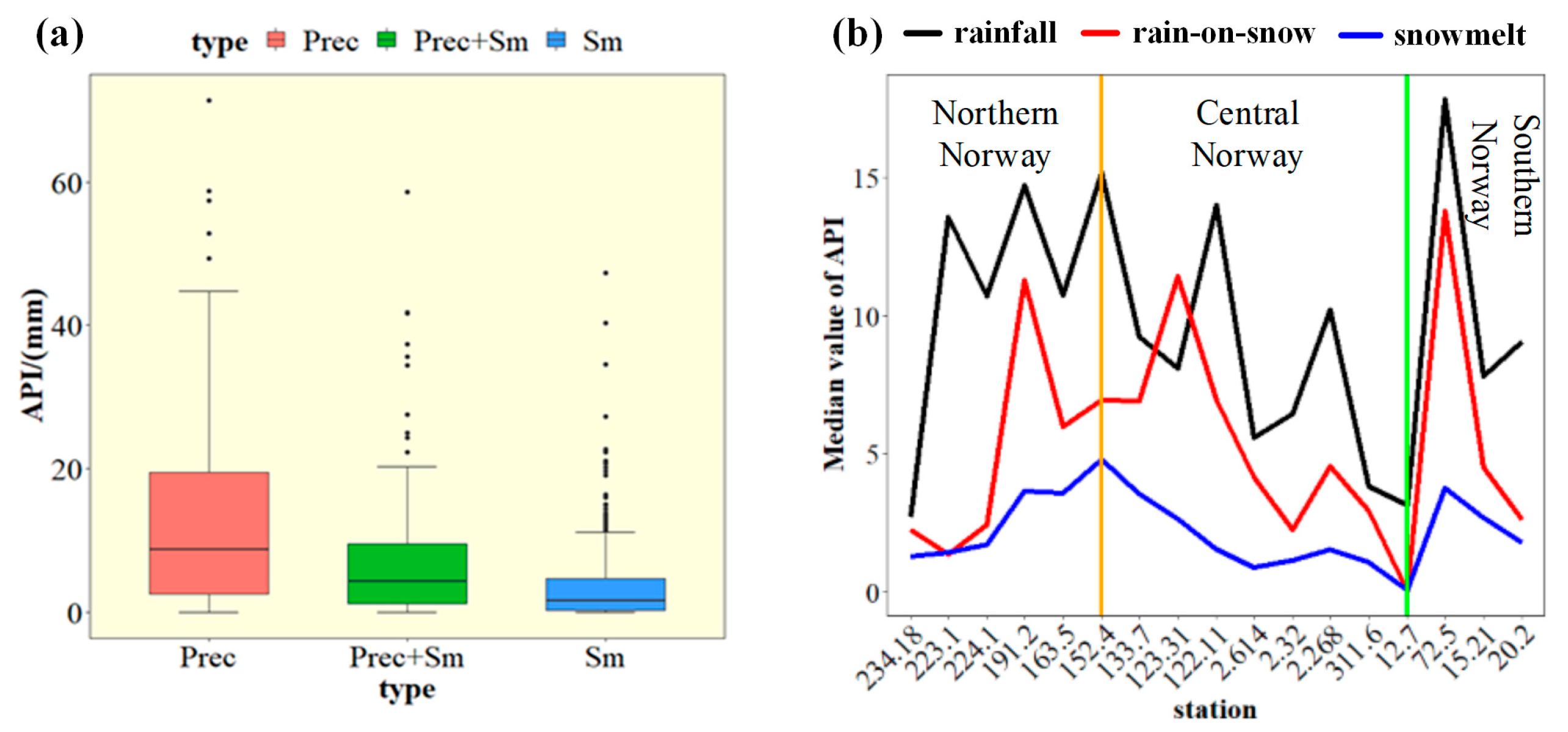
4.2. Relationship between Classified FGMs and API

To bring out the physical meaning of the classified FGMs and check the accuracy of our classification of FGMs, we examined the relationship between each FGM and soil moisture, similar to Hundecha et al. [21]. However, due to the scarcity of soil moisture data, API is used as a proxy of soil moisture in this study. According to the scatter diagram of API values of the three FGMs (Figure 5) and box-plot diagram (Figure 6), it can be seen that the median value of API of rainfall-induced flood is the largest, the median value of API of the identified snowmelt-induced floods is smallest, and the median value of API of rain-on-snow-induced flood lies between them. Moreover, in order to reduce the error caused by short flood series, the average API of each FGM of all 12 selected stations is also analyzed (Figure 7a), and we can obtain the same results. Generally, the above findings are consistent with the formation mechanism of each FGM, and thus further demonstrate the rationality of our classification. In addition, if we arrange the order of all the 34 hydrological stations of Norway according to their geographical spatial location from north to south, we can see that the API median of rain-on-snow floods lies between the rainfall floods and snowmelt floods. Interestingly, we found that the API medians of different FGMs have obvious geographical differences. The API medians are high in northern Norway and decrease in central Norway, and the largest values are typically in Southern Norway (Figure 7b).

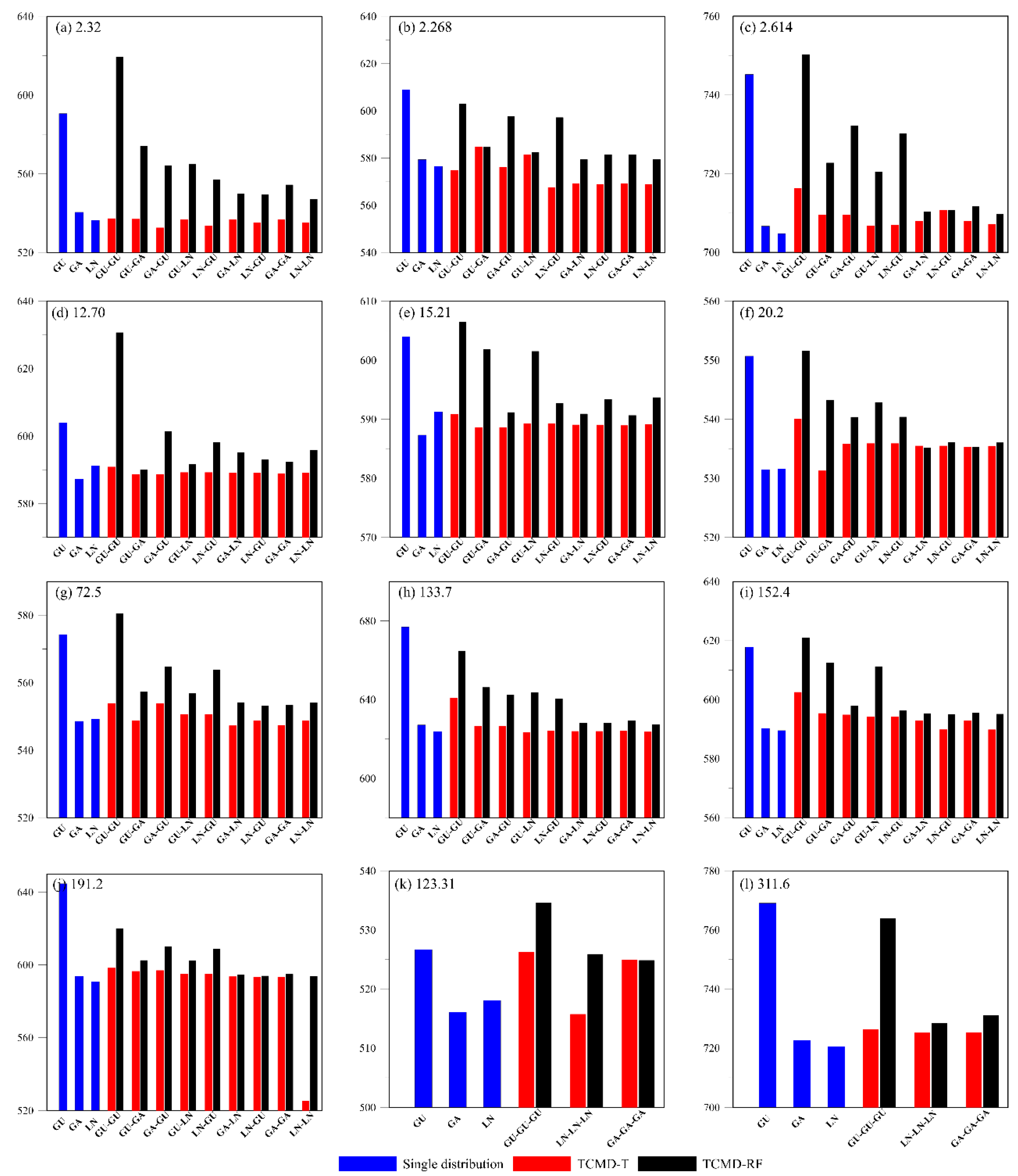
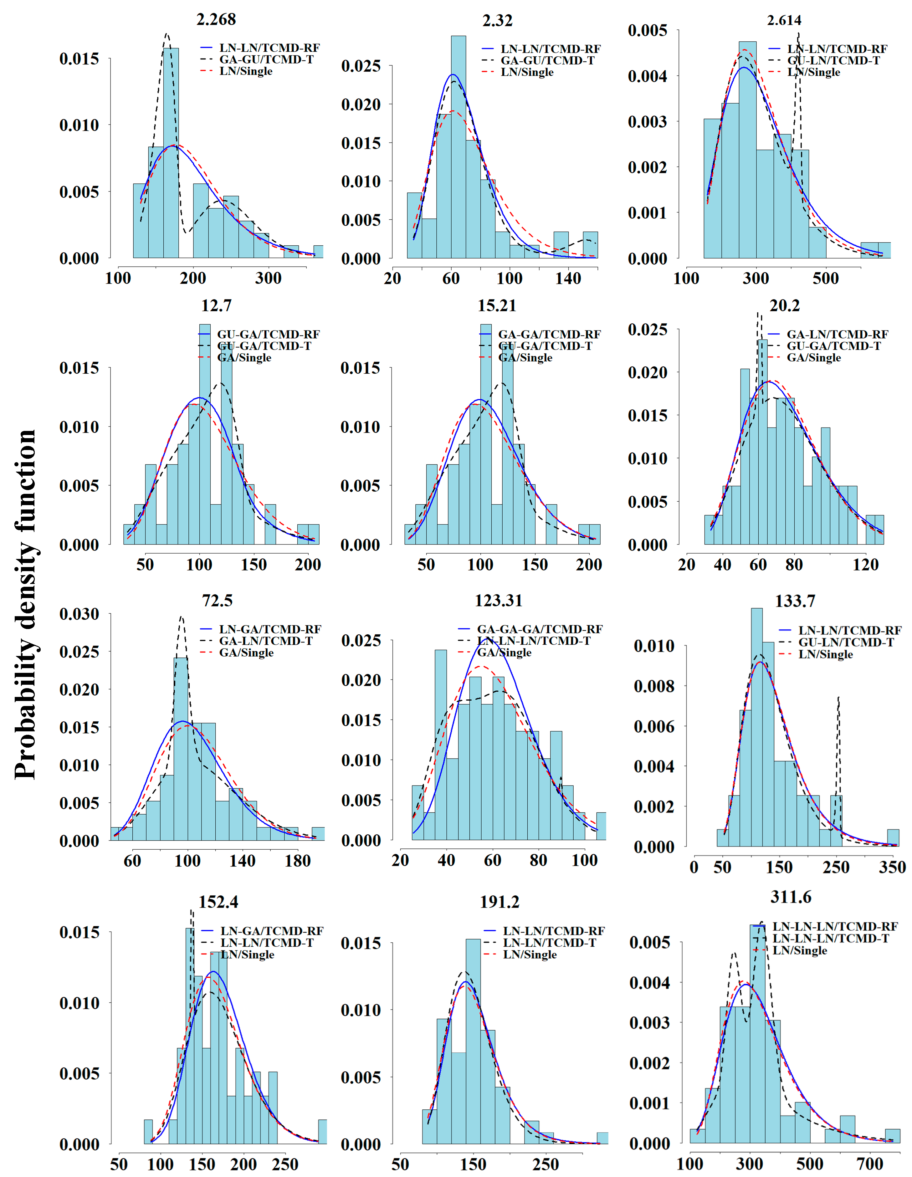
4.3. Mixture Distributions Modeling

Figure 8 summarized the AIC values of the constructed TCMD-T and TCMD-RF models, and also the single distribution model as a baseline. By comparing the performance of the single distribution model and TCMD-T, it can be found that the general performance of the TCMD-T model is better than that of the single distribution model. Among them, the results of Akslen and Øvrevatn stations (ID numbers: 2.268, 191.2) are most convincing. In addition, for cases where single distributions are better, the gap between TCMD-T model and single distribution is very small. However, the performance of TCMD-RF model is not as good as that of TCMD-T model.
In addition to determining the best model by fitting qualities, we also inspected the performance of the mixture models using the probability density functions (Figure 9). The results showed that TCMD-T model is able to better model the probability density of floods, and capture the tail behaviors and multi-modal of flood distribution, and a good example is shown in Akslen station (ID number: 2.268). In this station, it can be seen that the empirical frequency of TCMD-T model is close to the theoretical density curve, and the fitting quality is good. Moreover, the two peaks of the theoretical curve and the empirical frequency are in one-to-one correspondence, and the peak shape of the theoretical density curve is relatively tall and thin (steep). While the other two types of mixture distributions just have a single peak. Through a careful selection of alternative component distributions, TCMD-T is able to better characterize various kinds of skewness and tail behaviors of floods. The immature performance of the TCMD-RF model is thought to be due to the uncertainties associated with flood type classification and arising from the reduced sample size in parameter estimation.

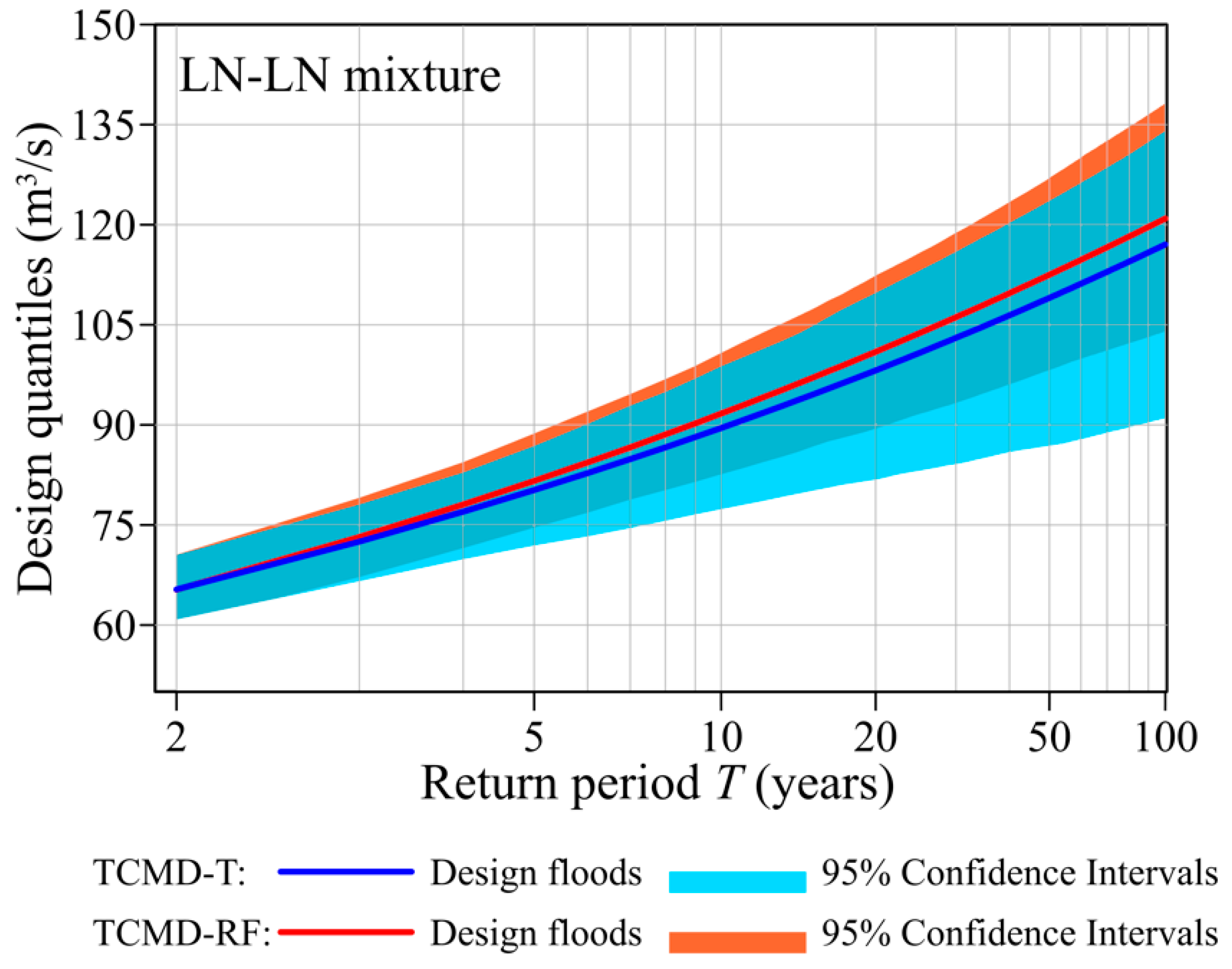
4.4. Estimation of Design Flood Using Mixture Distributions

To compare the difference of TCMD-T and TCMD-RF models in estimating design flood values and associated uncertainties, we take Atnasjø station (ID: 2.32) as an illustration, and estimated the design values for return periods T ∈ [2, 100]. It can be seen that the design flood values that resulted from TCMD-RF are larger than those resulting from TCMD-T when the return period is larger than 5 (Figure 10). To comprehensively compare their difference, we also compute the confidence intervals of design floods using the parametric bootstrap method [54]. A detailed description of this bootstrap method can be found in Yan et al. [3]. As shown in Figure 10, it is found that the CIs of design values yielded by TCMD-RF is always narrower than those of TCMD-T for return period larger than 5, and the largest reduction is about 20%, revealing the advantages of prior classification of FGMs before mixture modeling.

4.5. Discussions

The rainfall–flood ratio method is a simple and feasible method to divide different FGMs in Norway, but it should be noted that there are uncertainties associated with our classification. First, it should be noted that there are different types of FGMs in Norway, and we only consider the two or three main FGMs in a specific basin. However, for cases where there are only two dominant FGMs, we have to abandon some samples, which will reduce the accuracy of any following statistical inference. In addition, restricted by available datasets, we only consider the loss caused by evaporation, but ignore the effects of plant interception and infiltration during rainfall–runoff process. Another level of uncertainty is brought by rainfall-induced floods, mainly occurring in the early summer and autumn, because the previous snowmelt may have saturated the soil moisture when snowmelt-induced floods or rain-on-snow-induced floods occurred, thus promoting surface runoff [21,40]. Moreover, when studying the relationship between flood types and API, we did not consider the influence of frozen soil, and simply used rainfall data to calculate API value following previous studies. This assumption is suitable for rainfall-induced flood, but it should be mentioned that for rain-on-snow-induced floods and snowmelt-induced floods, the infiltration caused by melting snow will also increase soil moisture.
In this study, we tried to improve the physical basis of mixture distributions by classifying different FGMs in advance, and developed the TCMD-RF model. Although the goodness-of-fit of TCMD-RF model is not as good as that of TCMD-T model, which is more flexible in modeling different types of skewness and tail behaviors at the expense of some physical meaning, the uncertainties of the estimated design flood values of TCMD-RF are smaller than those of TCMD-T. The reduction in the estimation uncertainty, larger than 20%, is due to the explicit classification of FGMs of TCMD-RF model. In future, efforts are needed to improve the performance of TCMD-RF model. The flood series for fitting each FGM becomes shorter after the division of FGMs, thus reducing the fitting quality of the model. Therefore, on the one hand, we should collect more flood and hydrometeorological data when developing mixture distributions; on the other hand, we should also try to find more appropriate component distributions.
Finally, another advantage of classification of FGMs is making it possible to analyze the trends of each FGM, and the variation of flood magnitude and frequency for climate change impact studies under a changing environment. Based on this, we can build a more flexible time-varying mixture distribution to characterize the changing properties of each FGM, and attribute the changing of flood characteristics of each FGM to climate factor or human activities, which is expected to enhance both the fitting quality and physical basis of mixture distributions.

5. Conclusions

Classification of flood types and flood frequency analysis using mixture distributions is very important for the flood forecast and control. Using the annual maximum flood series in Norway as illustrations, in this study, we firstly classified distinct FGMs in Norway based on the rainfall–flood ratio, and then constructed the TCMD-RF using the classified flood populations and analyzed whether the performance of the mixture distributions will be improved compared with other TCMD models after the explicit classification of FGMs; finally, we estimated the design flood values and uncertainties associated with TCMD models. The main conclusions of this study are summarized as follows:
(1)
The RF method is a simple and practical method to classify flood types. This method combines both the meteorological information and flood process, and the flood events of the selected 12 stations can be clearly divided into three flood types, namely snowmelt-induced floods, rainfall-induced floods and rain-on-snow floods. Most of the stations are dominated by two of the three flood types.
(2)
Mixture distributions simulation is an effective way to analyze flood frequency. TCMD-T model has the best performance, which can flexibly model various skewness and tail behaviors, and can better capture the double peaks or single peaks of flood probability density, but at the expense of some physical basis of flood generation.
(3)
Although the performance of TCMD-RF model is not as good as TCMD-T model, TCMD-RF can reduce the uncertainties of design flood quantiles by about 20%. The advantage of TCMD-RF model can be attributed to its clear classification of flood types; thus, the weighting coefficients of mixture distributions can be determined before the optimization.

Author Contributions

Conceptualization, L.Y. and L.X.; methodology, L.Z. and C.J.; software, L.Z.; validation, P.Y., W.X. and B.X.; formal analysis, K.Y. and Q.M.; writing—original draft preparation, L.Z. and L.Y.; writing—review and editing, C.-Y.X.; funding acquisition, L.X., C.-Y.X. and L.Y.; All authors have read and agreed to the published version of the manuscript.

Funding

This research was funded by the National Natural Science Foundation of China (No. 51909053, U2240201, 52109002), Visiting Researcher Fund Program of State Key Laboratory of Water Resources and Hydropower Engineering (No. 2019SWG02), and the Research Council of Norway (FRINATEK Project No. 274310 and KLIMAFORSK Project No. 302457), all of which are greatly appreciated.

Data Availability Statement

Data cannot be made publicly available; readers should contact the corresponding author for details.

Acknowledgments

The authors would like to thank the Norwegian Water Resources and Energy Agency (NVE) for providing the runoff, temperature and precipitation data. Great thanks are due to the anonymous reviewers.

Conflicts of Interest

The authors declare no conflict of interest.

References

  1. Tarasova, L.; Merz, R.; Kiss, A.; Basso, S.; Blöschl, G.; Merz, B.; Viglione, A.; Plötner, S.; Guse, B.; Schumann, A. Causative classification of river flood events. Wiley Interdisc. Rev. Water 2019, 6, e1353. [Google Scholar] [CrossRef] [PubMed] [Green Version]
  2. Tarasova, L.; Basso, S.; Wendi, D.; Viglione, A.; Kumar, R.; Merz, R. A process—based framework to characterize and classify runoff events: The event typology of Germany. Water Res. Res. 2020, 56, e2019WR026951. [Google Scholar] [CrossRef]
  3. Yan, L.; Xiong, L.; Ruan, G.; Xu, C.-Y.; Yan, P.; Liu, P. Reducing uncertainty of design floods of two-component mixture distributions by utilizing flood timescale to classify flood types in seasonally snow-covered region. J. Hydrol. 2019, 574, 588–608. [Google Scholar] [CrossRef]
  4. Sultana, T.; Aslam, M.; Raftab, M. Bayesian estimation of 3-component mixture of Gumbel type-Ⅱdistributions under non-informative and informative priors. J. Nat. Sci. Found. Sri Lanka 2017, 45, 287–306. [Google Scholar] [CrossRef]
  5. Rulfová, Z.; Buishand, A.; Roth, M.; Kysely, J. A two-component generalized extreme value distribution for precipitation frequency analysis. J. Hydrol. 2016, 534, 659–668. [Google Scholar] [CrossRef]
  6. Bardsley, W.E. Cautionary note on multicomponent flood distributions for annual maxima. Hydrol. Process. 2016, 30, 3730–3732. [Google Scholar] [CrossRef] [Green Version]
  7. Fischer, S.; Schumann, A.; Schulte, M. Characterisation of seasonal flood types according to timescales in mixture probability distributions. J. Hydrol. 2016, 539, 38–56. [Google Scholar] [CrossRef]
  8. Brunner, M.I.; Viviroli, D.; Sikorska, A.E.; Vannier, O.; Favre, A.C.; Seibert, J. Flood type specific construction of synthetic design hydrographs. Water Resour. Res. 2017, 53, 1390–1406. [Google Scholar] [CrossRef] [Green Version]
  9. Alila, Y.; Mtiraoui, A. Implications of heterogeneous flood-frequency distributions on traditional stream-discharge prediction techniques. Hydrol. Process. 2002, 16, 1065–1084. [Google Scholar] [CrossRef]
  10. Qu, C.; Li, J.; Yan, L.; Yan, P.; Cheng, F.; Lu, D. Non-stationary flood frequency analysis using cubic B-spline-based GAMLSS model. Water 2020, 12, 1867. [Google Scholar] [CrossRef]
  11. Jiang, C.; Xiong, L.; Yan, L.; Dong, J.; Xu, C.-Y. Multivariate hydrologic design methods under nonstationary conditions and application to engineering practice. Hydrol. Earth Syst. Sci. 2019, 23, 1683–1704. [Google Scholar] [CrossRef] [Green Version]
  12. Xiong, L.; Yan, L.; Du, T.; Yan, P.; Li, L.; Xu, W. Impacts of climate change on urban extreme rainfall and drainage infrastructure performance: A case study in Wuhan City, China. Irrig. Drain. 2019, 68, 152–164. [Google Scholar] [CrossRef]
  13. Milly, P.C.D.; Betancourt, J.; Falkenmark, M.; Hirsch, R.M.; Kundzewicz, Z.W.; Lettenmaier, D.P.; Stouffer, R.J.; Dettinger, M.D.; Krysanova, V. On critiques of “Stationarity is Dead: Whither Water Management?”. Water Resour. Res. 2015, 51, 7785–7789. [Google Scholar] [CrossRef] [Green Version]
  14. Xu, W.; Jiang, C.; Yan, L.; Li, L.; Liu, S. An adaptive Metropolis-Hastings optimization algorithm of Bayesian estimation in non-stationary flood frequency analysis. Water Resour. Manag. 2018, 32, 1343–1366. [Google Scholar] [CrossRef]
  15. Yan, L.; Xiong, L.; Liu, D.; Hu, T.; Xu, C.-Y. Frequency analysis of nonstationary annual maximum flood series using the time-varying two-component mixture distributions. Hydrol. Process. 2017, 31, 69–89. [Google Scholar] [CrossRef]
  16. Yan, L.; Li, L.; Yan, P.; He, H.; Li, J.; Lu, D. Nonstationary flood hazard analysis in response to climate change and population growth. Water. 2019, 11, 1811. [Google Scholar] [CrossRef] [Green Version]
  17. Vogel, R.M.; Yaindl, C.; Walter, M. Nonstationarity: Flood magnification and recurrence reduction factors in the United States 1. J. Amer.Water Res. Assoc. 2011, 47, 464–474. [Google Scholar] [CrossRef]
  18. Yang, L.; Wang, L.; Li, X.; Gao, J. On the flood peak distributions over China. Hydrol. Earth Syst. Sci. 2019, 23, 5133–5149. [Google Scholar] [CrossRef] [Green Version]
  19. Barth, N.A.; Villarini, G.; Nayak, M.A.; White, K. Mixed populations and annual flood frequency estimates in the western United States: The role of atmospheric rivers. Water Resour. Res. 2017, 53, 257–269. [Google Scholar] [CrossRef]
  20. Barth, N.A.; Villarini, G.; White, K. Accounting for mixed populations in flood frequency analysis: Bulletin 17C perspective. J. Hydrol. Eng. 2019, 24, 04019002. [Google Scholar] [CrossRef]
  21. Hundecha, Y.; Parajka, J.; Viglione, A. Flood type classification and assessment of their past changes across Europe. Hydrol. Earth Syst. Sci. Discuss. 2017. [Google Scholar] [CrossRef] [Green Version]
  22. Vormoor, K.; Lawrence, D.; Heistermann, M.; Bronstert, A. Climate change impacts on the seasonality and generation processes of floods–projections and uncertainties for catchments with mixture snowmelt/rainfall regimes. Hydrol. Earth Syst. Sci. 2015, 19, 913–931. [Google Scholar] [CrossRef] [Green Version]
  23. Vormoor, K.; Lawrence, D.; Schlichting, L.; Wilson, D.; Wong, W.K. Evidence for changes in the magnitude and frequency of observed rainfall vs. snowmelt driven floods in Norway. J. Hydrol. 2016, 538, 33–48. [Google Scholar] [CrossRef]
  24. Wyżga, B.; Kundzewicz, Z.W.; Zawiejska, V.R.V.J. Flood generation mechanisms and changes in principal drivers. In Flood Risk in the Upper Vistula Basin; Springer Cham: New York, NY, USA, 2016; pp. 55–75. [Google Scholar]
  25. Smith, J.A.; Villarini, G.; Baeck, M.L. Mixture distributions and the hydroclimatology of extreme rainfall and flooding in the eastern United States. J. Hydrometeorol. 2011, 12, 294–309. [Google Scholar] [CrossRef]
  26. Jiang, C.; Xiong, L.; Xu, C.-Y.; Yan, L. A river network—based hierarchical model for deriving flood frequency distributions and its application to the Upper Yangtze Basin. Water Resour. Res. 2021, 57, e2020WR029374. [Google Scholar] [CrossRef]
  27. Li, J.; Zheng, Y.; Wang, Y.; Zhang, T. Improved mixture distribution model considering historical extraordinary floods under changing environment. Water 2018, 10, 1016. [Google Scholar] [CrossRef] [Green Version]
  28. Zeng, H.; Feng, P.; Li, X. Reservoir flood routing considering the non-stationarity of flood series in north China. Water Resour. Manag. 2014, 28, 4273–4287. [Google Scholar] [CrossRef]
  29. McLachlan, G.J.; Lee, S.X.; Rathnayake, S.I. Finite mixture models. Annu. Rev. Stat. Appl. 2019, 6, 355–378. [Google Scholar] [CrossRef]
  30. Singh, K.P.; Sinclair, R.A. Two-distribution method for flood frequency analysis. J. Hydraul. Division 1972, 98, 28–44. [Google Scholar] [CrossRef]
  31. Grego, J.M.; Yates, P.A. Point and standard error estimation for quantiles of mixed flood distributions. J. Hydrol. 2010, 391, 289–301. [Google Scholar] [CrossRef]
  32. Kuang, Y.; Xiong, L.; Yu, K.X.; Liu, P.; Xu, C.-Y.; Yan, L. Comparison of first-order and second-order derived moment approaches in estimating annual runoff distribution. J. Hydrol. Eng. 2018, 23, 04018034. [Google Scholar] [CrossRef]
  33. Yan, L.; Xiong, L.; Luan, Q.; Jiang, C.; Yu, K.; Xu, C.-Y. On the applicability of the expected waiting time method in nonstationary flood design. Water Resour. Manag. 2020, 34, 2585–2601. [Google Scholar] [CrossRef]
  34. Turkington, T.; Breinl, K.; Ettema, J.; Alkema, D.; Jetten, V. A new flood type classification method for use in climate change impact studies. Weather. Clim. Extrem. 2016, 14, 1–16. [Google Scholar] [CrossRef] [Green Version]
  35. Gain, A.K.; Apel, H.; Renaud, F.G.; Giupponi, C. Thresholds of hydrologic flow regime of a river and investigation of climate change impact—The case of the Lower Brahmaputra River Basin. Clim. Chang. 2013, 120, 463–475. [Google Scholar] [CrossRef] [Green Version]
  36. Garner, G.; Van Loon, A.F.; Prudhomme, C.; Hannah, D.M. Hydroclimatology of extreme river flows. Freshw. Biol. 2015, 60, 2461–2476. [Google Scholar] [CrossRef]
  37. Sikorska, A.E.; Viviroli, D.; Seibert, J. Flood-type classification in mountainous catchments using crisp and fuzzy decision trees. Water Resources. Res. 2015, 51, 7959–7976. [Google Scholar] [CrossRef]
  38. Yan, L.; Xiong, L.; Wang, J. Analysis of storm runoff simulation in typical urban region of Wuhan based on SWMM. J. Water Resour. Res 2014, 3, 216–228. [Google Scholar] [CrossRef]
  39. Prudhomme, C.; Genevier, M. Can atmospheric circulation be linked to flooding in Europe. Hydrol. Process. 2011, 25, 1180–1990. [Google Scholar] [CrossRef] [Green Version]
  40. Merz, R.; Blöschl, G. A process typology of regional floods. Water Resour. Res. 2003, 39, 1340. [Google Scholar] [CrossRef]
  41. Duckstein, L.; Bárdossy, A.; Bogárdi, I. Linkage between the occurrence of daily atmospheric circulation patterns and floods: An Arizona case study. J. Hydrol. 1993, 143, 413–428. [Google Scholar] [CrossRef]
  42. Hirschboeck, K.K. Hydroclimatically-defined mixture distributions in partial duration flood series. In Proceedings of the International Symposium on Flood Frequency and Risk Analyses, Louisiana State University, Baton Rouge, LA, USA, 14–17 May 1986. [Google Scholar]
  43. Zhai, X.; Guo, L.; Zhang, Y. Flash flood type identification and simulation based on flash flood behavior indices in China. Sci. China Earth Sci. 2021, 64, 1140–1154. [Google Scholar] [CrossRef]
  44. Gaál, L.; Szolgay, J.; Kohnová, S.; Parajka, J.; Merz, R.; Viglione, A.; Blöschl, G. Flood timescales: Understanding the interplay of climate and catchment processes through comparative hydrology. Water Resour. Res. 2012, 48, W04511. [Google Scholar] [CrossRef]
  45. Lu, W.; Lei, H.; Yang, W.; Yang, J.; Yang, D. Comparison of floods driven by tropical cyclones and monsoons in the southeastern coastal region of China. J. Hydrometeorol. 2020, 21, 1589–1603. [Google Scholar] [CrossRef]
  46. Hanssen-Bauer, I.; Førland, E.J.; Haddeland, I.; Hisdal, H.; Mayer, S.; Nesje, A.; Nilsen, J.E.Ø.; Sandven, S.; Sandø, A.B.; Sorteberg, A.; et al. Climate in Norway 2100—A knowledge base for climate adaption. Nor. Cent. Clim. Serv. 2017, 48. [Google Scholar]
  47. Sikorska-Senoner, A.E.; Seibert, J. Flood-type trend analysis for alpine catchments. Hydrol. Sci. J. 2020, 65, 1281–1299. [Google Scholar] [CrossRef]
  48. Yan, L.; Xiong, L.; Guo, S.; Xu, C.-Y.; Xia, J.; Du, T. Comparison of four nonstationary hydrologic design methods for changing environment. J. Hydrol. 2017, 551, 132–150. [Google Scholar] [CrossRef]
  49. Heggen, J.R. Normalized antecedent precipitation index. J. Hydrol. Eng. 2001, 6, 377–381. [Google Scholar] [CrossRef]
  50. Froidevaux, P.; Schwanbeck, J.; Weingartner, R.; Chevalier, C.; Martius, O. Flood triggering in Switzerland: The role of daily to monthly preceding precipitation. Hydrol Earth Syst. Sci. 2015, 19, 3903–3924. [Google Scholar] [CrossRef] [Green Version]
  51. Woldemeskel, F.; Sharma, A. Should flood regimes change in a warming climate? The role of antecedent moisture conditions. Geophys. Res. Lett. 2016, 43, 7556–7563. [Google Scholar] [CrossRef]
  52. Hegdahl, T.J.; Engeland, K.; Müller, M.; Sillmann, J. An Event-Based Approach to Explore Selected Present and Future Atmospheric River–Induced Floods in Western Norway. J. Hydrol. 2020, 21, 2003–2021. [Google Scholar] [CrossRef]
  53. Sorteberg, A.; Lawrence, D.; Dyrrdal, A.V.; Mayer, S.; Engeland, K. Climate changes in short duration extreme precipitation and rapid onset flooding—Implications for design values. Nor. Cent. Clim. Serv. 2018, 143. [Google Scholar]
  54. Efron, B. Bootstrap methods: Another Look at the Jackknife. Ann. Stat. 1979, 7, 1–26. [Google Scholar] [CrossRef]
Figure 1. Schematic diagram of the rainfall–runoff process. V r and V q are the rainfall volume and runoff volume for the period before flood peak, respectively.
Remotesensing 15 00401 g001
Figure 2. The location map of the 34 basins throughout Norway.
Remotesensing 15 00401 g002
Figure 3. Classification results of FGMs using the rainfall–flood ratio indicators. The flood events are classified by rainfall–flood ratio, indicated by 1/3 and 2/3 lines. Pink dots represent floods caused by rainfall, blue dots represent the interaction of rainfall and snowmelt, and red dots represent floods induced by snowmelt.
Remotesensing 15 00401 g003
Figure 4. Results of classification of flood types. The yellow rectangle represents the rainfall floods (Prec), the green rectangle is rain-on-snow induced floods (Prec+Sm), and the blue rectangle is the snowmelt flood (Sm).
Remotesensing 15 00401 g004
Figure 5. The API values associated with each flood event and flood types. The yellow triangle represents API value of rainfall floods (Prec), red dot represents API value of rain-on-snow floods (Prec + Sm), and diamond represents snowmelt flood (Sm).
Remotesensing 15 00401 g005
Figure 6. Box-plot of the API for different FGMs. The thick black line in the middle of the box is the API median of a certain flood type. The black dots are outliers.
Remotesensing 15 00401 g006
Figure 7. Relationship between API median and identified flood types. (a) box-plot of the API for different FGMs averaged by all stations; (b) relationship between API median and its geographical location for each FGM.
Remotesensing 15 00401 g007
Figure 8. The AIC values of the single distribution model and mixture distributions, namely TCMD-T and TCMD-RF, with various component distributions.
Remotesensing 15 00401 g008
Figure 9. Histogram of floods and probability density function of TCMD-T, TCMD-RF and single distribution.
Remotesensing 15 00401 g009
Figure 10. Design values and associated uncertainties using TCMD-T (blue line) and TCMD-RF (red line) with LN-LN mixture type.
Remotesensing 15 00401 g010
Table 1. The information of 34 hydrological stations in Norway. The stations with bold fonts were selected for further study.
Station IDNameArea (km2)Data Period Q ¯ m m / y r P ¯ r e c ( mm / yr ) t ¯ e m p ° C
2.268Akslen789.31934–2015992.71195.6−3.18
2.279Kråkfoss435.21966–2015613.01030.72.69
2.291Tora262.11967–20151511.11542.5−2.30
2.32Atnasjø463.31917–2015705.4859.0−2.10
2.614Rosten18331917–2015558.6884.3−1.31
12.228Kistefoss37031917–2015502.31035.51.11
12.7Etna570.31920–2015541.61177.0−0.58
15.21Jondalselv1261920–2015750.51212.82.26
16.23Kirkevollbru3845.41906–2015755.21475.4−0.66
19.127Rygenetotal3946.41900–2015930.81512.73.43
20.2Austenå276.41925–20151224.81872.12.42
22.4Kjæøemo1757.71897–20151490.22266.33.62
24.9Tingvatn272.21923–20151755.22628.53.56
27.24Helleland184.71897–20152338.03430.24.69
28.7Haugland139.41919–20151520.72082.96.31
41.1Stordalsvatn130.71913–20153093.84029.73.93
50.1Hølen232.71923–20151596.82671.50.33
72.5Brekkebru268.21944–20141940.42383.8−0.36
75.23Krokenelv45.91965–20151537.71976.30.70
76.5Nigardsbrevatn65.31963–20153082.03221.6−1.34
88.4Lovatn234.91900–20152148.72872.30.36
122.11Eggafoss655.21941–2015833.51160.1−0.03
122.17Hugdalbru545.91973–2015750.21136.61.45
122.9Gaulfoss3085.91958–2015849.01182.30.78
123.31Kjeldstad1431930–20151608.01441.72.21
133.7Krinsvatn206.61916–20151903.32337.03.80
152.4Fustvatn525.71909–20151933.02365.01.60
163.5Junkerdalselv4221938–20151079.61294.2−1.44
191.2Øvrevatn5261914–20151294.41642.6−0.70
223.1Stabburselv1067.31924–2015641.1697.7−1.82
224.1Skoganvarre940.71922–2014504.0598.2−2.33
234.18Polmak14161.41912–2015379.1527.9−3.01
247.3Karpelva128.91928–2015556.9668.5−0.76
311.6Nybergsund4424.91909–2015493.2894.3−0.90
Disclaimer/Publisher’s Note: The statements, opinions and data contained in all publications are solely those of the individual author(s) and contributor(s) and not of MDPI and/or the editor(s). MDPI and/or the editor(s) disclaim responsibility for any injury to people or property resulting from any ideas, methods, instructions or products referred to in the content.

