Thermal Mapping from Point Clouds to 3D Building Model Facades

Abstract

Thermal inspection of buildings regarding efficient energy use is an increasing need in today’s energy-demanding world. This paper proposes a framework for mapping temperature attributes from thermal point clouds onto building facades. The goal is to generate thermal textures for three-dimensional (3D) analysis. Classical texture generation methods project facade images directly onto a 3D building model. Due to the limited level of detail of these models, projection errors occur. Therefore, we use point clouds from mobile laser scanning extended by intensities extracted from thermal infrared (TIR) image sequences. We are not using 3D reconstructed point clouds because of the limited geometric density and accuracy of TIR images, which can lead to poor 3D reconstruction. We project these thermal point clouds onto facades using a mapping algorithm. The algorithm uses a nearest neighbor search to find an optimal nearest point with three different approaches: “Minimize angle to normal”, “Minimize perpendicular distance to normal”, and “Minimize only distance”. Instead of interpolation, nearest neighbor is used because it retains the original temperature values. The thermal intensities of the optimal nearest points are weighted by resolution layers and mapped to the facade. The approach “Minimize perpendicular distance to normal” yields the finest texture resolution at a reasonable processing time. The accuracy of the generated texture is evaluated based on estimating the shift of the window corner points from a ground truth texture. A performance metric root-mean-square deviation (RMSD) value that measures this shift is calculated. In terms of accuracy, the nearest neighbor method outperformed bilinear interpolation and an existing TIR image-based texturing method.

1. Introduction

Over the last few years, thermography has gained numerous applications in terms of studying the energy situation in the world. Since the industrial revolution, a large part of the world’s population has shifted to urban locations. As a result, the built environment expanded quickly, producing significant carbon dioxide emissions from the energy used in buildings. Therefore, energy consumption by buildings has become a widely spoken topic. The scientific community has grown interested in infrared radiation (IR) thermography [1], especially because it is cost-effective and can provide images of different building elements representing the surface temperature. Buildings’ thermal radiance is recorded using thermal infrared (TIR) cameras, a time-efficient and economical tool for monitoring leakage and energy usage. It is also a non-contact and non-destructive method for thermal analysis. Thermal analysis [2] is necessary for detecting patterns such as the inhomogeneous distribution of wall materials, anomalies, heating system pipes, internal cracks, structural damages [3], leakages, moisture [4], failure of electrical circuits, air conditioning, ventilation, etc., which are typically hidden from the building’s surface. Traditional methods of monitoring the thermal signature are manually looking at a series of TIR images captured from different viewing positions. Some drawbacks of directly using the images are that they include occluded objects and also require a significant overlap between multi-view images. Also, there can be temporal and illumination changes in transition areas between image acquisitions. Therefore, including a three-dimensional (3D) spatial reference containing thermal information in the building model can increase the scope of thermal building inspection [5]. For complex buildings, instead of looking at isolated facades, the whole structure can be observed as a single unit. We can locate the anomalies with a 3D reference to the building and perform change detection and observation of dynamic processes more efficiently. Information from the inside of walls can be connected to the outside to identify energy loss.

Now, there can be different ways to represent 3D information, such as adding thermal textures to 3D geometric building models [6,7] or representing the thermal information in the form of voxels or meshes [8] or thermal point clouds [9,10]. Some researchers in the past have devoted themselves to generating some of these kinds of representations. One thing to remember while using archived building models is that we can update the models from time to time, and acquiring the latest representation of buildings can be labor-intensive and time-consuming. Moreover, the levels of detail (LoDs) imply the precise geometric depiction of the building model. Also, the bigger vision should be to scale-up thermal models to vast areas like cities, states, or even countries.

The goal of our project is to enrich building models with thermal information. Hence, we have worked on generating textures by projecting point clouds to facades. Otherwise, we could have directly used 3D thermal point clouds. Also, later, for thermal analysis, we will use Neural Networks for image interpretation in the thermal textures. The interpretation of images is also more convenient than point clouds. Additionally, point clouds also contain occlusions, outliers, noise, and unwanted data. Some of this information is irrelevant and we do not want to process these extra information. Textures do not include this unwanted information, but only contain the information relevant to a particular facade structure.

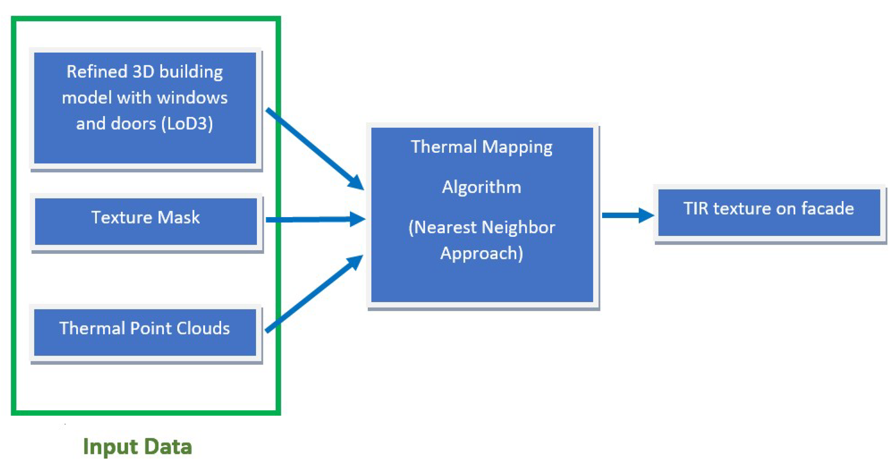
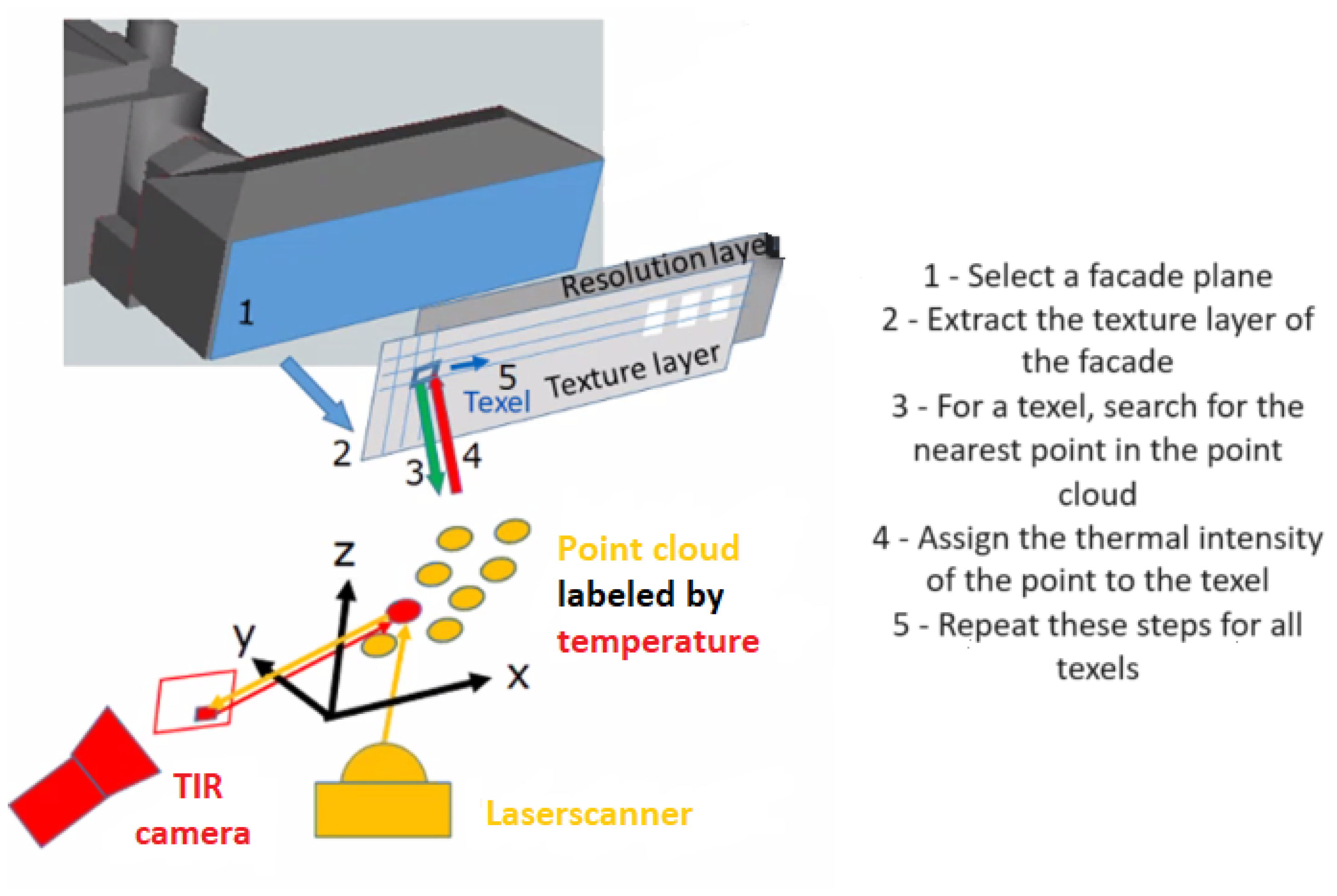
This paper contributes a novel technique to texture facades of 3D building models using thermal point clouds. We assume that Mobile Laser Scanning (MLS) point clouds and thermal images were recorded in one measurement campaign and are fused to a thermally enriched 3D point cloud. We further assume that the point cloud was already used to refine the original building model by adding elements like windows and doors. A mapping algorithm takes the texture layer of the facade. For each texture pixel (texel), the algorithm finds the nearest optimal point closest to the vertical of the facade and which has a temperature value. A resolution layer weights the thermal intensities of all optimal points before assigning them to the texture layer. The generated TIR texture is enhanced and finally applied to the facade. This paper is structured into different parts. Section 1 introduces the overall problem statement, Section 2 discusses the related research conducted previously, Section 3 describes in detail the methodology workflow, Section 4 describes the test datasets and input data preparation, Section 5 presents the implementation results and analysis, and Section 6 finally draws conclusions and introduces future work.

In our mapping algorithm, we can compute the texel intensity using different methods such as nearest neighbor point, bilinear interpolation, cubic spline interpolation, etc. The primary reason that we have selected the nearest neighbor point is to keep the original temperature values. Nearest neighbor ensures the original temperature but at a slightly shifted position (lower geometric accuracy). On the other hand, interpolation has an estimated (weighted mean) temperature, but higher geometric accuracy (no geometric shift). An interpolation would have generated intermediate average values via some weighting criteria, which would have changed the original values. Another advantage of using the nearest neighbor is its simplicity, as we take the nearest point based on a distance metric without further calculating average values based on some complicated rules. But the downside of using the nearest neighbor approach is that some texels with no corresponding vertical neighbor points are left empty, so the generated texture image has some blank texels. Interpolation would have filled up all those empty texels. Also, with interpolation, we can further increase the resolution to obtain finer texels, but with the nearest neighbor, this will result in more blank texels. Hence, there is a trade-off between selecting the method that provides the real temperature at a slightly shifted position versus the method that provides an estimated/interpolated temperature with no shift.

The main innovation in this paper is the usage of thermal point clouds to generate thermal textures. Previously, researchers worked on generating thermal textures directly from TIR images or point clouds reconstructed from TIR images. Some classical texture generation methods project facade images directly onto the 3D building models. Due to the limited level of detail of these simplified building models, projection errors occur. Some other drawbacks, such as limited geometric density and lower resolution/accuracy of TIR images, lead to poor 3D reconstruction or blurry textures. Also, TIR images include reflections from window glasses and occlusions. Objects in the TIR domain show radiometric behavior, which causes blurred edges in the generated textures. In Section 2, we discussed the drawbacks of facade texture generation from TIR images. Therefore, to overcome the limitations of these methods, we are using thermal point clouds prepared by extending laser scanner point clouds with intensities from TIR images. The reason why we used point clouds instead of images for texture generation is because of TIR image interpretation challenges, discussed in detail in Section 2. We projected the thermal point clouds to building facades by using a mapping algorithm. The mapping algorithm uses a nearest neighbor approach. Later, we also implemented bilinear interpolation and compared that with the nearest neighbor. We also investigated different approaches for the nearest neighbor search to calculate the intensities, compared and analyzed them, deduced the best-suited approach, and finally presented a performance metric of the results.

2. Related Work

Some research has been conducted on preparing 3D thermal point clouds from different sources. Ref. [11] reconstructed 3D point clouds containing TIR attributes using Structure from Motion (SfM) techniques with multi-view stereo-principle. The images were taken from Unmanned Aerial Vehicles (UAVs). Low-quality thermal images are challenging for this method since there must be enough detected features, especially when an uncooled camera captures the image. Ref. [12] proposes an automated approach to register thermal with red, green, and blue (RGB) point clouds reconstructed independently via SfM. Normalizing the point cloud scale is the first step in the registration procedure. Global registration using calibration data and SfM output is followed by fine registration using an iterative closest point (ICP) optimization variant. Ref. [13] generated dense point clouds directly from TIR images by automatically orienting sequences of images taken from UAVs. However, if RGB images are additionally available, dense point clouds are generated from RGB data. Then, the ICP algorithm is used to align the point clouds, a mesh is generated from the RGB point cloud, and, finally, a 3D model is created by mapping the texture from TIR images. Ref. [14] superimposes thermal information onto each point on 3D structures reconstructed with Direct Sparse Odometry (DSO) using RGB images to create a 3D thermal map. The RGB and TIR cameras are mounted on a stereo rig and their relative pose is estimated. Depth images from RGB and TIR cameras are matched based on mutual information. Then, the point cloud’s scale is estimated corresponding to extrinsic parameters between both cameras to perform the superimposition. Ref. [15] generated point clouds using SfM using cell phone images. Then, the temperature information was projected to the generated point clouds by utilizing a thermal camera’s relative position data. Ref. [16] used a “bi-camera” system to integrate RGB and IR cameras and then performed thermal 3D mapping by registering the images into a terrestrial laser scanner (TLS) reference system.

Texturing building facades with thermal images was attempted by [17]. Here, 3D models generated from terrestrial laser scanners are taken, and then RGB and TIR image blocks are mapped to the model. It uses accurate photogrammetric orientation via bundle adjustment that integrates TIR and RGB data. Ref. [18] creates a 3D thermal map of a building using three sensors: a color camera, a 3D laser scanner, and a thermal camera setup in a robot. The sensors are automatically co-calibrated, and one highly accurate 3D model incorporating data from all the sensors is created to depict the heat distribution. Ref. [19] maps roofs by fusing thermal and visible point clouds. The point clouds are generated from their respective thermal and visible UAV images. The point clouds are then geo-referenced using control points and are co-registered. Building roofs are extracted from visible point clouds and thermal point clouds, which are combined to create a fused dense point cloud. Ref. [20] merges 3D point clouds with terrestrial thermal image data to map thermal attributes. Thermal and RGB point clouds are generated, respectively, from their images using SfM, and coarse registration is conducted between the point clouds. The RGB–thermal image pairs with the best correspondences are obtained, and reliable matching features are extracted from the pairs. In the end, the RGB image is mono-plotted to carry out fine registration, and then the thermal image is resectioned.

Previously, researchers have attempted to extract thermal textures for 3D building models. Ref. [6] presents a mobile thermal mapping technique that extracts thermal textures using thermal image sequences, 3D building models, and point clouds. They introduced two workflows. The first workflow determines image orientations by co-registering terrestrial image sequences with a 3D building model. In the second workflow, given pre-orientations of TIR and RGB image-based point clouds are used to match them, and then the ICP algorithm is performed to minimize the distance between the point clouds. Finally, thermal textures are extracted by correcting the orientation parameters of TIR images. Refs. [21,22,23,24] refer to the concept of projecting the image sequence to the facade plane in a bundle adjustment process of tracked feature points to generate the facade’s thermal textures. 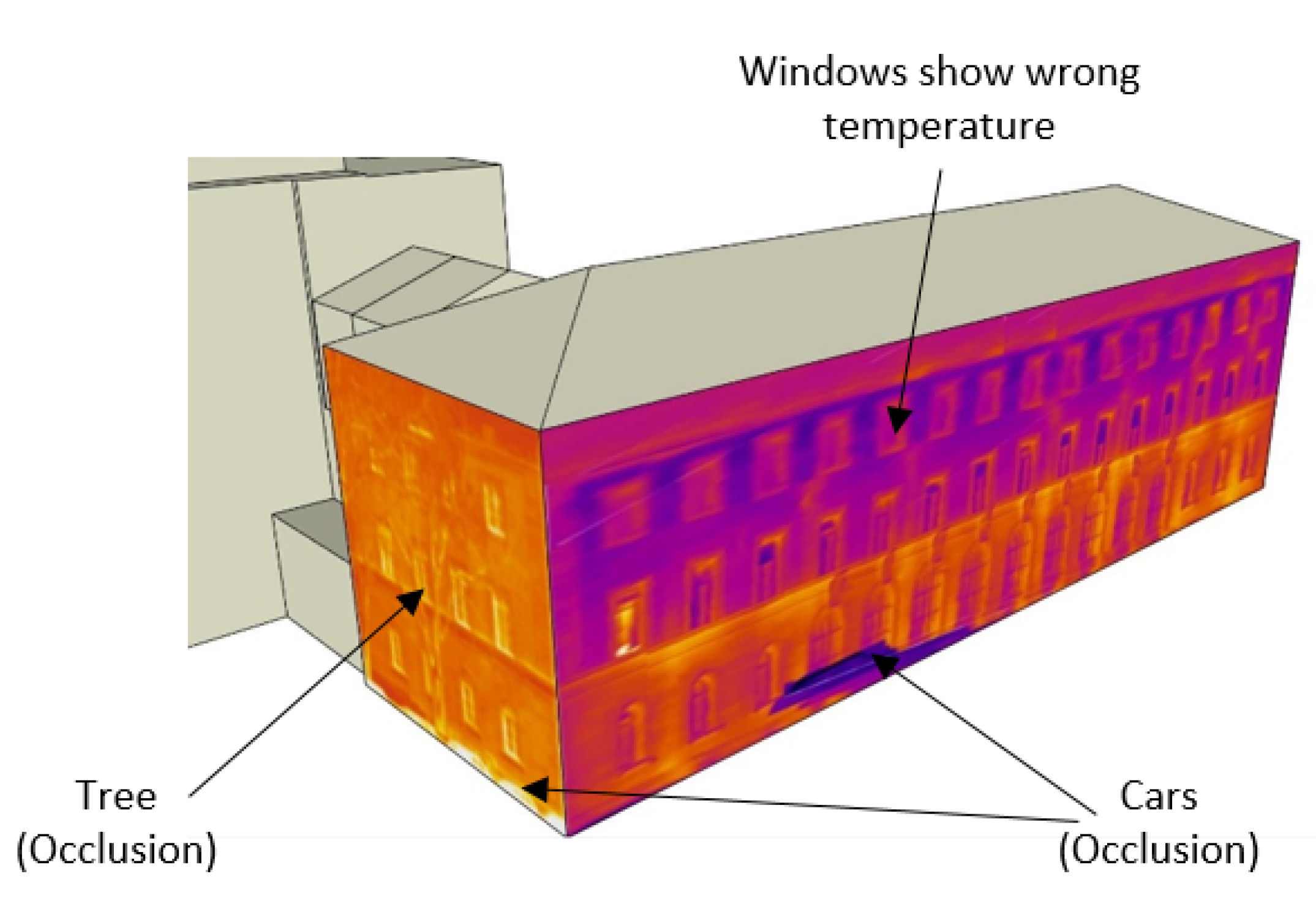Figure 1 shows the facades textured from TIR image sequences based on these approaches. One drawback is that, compared with images in the visual domain, 3D reconstruction of TIR images has less accuracy due to the lower resolution of TIR images. It gives rise to more discretization and decreases matches between the image sequence. Another drawback is that objects in the TIR domain show radiometric behavior, which causes blurred edges and fewer changes in intensity and details in an image. Other drawbacks of the textures extracted using the above-discussed methods are that occlusions are not considered, and they also include window glasses, which often show the wrong temperature due to reflections, as illustrated in Figure 1.

The terrestrial images cannot capture data such as roof structures, inner yards, or backyards. To complement this missing information, oblique images captured from a helicopter or aerial system are necessary. Ref. [25] projects building models into directly georeferenced oblique airborne IR image sequences to perform texture mapping of the building models. Georeferencing, however, is not always precise; in this case, there is no match between the structures in the image and the projected model. Ref. [26] solves this using line-based matching to correct the exterior orientation and determine the best fit between the image sequence and the 3D model.

Contrary to the texture representations, ref. [9] attempted to represent the thermal information in the form of point clouds by preparing thermal point clouds through a combination of TIR image sequences and MLS point clouds. They combined data from various sensors using a data fusion technique. Firstly, they extracted key points from distorted TIR images, then used a restricted Random Sample Consensus (RANSAC)-based algorithm for correspondence determination to estimate the six Degree of Freedom (DOF) pose, and finally fused geometric properties from point clouds and thermal attributes from images using a non-local means strategy. Ref. [27] attempted indoor mapping by adding thermal channels to 3D points by fusing TIR camera images with terrestrial laser scanners and RGB point clouds. They mounted the sensors on a robot platform and calibrated the system geometrically by defining the used coordinate systems and co-registering the laser scanner point cloud and camera images. As the sensors’ field of view differed, they had to synchronize them before fusion. A similar technique for co-registration with a photogrammetric point cloud is shown in [28].

Ref. [29] worked on IR camera calibration to map textures to 3D building models automatically. Texture mapping requires external orientation of images, and direct geo-referencing requires a global positioning system (GPS)/inertial navigation system (INS), which is included in the camera system that was calibrated. They used a helicopter platform to obtain the images. Ref. [30] proposed a technique for texture mapping by finding the best fit between the airborne images and the building model using model-to-image matching. It also extracts texture by selecting the best texture. Ref. [31] assessed the quality of building textures extracted from TIR image sequences from aerial and terrestrial platforms captured using various sensors and orientations. The qualities are compared based on the completeness of texture, viewing angle, the accuracy of the projection, and geometric resolution, to finally select the most accurate and complete textures. Ref. [32] matched IR images with 3D building models for extracting textures. Based on the relative orientation of the point cloud, they matched terrestrial image sequences, and using standardized masked correlation, including system calibration, they also matched airborne images. They introduced the combination of airborne and terrestrial data in a single model. Ref. [33] aligned 3D building models using oblique TIR images captured from a flying platform to extract thermal textures correctly. By establishing correspondences between image line segments and building model edges, they were able to track lines and estimate the optimal camera pose for the best possible match between the image structures and the projected model.

There are some benefits of using point clouds instead of images for texture generation. Images have drawbacks, such as that they include occluded objects and require large overlap between multi-view images. Another drawback is that objects in the TIR domain show radiometric behavior, which causes blurred edges in the generated textures and fewer changes in intensity and details in an image. They also include window glasses, which often show the wrong temperature due to reflections. Projecting or aligning the 3D building models with oblique images requires proper correspondences between the model and structures in the image to estimate the optimal camera pose for the best possible match, which is challenging and also needs accurate georeferencing and an accurate estimation of the external orientation of images. The number of elements visible in the TIR domain influences the position refinement. The refinement quality is greatly reduced in the case of facades with repetitive patterns or few objects. It becomes worse when it happens along with inaccurate GPS positions. The extraction of textures is sensitive to errors in the estimation of viewing direction. To overcome the aforementioned image interpretation challenges in TIR images, we used thermal point clouds. Now, thermal point clouds can also be generated only from TIR images via 3D reconstruction with SfM/the multi-view stereo principle. Still, the reconstruction accuracy will be limited due to the limited geometric density and lower resolution of TIR images that gives rise to more discretization and decreases matches between the image sequence. Homologous points are rarer to find and difficult to locate. Therefore, in this paper, we used point clouds generated with mobile laser scanning that give good location information with usable georeferenced 3D coordinates of buildings, good point density, and accurate geometric details, and then the points were extended with thermal intensities extracted from TIR image sequences. Also, when using point clouds, the occlusions are omitted, as our proposed algorithm selects only the nearest points from the facade for mapping.

3. Methodology

The proposed method for texture generation is embedded into a larger processing chain that uses both MLS point clouds and thermal images to refine existing building models. This paper uses refined LoD3 building models, texture masks, and thermal point clouds as input data for thermal texture generation. For input data preparation, the point cloud and the building model are co-registered and georeferenced wherever necessary, and then the LoD2 building model’s geometry is enriched with facade elements like windows, doors, and underpasses to prepare a refined LoD3 model. These input data are then fed into a thermal mapping algorithm, where we compare different strategies to calculate the thermal intensity values for the texels of the facade texture from the point cloud. The temperature values are projected from the thermal point cloud to the facade using the nearest neighbor algorithm. At first, the building model and point clouds are superimposed over one another. Then, for each texel of the texture layer of the facade, the neighboring points of the point cloud within a certain threshold radius are filtered. The minimum distance point vertical to the texel is selected, and that point’s thermal intensity value is assigned to the texel. This procedure is repeated for all the texels of the texture layer to map the thermal values to the whole facade. After that, a post-processing strategy is applied to the generated texture image. A mask is applied to cut out the windows and doors because the temperature values of windows and doors captured by TIR cameras are inaccurate or distorted due to reflections from glass surfaces. In this way, the TIR textures on the facade are finally established. The overall workflow of the methodology is shown in Figure 2.

3.1. Thermal Mapping Algorithm: Nearest Neighbor Approach

The following points describe the steps implemented in the algorithm:

(i)

Take the texture layer of the facade and consider texels (pixels on texture layer) with a predefined size corresponding to the real world (Ground Sampling Distance (GSD));

(ii)

Take the thermal point cloud and clip it by retaining only points within a threshold distance normal to the facade to decrease the computation time of the nearest neighbor search algorithm and increase efficiency. The point cloud has a resolution layer that contains quality information;

(iii)

For each texel:

(a)

Define neighborhood. Take the neighbor points within a predefined radius;

(b)

Search for the minimum distance point vertical to texel that has a temperature value. The search for the best point can be based on three different approaches: minimizing the angle to normal, minimizing the perpendicular distance to normal, and minimizing only distance;

(c)

Assign the thermal intensity value (weighted by quality layer) of the point to the texel;

(iv)

Repeat the above step 3 until all the temperature values are mapped to the facade.

The mapping method is illustrated graphically in Figure 3.

3.1.1. Clipping the Point Cloud

The thermal point cloud is clipped by retaining points within a predefined threshold distance in front and behind the facade along the normal direction and removing the remaining points. It is necessary to reduce the data size to be processed and to speed up the computation for the nearest neighbor search. The underlying method fits a plane to the 3D point cloud. It sets a threshold distance from the plane to an inlier point and has orientation constraints specified by a 1-by-3 reference vector. The method makes use of M-estimator Sample Consensus (MSAC) [34], which is a variant of the Random Sample Consensus (RANSAC) algorithm, to find the plane. The reference vector is a vector normal to the facade plane and is computed using Singular Value Decomposition (SVD).

3.1.2. Finding the Neighbor Points within a Radius

The neighbor points belonging to the thermal point cloud within a predefined radius from the mid-point of texel are computed using the fast approximate nearest neighbor algorithm provided by [35]. The point cloud is organized in a kd-tree (a generalization of a binary search tree) for optimal neighbor search. After finding the neighbor points, they are stored in an array in a sorted manner (nearest to farthest, based on their Euclidean distances from the texel mid-point) for the next step of the thermal mapping algorithm.

3.1.3. Finding the Nearest Point along Normal Direction to Texel

After filtering the neighbor points in the above step, the task is to select the optimal point whose thermal intensity value can be mapped to the texel. The ideal point would be the closest in the direction exactly normal to the texel surface. In other words, the point should be vertical to the mid-point of the texel. In practice, it is required to search for the point which is closest to the vertical of the texel and also closest to the facade plane. The following sections describe three different approaches for selecting the nearest optimal point.

• Minimize Angle to Normal:

In this approach, we select the nearest optimal point based on the angle to normal. We evaluate the angle between the vector connecting the candidate point to the texel mid-point and the normal vector. Finally, we choose the point where this angle is minimum. (For ideal point vertical to texel, this angle will be zero). The angle is found using the cosine formula (ratio of the dot product of the vectors to the product of the magnitude of the vectors):

$$cos\Theta =\frac{\overrightarrow{N}·\overrightarrow{P_c-P_m}}{\left|\overrightarrow{N}\right|\left|\overrightarrow{P_c-P_m}\right|}$$

(1)

where $\Theta$ is the angle that needs to be minimized, $\overrightarrow{N}$ is the normal vector, and $\overrightarrow{P_c-P_m}$ is the vector from texel mid-point ($P_m$) to the external candidate point ($P_c$) in the point cloud. Figure 4 shows the texel plane (yellow) and the corresponding angles and vectors. For each of the filtered neighbor points, the algorithm checks for the minimum angle points and then selects the closest distance point (from texel mid-point) out of them to map the thermal intensity.

• Minimize Perpendicular Distance to Normal:

In this approach, we select the nearest optimal point based on the perpendicular distance to normal. We calculate the perpendicular 3D distance between the nearby candidate points and the normal vector. Finally, we choose the point with minimum distance. (For the ideal case, this distance should be zero). The perpendicular distance is found using the sine formula:

$$sin\Theta =\frac{\mathrm{perpendicular}}{\mathrm{hypotenuse}}=\frac{D_{\perp }}{\mathrm{distance}\mathrm{between}{P}_c\mathrm{and}{P}_m}$$

(2)

where $D_{\perp }$ is the perpendicular distance from the external candidate point ($P_c$) to the normal vector. It is also shown in Figure 4. For each of the filtered neighbor points, the algorithm checks for the minimum perpendicular distance points and then selects the closest distance point (from texel mid-point) out of them to map the thermal intensity.

• Minimize Only Distance:

In addition to the above two approaches, the third approach is to find only the closest/minimum distance point of the texel’s local neighborhood without considering the normal direction. Here, the algorithm does not consider whether the point is vertical to the texel.

In cases where there is more than one optimal point, the algorithm calculates the median of the thermal intensity and quality values of multiple points for mapping.

The angle-based approach implicitly includes the normal distance of the point to the plane, as the angle depends not only on the absolute distance from the normal to the center point of the texel but also on the distance to the facade plane. It means that if there are two points at the same absolute distance from the normal, but one point is farther away from the facade plane than the other, the farther point will have a smaller angle. It may lead to selecting points far from the facade plane. To avoid such cases, the algorithm checks both the distance and angle, i.e., it tries to minimize the angle and gives preference to closer points simultaneously. On the other hand, this issue is not present in the perpendicular distance-based approach, as it only considers the absolute distance from the normal. All these approaches are implemented, and their results are compared later in this paper.

3.2. Post-Processing

After selecting the nearest optimal point, a resolution layer is applied before mapping the thermal intensity values to the texture layer. The resolution layer contains the quality information of points in the thermal point cloud. The quality corresponds to the distance from the TIR camera (selected image center) to the points. The points at less distance have higher quality or resolution, and vice-versa. The points without thermal attributes are assigned zero values in the quality layer. The windows and doors of the generated texture image are then removed by applying a mask.

4. Experiments

4.1. Test Datasets and Platform Used

The study area is located at the Technical University of Munich (TUM) city campus. We tested on two facades of a three-story building block. The height of the facades is 19 m. The length of one facade is 66 m (surface area 1254 m ${}^2$) and the other is 18 m (surface area 342 m ${}^2$). The total area of the test site is approx. 1400 m ${}^2$ and the volume is 28,000 m ${}^3$. LoD2 building models in CityGML format [36] are used. Point clouds are taken from the TUM-MLS-2016 dataset [37]. Thermal point clouds were provided by [9], who used laser scanner point clouds and TIR image sequences of facades captured from a mobile platform setup Mobile Distributed Situation Awareness (MODISSA) [38]. The MODISSA platform was mounted with sensors: one thermal camera (uncooled microbolometer) Jenoptik IR-TCM 640 (manufactured by Jenoptik AG, Jena, Germany) and two Velodyne HDL-64E LiDAR (Light Detection and Ranging) (manufactured by Velodyne Lidar, San Jose, CA, USA). The Velodyne sensors were mounted on the front roof of a vehicle at 35 degree angles. These sensors were mounted together with a GPS to provide the vehicle’s location information. An Applanix POS LV inertial navigation system was used to georeference the measurements directly. The uncooled thermal camera was mounted crosswise to the driving direction. The thermal camera provided TIR images as 16 bit-TIFFs with lossless compression in the size of 640 pixels × 480 pixels. The LiDAR sensors can record all objects within a 120 m range with up to 2.2 million points per second. Each of the two laser scanners performed more than 8000 scans (rotations of the scanner head) to acquire the point clouds. For more information about the sensors and their specifications, please refer to [38]. The programming and computation were conducted using MATLAB on a computer with 32 GB RAM, a 3.20 GHz CPU, and a 64-bit processor. The 3D building modeling was performed in a Computer-Aided Design (CAD) software, SketchUp. Data integration, transformation, inspection, extraction, and visualization were carried out using the FME platform on a 2.40 GHz CPU (two processors), 32 GB RAM, 64-bit operating system.

4.2. Preparation of Input Data

4.2.1. Pre-Processing and Co-Registering of Input Point Clouds and LoD2 Models

In our study, we carried out manual registration between point clouds and 3D building models. This may seem time- and labor-consuming when compared with automatic registration. But automatic registration can lead to more errors than manual registration. For example, there can be errors in bundle adjustment and also facades may not be properly visible. In contrast, by performing manual registration, we can minimize the errors.

The LoD2 City Geography Markup Language (CityGML) models are georeferenced and reprojected to a standard coordinate system EPSG:25832—ETRS89/Universal Transverse Mercator (UTM) zone 32N. All the input data are transformed into this coordinate system using Feature Manipulation Engine (FME). The point clouds in the local Euclidean coordinate system are georeferenced by performing an affine transformation that includes translations and rotations. The affine transformation is carried out either in FME or MATLAB. If the exact world coordinates are known, then the georeferencing can also be carried out by manually offsetting in the X, Y, and Z directions and 3D rotation. This manual adjustment can always be carried out in FME if there is a mismatch between the transformed and ground truth coordinates.

The point clouds with high volume took a lot of computation time and storage. In FME, point clouds are downsampled to reduce their size. It outputs a point cloud with fewer points than the input and also maintains the original shape. It uses a Medial Axis Transform algorithm to keep more points in areas with high rates of change, while thinning areas with low rates of change. Again, a filter is used in FME to further reduce the size and volume of the point cloud by thresholding with respect to the X, Y, and Z coordinates. Figure 5 shows the transformation of point clouds and building models using the FME workbench.

4.2.2. Establish Refined LoD3 Models and Texture Mask

The LoD2 building model is overlayed with a point cloud. It ensures the exact location of openings like windows and doors. Then, they are modeled using SketchUp. Figure 6 shows the refined building model.

A uniform gray texture is applied to the facade of the refined building model using the 3D modeling software SketchUp, and then the texture mask is extracted without the doors and windows. We will use this gray texture mask later for thermal mapping. These are illustrated in Figure 7.

The thermal point clouds have attributes such as temperature values, quality information, and location coordinates. Figure 8 shows the visibility of the laser scanner and thermal camera in relation to the building model. Figure 8a shows the whole point cloud, while in Figure 8b the points with thermal attributes are colored.

5. Results and Discussion

5.1. Thermal Mapping

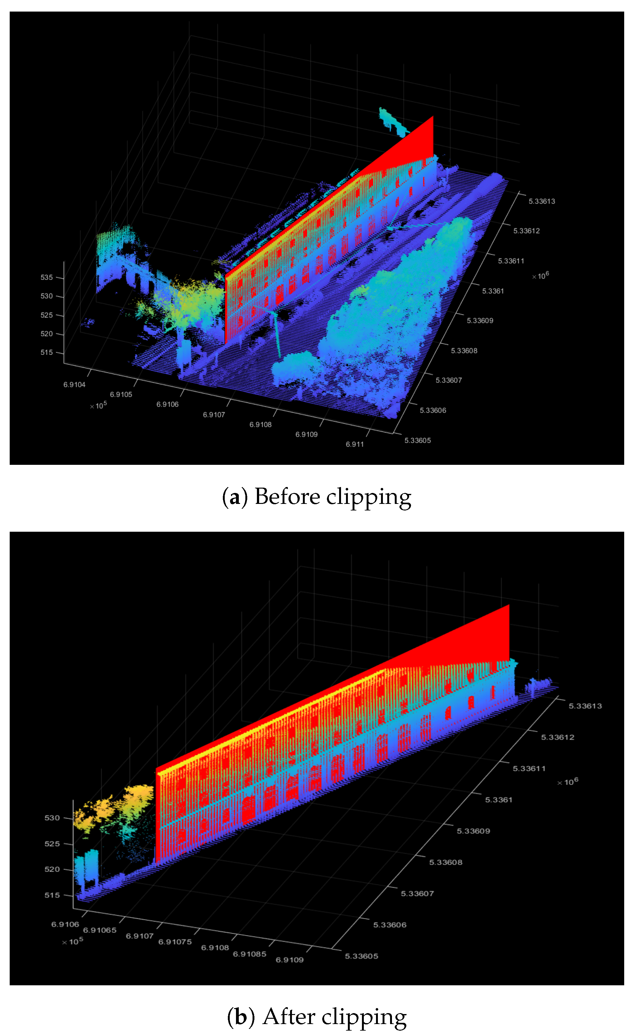
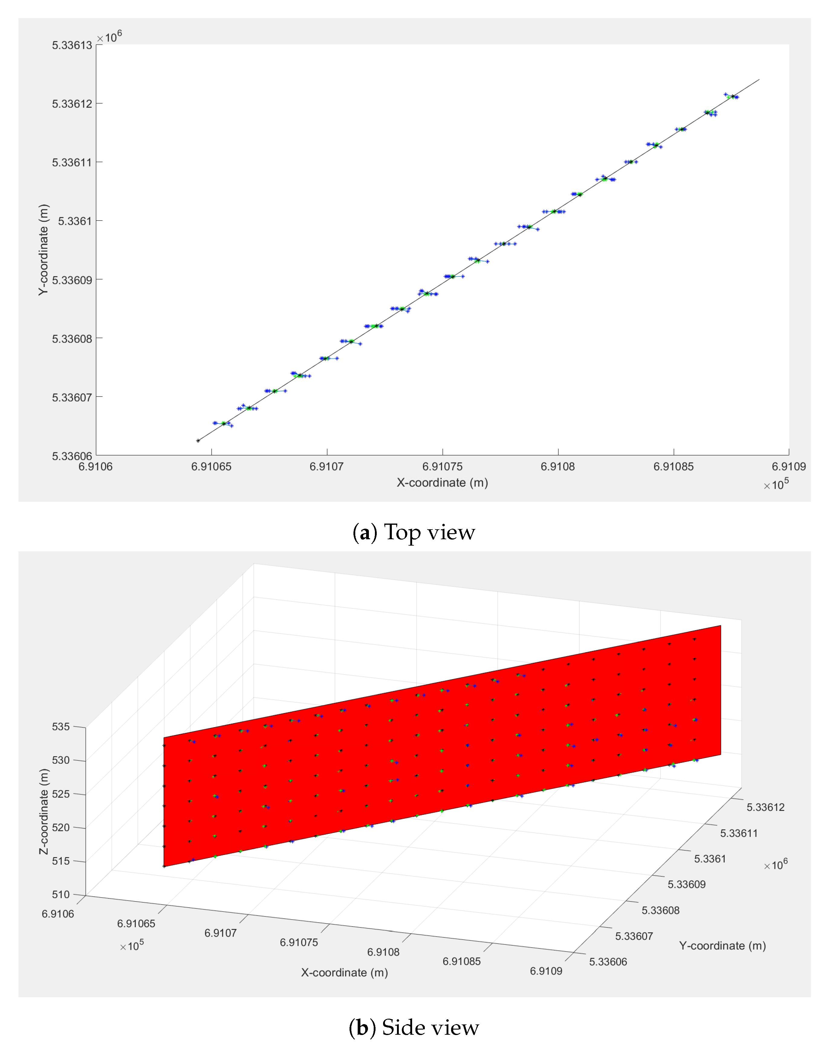
The computation and programming of all the processes discussed in this section were performed in MATLAB. The texture layer of one facade is taken with the texel size set to 10 cm × 10 cm corresponding to the real world (i.e., 10 cm GSD). The thermal point cloud is taken and then clipped to contain only points within a threshold 1 m in front and behind the facade, in the normal direction. As mentioned before, this reduces the computation time of the nearest neighbor search algorithm. Figure 9 shows the point cloud before and after clipping, together with the facade plane. The facade is shown in red color and the point clouds in blue/yellow/green colors. From the figure, it can be seen that only the closest and relevant points within 1 m normal to the facade are retained after clipping.

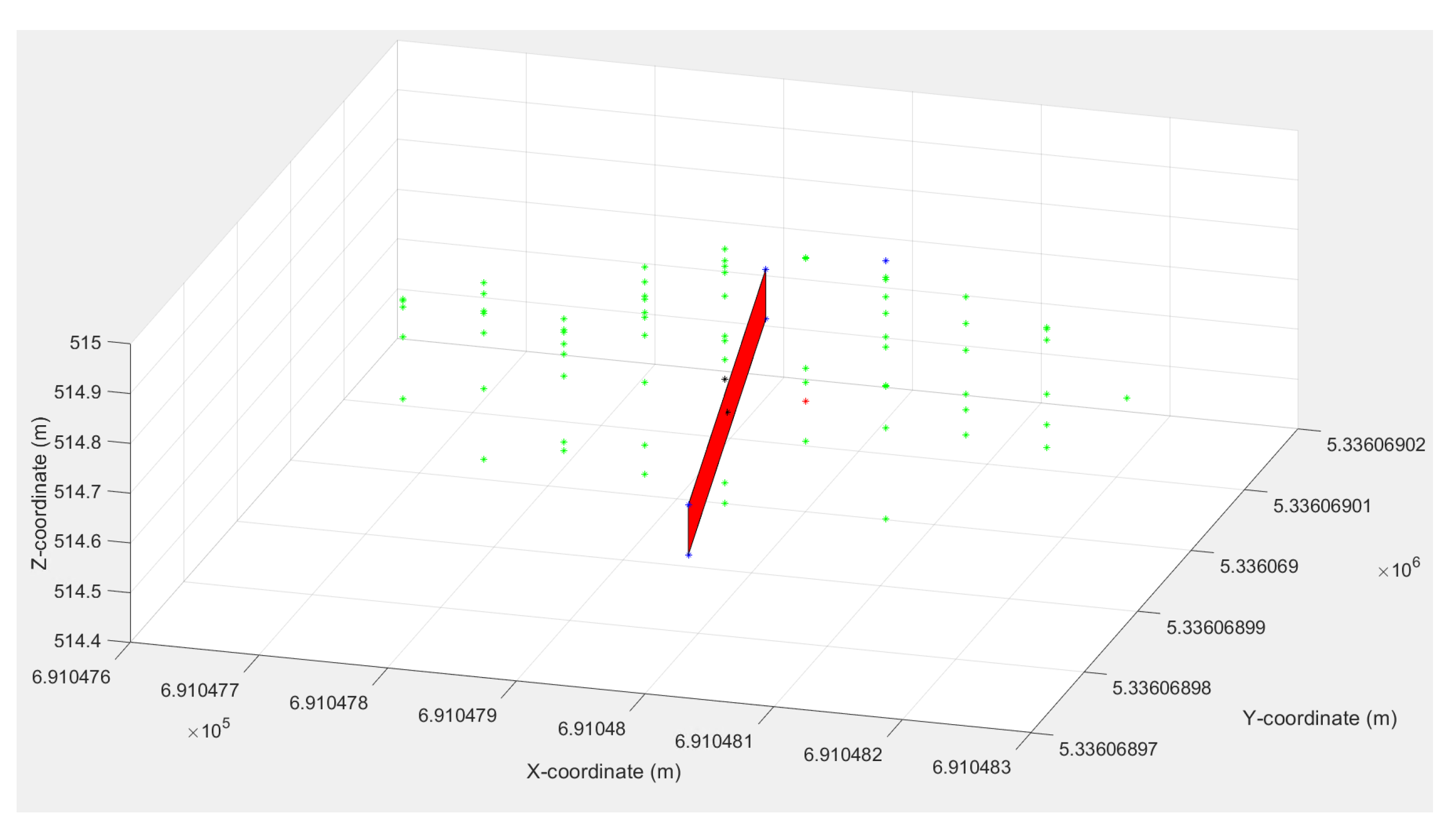
The next step is to define the neighborhood for each texel, i.e., to find neighbor points in the thermal point cloud within a predefined radius from the mid-point of the texel. The radius is set to 1 m. Later, in Section 5.3, it will be discussed how the performance is affected when we change the radius from 0.3 m to 1 m. Figure 10 shows the neighbor points (green) for a single texel plane (red).

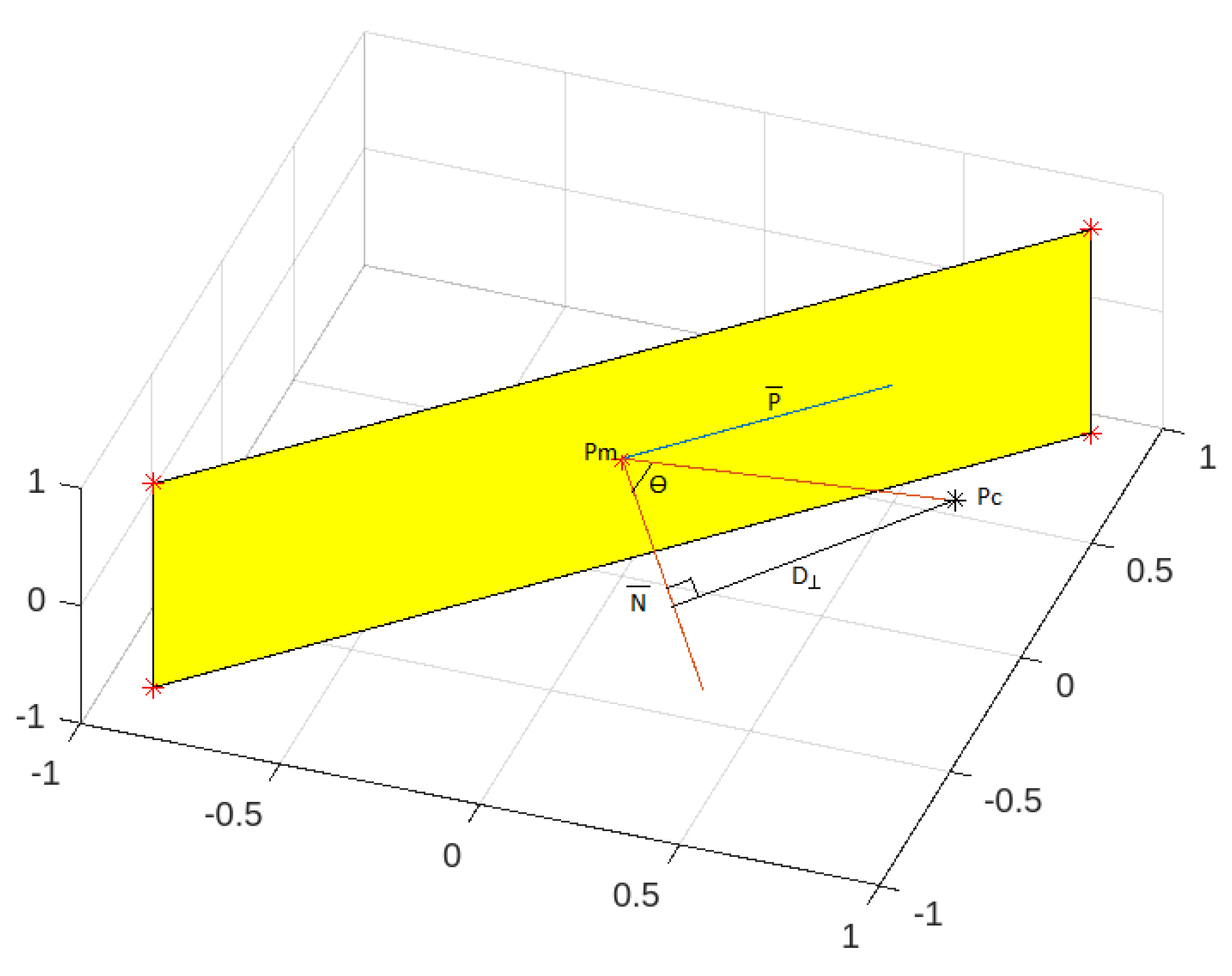
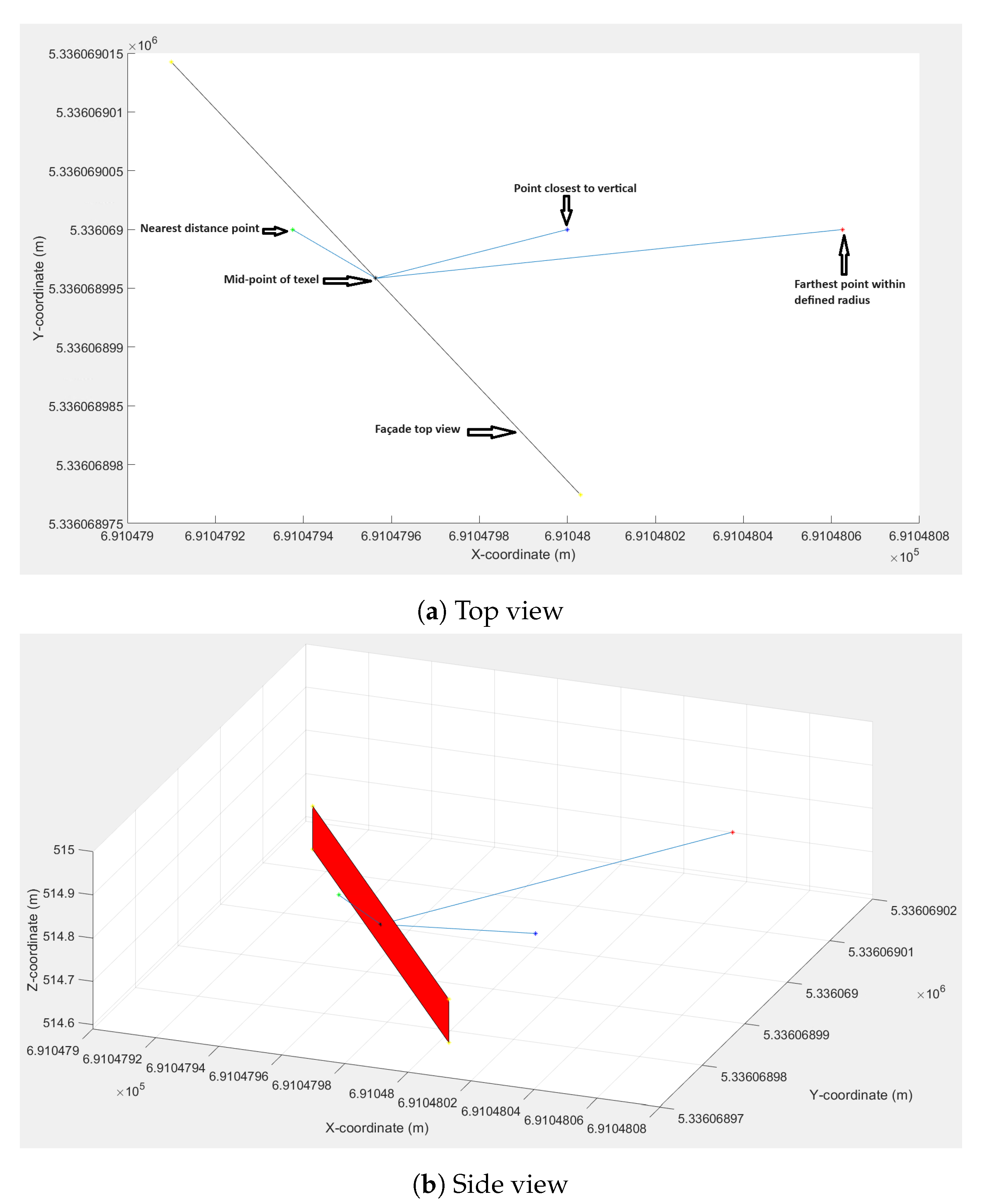
Then, the algorithm searches for the nearest point vertical to the texel and which has a temperature attribute. Three methods are approached: angle to normal vector, perpendicular distance to normal vector, and distance without considering their verticality. We already discussed these three approaches in detail in the previous section. Their performance results will be discussed and compared later in Section 5.2. Figure 11 shows the detected optimal point closest to the vertical (blue) for a single texel plane (red), the nearest distance point (green), the farthest point within a predefined radius (red), and lines connecting the texel mid-point (black) to the detected points for illustration. The figure shows both the top view and side view. From the figure, it can be clearly seen that the nearest distance point is not normal to the texel mid-point, and the point closest to vertical is a bit far from the nearest distance point.

For illustration, Figure 12 shows how the detected points look for the whole facade plane (red), considering texels at a distance 3 m apart from each other and skipping all the other texels in between them. It can be clearly seen from the figure that some detected optimal points (blue) are behind the facade. This is obvious because the mapping algorithm searches for points on both sides of the facade.

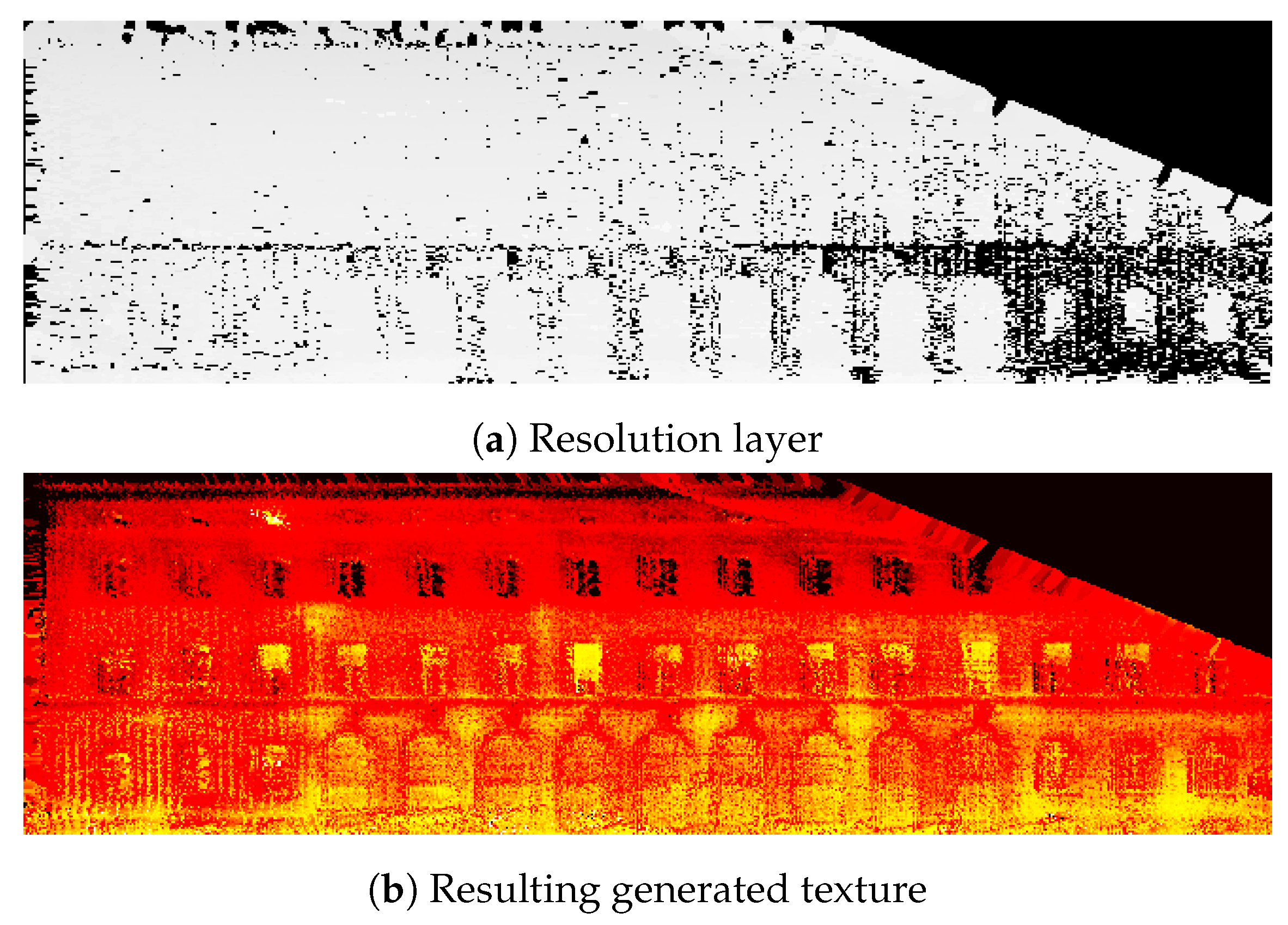
After finding the optimal point, the thermal attribute of that point, weighted by the resolution layer, is mapped to the texel. Figure 13a shows the resolution layer applied to the texels, with the brighter pixels having better quality and darker pixels showing worse quality. From the figure, it is clear that all the points are not of the same quality and, especially, more points on the right side are bad quality. Therefore, it makes complete sense to weight the thermal intensities with quality information before mapping. The upper right corner has completely black pixels, as it does not have thermal attributes. And this is evident when we look at the input point clouds in Figure 8, as they have no points in this corner region. The mapped thermal texture is a low-light image that is brightened and a heat map is applied as a color map to visualize the temperature distribution better. Figure 13b shows the resulting generated texture. In the texture, we can see some heating pipes in the shape of cylinders; thermal lintels, bridges, and anomalies in the shape of blobs (near windows/doors).

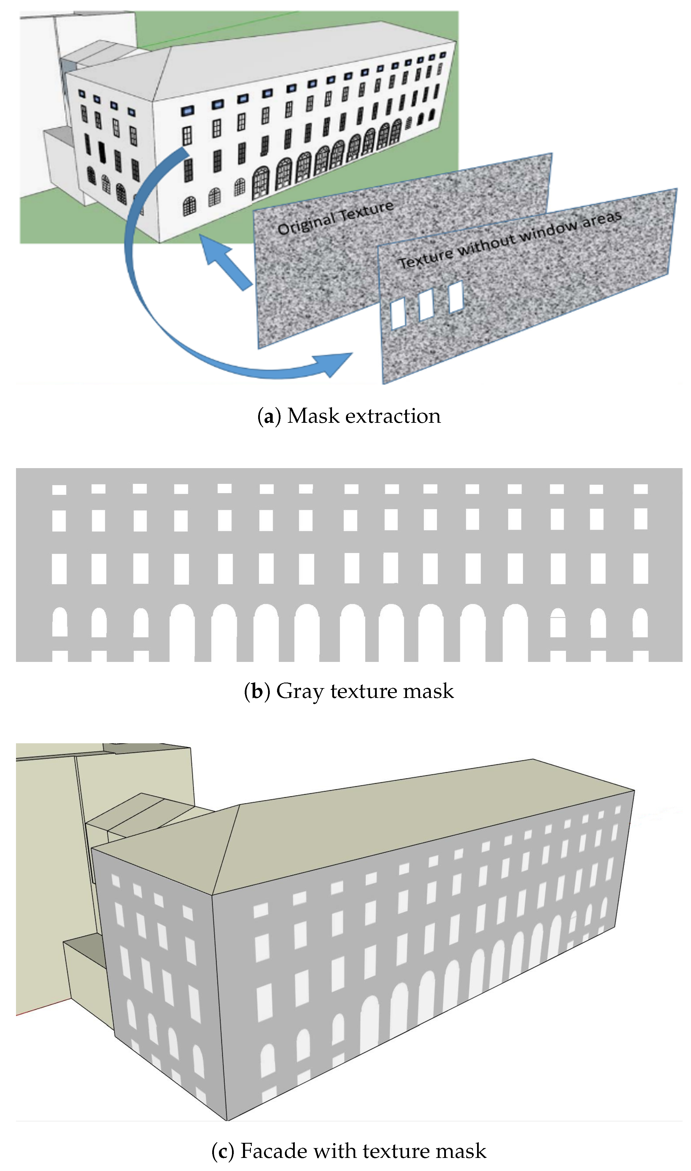
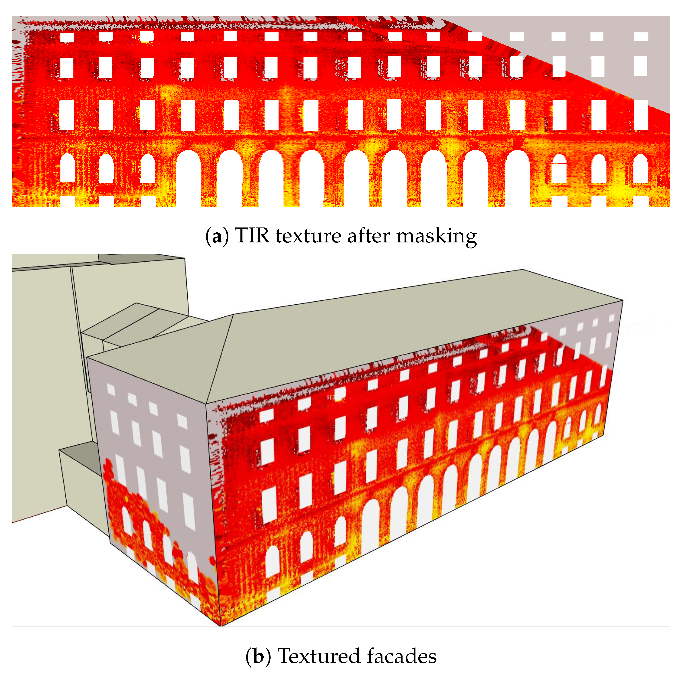
Finally, the extracted gray texture mask, shown in Figure 7b, is applied to remove the doors and windows and to assign a uniform gray value to the texels where no thermal intensity is mapped. The mask is binarized via thresholding and blended with the texture in Figure 13b to generate the final TIR texture, as shown in Figure 14a. It is implemented on two facades, as shown in Figure 14b.

The source thermal point cloud shown in Figure 8b and the resulting textured facade in Figure 14b look quite consistent. Therefore, this proves that the projection algorithm works quite well. Also, in comparison, Figure 14b clearly shows that the occlusions are not mapped, as the algorithm selects the nearest points from the facade for mapping, unlike in the case in Figure 1. Additionally, the windows are excluded by using texture masks. Therefore, our method shows an advantage over the previous approach.

5.2. Comparison of Different Approaches for Searching Nearest Point

Earlier, we discussed three different approaches for searching for the nearest point. In this section, we will compare their performance results. The purpose of this analysis is to find out the best-suited approach that yields the best texture resolution at the best computation cost. The first approach minimizes the angle between the vector normal to the texel and the vector connecting the optimal candidate point to the texel mid-point. The second approach minimizes the 3D perpendicular distance between the optimal candidate point and the normal vector. The third approach is to select only the minimum distance point with a temperature value without considering if it is vertical to the texel or not. The second approach yielded the finest pixels.

Table 1. Detection results based on different approaches for searching the nearest optimal point. There are a total of 126,060 texels, out of which 114,446 could be assigned a TIR value.

Parameters	Minimize Angle to Normal	Minimize Perpendicular Distance to Normal	Minimize Only Distance
Texels with optimal point farther than nearest point	113,792	103,083	13,444
Texels with multiple optimal points	1130	7177	0
Mean distance from optimal points to texels	0.4597 m	0.4597 m	0.1736 m
Mean angle to normal vector	7.19°	7.42°	82.48°
Mean perpendicular distance to normal vector	0.0575 m	0.0413 m	0.1721 m
Window/door texels	23,342	23,342	23,342
Texels with thermal attributes (without windows/doors)	91,104	91,104	91,104
Processing time	177 min	186 min	23 min

shows the detection results based on the three approaches for one facade.

The computation time is apparently much more for the first two approaches because it has to complete the extra computation to find the point closest to vertical. On the other hand, the third approach is quite fast, as it only searches for the nearest point. Also, it has the least mean distance from the optimal points to texels, which is quite apparent. As it does not consider verticality, it has a high mean angle and high mean perpendicular distance to the normal vector. The mean angle to normal for the first approach is 7.19°, which is very close to normal and looks good. For the second approach, the mean perpendicular distance to normal is 0.0413 m, which is also close to vertical and is quite satisfactory. Considering the above factors, there is a trade-off between the texture resolution and computation time. The second approach yields the finest texture, but at the cost of processing time (186 min), while the third approach generates the coarsest texture, but is quite fast (23 min). Therefore, the user can choose one of these approaches based on their needs and priorities.

5.3. Tuning the Radius to Find Neighbor Points of the Texel

As mentioned earlier, to define the neighborhood of the texel, we need to set a predefined radius. The radius signifies the search space for the nearest neighbor. The larger the radius, the more the search space, and vice versa. The selection of an optimal search space is crucial for the thermal mapping algorithm. Therefore, the purpose of this analysis is to find out the deciding factors for an optimal search space. The mapping results are affected by changing the radius, which is discussed in this section. We want to analyze what is the best-fitting radius that yields a good detection rate and a good quality texture in a reasonable processing time.

Table 2. Detection results based on changing radius of neighborhood.

Parameters	Radius = 0.3 m	Radius = 0.5 m	Radius = 0.7 m	Radius = 1 m
Detection rate	83.93%	87.15%	88.97%	90.78%
Detection rate (without windows/doors)	80.28%	84.23%	86.47%	88.69%
Processing time	15 min	44 min	89 min	191 min
Mean distance from optimal points to texels	0.1928 m	0.2448 m	0.2854 m	0.3377 m
Mean perpendicular distance to normal vector	0.0926 m	0.0807 m	0.0783 m	0.0818 m

shows the results for one facade.

The detection rate signifies the proportion of texels for which a corresponding temperature value can be detected and mapped. With an increasing radius, this rate increases, which seems logical because the search space increases as more neighbor points are considered. The computation time also increases as more points need to be processed. The mean distance from the optimal points to texels increases, which is also obvious because more points imply more outliers. The mean perpendicular distance to the normal vector is approximately 0.08 m, which is close to vertical. Therefore, it looks like the deciding factors are the detection rate and computation time. Changing the radius from 0.3 m to 0.5 m increases the detection rate significantly. It can also be seen in the generated textures, whose quality improves (becomes finer) and has fewer texels with no thermal intensity. But the computation time also increases three-fold. Changing the radius further to 0.7 m or 1 m does not improve the detection rate much, but the processing time keeps increasing significantly. Therefore, looking at these factors, a radius of 0.5 m seems to be a good trade-off where one can assure good quality in a reasonable processing time. Moreover, the best dimensions of the neighborhood will also depend on the texel size and point cloud density. If the GSD is reduced, fewer neighbor points will be available for each texel and, therefore, need a larger radius to include more points. Similarly, more points are available per texel for a higher point cloud density, so a lower radius would suffice. Nevertheless, reducing the GSD and increasing the point cloud density will definitely require more computation cost and time. Therefore, considering these factors, an automated method to deduce the best-fitting dimensions of the neighborhood will be quite useful.

5.4. Bilinear Interpolation

As an additional experiment, we computed the texel intensity using bilinear interpolation. To validate our choice of the nearest neighbor approach, we compared it with bilinear interpolation. Later, in Section 5.5, we perform an accuracy analysis of these two methods and show that the nearest neighbor approach outperforms the bilinear interpolation.

For bilinear interpolation, we project each point in the point cloud normally to a facade plane. Then, we take the interpolated value of four projected neighbor points for each texel. The bilinear texture mapping process can be described by the following steps:

(i)

Filter and take planar points from the point cloud. Fit a plane to the thermal point cloud with a maximum allowable distance of 0.5 m from the facade. Retain all the inlier points in the plane and discard the remaining points in the point cloud. We used the M-estimator SAmple Consensus (MSAC) algorithm to find the plane. Figure 9b shows the planar points.

(ii)

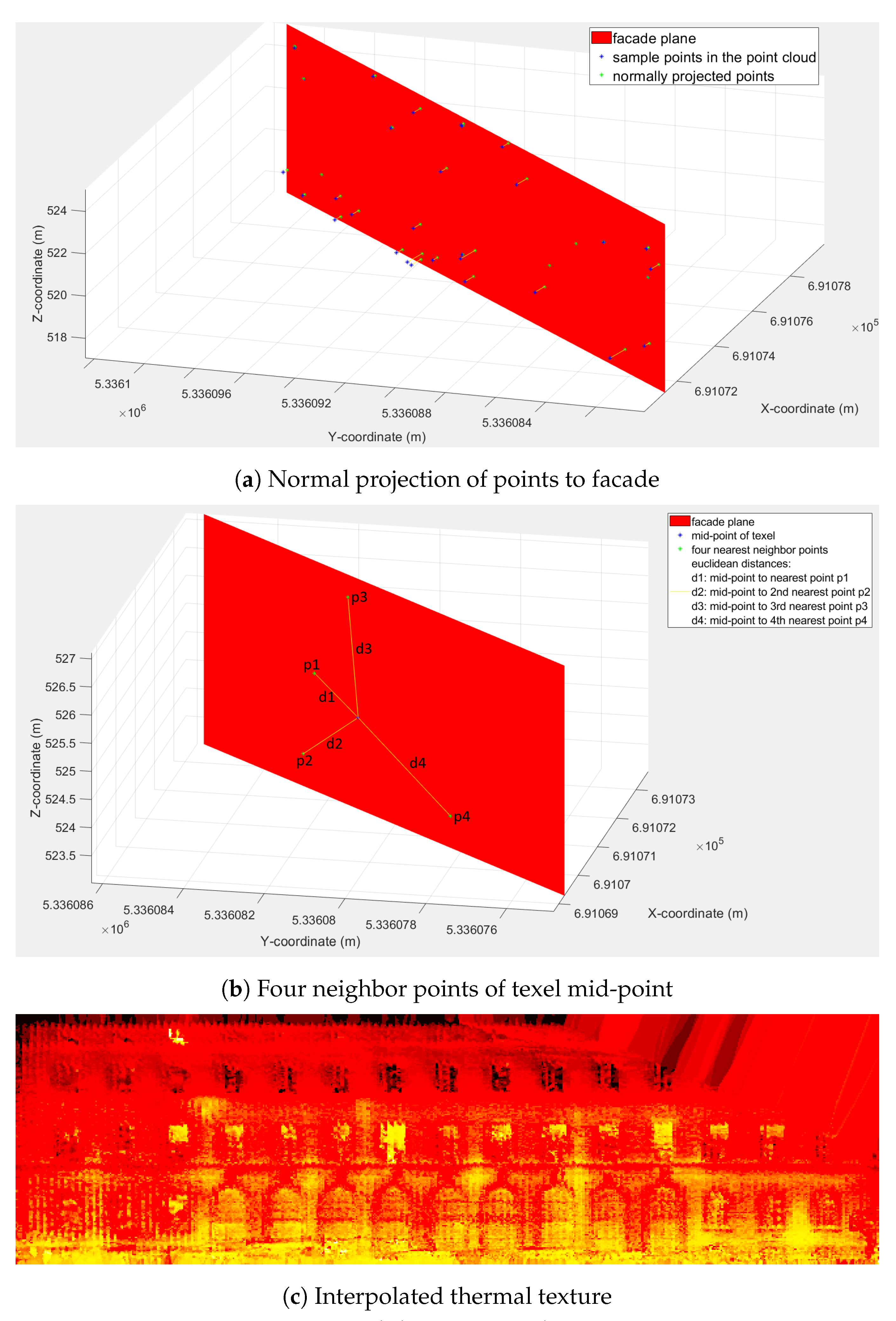
Project each point in the plane normally to the facade. We only projected the points with a temperature value. Therefore, the points with no thermal attributes are discarded. Figure 15a shows some sample points (blue) from the point cloud projected normally to the facade plane. The points after the projection are depicted in green.

(iii)

Take the texture layer of the facade (with the same GSD 10 cm). We take the mid-point of each texel and find its four nearest neighbor points from the above-projected points. The nearest neighbors are found by using the Kd-tree-based search algorithm. In Figure 15b, we show the mid-point of the texel in blue, the four nearest neighbor points ($p1,p2,p3,p4$) in green, and the corresponding Euclidean distances ($d1,d2,d3,d4$) between the mid-point and the neighbor points in yellow.

(iv)

Finally, for each texel, we perform bilinear interpolation of the thermal attributes of the four neighbor points.The interpolated value is based on a weighted mean, with the highest weight given to the lowest distance point and vice versa. The interpolated value is calculated as:

$$\begin{gathered} \begin{array}{c}{V}_{interpolate}=(w1\times v1)+(w2\times v2)+(w3\times v3)+(w4\times v4);\end{array} \\ w1={\displaystyle \frac{d4}{d1+d2+d3+d4}}, \\ w2={\displaystyle \frac{d3}{d1+d2+d3+d4}}, \\ w3={\displaystyle \frac{d2}{d1+d2+d3+d4}}, \\ w4={\displaystyle \frac{d1}{d1+d2+d3+d4}}; \end{gathered}$$

(3)

where $w1,w2,w3,andw4$ are the weights and $v1,v2,v3,$ and $v4$ are the temperature values (weighted by the resolution layer) corresponding to the neighbor points $p1,p2,p3,$ and $p4$. The highest weight, $w1$, corresponds to the nearest point, $p1$, and the lowest weight, $w4$, corresponds to the farthest point, $p4$. Therefore, $d1<d2<d3<d4\Rightarrow w4<w3<w2<w1$.

The interpolated thermal value is finally assigned to the mid-point of the texel. We repeated this step for all texels until all the interpolated values were mapped to the facade.

Figure 15c shows the thermal texture generated by bilinear interpolation. The interpolation changed the original temperature values and generated some intermediate average values, so all the texels in the generated texture image are assigned a value and there are no blank texels. Therefore, we can see that the upper right corner is also filled up with some interpolated values, even though there are no corresponding points in that region in the input thermal point cloud (Figure 8).

5.5. Performance Evaluation

In our study, we registered point clouds with 3D building models. The registration may cause some errors, such as shift and tilted point clouds. This can lead to incorrect projection directions and can impact the mapping results. For example, the mapped temperature intensity of a point may shift from its original location. Therefore, it is necessary to evaluate the mapping accuracy. The purpose of this analysis is to evaluate and compare the mapping accuracy of our proposed method and some similar/former methods.

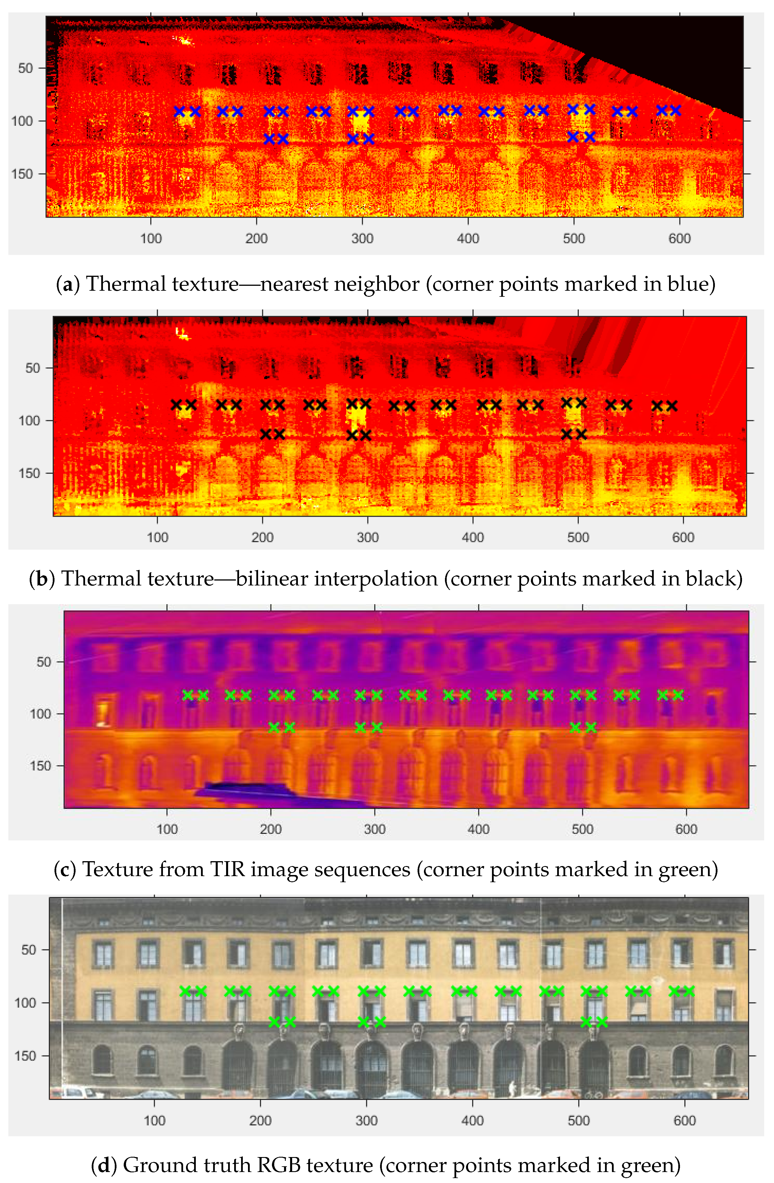
The accuracy or correctness of the texture is evaluated based on the window’s corner points. We manually selected some corner points which were distinctly visible in the thermal texture. We calculated the deviation/shift of these points from a ground truth RGB texture of the facade. From the discussion in previous sections, the approach “Minimize perpendicular distance to normal” for searching the nearest point yields the finest texture, and a radius of 0.5 m seems to be a good trade-off to obtain good quality at a higher detection rate. Therefore, we took these as a use case for calculating the performance metrics. Figure 16a shows the window corner points (blue) in the thermal texture and Figure 16d shows the ground truth RGB texture (corners marked in green).

For deviation, we calculated the Euclidean distance between the pixel coordinates of the generated thermal texture and the ground truth RGB texture. Finally, we evaluated the root-mean-square deviation (RMSD) of our nearest neighbor approach as follows:

$$RMS{D}_{NN}=\sqrt{\frac{{\sum }_{i=1}^N\left\{{(x_{ti}-x_{gi})}^2+{(y_{ti}-y_{gi})}^2\right\}}{N}}$$

(4)

where $x_t$ and $y_t$ are the corner point coordinates of thermal texture (nearest neighbor), $x_g$ and $y_g$ are the corner point coordinates of ground truth RGB texture, and N is the total number of corner points.

We obtained an $RMS{D}_{NN}$ value of 0.7 m, which seems satisfactory. For perfect results, this value should tend to zero.

To further strengthen the accuracy analysis of our proposed method, we will compare our study’s results with similar/former studies. As a use case for similar study, we take the thermal texture generated using bilinear interpolation (shown in Figure 16b, corners marked in black color) and calculate its deviation from the ground truth RGB texture. The RMSD value for bilinear interpolation is calculated as:

$$RMS{D}_{BI}=\sqrt{\frac{{\sum }_{i=1}^N\left\{{(x_{bi}-x_{gi})}^2+{(y_{bi}-y_{gi})}^2\right\}}{N}}$$

(5)

where $x_b$ and $y_b$ are the corner point coordinates of thermal texture (bilinear interpolation).

The estimated $RMS{D}_{BI}$ value is 1.6 m, which is more than the value for nearest neighbor. This proves that the nearest neighbor has better accuracy than bilinear interpolation.

As a use case for previous studies, we take the texture generated from a sequence of thermal infrared images [6,24]. This is shown in Figure 16c (corners marked in green). Similarly, we calculate its deviation from the ground truth RGB texture. The RMSD value for the image texture is defined as:

$$RMS{D}_{IM}=\sqrt{\frac{{\sum }_{i=1}^N\left\{{(x_{mi}-x_{gi})}^2+{(y_{mi}-y_{gi})}^2\right\}}{N}}$$

(6)

where $x_m$ and $y_m$ are the corner point coordinates of the texture from TIR image sequences.

The $RMS{D}_{IM}$ value is estimated to be 1.37 m, which is again more than the value for nearest neighbor. This shows that the nearest neighbor also has better accuracy than the texture generated from TIR image sequences.

Therefore, from the accuracy point of view, our proposed nearest neighbor method outperformed both bilinear interpolation and texture from image sequences ($RMS{D}_{NN}<RMS{D}_{IM}<RMS{D}_{BI}$).

Therefore, the performance evaluation supported our choice of the nearest neighbor approach over bilinear interpolation. Earlier, we mentioned that texture generation from TIR images can lead to projection errors due to the limited level of detail of building models. We verified that since our nearest neighbor method is better in terms of accuracy ($RMS{D}_{NN}<RMS{D}_{IM}$). Our approach does not map occlusions, which is evident in Figure 1 and Figure 13b. Therefore, our results verify our contributions and the gaps we fill in the literature.

6. Conclusions

This paper proposes a framework to map temperature attributes from thermal point clouds to building facades to prepare a thermal 3D description of buildings. The goal is to enrich building models with thermal textures. The texture layer of the facade and point clouds are fed into a thermal mapping algorithm that uses a nearest-neighbor approach to find an optimal point closest to vertical within a predefined neighborhood of points. The thermal intensity of the optimal point is read, weighted by a resolution layer, and then assigned to texels. The mapped thermal texture is further enhanced through post-processing stages to generate the final TIR texture that is applied to the facade. Instead of interpolation, the nearest neighbor method is selected because it retains the original temperature values. Three different approaches for searching the nearest point are attempted: “Minimize angle to normal”, “Minimize perpendicular distance to normal”, and “Minimize only distance”. The approach “Minimize perpendicular distance to normal” yields the finest texture resolution at a reasonable processing time. This approach yielded a 0.0413 m mean perpendicular distance to normal, which is close to vertical and is quite satisfactory. The radius of the neighborhood that signifies the search space is tuned. A radius of 0.5 m provides a good trade-off of better quality and a higher detection rate at a reasonable computation cost. The accuracy of the generated texture is evaluated based on the shift in the window corner points from a ground truth RGB texture. The deviation/shift is calculated using a performance metric, RMSD, and its value for our nearest neighbor method is found to be 0.7 m, which is satisfactory. In terms of accuracy, the nearest neighbor method is compared with bilinear interpolation and an existing TIR image-based texturing method. The RMSD value of the nearest neighbor method is found to be the lowest, which implies that it has better accuracy than the other two methods. Our approach is compared with existing texturing methods and is found to have some advantages, such as occlusions being removed and windows that show the wrong temperature being excluded. Some benefits of using point clouds instead of TIR images are discussed. Texture generation directly from TIR images can lead to projection errors due to simplified building models. That is why texture is generated by projecting point clouds. The limited geometric density and accuracy of TIR images can lead to poor 3D reconstruction. That is why laserscanner point clouds extended with thermal intensities are used in our method instead of 3D reconstructed point clouds. The current implementation of our method is carried out on an outdoor facade. In the future, we aim to include indoor thermal mapping, thermal pattern analysis, processing time optimization, and performance evaluation with a manually generated annotated model.

References

1. Balaras, C.A.; Argiriou, A. Infrared thermography for building diagnostics. Energy Build. 2002, 34, 171–183. [Google Scholar] [CrossRef]
2. Garrido, I.; Lagüela, S.; Arias, P.; Balado, J. Thermal-based analysis for the automatic detection and characterization of thermal bridges in buildings. Energy Build. 2018, 158, 1358–1367. [Google Scholar] [CrossRef]
3. Krawczyk, J.; Mazur, A.M.; Sasin, T.; Stokłosa, A. Infrared building inspection with unmanned aerial vehicles. Prace Instytutu Lotnictwa 2015, 240, 32–48. [Google Scholar] [CrossRef]
4. Lerma, J.L.; Cabrelles, M.; Portalés, C. Multitemporal thermal analysis to detect moisture on a building façade. Constr. Build. Mater. 2011, 25, 2190–2197. [Google Scholar] [CrossRef]
5. Rakha, T.; Gorodetsky, A. Review of Unmanned Aerial System (UAS) applications in the built environment: Towards automated building inspection procedures using drones. Autom. Constr. 2018, 93, 252–264. [Google Scholar] [CrossRef]
6. Hoegner, L.; Stilla, U. Mobile thermal mapping for matching of infrared images with 3D building models and 3D point clouds. Quant. InfraRed Thermogr. J. (QIRT) 2018, 15, 252–270. [Google Scholar] [CrossRef]
7. Ham, Y.; Golparvar-Fard, M. Mapping actual thermal properties to building elements in gbXML-based BIM for reliable building energy performance modeling. Autom. Constr. 2015, 49, 214–224. [Google Scholar] [CrossRef]
8. Golparvar-Fard, M.; Ham, Y. Automated diagnostics and visualization of potential energy performance problems in existing buildings using energy performance augmented reality models. J. Comput. Civ. Eng. 2014, 28, 17–29. [Google Scholar] [CrossRef]
9. Zhu, J.; Xu, Y.; Ye, Z.; Hoegner, L.; Stilla, U. Fusion of urban 3D point clouds with thermal attributes using MLS data and TIR image sequences. Infrared Phys. Technol. 2021, 113, 103622. [Google Scholar] [CrossRef]
10. Wang, C.; Cho, Y.K.; Gai, M. As-is 3D thermal modeling for existing building envelopes using a hybrid LIDAR system. J. Comput. Civ. Eng. 2013, 27, 645–656. [Google Scholar] [CrossRef]
11. Westfeld, P.; Mader, D.; Maas, H.G. Generation of TIR-attributed 3D point clouds from UAV-based thermal imagery. In Photogrammetrie-Fernerkundung-Geoinformation; Schweizerbart’sche Verlagsbuchhandlung: Stuttgart, Germany, 2015; pp. 381–393. [Google Scholar]
12. Lagüela, S.; Armesto, J.; Arias, P.; Zakhor, A. Automatic procedure for the registration of thermographic images with point clouds. In Proceedings of the XXII Congress of the International Society for Photogrammetry and Remote Sensing, Melbourne, Australia, 25 August–1 September 2012. [Google Scholar]
13. Maset, E.; Fusiello, A.; Crosilla, F.; Toldo, R.; Zorzetto, D. Photogrammetric 3D building reconstruction from thermal images. ISPRS Ann. Photogramm. Remote Sens. Spat. Inf. Sci. 2017, 4, 25. [Google Scholar] [CrossRef]
14. Yamaguchi, M.; Truong, T.P.; Mori, S.; Nozick, V.; Saito, H.; Yachida, S.; Sato, H. Superimposing thermal-infrared data on 3D structure reconstructed by RGB visual odometry. IEICE Trans. Inf. Syst. 2018, 101, 1296–1307. [Google Scholar] [CrossRef]
15. Yang, M.D.; Su, T.C.; Lin, H.Y. Fusion of infrared thermal image and visible image for 3D thermal model reconstruction using smartphone sensors. Sensors 2018, 18, 2003. [Google Scholar] [CrossRef] [PubMed]
16. Alba, M.I.; Barazzetti, L.; Scaioni, M.; Rosina, E.; Previtali, M. Mapping infrared data on terrestrial laser scanning 3D models of buildings. Remote Sens. 2011, 3, 1847–1870. [Google Scholar] [CrossRef]
17. Scaioni, M.; Rosina, E.; Barazzetti, L.; Previtali, M.; Redaelli, V. High-resolution texturing of building facades with thermal images. Proc. SPIE 2012, 8354, 14. [Google Scholar] [CrossRef]
18. Borrmann, D.; Elseberg, J.; Nüchter, A. Thermal 3D mapping of building façades. In Intelligent Autonomous Systems 12; Springer: Berlin/Heidelberg, Germany, 2013; pp. 173–182. [Google Scholar]
19. Dahaghin, M.; Samadzadegan, F.; Javan, F.D. 3D thermal mapping of building roofs based on fusion of thermal and visible point clouds in uav imagery. Int. Arch. Photogramm. Remote Sens. Spat. Inf. Sci. 2019, 42, 271–277. [Google Scholar] [CrossRef]
20. Lin, D.; Jarzabek-Rychard, M.; Tong, X.; Maas, H.G. Fusion of thermal imagery with point clouds for building façade thermal attribute mapping. ISPRS J. Photogramm. Remote Sens. 2019, 151, 162–175. [Google Scholar] [CrossRef]
21. Hoegner, L.; Stilla, U. Building facade object detection from terrestrial thermal infrared image sequences combining different views. ISPRS Ann. Photogramm. Remote Sens. Spat. Inf. Sci. 2015, 2, 55–62. [Google Scholar] [CrossRef]
22. Hoegner, L.; Stilla, U. Automatic generation of façade textures from terrestrial thermal infrared image sequences. In Proceedings of the 12th Quantitative InfraRed Thermography Conference, France, Bordeaux, 7–11 July 2014. [Google Scholar]
23. Hoegner, L.; Kumke, H.; Meng, L.; Stilla, U. Automatic extraction of textures from infrared image sequences and database integration for 3D building models. In PFG Photogrammetrie-Fernerkundung-Geoinformation; Schweizerbart’sche Verlagsbuchhandlung: Stuttgart, Germany, 2007; pp. 459–468. [Google Scholar]
24. Hoegner, L.; Stilla, U. Automated Generation of Building Textures from Infrared Image Sequences. Int. Arch. Photogramm. Remote Sens. Spat. Inf. Sci. 2007, 36, 65–70. [Google Scholar]
25. Stilla, U.; Kolecki, J.; Hoegner, L. Texture mapping of 3D building models with oblique direct geo-referenced airborne IR image sequences. In Proceedings of the ISPRS Hannover Workshop, Hannover, Germany, 2–5 June 2009. [Google Scholar]
26. Iwaszczuk, D.; Hoegner, L.; Schmitt, M.; Stilla, U. Line based matching of uncertain 3d building models with ir image sequences for precise texture extraction. In Photogrammetrie-Fernerkundung-Geoinformation; Schweizerbart’sche Verlagsbuchhandlung: Stuttgart, Germany, 2012; pp. 511–521. [Google Scholar]
27. Hoegner, L.; Abmayr, T.; Tosic, D.; Turzer, S.; Stilla, U. Fusion of TLS and RGB point clouds with TIR images for indoor mobile mapping. In Proceedings of the 14th Quantitative InfraRed Thermography Conference (QIRT 2018), QIRT Council, Berlin, Germany, 25–29 June 2018; pp. 341–349. [Google Scholar] [CrossRef]
28. Hoegner, L.; Tuttas, S.; Xu, Y.; Eder, K.; Stilla, U. Evaluation of methods for coregistration and fusion of rpas-based 3d point clouds and thermal infrared images. ISPRS-Int. Arch. Photogramm. Remote Sens. Spat. Inf. Sci. 2016, 41, 241–246. [Google Scholar] [CrossRef]
29. Kolecki, J.; Iwaszczuk, D.; Stilla, U. Calibration of an IR camera system for automatic texturing of 3D building models by direct geo-referenced images. In Proceedings of the Eurocow, Castelldefels, Spain, 10–12 February 2010. [Google Scholar]
30. Iwaszczuk, D.; Helmholz, P.; Belton, D.; Stilla, U. Model-to-image registration and automatic texture mapping using a video sequence taken by a mini UAV. Int. Arch. Photogramm. Remote Sens. Spat. Inf. Sci. 2013, XL-1/W1, 151–156. [Google Scholar] [CrossRef]
31. Iwaszczuk, D.; Hoegner, L.; Stilla, U. Quality-based building-texture selection from different sensors. In Proceedings of the 2015 Joint Urban Remote Sensing Event (JURSE), Lausanne, Switzerland, 30 March–1 April 2015; pp. 1–4. [Google Scholar] [CrossRef]
32. Iwaszczuk, D.; Hoegner, L.; Stilla, U. Matching of 3D building models with IR images for texture extraction. In Proceedings of the 2011 Joint Urban Remote Sensing Event, Munich, Germany, 11–13 April 2011; pp. 25–28. [Google Scholar] [CrossRef]
33. Iwaszczuk, D.; Stilla, U. Alignment of 3D Building Models and TIR Video Sequences with Line Tracking. ISPRS Ann. Photogramm. Remote Sens. Spat. Inf. Sci. 2014, II-1, 17–24. [Google Scholar] [CrossRef]
34. Torr, P.H.; Zisserman, A. MLESAC: A new robust estimator with application to estimating image geometry. Comput. Vis. Image Underst. 2000, 78, 138–156. [Google Scholar] [CrossRef]
35. Muja, M.; Lowe, D.G. Fast approximate nearest neighbors with automatic algorithm configuration. In Proceedings of the Fourth International Conference on Computer Vision Theory and Applications—VISAPP, Lisboa, Portugal, 5-8 February 2009; p. 2. [Google Scholar]
36. Gröger, G.; Kolbe, T.H.; Nagel, C.; Häfele, K.H. OGC City Geography Markup Language (CityGML) Encoding Standard, 2.0.0 ed.; Open Geospatial Consortium: Maryland, MD, USA, 2012. [Google Scholar]
37. Zhu, J.; Gehrung, J.; Huang, R.; Borgmann, B.; Sun, Z.; Hoegner, L.; Hebel, M.; Xu, Y.; Stilla, U. TUM-MLS-2016: An Annotated Mobile LiDAR Dataset of the TUM City Campus for Semantic Point Cloud Interpretation in Urban Areas. Remote Sens. 2020, 12, 1875. [Google Scholar] [CrossRef]
38. Borgmann, B.; Schatz, V.; Kieritz, H.; Scherer-Klöckling, C.; Hebel, M.; Arens, M. Data Processing and Recording Using a Versatile Multi-Sensor Vehicle. ISPRS Ann. Photogramm. Remote Sens. Spat. Inf. Sci. 2018, 4.1, 21–28. [Google Scholar] [CrossRef]
Figure 1. Thermal infrared (TIR) textures based on existing approach.
Remotesensing 15 04830 g001
Figure 2. Workflow of the proposed methodology.
Remotesensing 15 04830 g002
Figure 3. Thermal mapping approach.
Remotesensing 15 04830 g003
Figure 4. Angle and perpendicular distance to normal.
Remotesensing 15 04830 g004
Figure 5. Feature Manipulation Engine (FME) workbench showing the transformation of point clouds and building model.
Remotesensing 15 04830 g005
Figure 6. Refining the model with windows and doors.
Remotesensing 15 04830 g006aRemotesensing 15 04830 g006b
Figure 7. Extraction of gray texture mask.
Remotesensing 15 04830 g007
Figure 8. Visibility of laser scanner and thermal camera with respect to building model.
Remotesensing 15 04830 g008
Figure 9. Clipping the thermal point cloud.
Remotesensing 15 04830 g009
Figure 10. Neighbor points (green) for a single texel plane (red).
Remotesensing 15 04830 g010
Figure 11. Detected points for a single texel: Optimal point closest to vertical (blue), nearest distance point (green), the farthest point within the neighborhood of the predefined radius (red), and texel mid-point (black).
Remotesensing 15 04830 g011
Figure 12. Detected points for whole facade plane (red), skipping 30 texels in between two consecutive texels. The optimal point closest to vertical (blue), nearest distance point (green), texel mid-point (black), and lines connecting the texel mid-point to the optimal point.
Remotesensing 15 04830 g012
Figure 13. Applied resolution layer and resulting generated texture.
Remotesensing 15 04830 g013
Figure 14. TIR textures mapped to facades.
Remotesensing 15 04830 g014
Figure 15. Texture mapping using bilinear interpolation.
Remotesensing 15 04830 g015
Figure 16. Window corners labeled manually. Thirty corner points are taken from 12 windows in the middle row.
Remotesensing 15 04830 g016