Article

3D Landslide Monitoring in High Spatial Resolution by Feature Tracking and Histogram Analyses Using Laser Scanners

Chair of Engineering Geodesy, TUM School of Engineering and Design, Technical University of Munich, 80333 Munich, Germany
*
Author to whom correspondence should be addressed.
Remote Sens. 2024, 16(1), 138; https://doi.org/10.3390/rs16010138
Submission received: 2 November 2023 / Revised: 18 December 2023 / Accepted: 22 December 2023 / Published: 28 December 2023
(This article belongs to the Special Issue Advanced Remote Sensing Technology in Geodesy, Surveying and Mapping)

Abstract

:
Landslides represent a significant natural hazard with wide-reaching impacts. Addressing the challenge of accurately detecting and monitoring landslides, this research introduces a novel approach that combines feature tracking with histogram analysis for efficient outlier removal. Distinct from existing methods, our approach leverages advanced histogram techniques to significantly enhance the accuracy of landslide detection, setting a new standard in the field. Furthermore, when tested on three different data sets, this method demonstrated a notable reduction in outliers by approximately 15 to 25 percent of all displacement vectors, exemplifying its effectiveness. Key to our methodology is a refined feature tracking process utilizing terrestrial laser scanners, renowned for their precision and detail in capturing surface information. This enhanced feature tracking method allows for more accurate and reliable landslide monitoring, representing a significant advancement in geospatial analysis techniques.

1. Introduction

Landslides are among the most destructive geo-disasters, causing substantial property damage and safety problems worldwide. Defined as the gravitational movement of mass down a slope [1], they can result from various events such as severe precipitation, earthquakes, volcanic activity, and human activities. These natural phenomena pose significant risks to infrastructure, including roads and buildings, and to human life. According to the World Health Organization, landslides affected an estimated 4.8 million people and caused more than 18,000 deaths between 1998 and 2017 [2].
Understanding and predicting landslides is pivotal for scientific inquiry. Researchers focus on studying their causes, mechanisms, and potential impacts to develop effective landslide prediction and early warning systems (LEWS) [3,4,5,6,7]. These systems are crucial for landslide management and risk mitigation. As we progress towards more technologically advanced methods of monitoring, high spatial resolution techniques have gained prominence. The following sections will delve into the significance and applications of these methods in contemporary landslide research.
One of the common approaches for landslide prediction and early warning is using numerical modeling and simulations, which allow for predicting the behavior of the landslide under different scenarios. This method is widely used to evaluate slopes’ stability and identify the critical factors that control landslide behavior [8,9,10,11].
Different types of landslide displacement exist, and the Alpine countries were some of the early locations where classification systems for landslides were developed. Baltzer [12] in Switzerland was among the first to distinguish between the three basic motions: fall, slide, and flow. This distinction is still used today, with the addition of toppling and spreading. The terminology of geotechnical materials is most useful as it closely relates to the mechanical behavior of the landslide [13].
The magnitude of landslides can range from a few millimeters to several meters, making their detection and monitoring a challenging task. However, with the advent of high spatial resolution monitoring techniques, the accuracy of landslide detection has significantly improved. This is particularly important for early warning and risk assessment. High spatial resolution monitoring provides more accurate and precise information about the location and extent of landslides. This can improve the understanding of their behavior and help identify areas at risk of future landslides for developing effective management and mitigation strategies. This includes creating hazard maps, evacuation plans, and risk assessments.
There are several workflows for monitoring landslides [14,15,16]. One of them, which was developed for Terrestrial Laser Scanners (TLS) point cloud processing for detecting displacement by using vector field, provides high spatial resolution for monitoring landslides [16]. Considering the mentioned method, TLS and 3D vector fields have been used in this research to identify landslides. Compared to other pointwise and point-cloud-based methods, the advantages of using this method have been investigated in [17].
In this study, some of the shortcomings of this method are discussed, and the following goals are pursued:
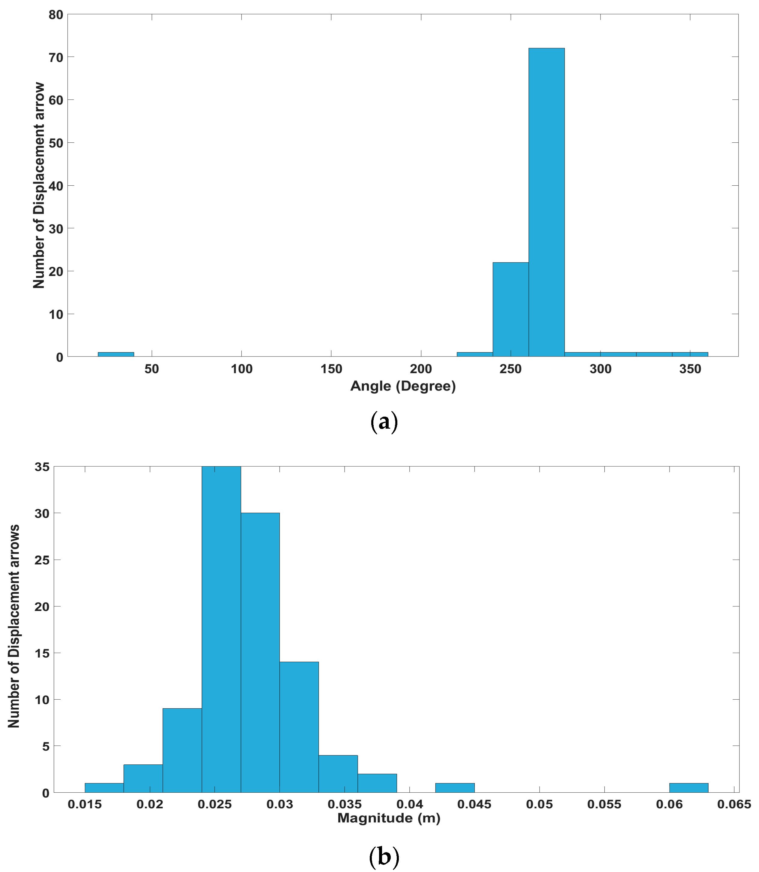
  • Reducing the errors caused by the matching process, especially in the border sections of the point cloud, by histogram analysis;
  • Maintaining proper distribution of vectors throughout the study areas;
  • Using various data to check the performance of the presented method more precisely. These data sets are different in size, type of deformation, density of point clouds, and direction of displacement;
  • Evaluation of the accuracy of the presented method using the available data.
This research paper is organized into seven sections. After the introduction, this research paper is organized into six sections. After the introduction, Section 2 provides a literature review of different methods for measuring landslides. Section 3 describes the data sets and methods used in this research. The research results are presented in Section 4 and discussed in Section 5. Section 6 summarizes the main conclusions.

2. Literature Review

This part of the research presents a comprehensive literature review of various methods for measuring landslides, including the Global Navigation Satellite System (GNSS), image-based monitoring, and TLS. Each method has its advantages and limitations, which will be discussed in detail. This review will provide insights into the applicability, accuracy, and reliability of these methods in landslide monitoring. In addition, this review will highlight recent advancements and research on combining different techniques to enhance the effectiveness of landslide monitoring.

2.1. Global Navigation Satellite System (GNSS)

GNSS sensors are one of the beneficial ways of monitoring landslides [18,19,20,21,22]. The GNSS technology has proved to be one of the most flexible and practical tools for monitoring purposes. These instruments enable precision at the centimeter level or even lower in static mode and lengthy observation times [23]. GNSS can offer precise and accurate data regarding the location and movement of landslides. By putting permanent GNSS receivers at strategic points on a landslide or in an area prone to landslides, it is possible to measure small-scale ground surface motions with high temporal resolution. GNSS may also be used to measure the velocity and acceleration of a landslide, which can provide important information about the landslide’s dynamics and possible risks and threats. The advances in GNSS technology have created new low-cost sensors that can provide continuous monitoring with medium to high precision, accuracy, and limited costs [23,24,25]. In this case, the precision of measuring is enough, but using these sensors for measuring the landslide provides low spatial resolution. Therefore, it is necessary to combine these sensors with other area-based methods to increase spatial resolution. It is possible to obtain a more comprehensive picture of a landslide and its development over time by combining GNSS data with the results of other remote sensing techniques, such as terrestrial laser scanning (TLS) and satellite images.
GNSS offers high precision in monitoring landslides, providing valuable data on location and movement. Its ability to measure velocities and accelerations is crucial for understanding landslide dynamics. However, its low spatial resolution necessitates integration with other methods for a comprehensive analysis.

2.2. Image-Based Monitoring

In addition to the accuracy needed to assess, with a given probability, the magnitude of the expected displacement and the number of other issues influence the choice of the best monitoring system to use. For instance, the size of the area to be controlled, the frequency of data gathering, the time it takes to provide the results, the stability of the reference system, and the impact of atmospheric conditions on measurement accuracy or operation [26].
Emerging Unmanned Aerial Vehicles (UAVs) are used for many purposes, including monitoring landslides. UAVs can provide high resolution compared to the first method. Furthermore, gathering data with them would be easier for large areas and regions that need to be monitored frequently during a short period. In most cases, UAVs use a camera to capture the images and make a 3D model from the area in each epoch [27,28,29,30,31]. With appropriate ground control, accuracies in the range of 3–10 cm in 3D can be expected, making UAV photogrammetry extremely appealing for monitoring applications [26,32]. Although most image-based methods in this field use airborne photogrammetry, some image-based research uses terrestrial systems [33,34,35]. Recent advancements in image-based methods have seen the rise of UAV-based Geographic Object-Based Image Analysis (GeoOBIA). This technique, utilizing high-resolution imagery from UAVs, allows for more detailed and frequent landslide assessments. A notable study in this area is the GeoBIA-based semi-automated landslide detection using UAV data [36], which demonstrates the potential of UAVs in enhancing spatial resolution and detection capabilities.
Satellite images are also used for monitoring landslides. Detecting and monitoring landslides can be accomplished in several different ways with the help of remote sensing methods, particularly satellite images. These methods have the potential to offer information regarding the location, extent, and movement of landslides, in addition to information regarding the dynamics and causes of landslides [14,37,38,39]. For instance, multispectral imagery, such as Landsat, can be applied to identify changes in vegetation cover and soil moisture, which can indicate the presence of a landslide, and radar imagery, such as that from the European Space Agency’s Sentinel-1 satellite, can be used to detect changes in the elevation of the ground surface caused by a landslide. There are also some disadvantages to this method when compared to point-based methods, and one of the primary concerns is the accuracy of the image-based method for landslide detection. As reported in [40], the accuracy ranged from 5 to 15 cm in several projects using different types of UAVs and cameras. In cases where landslides occur at a rate of several millimeters per year, the image-based method faces some serious challenges.
Image-based monitoring, bolstered by methods like UAV-based GeoOBIA, offers a unique perspective in landslide analysis, especially in identifying surface changes. While it faces challenges in accuracy, especially for slow-moving landslides, its integration with other methods can significantly improve overall monitoring effectiveness.

2.3. Terrestrial Laser Scanners

A fixed sensor known as a terrestrial laser scanner (TLS) automatically captures the range and angles in equally spaced scanning steps [41]. They use the laser’s flight time to compute distances to objects. Traditional measurement techniques do not have the advantages of three-dimensional laser scanning technology. It has high measurement accuracy and quick monitoring speed, can reflect the entire deformation trend of the landslide body, and can quickly produce high-precision, high-density three-dimensional point cloud data. It also does not need to touch the landslide body [42]. Consequently, numerous studies these days focus on using TLS for monitoring landslides [43,44,45,46,47,48]. However, this method also has some disadvantages, including a high volume of generated point clouds, especially for large areas, and the problem of accurately registering these point clouds. Based on this, there is some research about the reliability and accuracy of using TLS for monitoring [49,50]. In recent years, TLS and UAV photogrammetry have been used together to cover the disadvantages of using one of the methods alone [51,52,53,54,55].
The point clouds produced by laser scanners in two or more epochs are registered using different algorithms, such as ICP (Iterative closest point) [56] and M3C2 (multiscale model-to-model cloud comparison) [57], as well as their improved versions [58,59]. Feature matching is another method for matching the point clouds obtained from different epochs. This method is robust to noise in challenging conditions such as large-scale differences, and it can be used to register point clouds with a high degree of accuracy. This information can be used to monitor and evaluate the stability of places prone to landslides. Point cloud processing can provide vital information regarding potential landslide hazards, such as slope angles, surface roughness, and elevation changes, by examining the shape and structure of the terrain. This data can be used to construct detailed 3D models of the landscape and detect instability areas, which can aid in predicting and preventing landslides. In addition, point cloud analysis can be used to monitor changes in the terrain over time, which can aid in detecting early warning signals of landslides and tracking their advancement once they have occurred.
In this research, the feature-matching method proposed in [17] is used for the deformation analysis based on point clouds measured by terrestrial laser scanners. Additionally, a new component has been added to this algorithm to improve the accuracy and reliability of the results.
TLS stands out for its high accuracy and rapid data acquisition capabilities, producing detailed 3D point clouds. While handling large data volumes and registration accuracy can be challenging, the integration of TLS with UAV photogrammetry has been a significant leap forward, addressing individual limitations and enhancing landslide monitoring.

3. Materials and Methods

This research utilized three data sets collected in two epochs, and landslides were identified using the same method across all data sets. These data sets are different in several cases, including the size, material, georeferencing process, and displacement direction. Section 3.1 discusses the areas investigated in this study, while Section 3.2 outlines the method used to identify landslides.

3.1. Study Areas

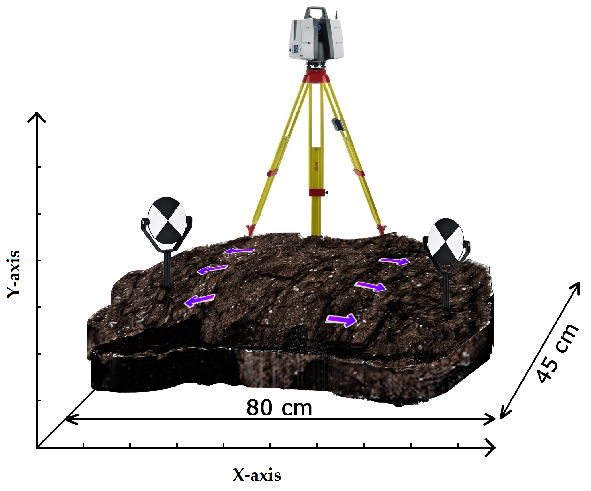
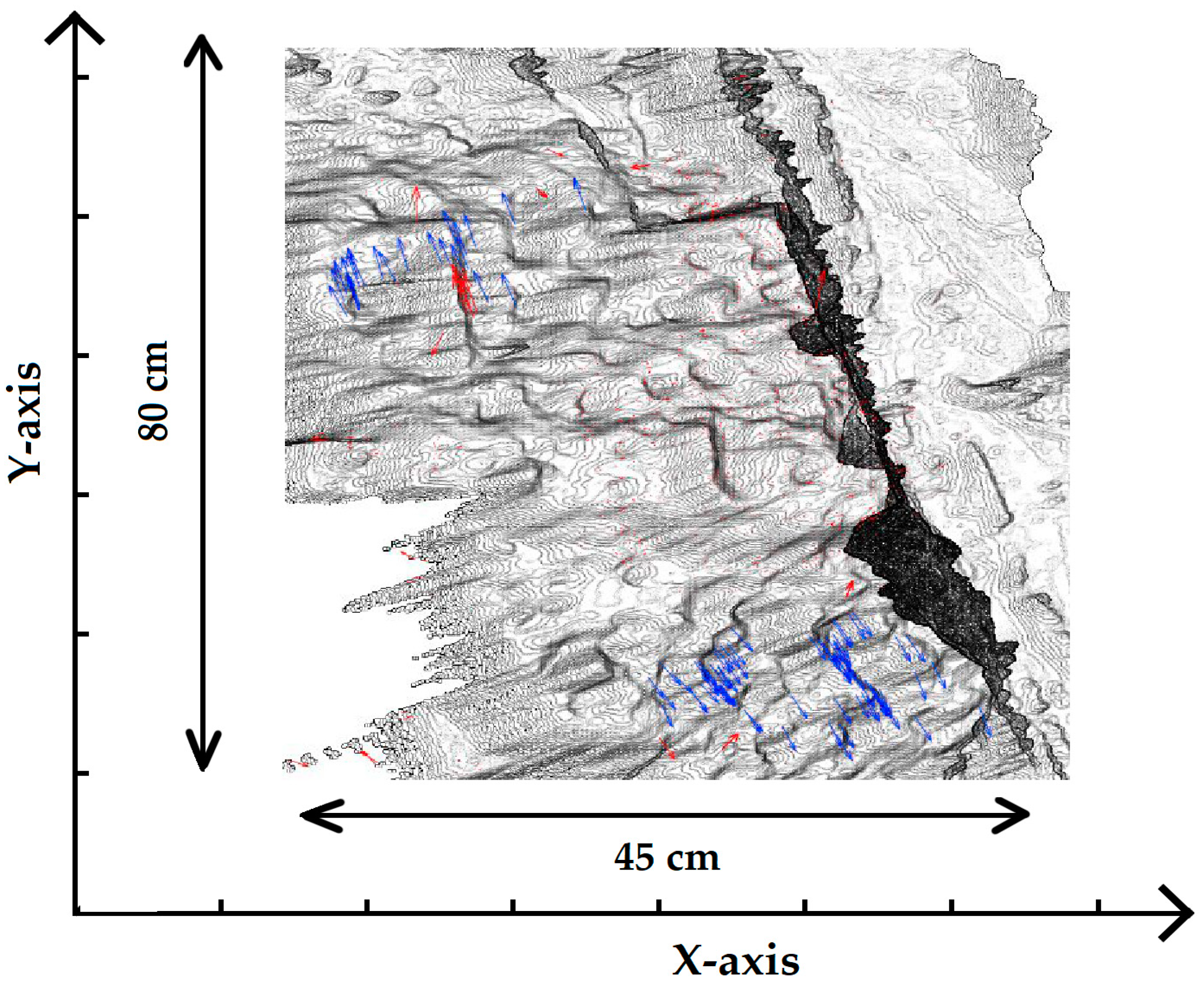
3.1.1. Simulated Laboratory Data Set

The first data set is a simulated laboratory data set. This data set was specifically selected for initial testing due to its controlled environment, which is ideal for an accurate assessment of the developed method. The purpose was to evaluate the precision of the scanner in detecting minute changes and to understand its capability to measure manual adjustments made on the surfaces. To generate this data set, we used a pack of soil to cover three designated separate surfaces (left, middle, and right) with an area of approximately 1 m in length and 0.5 m in width.
Next, a P50 laser scanner was placed on a tripod to measure a target on a compound slide at 5 m, with the goal of evaluating the scanner’s accuracy. The P50 was able to detect changes of approximately 0.1 mm on the target. Subsequently, the same targets were placed on the left and right surfaces, and the first epoch was captured using the highest resolution (0.8 mm per 10 m). For the second epoch, the P50’s position remained stable while movements were applied to the left and right surfaces, and the middle surface remained stationary. Epoch changes were made in two different directions, as depicted in Figure 1. The scanner station was positioned 5 m away from the area, enabling the P50 to produce dense and accurate point clouds.
It is essential to note that the changes in the data set were manually applied and measured using the targets placed on both surfaces. The scanner’s position was unchanged from the first epoch to the second, eliminating potential georeferencing errors that could impact the final accuracy achieved by this data set.

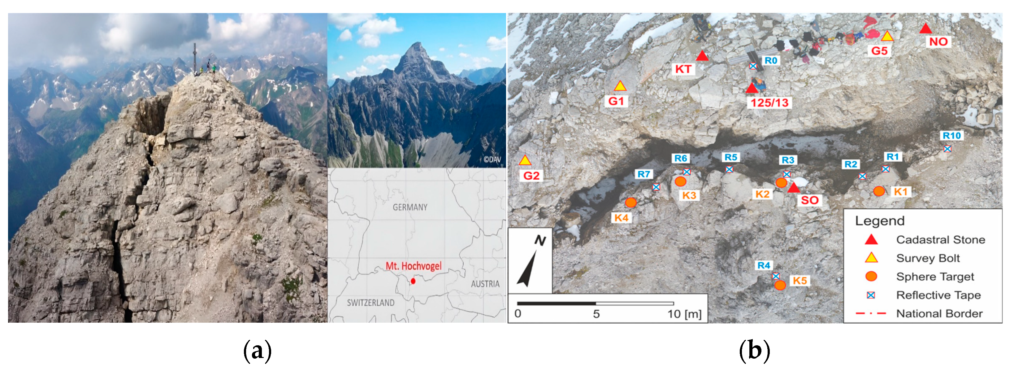
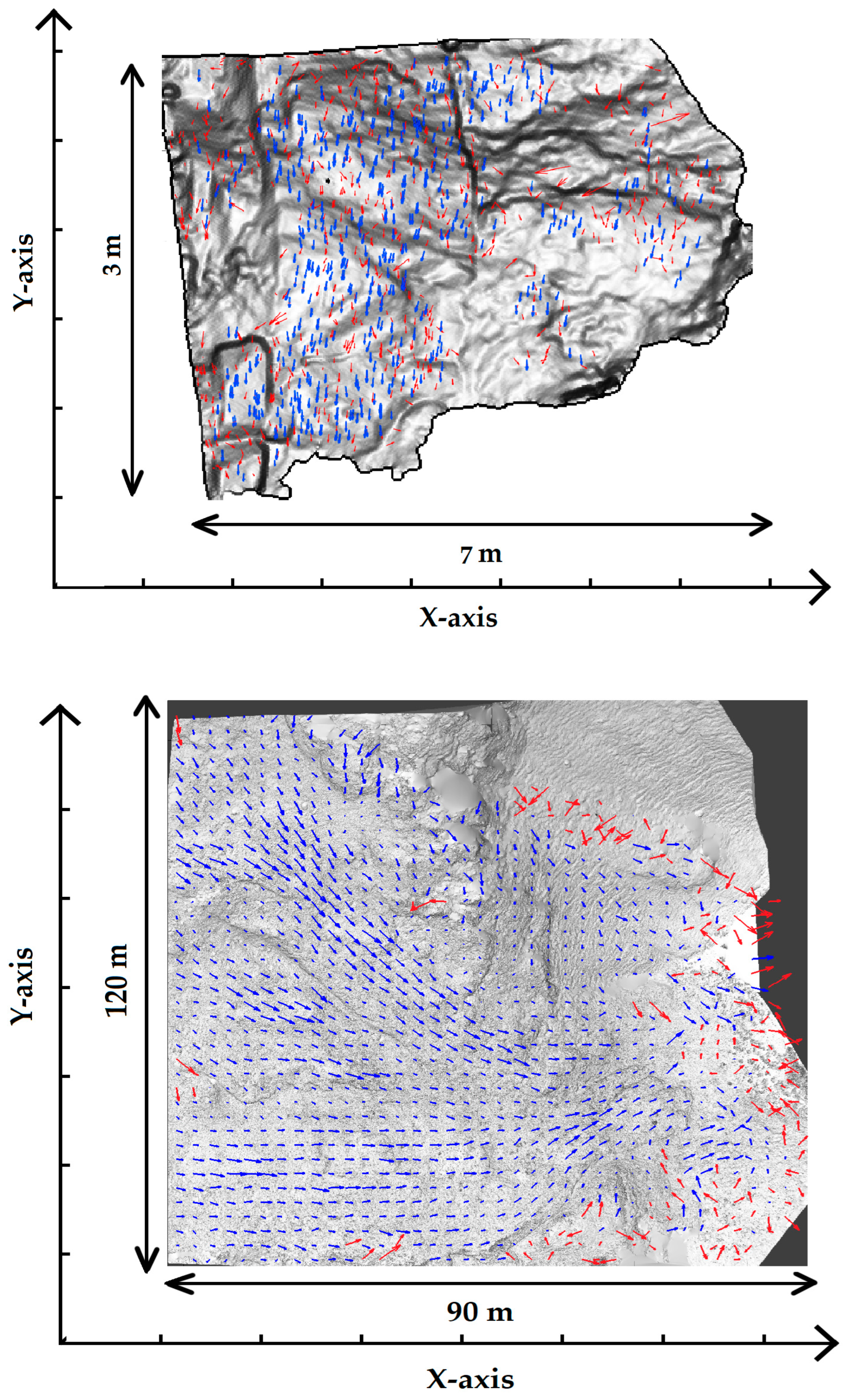
3.1.2. Hochvogel Data Set

The second data set is about the Hochvogel, a 2592-m-high mountain in the Allgäu Alps. The Hochvogel site was chosen because of its unique geological phenomena, offering a real-world setting for landslide monitoring. The data set from this area was particularly useful for studying the deterioration process and for testing the implementation of an early warning system, blending different measurement techniques. The mountain’s fame is based on a phenomenon observed on the Hochvogel for many decades. Part of the summit slowly breaks off at the top of the mountain on the German-Austrian border. It is the highest summit of the surrounding mountains and is therefore exposed to strong erosion [24]. This break-off is now visible at the summit in the form of a chasm about 30 m long and 3–5 m wide. The left part of the chasm consists of the breaking away rock. The crack between the two parts is much more resounding than visible from the outside because loose rocks fill the gap that narrows downwards (Figure 2). Upon closer examination, it becomes evident that the rock possesses a porous nature. Numerous small stones are not securely connected to the surrounding rock. However, several distinct rocks stand out, maintaining their shape despite weather conditions. These rocks are particularly interesting because their external structure remains consistent over extended periods, making certain surface parts recognizable in cross-epoch measurements. To better understand the ongoing deterioration process and implement an early warning system, several measurement systems were set up on the mountain, including a geodetic monitoring network [60]. This network combines tacheometric measurements with GNSS baseline observations, allowing for precise 3D vector determination in a deformation analysis based on a congruence model. The RTC360 laser scanner was used to collect this data set.
For the georeferencing process, a sufficient number of stable points were utilized to georeferenced data from different epochs. These points were visible in both epochs and were chosen on the stable part of this summit. The georeferencing accuracy was evaluated through a geodetic deformation analysis, revealing an approximate accuracy of around 2 mm [25]. This data set has already been used for point-wise rigorous deformation analysis. Therefore, one of the benefits of this data set is the ability to compare the results of the mentioned method with point-wise results.

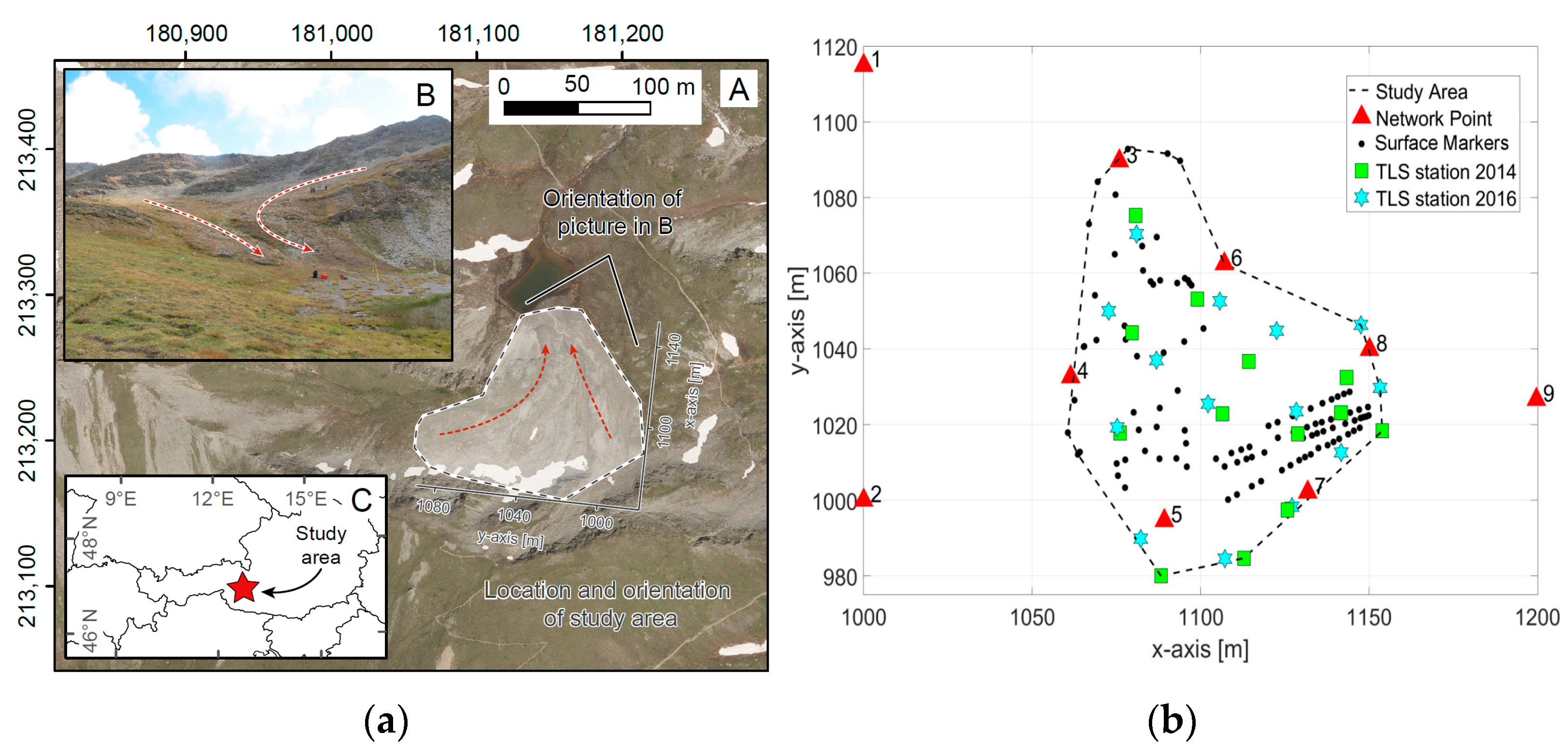
3.1.3. Hohe Tauern Data Set
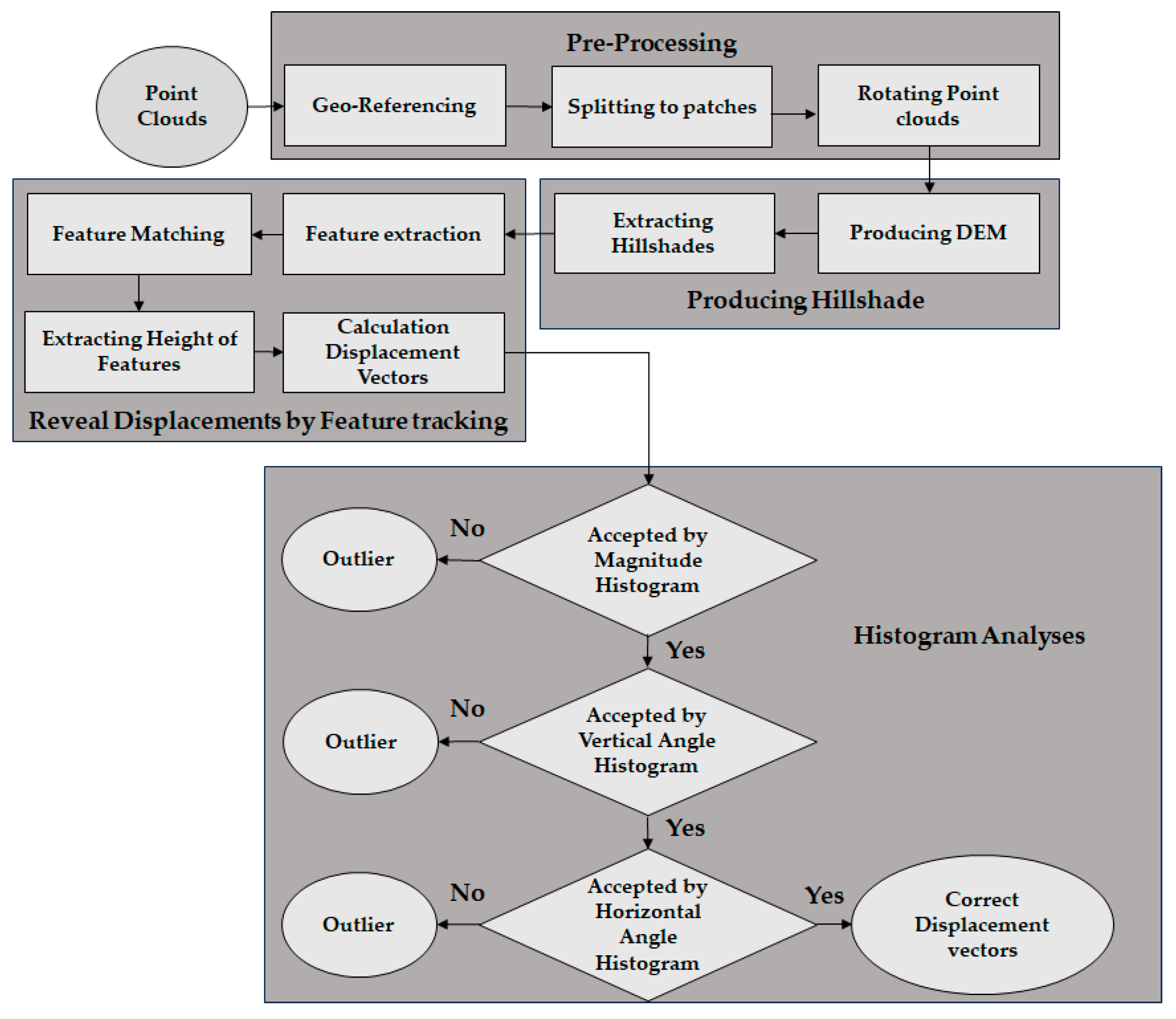
The third data set, located in the central Hohe Tauern range of the Austrian Alps, approximately 5 km south of the Großglockner (3798-m NHN, height above sea level), the highest peak in the Eastern Alps, has a distinct characteristic of deformation in different directions. Between 1985 and 2008, surface velocities were measured continuously using repeated GNSS surveys of more than 100 surface markers. The findings reveal significant variations in average velocities, ranging from 2 to 20 cm per year due to alpine solifluction. Additionally, peak velocities for individual markers reached up to 100 cm per year [16]. The study area, depicted in Figure 3, measures approximately 100 m on the x-axis and 100 m on the y-axis, with the deformation type being soil slope. The data sets were captured in 2014 and 2016, and to realize the local coordinate system, we permanently mounted nine points.
For georeferencing the point clouds, 9 fixed points were permanently marked with nails in the hard rock. Those fixed points were coordinated using relative GNSS-baseline measurements and total station measurements, all combined in a 3D geodetic network adjustment. The laser scans were transformed into this geodetic datum by centering scanner targets on those fixed points afterward. For potential transformation into an absolute coordinate system, we also occupied an official reference point of the Austrian geodetic reference frame. The position of each fixed point was chosen considering a homogeneous distribution over the complete study site and also good mutual visibility (total station and laser scanning) and sky visibility (GNSS). Incorporating these points into the network adjustment enhances the geometry and boosts the quality of the foundational geodetic network. However, the long-term stability of these points may be uncertain. They facilitate a more precise estimation of the relative positions of other stable points within each epoch [17].
This data set was also collected by the P50 laser scanner. The unique deformation patterns of this area make it an ideal location for studying slope movements and further analyses. Considering this area monitored by using a high spatial resolution method in 2021 [17], there are still some outliers present, which makes this data set interesting for this research.

3.2. Methodology

This section provides a rough overview of the sequence of actions in the algorithm, and the associated process chain is visualized in Figure 4. In general, the method is mainly automated regarding the processing of the point clouds, as it is necessary for an early warning system.
After measuring point clouds in two epochs, the pre-processing part starts. After georeferencing two point clouds, the first step involves reducing them to the expected area and removing extra parts. This is necessary to fragment the point clouds into smaller patches, which are then individually converted into digital elevation models (DEMs). The main reason for this is to prevent overlap during the production of a DEM. Considering that a specific projection direction is required to produce a digital elevation model, applying a single direction to the entire point cloud could result in overlap in certain parts. Consequently, some information may be lost due to this overlap (Figure 5).
To achieve this, the point clouds must be transformed such that the z-axis of the new coordinate system aligns with the direction from the laser scanner to the center of gravity of the individual patch for each epoch. If any other projection directions are considered, as shown in Figure 5 (top), there is a potential for overlap during the hillshade production process.
In the second section, hillshades are then produced for each of the two epochs DTMs. Point clouds are a valuable tool in producing high-resolution hillshades, providing an extremely detailed representation of the terrain surface. The process of creating hillshades from point clouds involves projecting the point cloud data into a two-dimensional plane and calculating the shading based on topographic features and the location of the sun. Hillshades provide a visual representation of the terrain that is much easier to understand than raw point cloud data, and the ability to adjust the direction and intensity of the simulated sunlight provides a powerful tool for visualizing and analyzing terrain features [61].
In the next section, features are extracted from the hillshades using the SIFT [62] and KAZE [63] feature extraction algorithms. Both algorithms are suitable for extracting features from the data, but KAZE generates more features compared to SIFT, so in this research, KAZE was utilized. Unlike earlier algorithms, KAZE uses non-linear scale spaces due to its use of non-linear diffusion filtering, which allows it to be more robust in terms of handling image noise and detecting features across various scales. It is important to note that having more features does not necessarily equate to higher quality. Extracting too many features could lead to high correlation among them and affect computational efficiency. The choice of a suitable feature extraction algorithm depends on several factors, including the size and texture of the study area. Notably, the texture of the area plays a significant role in the distribution and accuracy of the results.
Feature matching is then performed using SIFT to match the extracted features from the previous section. SIFT involves comparing the feature descriptors extracted from different images to find matches. These descriptors provide a unique fingerprint for different parts of an image, allowing the algorithm to identify the same features even when the viewpoint, scale, or lighting conditions change. Suitable height values are then extracted from the digital terrain models for the matched features in the first and second epochs, bringing the 2D features back into 3D space. This stage allows for determining the displacement values of characteristic object points.
It is important to note that a certain percentage of the matches are incorrect, meaning that a false match connects two features that do not represent the same point on the object’s surface. These incorrect matches can interfere with the qualitative and quantitative analysis of the results. Therefore, another section is required to complete the algorithm.
The last stage in this research involves the application of a histogram-oriented method for outlier removal after feature matching. This strategy proves vital in reducing the impact of unusual displacement vectors that could potentially distort data interpretation. A histogram is generated for each displacement vector and its neighboring vectors. This procedure is predicated on the hypothesis that displacement vectors within a confined area should not display substantial fluctuations in their magnitudes and directions. Subsequently, the absolute magnitude of each deformation vector is calculated, and a threshold is defined to separate significant outliers. Vectors with lengths less than or equal to this specific threshold value are included. The threshold is chosen based on any existing knowledge of the expected movement rates of the object under investigation. In the absence of such information, a higher threshold value is advocated to ensure the preservation of accurate matchings. For the Hochvogel, for example, it is known that between 2018 and 2021, the crumbling side of the summit is moving southwards at more than 2 cm per year. So, for three years, 6 to 8 cm can be expected. However, it can be more significant than what we expect. For the experiments within the framework of this work, the threshold value is generously set to 20 cm. This value was selected based on the expected movement rates of the monitored object. Considering the typical rate of displacement in landslide-prone areas, this threshold effectively separates significant movements from noise, ensuring accurate detection while minimizing false positives. For making this process automatic, it is possible to use the median of the displacement vectors as a trustable source because the number of significant outliers is not comparable with the total number of vectors.
The direction (both vertical and horizontal) and magnitude of the deformation vectors are investigated in relation to their neighboring vectors using three separate histograms. If a vector’s direction deviates significantly from those of its neighboring vectors, that vector is categorized as an outlier, justifying its removal. This strategy enhances the accuracy of the results by reducing the adverse effects of outliers. The same procedure is followed for the magnitudes of deformation vectors. As shown in Figure 6, the process involves generating histograms for each displacement vector and comparing it with its neighboring vectors. By doing so, any vector that deviates significantly from the overall pattern can be identified as an outlier.
In the first histogram (Figure 6a), it is evident that most displacement vectors fall within the range of 225° to 275° degrees. Therefore, if a particular vector’s direction is around 100 degrees, it would be considered an outlier due to its significant deviation from the prevailing trend. Similarly, in the second histogram (Figure 6b), most displacement vectors have magnitudes ranging from 2 to 3 cm. Consequently, if a specific vector exhibits a displacement magnitude of 6 cm, it would be identified as an outlier, once again, due to its substantial deviation from the typical range of magnitudes observed.
By utilizing this histogram analysis approach for each vector, the proposed method can effectively detect outliers in the displacement data, aiding in the refinement and improvement of the overall accuracy of the estimated displacement. While our methodology is robust for various terrains, it may have limitations in extremely rugged or densely vegetated areas, where laser scanning data might be less accurate. Additionally, the accuracy of our approach depends on the quality of the initial point cloud data. Any errors or inconsistencies in these data can propagate through the analysis, affecting the reliability of the results.

4. Results

In this section, we evaluated the accuracy of each step and its role in the final accuracy. Specifically, we examined producing hillshades and the matching processing and histogram analyses. A key aspect of our approach was the removal of mismatches, which is a common challenge in conventional monitoring methods. By incorporating histogram analyses, we sought to filter out these inaccuracies, thereby providing more trustworthy and precise results. The following results section demonstrates the efficacy of our method in achieving this goal.
Through a series of meticulous evaluations, we illustrate how our approach effectively minimizes errors and improves the overall accuracy of landslide monitoring. Each of these steps plays a crucial role in the final accuracy of the results, and it is important to assess their individual contributions. By understanding the accuracy of each step, we can identify areas that need improvement and optimize the entire process for the best possible results.

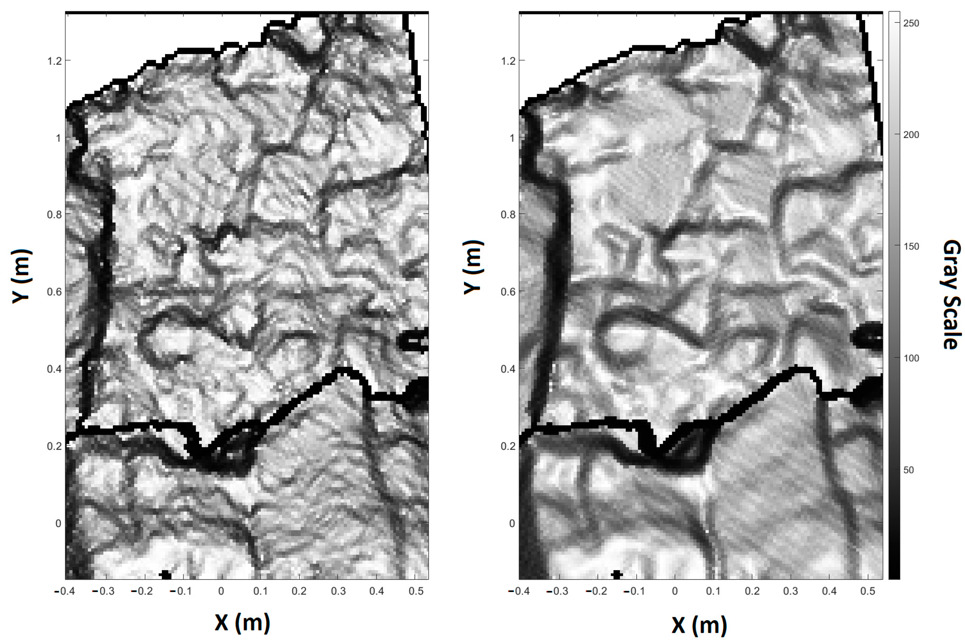
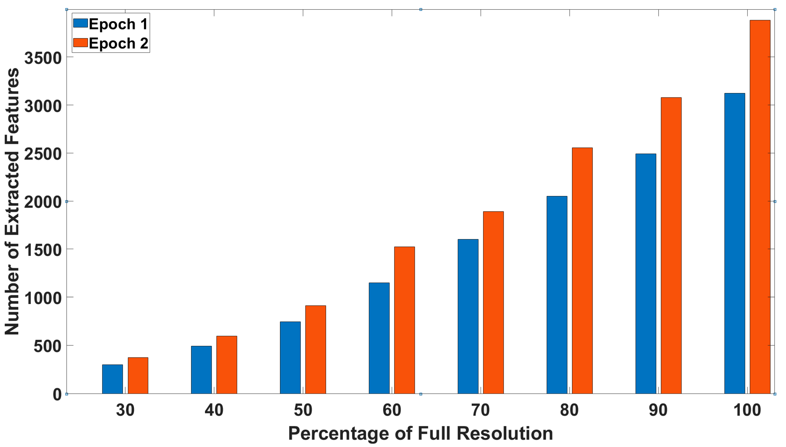
4.1. Producing Hillshades by Using Point Clouds

As mentioned in the previous section, hillshades are produced by using point clouds (Figure 7). The effect of hillshade resolution on the final accuracy was evaluated, and a decrease in accuracy was observed when the hillshade resolution was changed from 3 mm to 8 mm in the Hochvogel data set. This decrease is attributed to the loss of detail in the resulting hillshades (Figure 8). By reducing the resolution of the hillshades, as shown in Figure 9, we lose the detection and accurate location of many features. When the resolution is halved, the number of features detected using the same algorithm experiences a 75% reduction. This clearly illustrates the impact of hillshade resolution on spatial resolution.
Results show a reduction in the spatial resolution for displacement vectors and an increase in error when comparing the displacement of features and control points. As the point cloud becomes denser, the hillshades can display more and accurate features, resulting in improved accuracy in the final results. Therefore, it is crucial to ensure high-quality and dense point clouds to generate high-resolution hillshades that accurately represent the terrain features. In the Hochvogel data set, the point cloud from the second epoch is denser compared to the first epoch. This is why the number of detected features is 20% higher in this case.

4.2. Matching Process and Histogram Analyses

In this section, the matching algorithm was applied to the data sets. To begin, the features of hillshades in two epochs were extracted using the KAZE feature detection algorithm. Then, the matching between the features was performed using the SIFT algorithm. The results of the matching process revealed several incorrect matches, which, if left uncorrected, would negatively impact the accuracy of landslide detection and subsequent steps such as prediction and early warning systems. To mitigate these errors, it is crucial to implement a correction process to ensure the reliability of the results.
In this step, outliers were removed from the matching pairs through an analysis of their histograms. The results of the histogram analysis on the data set indicate that this step is critical for achieving accurate monitoring. The deformation monitoring would be improved by eliminating outliers, which represent the error in the matching process. According to Table 1, it is clear that the number of outliers in comparison to the whole displacement vectors is high, and it would definitely affect the final result if these vectors were not removed. In Figure 10, the positions of these outliers are also shown.

4.3. Accuracy Assessment

In order to assess the accuracy of the proposed method, the first data set generated in a laboratory was utilized to measure soil displacement. The displacement was measured in two distinct directions and then compared to the magnitude calculated using the proposed method. For measuring the applied displacement, two targets, which were automatically detected by the P50 laser scanner, were set on both sides of the data set (Figure 1). Displacement was then applied to the surfaces where the targets were set. The coordinates of the targets were captured both before and after applying this displacement. The shift that was applied to the data set is 17.1 mm to the right and a 13.9 mm shift to the left. Table 2 displays the various points that were detected and their corresponding movements, which were calculated using the proposed method.
The results of this evaluation are presented in Table 2. It shows the detected displacement for each point in the data set, along with the direction of the displacement. The calculated displacements are then compared to the applied displacements. From the table, it is evident that the proposed method shows differences between the detected and applied displacements ranging from 0.5 mm to 1.1 mm.
Several analyses were performed on the Hochvogel data set. Firstly, the accuracy of displacement arrows was compared with several points monitored by a total station. The average displacement detected in this data set was 2.6 cm with a standard deviation of 3.5 mm. By comparing the achieved accuracy with the accuracy obtained using the point-wise method in [24], it was found that the same level of accuracy was attained through histogram analysis at a higher resolution, which was one of the goals of this research.
The accuracy of the third data set (Hohe Tauern) was evaluated by comparing the displacement arrows extracted using the aforementioned method with those calculated using a total station at several checkpoints. The results indicate that the estimated vectors had a suitable level of accuracy (less than 10 mm). However, a large number of outliers were detected, necessitating further analysis using histogram analysis to refine the results.

5. Discussion

Based on the results of all the data sets, it is evident that utilizing the feature-based method for matching point clouds from different epochs enables the high spatial resolution of specific areas, which is useful for monitoring landslides through the prediction and early warning system. While it requires some necessary corrections, particularly in terms of feature matching, utilizing histogram analyses removes outliers and mismatches, thereby providing more trustworthy results, as shown in Figure 8. Additionally, this strategy helps maintain a proper distribution of vectors throughout the study areas, which is critical for effective monitoring and also leads to acceptable accuracy. To ensure the accuracy and quality of the results, we applied this method to three distinct data sets that varied in terms of land texture, area size, type of movement, and density of point clouds. The achieved accuracy in our data set ranged between 1 and 10 mm, which was influenced by the differences in the quality of the data sets. The laboratory data set resulted in the most accurate measurements as there were no errors in georeferencing, and a high-density point cloud was used due to the relatively small size of the data set. The accuracy of data sets is directly dependent on the degree of displacement, point cloud density in both epochs, the texture of the study area, type of movement, and the georeferencing process. For example, reducing the point cloud density by thirty percent and employing KAZE for feature extraction along with SIFT for feature matching resulted in a fifty percent decrease in the number of detected displacement vectors, underscoring the significance of this parameter.
Notably, some thresholds in the histogram analysis method should be defined depending on the area. For instance, if there were a large number of the detected features in the region, the number of neighbors that would be considered for each arrow could be higher than in the situation where the detected features are less and have a more considerable distance from each other. This threshold will affect the computation time and resources required for this process. Conversely, when eliminating apparent outliers prior to conducting histogram analyses, it is essential to set thresholds for displacement vector magnitudes based on the specific movements of the area under study. For instance, in an area with an average displacement of 5 cm per year, thresholds should be set at least three to four times greater than this average to prevent the inadvertent classification of genuine displacement vectors as outliers.
As described in Section 4, we applied the proposed process to three different data sets that varied significantly in terms of the time between epochs, distance, and scanning quality. We did this to develop a general algorithm that can be used on various data sets in the future for predicting the behavior of landslides. We also used a laboratory data set to precisely monitor the accuracy of this method, which was successful. By using this data set, we were able to measure the displacement that was applied to the data set before using the method. Consequently, we regard it as an appropriate means to assess the method’s accuracy.
It is crucial to consider that the accuracy of the georeferencing and matching process can significantly impact the overall accuracy of the project. For example, In the second data set, the inclusion of the georeferencing process impacted the final accuracy, introducing errors approximately 2 mm in magnitude due to complexities encountered during this stage. Moreover, the point cloud density produced by the laser scanner can influence the accuracy and level of detail in the hillshade, which serves as the foundation for feature extraction in this method. SIFT is specifically designed to match key points between images with subpixel accuracy, and the pixel size directly depends on the point cloud density. Hence, the point cloud density and the laser scanner’s accuracy are critical factors in achieving reasonable final accuracy.
While the method has proven effective across three distinct data sets, it faces challenges in certain conditions and terrains. Dense vegetation, for instance, can impede the identification of key surface points. Moreover, the method’s reliance on feature extraction means that the proximity of the laser scanner to the targeted area significantly influences the level of detail captured. Consequently, greater distances between the scanner and the area pose additional challenges to the method’s effectiveness. The efficacy of this method has been validated for data sets collected within a 300 m range; however, its applicability to greater distances remains untested.

6. Conclusions and Outlook

In this research, we developed a method for monitoring landslides with high resolution and removing outliers, which has a significant impact on accuracy and future improvements. By using this method, we were able to achieve trustworthy and accurate results in monitoring landslides with terrestrial laser scanners. This accuracy could be between 1 to several mm depending on the quality of the data set and conditions. The findings of this study have the potential to greatly improve our understanding of landslides and the methods used to monitor them. The results demonstrate the benefits of using high spatial resolution techniques to monitor landslides. The georeferencing process, hillshade creation, matching process, and histogram analyses conducted as part of the study provide a comprehensive examination of the data sets used. The results of these analyses give a clear picture of the behavior of the landslides and provide insights into the key factors that contribute to their development and evolution. The information gathered from this study can be used to develop more effective landslide monitoring strategies and to better understand the mechanisms driving landslide behavior.
One of the weaknesses of this method that could be improved in the future is its complete reliance on feature extraction, which makes it difficult to extract features in areas with smooth transitions. To overcome this limitation, larger areas could be utilized with the aid of aerial and satellite images to extract additional features from larger areas by employing various image processing techniques, we can enhance the utility of UAV and satellite imagery for large-scale movement detection. It is important to consider, however, that these methods may not capture details as precisely as laser scanners. Moreover, this method is a practical system for monitoring landslides that have already occurred. Implementing real-time landslide prediction systems presents several key challenges. These include the need for accurate and comprehensive data collection, the deployment and maintenance of sensor networks in often rugged terrain, and the requirement for sophisticated data processing capabilities. By utilizing the results of this method and incorporating additional elements, such as real-time data collection and analysis, this system could be adapted for predicting landslides in the future, which would be the ultimate goal. Predictive capabilities would enable more effective planning and mitigation efforts and potentially save lives and property. This research is part of a project aimed at monitoring landslides in an area near the railway, known for its history of landslides. The goal of this project is to enhance an early warning system that assists trains passing through this area by providing information on whether the rail track is at risk of being blocked.

Author Contributions

K.H. and L.R. (Leonhard Reindl); methodology, K.H. and L.R. (Leonhard Reindl); software, K.H.; validation, K.H., C.H. and W.W.; formal analysis, K.H. and L.R. (Leonhard Reindl); investigation, K.H. and L.R. (Leonhard Reindl); resources, C.H., L.R. (Lukas Raffle) and K.H.; data curation, C.H., L.R. (Lukas Raffle) and K.H.; writing—original draft preparation, K.H.; writing—review and editing, K.H. and C.H.; visualization, K.H.; supervision, C.H.; project administration, C.H. and K.H.; funding acquisition, C.H. All authors have read and agreed to the published version of the manuscript.

Funding

The German Federal Ministry of Education and Research (BMBF) is funding the AImon5.0 project within the funding measure “Digital GreenTech—Environmental Engineering meets Digitalisation” as part of the “Research for Sustainability’ (FONA) Strategy”. This project is also funded by the Bavarian State Ministry of the Environment and Consumer Protection within the “AlpSenseRely” project.

Data Availability Statement

Restrictions apply to the availability of these data. Data was obtained by using the resources which funded by The German Federal Ministry of Education and Research (BMBF) and are available from the authors with the permission of The German Federal Ministry of Education and Research (BMBF).

Conflicts of Interest

The authors declare no conflict of interest.

References

  1. Long, J.; Li, C.; Liu, Y.; Feng, P.; Zuo, Q. A Multi-Feature Fusion Transfer Learning Method for Displacement Prediction of Rainfall Reservoir-Induced Landslide with Step-like Deformation Characteristics. Eng. Geol. 2022, 297, 106494. [Google Scholar] [CrossRef]
  2. Mizutori, M.; Guha-Sapir, D. Economic Losses, Poverty and Disasters 1998–2017; United Nations Office for Disaster Risk Reduction: Geneva, Switzerland, 2017; Volume 4, pp. 9–15. [Google Scholar]
  3. Yin, Y.; Liu, X.; Zhao, C.; Tomás, R.; Zhang, Q.; Lu, Z.; Li, B. Multi-Dimensional and Long-Term Time Series Monitoring and Early Warning of Landslide Hazard with Improved Cross-Platform SAR Offset Tracking Method. Sci. China Technol. Sci. 2022, 65, 1891–1912. [Google Scholar] [CrossRef]
  4. Zhang, Y.; Tang, J.; Cheng, Y.; Huang, L.; Guo, F.; Yin, X.; Li, N. Prediction of Landslide Displacement with Dynamic Features Using Intelligent Approaches. Int. J. Min. Sci. Technol. 2022, 32, 539–549. [Google Scholar] [CrossRef]
  5. Jiang, S. Study of Landslide Geological Hazard Prediction Method Based on Probability Migration. Nat. Hazards 2021, 108, 1753–1762. [Google Scholar] [CrossRef]
  6. Ma, J.; Xia, D.; Guo, H.; Wang, Y.; Niu, X.; Liu, Z.; Jiang, S. Metaheuristic-Based Support Vector Regression for Landslide Displacement Prediction: A Comparative Study. Landslides 2022, 19, 2489–2511. [Google Scholar] [CrossRef]
  7. Leinauer, J.; Weber, S.; Cicoira, A.; Beutel, J.; Krautblatter, M. Towards Prospective Failure Time Forecasting of Slope Failures. In Proceedings of the EGU General Assembly Conference Abstracts 2022, Vienna, Austria, 23–27 May 2022; p. EGU22-7673. [Google Scholar] [CrossRef]
  8. Ma, P.; Cui, Y.; Wang, W.; Lin, H.; Zhang, Y. Coupling InSAR and Numerical Modeling for Characterizing Landslide Movements under Complex Loads in Urbanized Hillslopes. Landslides 2021, 18, 1611–1623. [Google Scholar] [CrossRef]
  9. Tayyebi, S.M.; Pastor, M.; Stickle, M.M.; Yagüe, Á.; Manzanal, D.; Molinos, M.; Navas, P. SPH Numerical Modelling of Landslide Movements as Coupled Two-Phase Flows with a New Solution for the Interaction Term. Eur. J. Mech.-BFluids 2022, 96, 1–14. [Google Scholar] [CrossRef]
  10. Heidarzadeh, M.; Ishibe, T.; Sandanbata, O.; Muhari, A.; Wijanarto, A.B. Numerical Modeling of the Subaerial Landslide Source of the 22 December 2018 Anak Krakatoa Volcanic Tsunami, Indonesia. Ocean Eng. 2020, 195, 106733. [Google Scholar] [CrossRef]
  11. Xu, Y.; George, D.L.; Kim, J.; Lu, Z.; Riley, M.; Griffin, T.; de la Fuente, J. Landslide Monitoring and Runout Hazard Assessment by Integrating Multi-Source Remote Sensing and Numerical Models: An Application to the Gold Basin Landslide Complex, Northern Washington. Landslides 2021, 18, 1131–1141. [Google Scholar] [CrossRef]
  12. Jutz, B.K. Bergstürze in den Alpen mit Beispielen aus dem Ötztal; University Vienna: Vienna, Austria, 2012. [Google Scholar]
  13. Hungr, O.; Leroueil, S.; Picarelli, L. The Varnes Classification of Landslide Types, an Update. Landslides 2014, 11, 167–194. [Google Scholar] [CrossRef]
  14. Edrich, A.-K.; Yildiz, A.; Roscher, R.; Kowalski, J. A Modular and Scalable Workflow for Data-Driven Modelling of Shallow Landslide Susceptibility. In Proceedings of the EGU General Assembly Conference Abstracts 2022, Vienna, Austria, 23–27 May 2022; p. EGU22-4900. [Google Scholar] [CrossRef]
  15. Donati, D.; Rabus, B.; Engelbrecht, J.; Stead, D.; Clague, J.; Francioni, M. A Robust SAR Speckle Tracking Workflow for Measuring and Interpreting the 3D Surface Displacement of Landslides. Remote Sens. 2021, 13, 3048. [Google Scholar] [CrossRef]
  16. Strupler, M.; Anselmetti, F.S.; Hilbe, M.; Kremer, K.; Wiemer, S. A Workflow for the Rapid Assessment of the Landslide-Tsunami Hazard in Peri-Alpine Lakes. Geol. Soc. Lond. Spec. Publ. 2020, 500, 81–95. [Google Scholar] [CrossRef]
  17. Holst, C.; Janßen, J.; Schmitz, B.; Blome, M.; Dercks, M.; Schoch-Baumann, A.; Blöthe, J.; Schrott, L.; Kuhlmann, H.; Medic, T. Increasing Spatio-Temporal Resolution for Monitoring Alpine Solifluction Using Terrestrial Laser Scanners and 3D Vector Fields. Remote Sens. 2021, 13, 1192. [Google Scholar] [CrossRef]
  18. Carlà, T.; Tofani, V.; Lombardi, L.; Raspini, F.; Bianchini, S.; Bertolo, D.; Thuegaz, P.; Casagli, N. Combination of GNSS, Satellite InSAR, and GBInSAR Remote Sensing Monitoring to Improve the Understanding of a Large Landslide in High Alpine Environment. Geomorphology 2019, 335, 62–75. [Google Scholar] [CrossRef]
  19. Paziewski, J.; Sieradzki, R.; Baryla, R. Multi-GNSS High-Rate RTK, PPP and Novel Direct Phase Observation Processing Method: Application to Precise Dynamic Displacement Detection. Meas. Sci. Technol. 2018, 29, 035002. [Google Scholar] [CrossRef]
  20. Melgar, D.; Melbourne, T.I.; Crowell, B.W.; Geng, J.; Szeliga, W.; Scrivner, C.; Santillan, M.; Goldberg, D.E. Real-Time High-Rate GNSS Displacements: Performance Demonstration during the 2019 Ridgecrest, California, Earthquakes. Seismol. Res. Lett. 2020, 91, 1943–1951. [Google Scholar] [CrossRef]
  21. Capilla, R.M.; Berné, J.L.; Martín, A.; Rodrigo, R. Simulation Case Study of Deformations and Landslides Using Real-Time GNSS Precise Point Positioning Technique. Geomat. Nat. Hazards Risk 2016, 7, 1856–1873. [Google Scholar] [CrossRef]
  22. Gümüş, K.; Selbesoğlu, M.O. Evaluation of NRTK GNSS Positioning Methods for Displacement Detection by a Newly Designed Displacement Monitoring System. Measurement 2019, 142, 131–137. [Google Scholar] [CrossRef]
  23. Poluzzi, L.; Tavasci, L.; Corsini, F.; Barbarella, M.; Gandolfi, S. Low-Cost GNSS Sensors for Monitoring Applications. Appl. Geomat. 2020, 12, 35–44. [Google Scholar] [CrossRef]
  24. Notti, D.; Cina, A.; Manzino, A.; Colombo, A.; Bendea, I.H.; Mollo, P.; Giordan, D. Low-Cost GNSS Solution for Continuous Monitoring of Slope Instabilities Applied to Madonna Del Sasso Sanctuary (NW Italy). Sensors 2020, 20, 289. [Google Scholar] [CrossRef]
  25. Raffl, L.; Holst, C. Including Virtual Target Points from Laser Scanning into the Point-Wise Rigorous Deformation Analysis at Geo-Monitoring Applications. In Proceedings of the 5th Joint International Symposium on Deformation Monitoring-JISDM 2022, València, Spain, 20–22 June 2022; Editorial de la Universitat Politècnica de València: Valencia, Spain, 2022. [Google Scholar] [CrossRef]
  26. Dall’Asta, E.; Forlani, G.; Roncella, R.; Santise, M.; Diotri, F.; Morra di Cella, U. Unmanned Aerial Systems and DSM Matching for Rock Glacier Monitoring. ISPRS J. Photogramm. Remote Sens. 2017, 127, 102–114. [Google Scholar] [CrossRef]
  27. Eichel, J.; Draebing, D.; Kattenborn, T.; Senn, J.A.; Klingbeil, L.; Wieland, M.; Heinz, E. Unmanned Aerial Vehicle-based Mapping of Turf-banked Solifluction Lobe Movement and Its Relation to Material, Geomorphometric, Thermal and Vegetation Properties. Permafr. Periglac. Process. 2020, 31, 97–109. [Google Scholar] [CrossRef]
  28. Cenni, N.; Fiaschi, S.; Fabris, M. Integrated Use of Archival Aerial Photogrammetry, GNSS, and InSAR Data for the Monitoring of the Patigno Landslide (Northern Apennines, Italy). Landslides 2021, 18, 2247–2263. [Google Scholar] [CrossRef]
  29. Vanderhorst, H.R. Method of Applying Unmanned Aerial Vehicle (UAV) for Landslides Identification in the Dominican Republic. Preprint; In Review. 2022. Available online: https://www.researchsquare.com/article/rs-1653879/v1 (accessed on 17 July 2023).
  30. Đorđević, D.R.; Đurić, U.; Bakrač, S.T.; Drobnjak, S.M.; Radojčić, S. Using Historical Aerial Photography in Landslide Monitoring: Umka Case Study, Serbia. Land 2022, 11, 2282. [Google Scholar] [CrossRef]
  31. Lian, X.; Li, Z.; Yuan, H.; Liu, J.; Zhang, Y.; Liu, X.; Wu, Y. Rapid Identification of Landslide, Collapse and Crack Based on Low-Altitude Remote Sensing Image of UAV. J. Mt. Sci. 2020, 17, 2915–2928. [Google Scholar] [CrossRef]
  32. Peppa, M.V.; Mills, J.P.; Moore, P.; Miller, P.E.; Chambers, J.E. Accuracy assessment of a uav-based landslide monitoring system. In Proceedings of the International Archives of the Photogrammetry, Remote Sensing and Spatial Information Sciences, Volume XLI-B5, 2016 XXIII ISPRS Congress, Prague, Czech Republic, 12–19 July 2016; pp. 895–902. [Google Scholar] [CrossRef]
  33. Roncella, R.; Forlani, G.; Fornari, M.; Diotri, F. Landslide Monitoring by Fixed-Base Terrestrial Stereo-Photogrammetry. ISPRS Ann. Photogramm. Remote Sens. Spat. Inf. Sci. 2014, II–5, 297–304. [Google Scholar] [CrossRef]
  34. Cardenal, J.; Mata, E.; Perez-Garcia, J.L.; Delgado, J.; Hernandez, M.A.; Gonzalez, A.; Diaz-de-Teren, J.R. Close Range Digital Photogrammetry Techniques Applied to Landslide Monitoring. Int. Arch. Photogramm. Remote Sens. Spat. Inf. Sci. 2008, 37, 235–240. [Google Scholar]
  35. Lucks, L.; Hirt, P.-R.; Hoegner, L.; Stilla, U. Photogrammetric Monitoring of Gravitational Mass Movements in Alpine Regions by Markerless 3D Motion Capture. Int. Arch. Photogramm. Remote Sens. Spat. Inf. Sci. 2022, XLIII-B2-2022, 1063–1069. [Google Scholar] [CrossRef]
  36. Kundal, S.; Chowdhury, A.; Bhardwaj, A.; Garg, P.K.; Mishra, V. GeoBIA-Based Semi-Automated Landslide Detection Using UAS Data: A Case Study of Uttarakhand Himalayas. In Proceedings of the SPIE Conferences, Boston, MA, USA, 18–19 April 2023; Volume 12327, pp. 321–329. [Google Scholar] [CrossRef]
  37. Ullo, S.L.; Langenkamp, M.S.; Oikarinen, T.P.; Del Rosso, M.P.; Sebastianelli, A.; Piccirillo, F.; Sica, S. Landslide Geohazard Assessment with Convolutional Neural Networks Using Sentinel-2 Imagery Data. In Proceedings of the IGARSS 2019–2019 IEEE International Geoscience and Remote Sensing Symposium; IEEE: Yokohama, Japan, 2019; pp. 9646–9649. [Google Scholar] [CrossRef]
  38. König, T.; Kux, H.J.H.; Mendes, R.M. Shalstab Mathematical Model and WorldView-2 Satellite Images to Identification of Landslide-Susceptible Areas. Nat. Hazards 2019, 97, 1127–1149. [Google Scholar] [CrossRef]
  39. Wasowski, J.; Bovenga, F. Remote Sensing of Landslide Motion with Emphasis on Satellite Multi-Temporal Interferometry Applications. In Landslide Hazards, Risks, and Disasters; Elsevier: Amsterdam, The Netherlands, 2022; pp. 365–438. [Google Scholar] [CrossRef]
  40. Hussain, Y.; Schlögel, R.; Innocenti, A.; Hamza, O.; Iannucci, R.; Martino, S.; Havenith, H.-B. Review on the Geophysical and UAV-Based Methods Applied to Landslides. Remote Sens. 2022, 14, 4564. [Google Scholar] [CrossRef]
  41. Kermarrec, G.; Yang, Z.; Czerwonka-Schröder, D. Classification of Terrestrial Laser Scanner Point Clouds: A Comparison of Methods for Landslide Monitoring from Mathematical Surface Approximation. Remote Sens. 2022, 14, 5099. [Google Scholar] [CrossRef]
  42. Jiang, S.; Deng, X.; Chen, M. 3-D Laser Scanning Landslide Deformation Monitoring and Data Processing Based on Computer Cluster. J. Phys. Conf. Ser. 2019, 1345, 062039. [Google Scholar] [CrossRef]
  43. Pesántez Cabrera, P.C. Land Movement Detection from Terrestrial Laser Scanner (LiDAR) Analysis. In Laser Radar Technology and Applications XXVI; Turner, M.D., Kamerman, G.W., Eds.; SPIE: Online, USA, 2021; p. 17. [Google Scholar] [CrossRef]
  44. Ozdogan, M.V. Landslide Detection and Characterization Using Terrestrial 3D Laser Scanning (LiDAR). Acta Geodyn. Geomater. 2019, 16, 379–392. [Google Scholar] [CrossRef]
  45. Zhao, L.; Ma, X.; Xiang, Z.; Zhang, S.; Hu, C.; Zhou, Y.; Chen, G. Landslide Deformation Extraction from Terrestrial Laser Scanning Data with Weighted Least Squares Regularization Iteration Solution. Remote Sens. 2022, 14, 2897. [Google Scholar] [CrossRef]
  46. Guo, Y.; Li, X.; Ju, S.; Lyu, Q.; Liu, T. Utilization of 3D Laser Scanning for Stability Evaluation and Deformation Monitoring of Landslides. J. Environ. Public Health 2022. [Google Scholar] [CrossRef] [PubMed]
  47. Pesántez, P.C. Landslide Study Using Terrestrial Laser Scanner (Lidar) Analysis. Int. Arch. Photogramm. Remote Sens. Spat. Inf. Sci. 2020, XLIII-B3-2020, 1251–1256. [Google Scholar] [CrossRef]
  48. Jaboyedoff, M.; Derron, M.-H. Landslide Analysis Using Laser Scanners. In Developments in Earth Surface Processes; Elsevier: Amsterdam, The Netherlands, 2020; Volume 23, pp. 207–230. [Google Scholar] [CrossRef]
  49. Abbas, M.A.; Fuad, N.A.; Idris, K.M.; Opaluwa, Y.D.; Hashim, N.M.; Majid, Z.; Sulaiman, S.A. Reliability of Terrestrial Laser Scanner Measurement in Slope Monitoring. IOP Conf. Ser. Earth Environ. Sci. 2019, 385, 012042. [Google Scholar] [CrossRef]
  50. Zeybek, M.; Şanlıoğlu, İ. Accurate Determination of the Taşkent (Konya, Turkey) Landslide Using a Long-Range Terrestrial Laser Scanner. Bull. Eng. Geol. Environ. 2015, 74, 61–76. [Google Scholar] [CrossRef]
  51. Boyd, J.; Chambers, J.; Wilkinson, P.; Peppa, M.; Watlet, A.; Kirkham, M.; Jones, L.; Swift, R.; Ulhemann, S.; Holmes, J.; et al. Coupling Terrestrial Laser Scanning and UAV Photogrammetry with Geoelectrical Data for Better Time-Lapse Hydrological Characterisation of an Active Landslide. In Proceedings of the EGU General Assembly 2022, Vienna, Austria, 23–27 May 2022. [Google Scholar] [CrossRef]
  52. Ji, H.; Luo, X. 3D Scene Reconstruction of Landslide Topography Based on Data Fusion between Laser Point Cloud and UAV Image. Environ. Earth Sci. 2019, 78, 534. [Google Scholar] [CrossRef]
  53. Zheng, X.; Yang, X.; Ma, H.; Ren, G.; Yu, Z.; Yang, F.; Zhang, H.; Gao, W. Integrative Landslide Emergency Monitoring Scheme Based on GB-INSAR Interferometry, Terrestrial Laser Scanning and UAV Photography. J. Phys. Conf. Ser. 2019, 1213, 052069. [Google Scholar] [CrossRef]
  54. Jiang, N.; Li, H.; Hu, Y.; Zhang, J.; Dai, W.; Li, C.; Zhou, J.-W. A Monitoring Method Integrating Terrestrial Laser Scanning and Unmanned Aerial Vehicles for Different Landslide Deformation Patterns. IEEE J. Sel. Top. Appl. Earth Obs. Remote Sens. 2021, 14, 10242–10255. [Google Scholar] [CrossRef]
  55. Jiang, N.; Li, H.-B.; Li, C.-J.; Xiao, H.-X.; Zhou, J.-W. A Fusion Method Using Terrestrial Laser Scanning and Unmanned Aerial Vehicle Photogrammetry for Landslide Deformation Monitoring Under Complex Terrain Conditions. IEEE Trans. Geosci. Remote Sens. 2022, 60, 4707214. [Google Scholar] [CrossRef]
  56. Besl, P.J.; McKay, N.D. Method for Registration of 3-D Shapes. In Proceedings of the SPIE Conferences, Boston, MA, USA, 14–15 November 1991; pp. 586–606. [Google Scholar] [CrossRef]
  57. Lague, D.; Brodu, N.; Leroux, J. Accurate 3D Comparison of Complex Topography with Terrestrial Laser Scanner: Application to the Rangitikei Canyon (N-Z). ISPRS J. Photogramm. Remote Sens. 2013, 82, 10–26. [Google Scholar] [CrossRef]
  58. Winiwarter, L.; Anders, K.; Höfle, B. M3C2-EP: Pushing the Limits of 3D Topographic Point Cloud Change Detection by Error Propagation. ISPRS J. Photogramm. Remote Sens. 2021, 178, 240–258. [Google Scholar] [CrossRef]
  59. Yang, Y.; Schwieger, V. Supervoxel-Based Targetless Registration and Identification of Stable Areas for Deformed Point Clouds. J. Appl. Geod. 2022, 17, 161–170. [Google Scholar] [CrossRef]
  60. Thomas Wunderlich, L.R. Challenges and Hybrid Approaches in Alpine Rockslide Prevention—An Alarming Case Study; INGEO&SIG: Tamil Nadu, India, 2020; p. 129. [Google Scholar]
  61. Horn, B.K.P. Hill Shading and the Reflectance Map. Proc. IEEE 1981, 69, 14–47. [Google Scholar] [CrossRef]
  62. Lowe, D.G. Distinctive image features from scale-invariant keypoints. Int. J. Comput. Vis. 2004, 60, 91–110. [Google Scholar] [CrossRef]
  63. Alcantarilla, P.F.; Bartoli, A.; Davison, A.J. KAZE features. In Proceedings of the Computer Vision–ECCV 2012: 12th European Conference on Computer Vision, Florence, Italy, 7–13 October 2012; Proceedings, Part VI 12. Springer: Berlin/Heidelberg, Germany, 2012; pp. 214–227. [Google Scholar]
Figure 1. The laboratory data set (displacement applied in two different directions, which is shown by purple arrows).
Remotesensing 16 00138 g001
Figure 2. (a) Summit of the Hochvogel, far view, and (b) different point’s positions at this summit [25].
Remotesensing 16 00138 g002
Figure 3. (a) Location and orientation of study area (Hohe Tauern) and (b) arrangement of points and stations on the local coordinate system [17].
Remotesensing 16 00138 g003
Figure 4. A rough overview of the algorithm. It included 4 main sections: Pre-processing, Producing hillshade, Reveal displacements by feature tracking, and Histogram analyses.
Remotesensing 16 00138 g004
Figure 5. Overlaps can occur when choosing a single projection direction (top). These overlaps can be avoided by creating patches (bottom).
Remotesensing 16 00138 g005
Figure 6. (a) Horizontal angle and (b) magnitude histograms for one of the displacement arrows and its neighbors in the Hohe Tauern data set.
Remotesensing 16 00138 g006
Figure 7. Part of Hochvogel’s point cloud and the hillshade that is produced. This figure shows how hillshade is extracted from a point cloud.
Remotesensing 16 00138 g007
Figure 8. Hillshade from the same area (Hochvogel) with 100% (right) and 70% (left) resolution.
Remotesensing 16 00138 g008
Figure 9. The number of extracted features is based on hillshade resolution. Blue and orange colors show the first and second epochs, which were captured from the same area (Hochvogel).
Remotesensing 16 00138 g009
Figure 10. The result of applying histogram analyses on data sets is shown. All arrows are magnified with a scale of 20 to enhance visibility, with the red arrows being removed as outliers by the proposed algorithm.
Remotesensing 16 00138 g010aRemotesensing 16 00138 g010b
Table 1. Number of total displacement arrows and percentage of outliers.
Data SetDisplacement VectorsOutliersPercentage of Outliers
Laboratory1383626.1%
Hochvogel106816915.8%
Hohe Tauern122032226.4%
Table 2. Comparison of displacement in sample points and the area.
Point NumberDetected Displacement (mm)DirectionThe Difference with the Applied Displacement (mm)The Ratio of Error to Magnitude
116.2Right0.95.2%
216.3Right0.84.6%
316.9Right1.16.4%
416.6Right0.52.9%
513.4Left0.64.3%
613.0Left1.07.1%
713.3Left0.64.3%
Disclaimer/Publisher’s Note: The statements, opinions and data contained in all publications are solely those of the individual author(s) and contributor(s) and not of MDPI and/or the editor(s). MDPI and/or the editor(s) disclaim responsibility for any injury to people or property resulting from any ideas, methods, instructions or products referred to in the content.

