Developing a Method to Automatically Extract Road Boundary and Linear Road Markings from a Mobile Mapping System Point Cloud Using Oriented Bounding Box Collision-Detection Techniques

Abstract

Advancements in data-acquisition technology have led to the increasing demand for high-precision road data for autonomous driving. Specifically, road boundaries and linear road markings, like edge and lane markings, provide fundamental guidance for various applications. Unfortunately, their extraction usually requires labor-intensive manual work, and the automatic extraction, which can be applied universally for diverse curved road types, presents a challenge. Given this context, this study proposes a method to automatically extract road boundaries and linear road markings by applying an oriented bounding box (OBB) collision-detection algorithm. The OBBs are generated from a reference line using the point cloud data’s position and intensity values. By applying the OBB collision-detection algorithm, road boundaries and linear road markings can be extracted efficiently and accurately in straight and curved roads by adjusting search length and width to detect OBB collision. This study assesses horizontal position accuracy using automatically extracted and manually digitized data to verify this method. The resulting RMSE for extracted road boundaries is +4.8 cm and +5.3 cm for linear road markings, indicating that high-accuracy road boundary and road marking extraction was possible. Therefore, our results demonstrate that the automatic extraction adjusting OBB detection parameters and integrating the OBB collision-detection algorithm enables efficient and precise extraction of road boundaries and linear road markings in various curving types of roads. Finally, this enhances its practicality and simplifies the implementation of the extraction process.

1. Introduction

With the development of data-acquisition technology, the utilization of high-precision data in fields such as digital twins and automatic driving has expanded significantly. Among the various surveying techniques for acquiring high-precision data, such as aerial and drone photogrammetry and ground surveys, light detection and ranging (LiDAR) has been widely used. LiDAR has higher transmittance than general cameras and can acquire precise data without being affected by weather or time. LiDAR has been used in fields such as dimensional modeling and map production. Sensors mounted on a terrestrial Mobile Mapping System (MMS) include positioning sensors, such as global navigation satellite systems (GNSS), inertial navigation systems (INS), distance measurement instruments (DM), and vision sensors, such as digital cameras. Therefore, the point cloud data collected with the MMS can store geometric attributes such as position (x, y, z) and optical properties such as intensity or color (RGB) using these sensors [1].

Because the point cloud data collected with a Mobile Mapping System (MMS) contains the location information of lane-level road objects, such as road markings, traffic signs, or roadside furniture, it is widely applied to construct high-precision road maps for autonomous driving. Specifically, road boundaries and linear road markings, such as edge and lane markings, provide important guidance and play fundamental roles in various applications; however, the extraction process generally entails manual and time-consuming work. Concerning its essential role and decisive functionality, a method for automatically extracting road boundaries and linear road markings must be developed to increase work efficiency.

Given this context, this study aims to develop a method to improve and increase the work efficiency of manual-work-dependent extraction of continuous road boundaries and linear road markings, including lane and edge markings, by applying an automatic extraction method. In this study, the reference lines of road boundaries and linear road markings create oriented bounding boxes (OBBs), rectangles with directionality, using the position and intensity values. Based on OBBs, this study aims to apply a collision algorithm to automatically extract road boundaries and linear road markings from point cloud data.

This paper is structured as follows. Section 2 presents an overview of relevant previous studies within the scope of this research. Section 3 introduces a detailed description of the proposed method for creating OBBs of road boundaries and linear road markings and automatically extracting them by applying the OBB collision-detection algorithm. Section 4 compares the extracted results with manually digitized data and verifies the proposed method. Finally, Section 5 discusses some of the limitations of this study and directions for improvement, highlighting the contributions of this study.

2. Literature Review

Edge detection and linear feature extraction from the 3D point cloud data were conducted [2,3,4,5,6,7,8,9,10,11,12,13,14,15,16,17,18,19,20,21,22,23,24,25,26]. This section presents an analysis of previous research and an examination of their limitations and suggestions, leading to the derivation of an improved method for automatically extracting linear data from point cloud data.

Many mathematical algorithms for estimating model parameters or clustering analyses have been applied to extract linearity from point clouds [4,12,14,18,20,22,25,27,28,29,30,31]. Most importantly, the least-squares method is a technique for estimating the regression coefficient, which is one of the ways to minimize errors and is mainly used to derive patterns from data (Figure 1). It can be used when the value cannot be accurately measured intuitively and is also the most commonly used technique in linear regression. However, calculating all data has the disadvantage of deriving incorrect values that include abnormal values (error values and noise) or increasing the amount of calculation according to the amount of data.

Random sample consensus (RANSAC) is a representative method among various analyses. RANSAC is a methodology proposed by Foley et al. (1981) initially for use in computer vision [26]. RANSAC is mainly used for predicting model parameters from original data containing many noisy errors and extracting linear data from these data. It randomly selects values from the original data, repeats the process of predicting the optimal parameters, and finds a fitting model. RANSAC classifies the data into inliers and outliers. An inlier is a value included in the data distribution, and an outlier is an error value that deviates considerably from the data distribution (Figure 1). Unlike the least-squares method, which calculates values outside the threshold, RANSAC enables more precise linear data extraction and random sampling. Although this method could quickly estimate the model, the results were random (Figure 1). Because of the nature of point cloud data, many data types are noisy, and various researchers have applied the RANSAC algorithm to derive optimal results from noisy data. Specifically, to extract linear features, most automatic feature extraction studies have utilized the RANSAC algorithm.

The point cloud data collected in a road environment contain linear features representing road boundaries and linear road markings on the pavement. Numerous studies have been conducted to derive boundaries by extracting the edges of a plane from point cloud data. Clustering points can generate planes with similar angles; their edges are extracted by connecting the lines where the planes meet. For example, Gross et al. (2006) [33] constructed a plane using the covariance matrix of the height and normal line in the laser point cloud data and compared the vector’s dot product to extract the plane’s boundary to create a line. However, there are limitations to highly accurate boundary line extraction as a method for generating the roof and exterior of a building. Yang et al. (2010) [28] studied a planar sensing method by integrating RANSAC and the minimum description length (MDL). They calculated the parameters of the plane equation by randomly selecting three points. Then, they created a plane by detecting points belonging to the calculated plane according to a given threshold. They extracted planes from each block using MDL to determine the number of planes in each block and merged neighboring planes to create the entire plane. Although the plane detection probability increased in a complex 3D point cloud, and the road boundary of a straight section could be extracted, the accuracy was low for turning sections of the road.

Tran et al. (2013) [19] studied a method for automatically extracting sharp feature lines using the surface normal vectors of point cloud data. Using the normal vector and distance, the outlines of the complex structures are extracted by selecting the surrounding point cloud using information such as the point cloud. This method can extract a linear line with a low error rate, even from a point cloud with noise. Bazazian et al. (2015) [27] studied a method for extracting boundaries from unorganized point cloud data. Generally, geometric features, such as normal vectors and curvatures, must be extracted for boundary recognition. A clustering method was used to determine the edges because sufficient information about the geometry cannot be obtained using normal data alone. First, they attempted area extraction with clustering using the k-NN algorithm and detected edge features by analyzing the eigenvalues of the covariance matrix defined with this method. This method requires less time than the edge extraction method when applying triangulation. Similarly, Ni et al. (2016) [29] studied a method for extracting lines by detecting boundaries and analyzing the geometrical characteristics of 3D point cloud data. This method, called the analysis of geometric properties of neighborhoods (AGPN), uses RANSAC and a method for detecting edges by measuring angular intervals by analyzing the geometric properties of point groups. Precise boundary lines can be extracted through a boundary search. However, excessive segmentation occurs with strict input values or long linear data.

Furthermore, Miyazaki et al. (2017) [22] studied a line-based region growth method for extracting a plane region with precise boundaries from point cloud data with an anisotropic distribution. The RANSAC algorithm was applied by generating line segments to measure the exact edges of a planar structure. By connecting the points with a polyline and calculating the normal vector for each line segment, the road area can be appropriately extracted from the point cloud data using the difference between the turbulence vector of the line segment belonging to the surface forming the road and the largest boundary stone. However, extraction errors occur at locations with noisy data, such as bushes. Tian et al. (2022) [20] studied to extract three-dimensional line segments from unstructured building-point data. Data pre-processing was performed through sampling, filtering, and projection, and a projection method was used to divide the vertical and horizontal planes of the point group. Subsequently, the boundary point is extracted by projecting all points belonging to each side onto the plane using the alpha shape algorithm, and the line is extracted quickly and accurately by extracting and merging the three-dimensional line segment structure from the boundary point. Because this method is performed in a two-dimensional space through projection, it can operate efficiently compared with Region Growing and RANSAC. High-accuracy results are derived even in complex structures. Moreover, the line features can be extracted from the RGB information of the point cloud data by applying RASNAC [25].

With the development of deep learning, studies have been conducted to extract features using deep learning neural networks for semantic segmentation [2,20,31,34,35,36,37,38]. Kukolj et al. (2021) [12] proposed a method to detect road edges by combining deep learning and spatial statistics. Instead of filtering point cloud data using attribute values, they obtained point cloud data on the road surface using deep learning semantic segmentation. They then converted the segmented point cloud data into 3D voxel grids with spatial statistics and clustered the filtered voxels based on geometric characteristics to extract road edges. Xu et al. (2022) [39] proposed a neural network for extracting multi-scale features from an overhead catenary system (OCS) point cloud by applying semantic segmentation. They manually annotated semantic information on the collected OCS point cloud dataset. They trained the deep learning model to classify each point into nine classes of catenary wire and oblique cantilever, according to attributes, including location $(x,y,z)$, color (RGB), and intensity values. However, in addition to PointNet++ [38], owing to the sparse distribution of the point cloud, the linear features of OCSs, such as the catenary wire, must be improved by supplementing the catenary characteristics. Similarly, after extracting the support positioning devices (SPD) in the catenary system using a new point spacing-based spatial clustering of applications with noise (PSBSCAN) algorithm, Zhang et al. (2023) [2] retrieved the spatial relationship between the extracted features and railway devices using a spatial index with semantic information. The indexing rule is based on a multiple-level voxel segmentation algorithm. In particular, by classifying the voxels into three groups—linear, nonlinear, and empty—the linear state of the feature could be efficiently detected.

Intensity values have been widely used in many studies to extract road markings because of the highly reflective material on paints. Chen et al. (2009) [18] generated 2D images using the intensity of point cloud data, filtered the lanes, and used RANSAC to identify lanes in road areas. This method performed well for deteriorated roads where the lanes were visually unclear. Zeybek (2021) [16] proposed a semi-automated extraction method for road markings from a 3D point cloud using a mobile laser scanning system, such as linear road markings and road arrows. The point cloud data were coarsely classified as either ground or non-ground points using a Cloth Simulation Filtering algorithm. Zhang et al. (2019) [30] employed RANSAC to fit a plane to ground point cloud data, and the optimally fitted plane could be regarded as the road surface. Subsequently, by comparing the distance between the surface with all points and the road, the points representing other features, such as curves or moving cars, can be determined and removed.

After filtering the point cloud data, the intensity threshold that separated the asphalt road surface and linear road markings was calculated. The areas of the linear road markings were determined using density-based spatial clustering (DBSCAN). Then, the method applied the alpha ($\alpha$) shapes algorithm to each clustered point to extract boundary points, which could drive road markings in 3D space. Similarly, after leaving the point cloud data on the road surface using Cloth Simulation Filtering, Chang et al. (2023) [14] classified the point cloud data into asphalt road surfaces and road markings by filtering them based on the Otsu threshold and clusters using Euclidean. After creating oriented bounding boxes (OBB) from each cluster, the method classifies them according to geometric characteristics, such as length and width, and extracts the markings by type.

Yang et al. (2020) [6] applied a median filter to the intensity values to suppress the noise caused by decreased road marking points as the scanning distance increased. After smoothing the intensity values of the markings, rapid intensity gradients were used to detect the edges of the markings. However, because the range of intensity values for road marking extraction varies locally depending on the weather and road conditions, a strategy to determine the appropriate intensity threshold is required to extract markings. In this context, Cheng et al. (2020) [11] are linked with an intensity normalization method for lane extraction that can be utilized independently of the environmental conditions. However, this method lacks a simplified range of values according to the hypothesis that the intensity values would be homogeneous for the same surface. However, extraction based on the intensity value with clustering depends on the road pavement conditions, such as markings’ fading and points’ density. Lin et al. (2021) [4] extracted lane markings using a linear density-based clustering method to overcome this limitation. After diving the ground for several trips, the optimal angle of the stripe with the highest density of lane marking points is identified. This method can extract the maximum linear density of pavement from lane markings on low-density roadsides. However, this method can only be applied to straight lines.

In addition to utilizing intensity values, Gao et al. (2017) [13] integrated multiple-attribute information, such as RGB color and position $(x,y,z)$, to extract pavement markings. First, road features were acquired based on point cloud elevation differences. They then converted the RGB color image into a grayscale image and calculated the grayscale difference to detect the boundaries of heterogeneous objects. After dividing it into two classes based on a threshold from the Otsu algorithm, road markings were extracted using intensity differences. This study showed that fusing multiple attributes can increase the accuracy and completeness of road marking extraction.

However, some studies have converted intensity values into images. Kang et al. (2020) [3] generated RGB images using the intensity and height of the point cloud data and filtered them to extract road markings on the map. Furthermore, with the advancement of deep learning, deep learning-based approaches have been used to extract and classify road markings integrated with intensity images [5,7,9,11]. However, deep-learning-based approaches require much training data robust to environmental conditions, such as weather.

Moreover, some studies have extracted road marking features in a vector format by transforming 3D points into 2D images [31,40]. Prochazka et al. (2019) [31] used the dynamic bound box principle to derive the lowest points in point cloud data and extract lines. Subsequently, the study utilized the RANSAC algorithm to subdivide them based on the Euclidean distance. For lane marking area extraction, they used an alpha-shape algorithm to create a contour line and a spanning tree to extract lanes. This method automatically extracted lanes; however, the method was unsuitable for use in complex road intersections and exhibited limitations in extracting mainly parallel lines. Lin et al. (2015) [24] designed a method to accurately extract plane intersection lines from large-scale unstructured point cloud data. They converted point cloud data into shaded images and extracted 2D line areas using a line segment detector (LSD) algorithm. Then, they back-projected the data to a 3D line area containing one line segment in each area, and then they extracted linear data according to the line segment half-planes (LSHP) structure. Although this method can extract lines from complex point cloud data, the area visualized in the point cloud data for the analysis is sensitive to the rendering resolution. Lu et al. (2019) [23] developed a method for rapidly extracting linear 3D parts from point cloud data. Unlike the method of extracting point clouds at the boundary and linearly connecting them, point clouds are segmented and projected onto a plane to form a 2D image from which 2D lines are detected. The detected 2D line was projected onto a 3D plane to detect the 3D lines. Linearity was quickly extracted with this method; however, in the case of curved surfaces, distortion occurred in the projection; therefore, these surfaces could not be adequately extracted.

Several studies have utilized road design regulations to extract lane markings. For example, Ye et al. (2022) [10] defined the positions of lane marking points by calculating their distances from road edges. Road markings can be extracted according to their width in the road design standard. Lane markings on a curved road can be extracted by splitting the curved road into short blocks. Similarly, Ma et al. (2019) [21] developed a semi-automatic method for extracting a horizontal curved line from mobile laser scanning (MLS). Using a curvature analysis, the study implemented a spline curve fitting to road segments with angles between the start and end points of the curve to extract the curved line efficiently. However, this method is only available for curved roads and cannot extract them well if there is a noise value at the road boundary.

Various studies have been conducted to extract linear features from point cloud data, and RANSAC, which extracts lines by removing noise, has been widely used. According to previous studies, when using the method of calculating point clouds at all positions within the range to be extracted as a line, the amount of calculation is excessive, even if it is extracted as a line after removing noise, which creates challenges in extracting a straight line at an exact position. For example, in the case of a straight line, a line can be obtained by evenly moving the position after checking the direction without calculating the points for all values or fine noisy data. In addition, criteria must be defined to extract points to accurately create a line from the points that comprise a road surface, and a method must be developed to minimize errors in areas with large amounts of noise and missing data.

Therefore, this study develops a method to automatically extract road boundaries and linear road markings, namely edge and lane markings, by applying an oriented bound box (OBB) collision-detection algorithm. The oriented bounding box (OBB) is a rectangular box that surrounds a cluster of points with a directionality. These were generated using normal vectors and intensity values based on a reference line. Using these OBBs, the proposed method detects collisions and automatically extracts road boundaries and linear road markings.

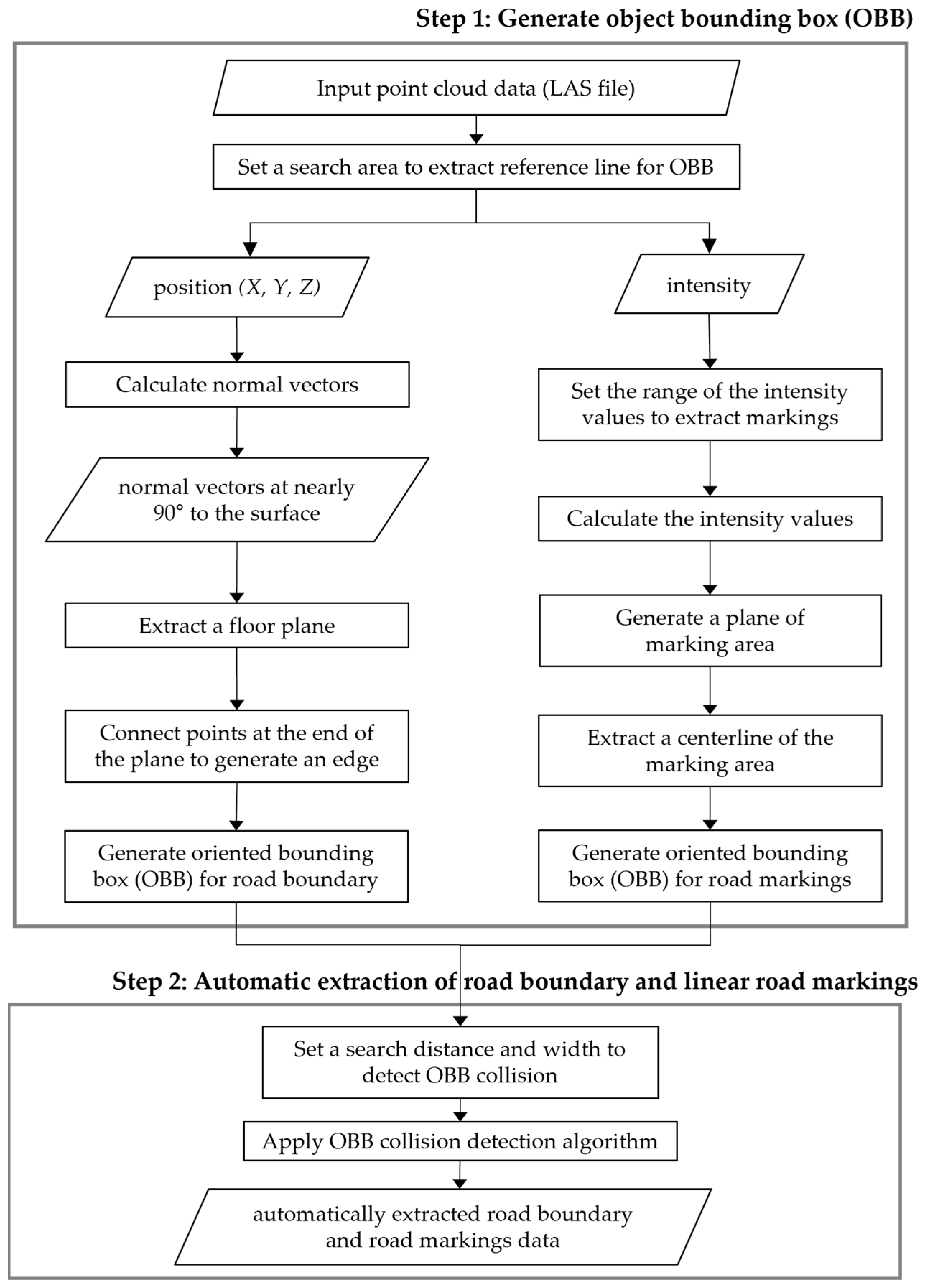
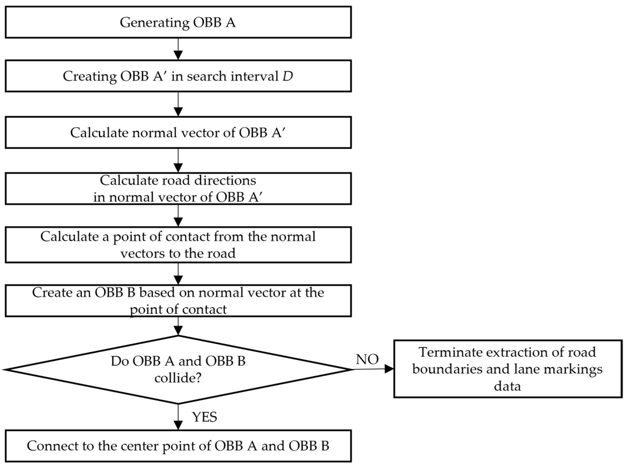
3. Method of Automatic Road Boundary and Linear Road Marking Extraction

This section describes a method for automatically extracting road boundaries and linear markings from point cloud data. Figure 2 illustrates a flowchart of this method. The proposed methodology includes creating an oriented bounding box (OBB) for the markings and automatically extracting them by applying the OBB collision-detection algorithm (Figure 2). First, to generate the OBBs, the search area for extracting a reference line must be set. The reference lines of each road boundary and linear road marking were obtained using the position and intensity values. Based on the created OBBs, step 2 sets a search distance and width to detect collisions between OBBs. Then, we applied a collision-detection algorithm to automatically extract road boundaries and linear road markings from point cloud data.

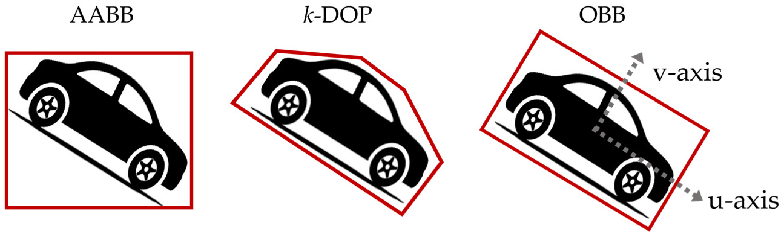
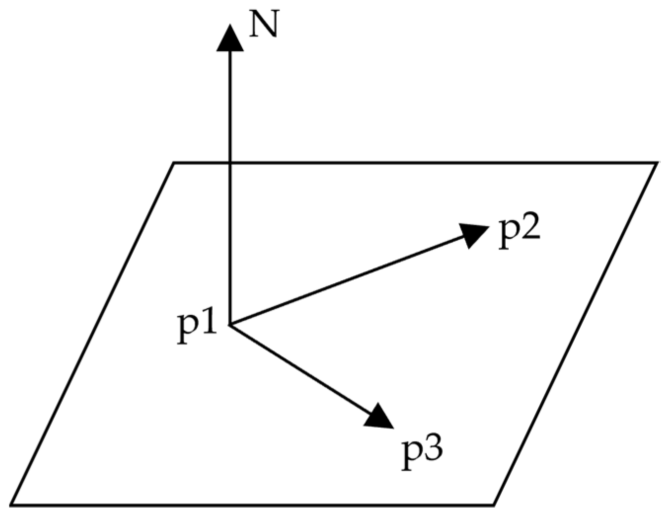
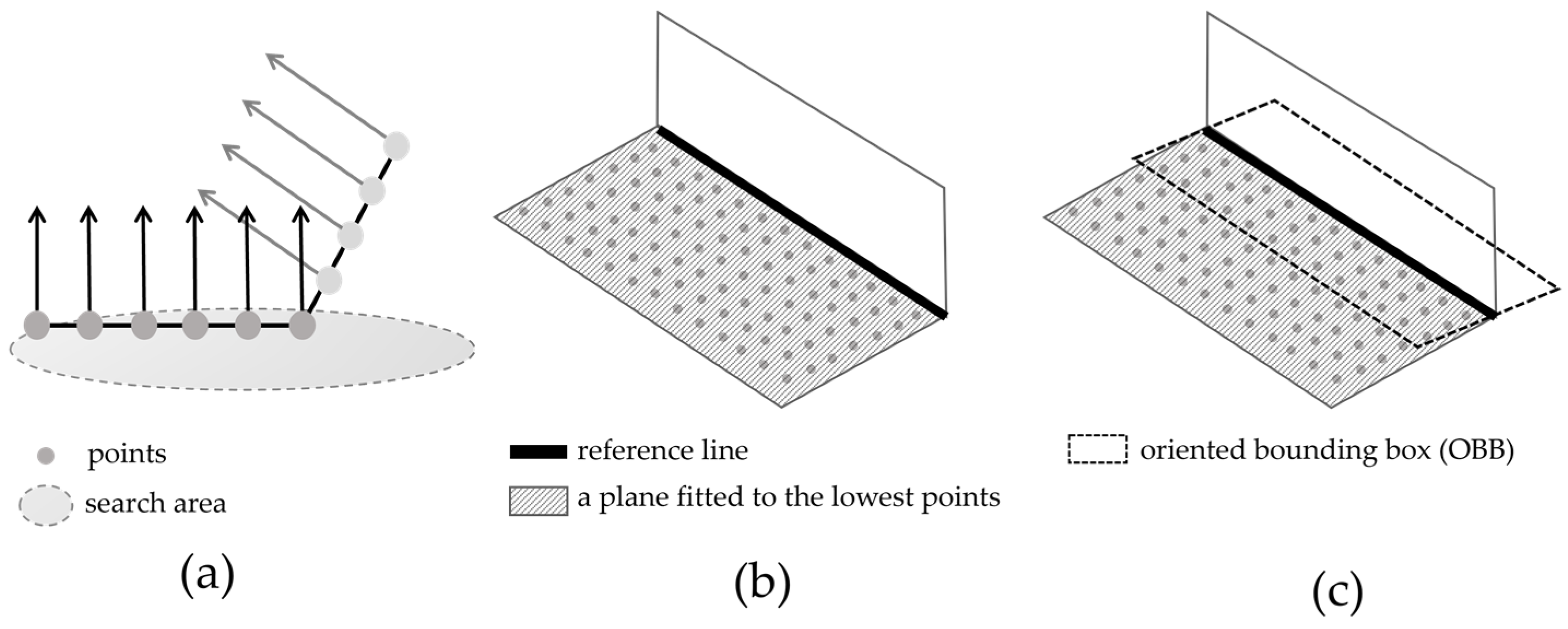
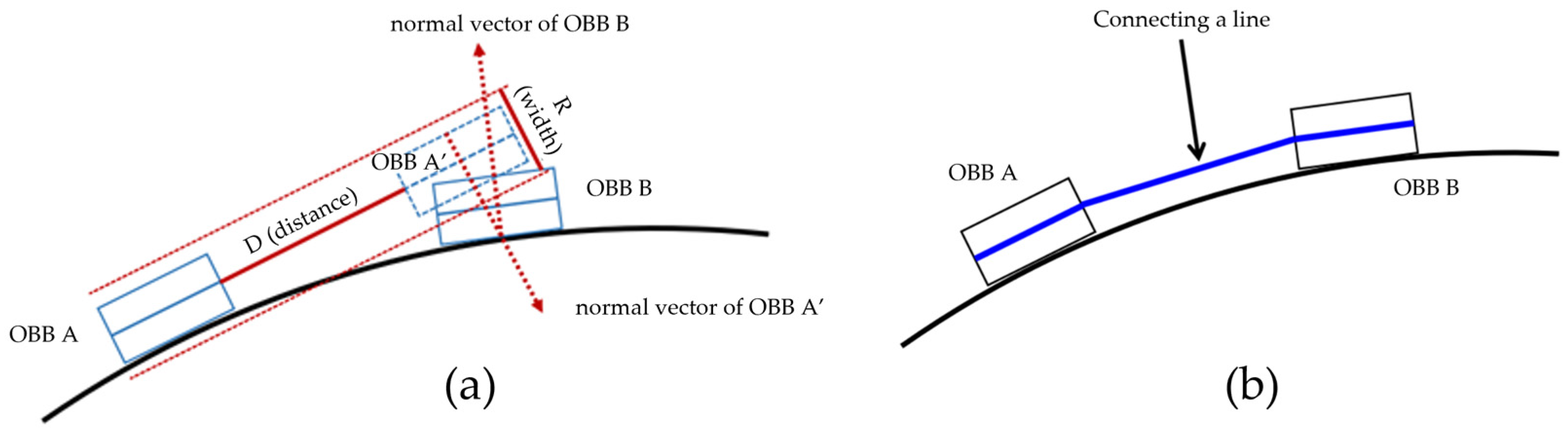
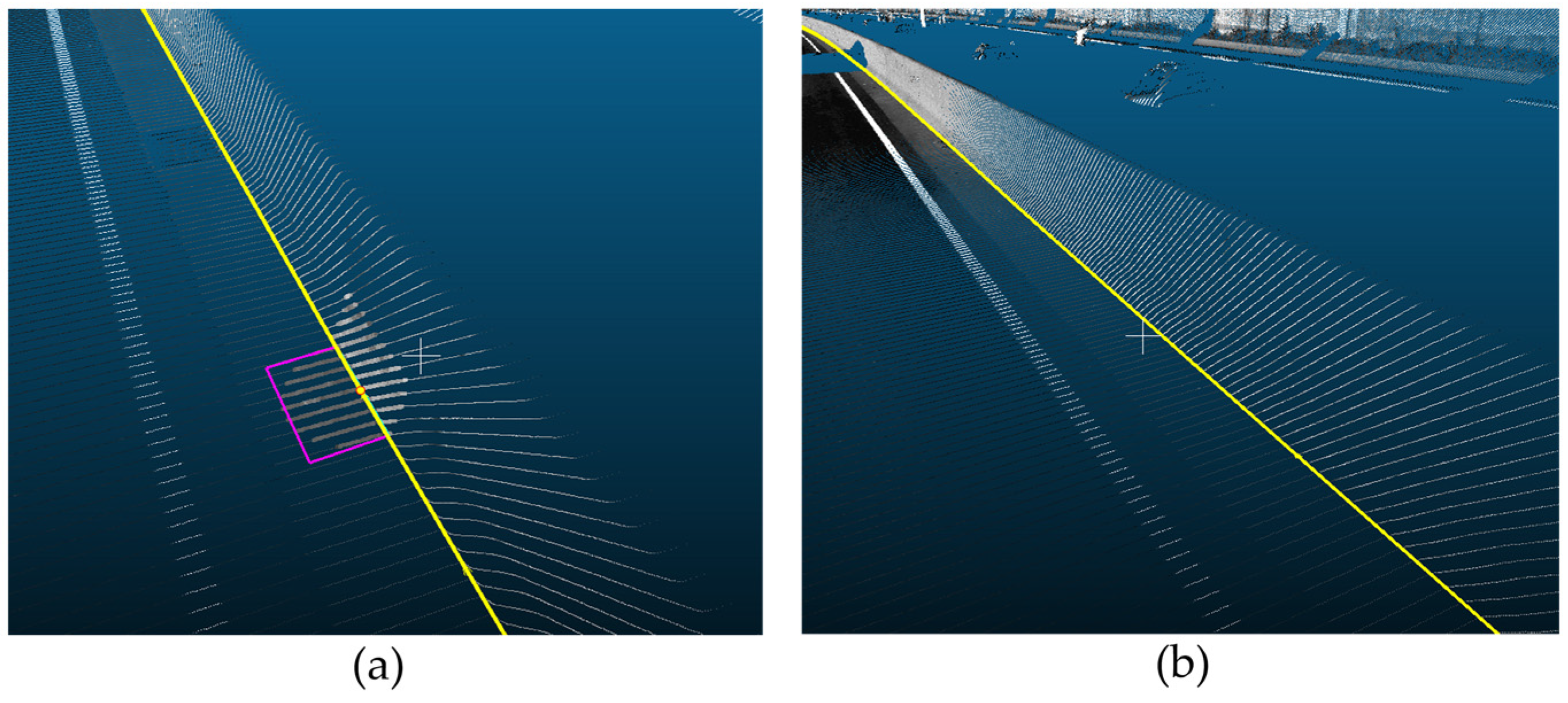
3.1. Creating Oriented Bounding Box of Road Boundaries Using Normal Vector

In many studies, a bounding box specifies spatial locations and classes (e.g., cars and trees). A bounding box is widely used in point cloud data to simplify the complex set of points as a representative box and apply collision detection [41]. Among the several types of bounding boxes, the oriented bounding box (OBB) is the smallest rectangle with an inclined axis around the object (Figure 3). In contrast, an axis-aligned bounding box (AABB) is a minimum bounding hexahedron that envelops an object and conforms to a set of fixed orthogonal axes. Owing to its simple geometry, the AABB has less memory and is tested faster (Figure 3). However, describing the directional information of a given object is difficult.

In contrast, a discrete-orientation polytope (DOP) is a bounding polyhedron defined with the k number of axes. DOP can bind the object better than AABB but requires more memory (Figure 3). Comparing these two bounding boxes, the OBB is the optimal bounding box for road marking extraction regarding memory and direction information.

To generate OBBs, it is essential to establish a set of basis axes and u- and v-axes (Figure 3). The u-axis was aligned in the direction of the OBB, which acted as a reference line for defining the OBB, and the v-axis was perpendicular to the u-axis. For the OBBs of the road boundaries, the u-axis can be extracted by identifying the boundary line of the floor plane consisting of points with a normal vector of 90°. Therefore, the u-axis can be determined with the edge of the plane, which defines the OBB of the road boundaries.

A floor plane can be generated by identifying the lowest points in the search area. Applying the search area can decrease the randomness and noise in the point cloud data. In particular, this search step determined the lowest points because the lowest point of the point clouds collected from the MMS represents the road surface. Therefore, defining the proper size and location of the search area is essential in terms of accuracy and conformity to extract the edge because it ends up being a reference line aligned with the u-axis of the OBB. The radius of the search area was set as 50 cm (Figure 4b). If it is set to a radius of 1 m, the road’s curvature is ignored; instead, a straight line is generated (Figure 4a).

The location of the search area is also associated with not only the accurate extraction of the u-axis reference line of the OBB but also the generation of the road surface. Selecting the proper location of the search area can eliminate the need to pre-process the point cloud data. To generate an accurate reference line for the OBB, the search area should be located where the following conditions should be met: first, the boundaries of the road surface are clear, the direction can be confirmed, and the data should be acquired in areas with no lost data. For example, when the position of the search area is such that the boundary is identified, as shown in Figure 5a, the reference line for creating an OBB can be extracted accurately, as shown in Figure 5b.

Moreover, it is essential to encompass both road boundary and road surface within the search area. If the search area is located outside an area not in contact with the road boundary, the edge detection causes errors, as shown in Figure 6a. Moreover, if all the portions of the search area occupied the road surface, they failed to identify the edges (Figure 6b).

The plane fitted to the lowest points is defined by calculating the normal vectors of the points. Each point has a position in the point cloud data (x, y, z). Each point is collected, which together form a group of points to represent the appearance of an object. The higher the density of the point group, the more detailed the shape that can be expressed. Moreover, the point cloud data acquired from ground MMS surveys have an average precision of 2 cm; therefore, points with 2 cm errors along the y-axis were also included to fit the plane. In point cloud data, the edge of the road plane can be extracted by calculating the normal vectors based on the coordinates of each point and fitting the points to a plane. The normal vector is perpendicular to the plane. Assuming that there are three points (P1, P2, and P3) on the plane, the normal vector (N) to the plane can be obtained by calculating the cross product of the two vectors $P2-P1$ and $P3-P1$ (Figure 7).

The normal vector is calculated with Equation (1) or Equation (2).

$$NormalVector(N)=\frac{(P2-P1)\times (P3-P1)}{|\left(P2-P1\right)\times \left(P3-P1\right)|}$$

(1)

$$NormalVector(N)=\frac{Cross(P2-P1,P3-P1)}{Length\left(\right(Cross\left(P2-P1,P3-P1\right))}$$

(2)

An algorithm to calculate a normal vector is described as Algorithm 1.

Algorithm 1: Calculating a normal vector (N)

1   Input: point p1, point p2, point p3 2   Output: normal vector N(x, y, z) 3   vector $u=p0–p1$ 4   vector $v=p0–p2$ 5 6   //Calculating a plane to find normal vector 7     vector N = crossProduct(u, v) //perform cross product of two lines on the plane 8 9    If vectorSize(N) > 0 10    m_n = normalize(N) // after normalization, assign it into a new variable m_n 11 12     $m\_d=m\_n\ast A$// the distance between the origin point and the plane 13   End 14 15  //Calculating normal vector using orientation values 16   $length=sqrt(x\ast x+y\ast y+z\ast z)$ 17   $x=x/length$ 18   $y=y/length$ 19   $z=z/length$

As mentioned above, the normal vectors of the points were calculated (Figure 8a), and points whose normal vectors were nearly 90° (approximately over 85°) were fitted to a plane by applying the k-NN clustering algorithm (Figure 8b). The boundary line is formed by connecting the edge’s endpoints where the plane from the points ends. The points on the edge of the plane were connected, creating a reference line aligned with the u-axis of the OBB (Figure 8c). This method applied the width of the OBB, which was aligned with the v-axis up to 50 cm. When the radius of the search area is 50 cm, the length of the edge can be generated to be utile 1 m. However, to create a rectangular OBB for directionality, we applied an OBB width of up to 50 cm.

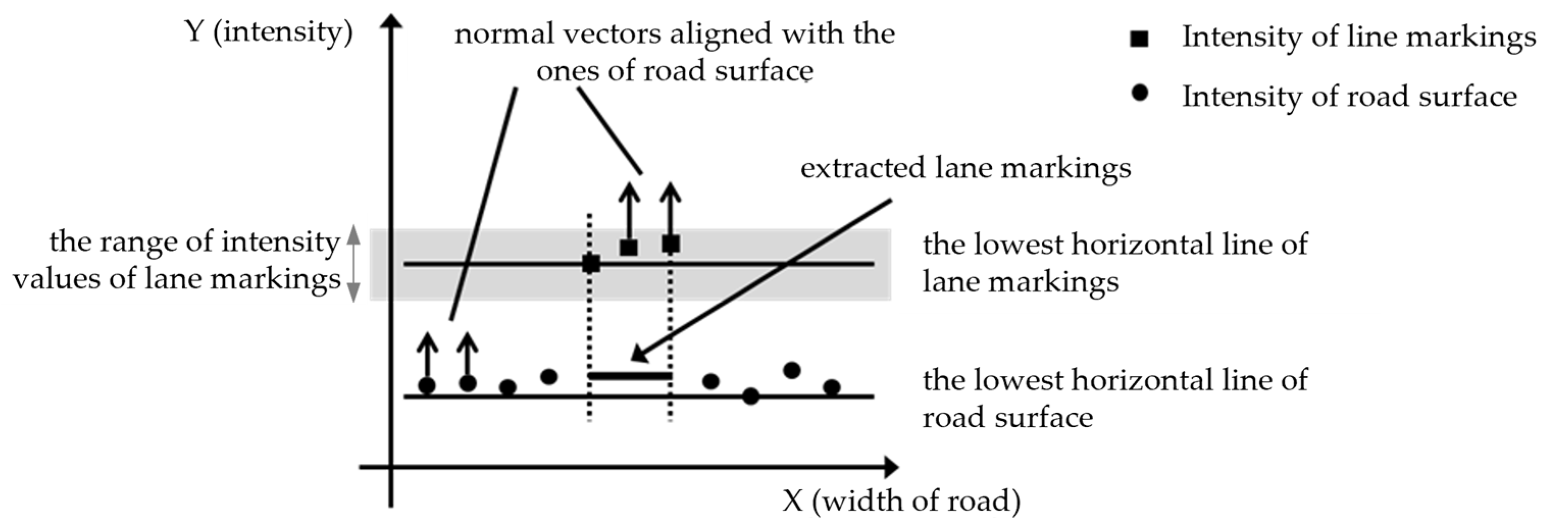
3.2. Creating Oriented Bounding Box of Edge Markings and Linear Road Markings Using Intensity Value

The point cloud data store the intensity and position values. In the point cloud data, the intensity values are stored as a short (unsigned short) type, and the value ranges from 0 to 255, where the higher the number, the higher the reflection rate. Linear road markings, which are edge and lane markings, are more likely to have a higher intensity than the surrounding environment because of the glass beads. Therefore, using intensity values, this study classifies linear road markings from point cloud data.

A range of intensity values must be established to distinguish between linear road markings. However, the intensity values are distributed depending on the measurement environment, such as weather, sunlight, and shadows. This means the intensity distribution can differ for each measurement even if the same area is resurveyed. Therefore, the intensity corresponding to linear road markings should be checked and set to include its value. After setting the range of intensity values that classified the linear road markings and road surfaces, the points of the extracted linear road markings were combined to determine the fitted plane (Figure 9).

Similar to the generation of the OBB of the road boundaries in the previous section, the points included in the search area are selected first. Subsequently, a reference line to generate the OBB of linear road markings was determined by connecting the endpoints of the point group included in the intensity value range. The centerline of the corresponding road markings was set as a reference line aligned with the u-axis of the OBB, and the width was defined as the width of the extracted linear road markings, which was 20 cm (Figure 10a). The search area, including the road marking areas, must be located to generate the OBB (Figure 10b). Even if the search area included the marking area, linear road markings with intensity values outside the set range cannot be detected, as shown in Figure 10c. None of the markings are identified if the search area excludes the marking area (Figure 10d).

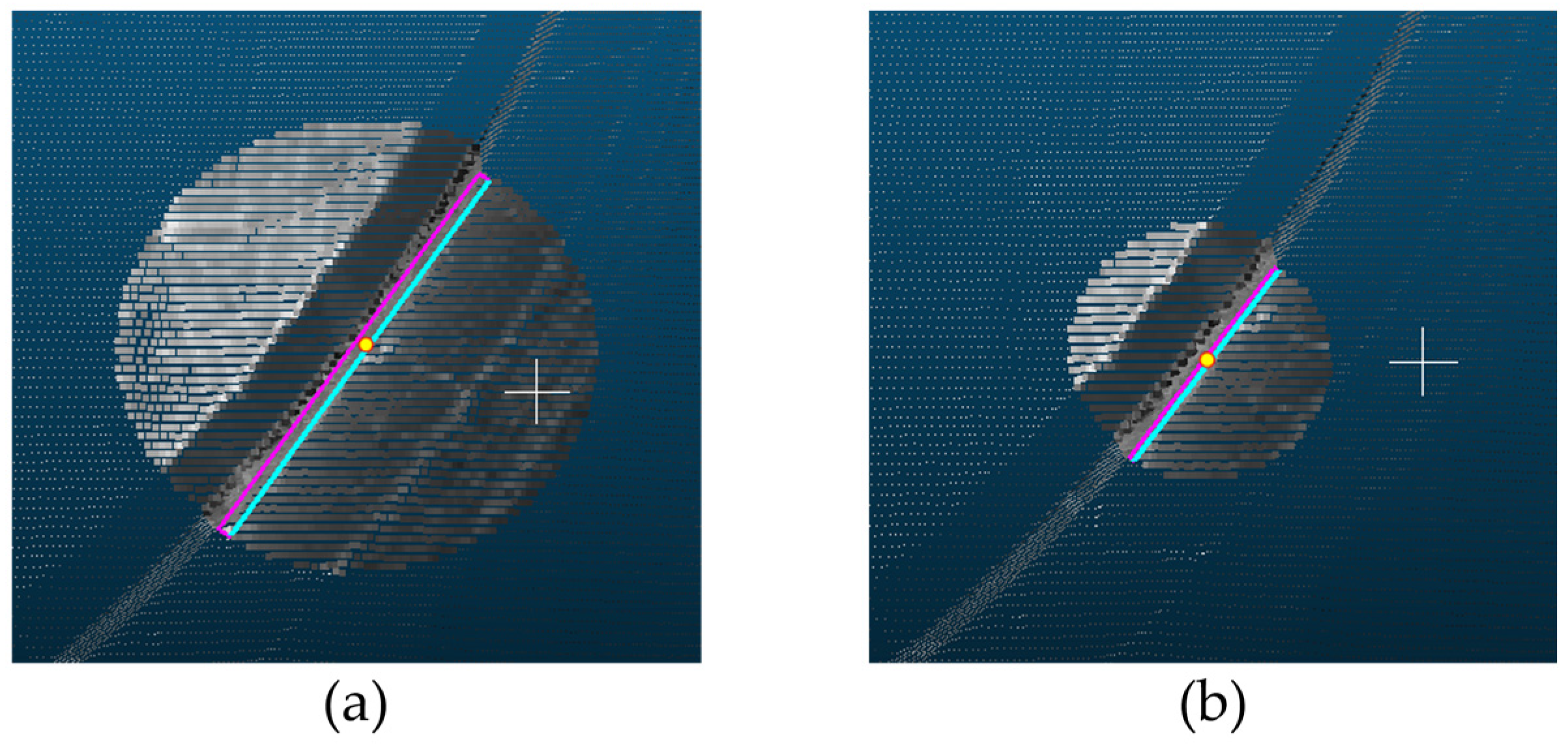
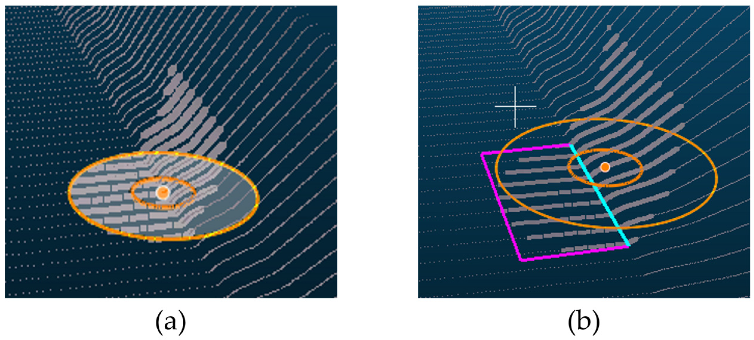
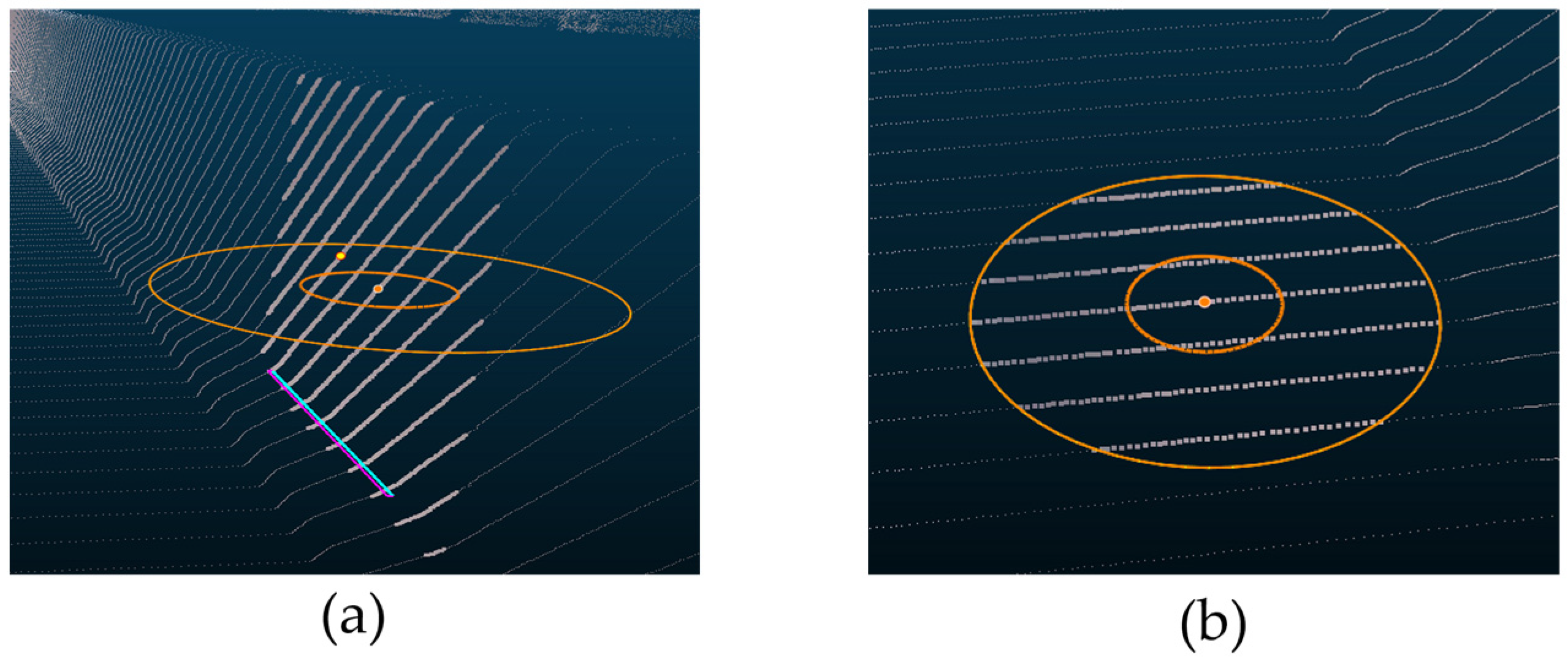
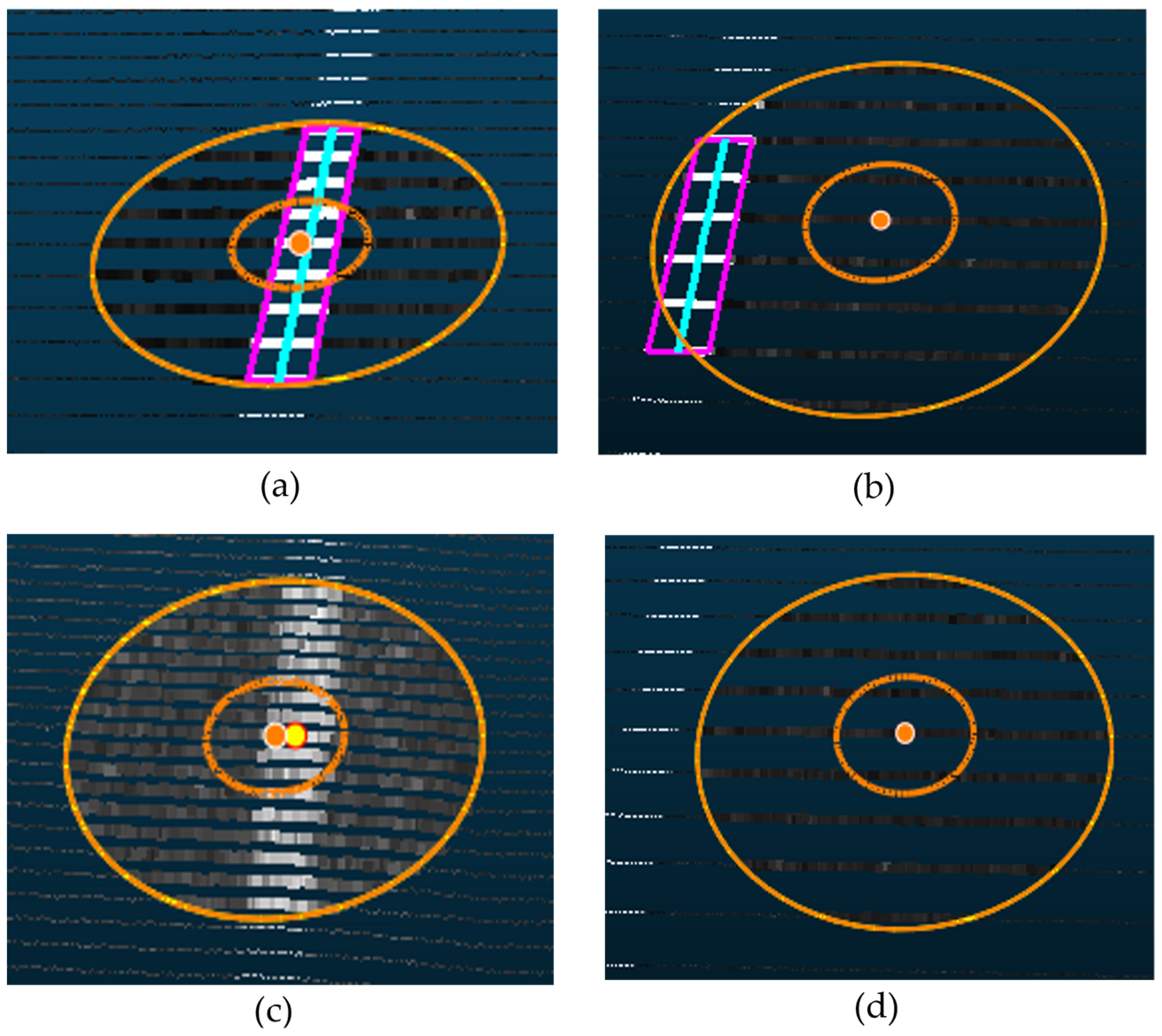
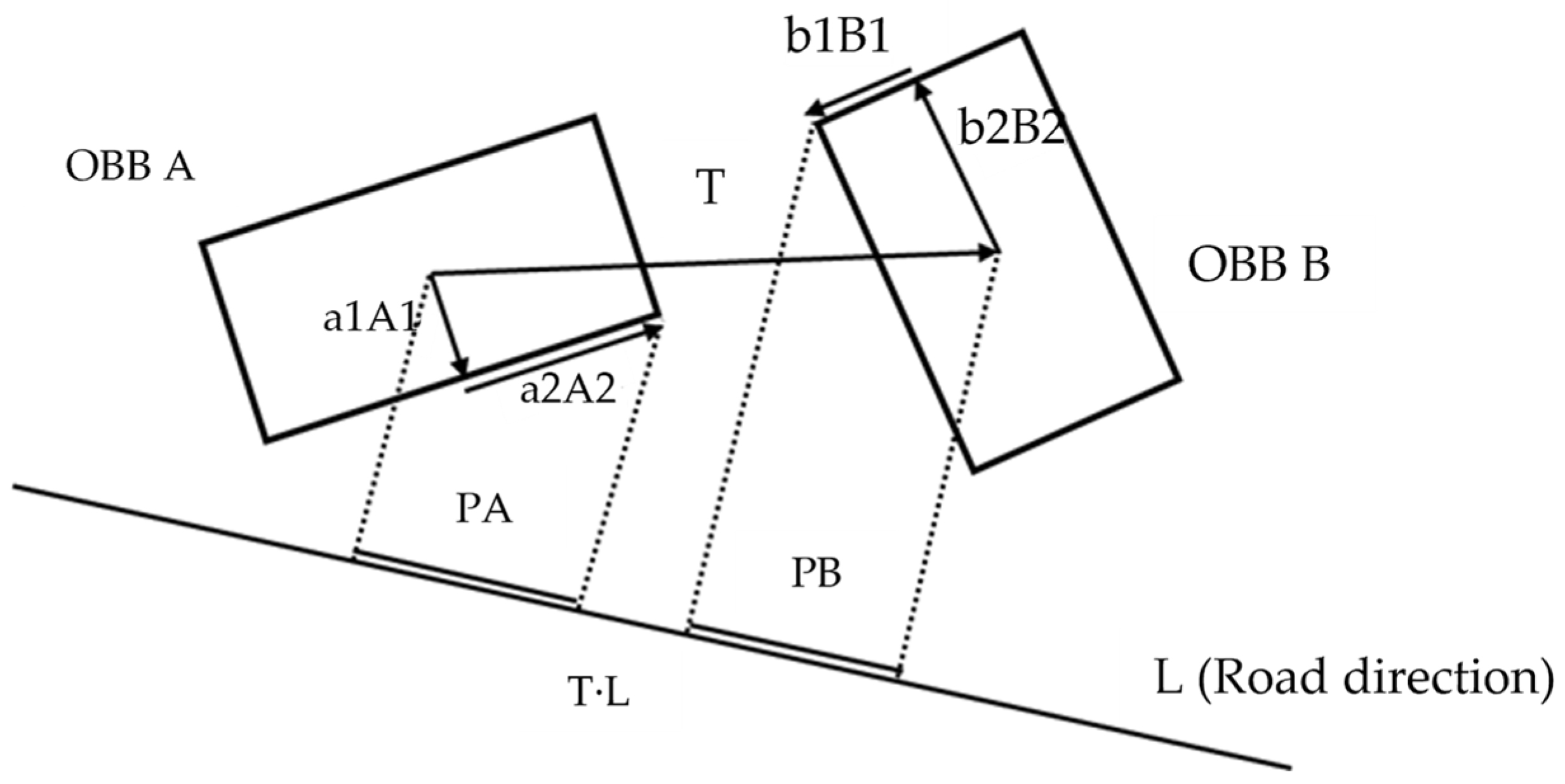
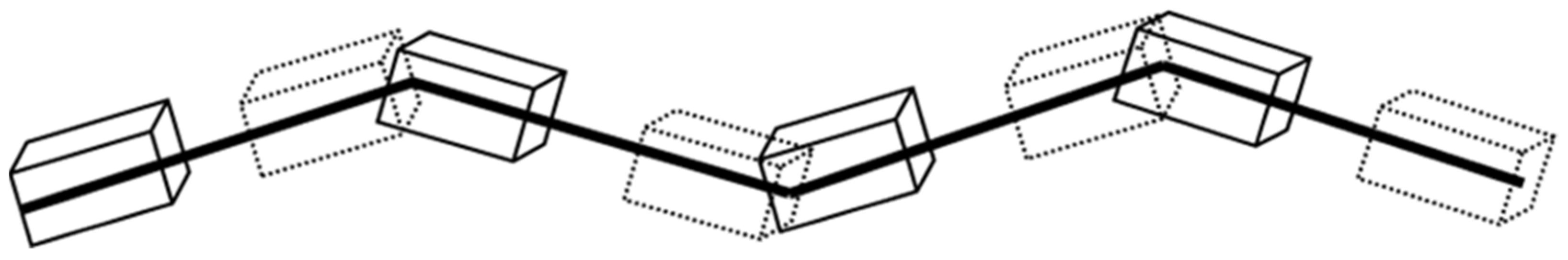
3.3. Automatic Extraction of Road Boundary and Road Markings Using Collision-Detection Algorithm

Using the generated OBBs for the road boundaries and linear road markings, linear data can be automatically extracted by setting a search radius based on these data. The OBB collision-detection algorithm is used to extract the linear data automatically. The OBB collision-detection algorithm operates based on the separating axis theorem (SAT), in which polygons are projected onto one axis and recognized as colliding objects when the projection sections overlap. In this study, the OBB was a rectangle parallel to the road-driving direction.

If an OBB rectangle is created, the OBB collision-detection algorithm connects the centerline of the conflicting OBB to build linear data based on the object. The separation axis of the figure used for applying the OBB collision-detection algorithm should apply a normal vector from the reference axis. In this study, the direction of the road was defined as the reference axis for extracting the road boundaries and lanes. If the road direction was set to that of the separation axis, the following process calculated the collision. The normal vector of the reference axis was used to check for collisions (Zhang et al. (2019) [30]), as shown in Figure 11: if the distance between the center point of $OBBA$ and that of $OBBB$ is defined as $T$, $T$ is a vector with directionality. The value projected from the vector with directionality becomes $T·L$ (Figure 11). In addition, if the sum of the length of $PA$ projecting the longest point from the center point of $A$ to the direction of $B$ and the length of $PB$ projecting the long point from the center point of $B$ to the direction of A is greater than $T·L$, a collision has occurred (Figure 11).

The collision calculation method of the separation axis theory is defined in Equations (3)–(5):

$$PA=\left|a1A1L\right|+\left|a2A2L\right|$$

(3)

$$PA=\left|a1A1L\right|+\left|a2A2L\right|$$

(4)

$$\ni L:\left|T\times L\right|>PA+PB$$

(5)

To automatically extract the linear data, the reference data to which the first acquired OBB is applied are used to check whether a line connects forward and backward. The search method obtains the range’s start- and endpoint groups by applying a search interval. Because the road may not be horizontal, an OBB was generated by applying a height equal to the search width. Subsequently, the OBB was generated at a position corresponding to the forward and backward intervals. The OBB is connected to the corresponding OBB and reference data to connect the lines (Figure 12).

The pseudocode for the OBB collision-detection algorithm is as follows (Algorithm 2).

Algorithm 2: Overlapped OBB collision detection algorithm

1   function OverlapOBB ($\mathrm{O}\mathrm{B}\mathrm{B}A,\mathrm{O}\mathrm{B}\mathrm{B}B,\mathrm{n}\mathrm{o}\mathrm{r}\mathrm{m}\mathrm{a}\mathrm{l}\mathrm{V}\mathrm{e}\mathrm{c}\mathrm{t}\mathrm{o}\mathrm{r}V$): 2     for($i$ = 0; $i$ < $A.AllNodes$; $i++$): 3        $t=$ $A.V.Node\left[i\right]$ 4        $dMin$ = t 5          $dMax$ = t 6        // calculate the length between nodes 7        for (c = 1; c < $A.V.Nodes\left[i\right]$; c++): 8             $t$ = ($t$ + $A.V.Nodes\left[i\right]$) / 2 9             if ($t<dMin$): 10               $dMin=t$ 11             elseif ($t>dMax$): 12               $dMax=t$ 13             // check the length is in the range between dMin and dMax 14        if (($dMin>t\left)\right|\left|\right(dMax<t$)): 15                // The OBBs are not overlapped 16                return false 17        return true

The two elements of the initial settings were search intervals: search length and width. The proper setting of search intervals is essential because the proposed automatic extraction method can be applied to straight and curved roads. Therefore, the search length and width are the parameters of this method based on the conditions of the applied site, which should be applied differently depending on the shape of the road. For example, highly accurate linear data can be extracted from straight roads by increasing the search length and applying a narrow search width. The search length should be shortened for curved roads, and a wide search width should be applied. The procedure for generating linear data by applying the OBB collision-detection algorithm is shown in Figure 13.

$OBBA$ generated as reference data was moved using a search length based on the road direction to generate $OBBA\prime$ in the corresponding direction. The normal vector is then obtained from the direction of $OBBA\prime$, and the point at which the normal vector meets the direction of the road is obtained. After that, the normal vector is calculated at the corresponding point, and $OBBB$ is generated based on the road direction and normal vector. Subsequently, $OBBA\prime$ and $OBBB$ were inspected for collisions using the OBB collision-detection algorithm (Figure 14a). Collision detection was performed in the above order. When a collision was detected, linear data were generated by connecting the center points of $OBBA$ and $OBBB$ (Figure 14b).

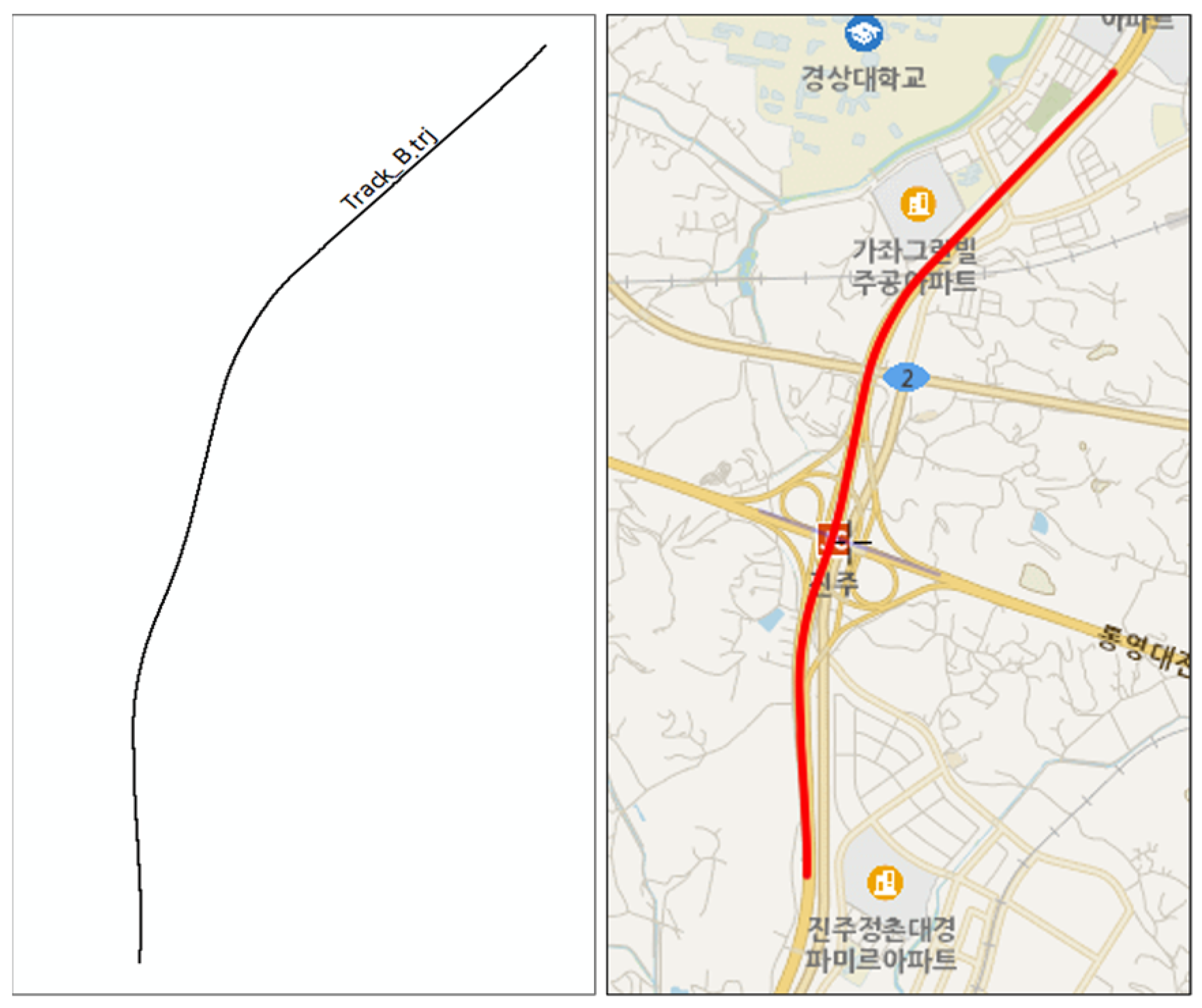
4. Experiments on Automatically Extracting Road Boundaries and Linear Road Markings

An experiment was conducted using the proposed method. First, this experimental setup sets a search area and generates an OBB for road boundaries and linear road markings. We then determined the search distance and width to detect collisions between OBBs and automatically extracted road boundaries and linear road markings on the pavement.

The experiment used a CPU with an i7 processor, 16 gigabytes of main memory, 2 gigabytes of graphics memory, and HDD storage. The operating system was 64-bit Windows 11. In addition, VC++ (2009) was used as the development language for point group data hierarchical structuring and point group extraction functions, and libLAS was used to read and write the LAS files.

The experimental subject for automatic road linear data extraction was selected as a point group file, 3223.50 m (3.22 km) of the Namhae Expressway in Korea, passing through Jinju JC (Figure 15). This experiment aims to automatically extract all road boundaries and lane markings on road pavements.

5. Results and Discussion

This section describes the experimental results. We calculated the horizontal accuracy using manually digitized MMS point cloud data to verify the method and discuss the results.

5.1. Result of the Experiments of Automatically Extracting Road Boundaries and Linear Road Markings

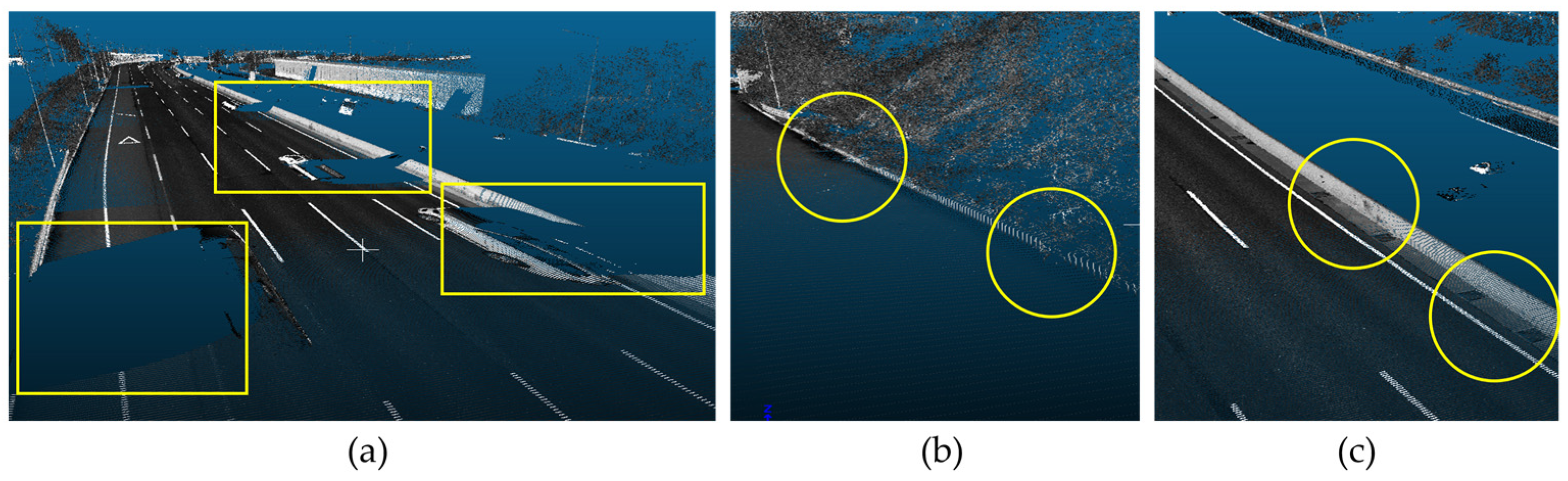
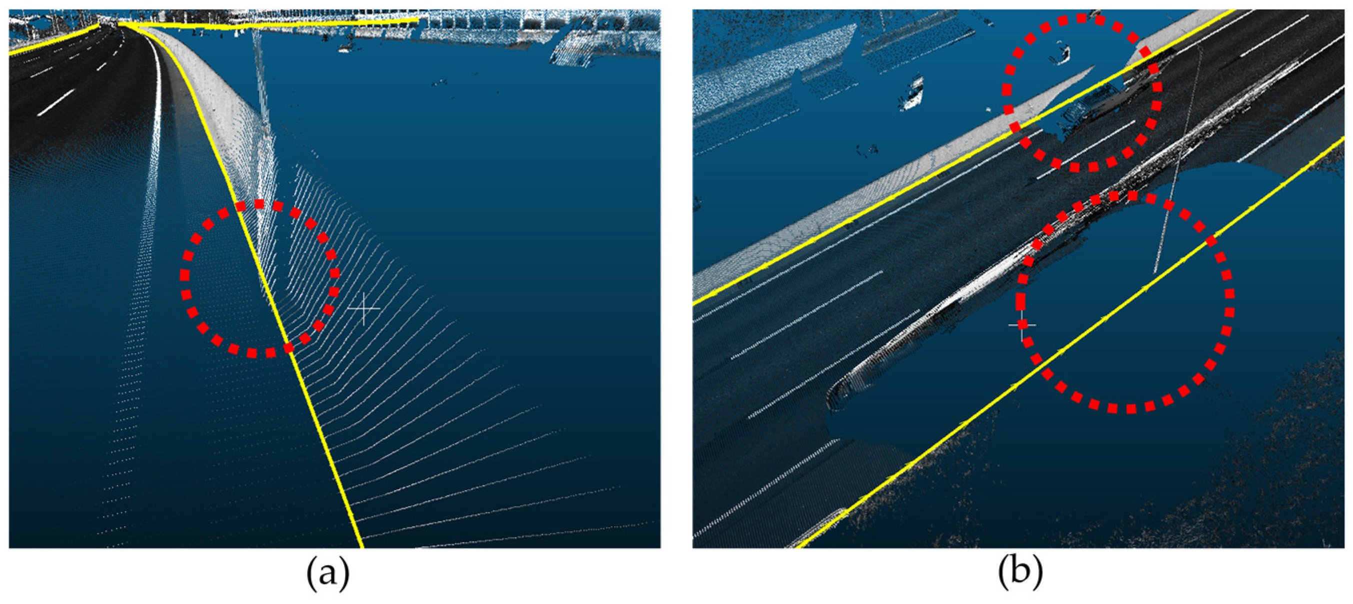
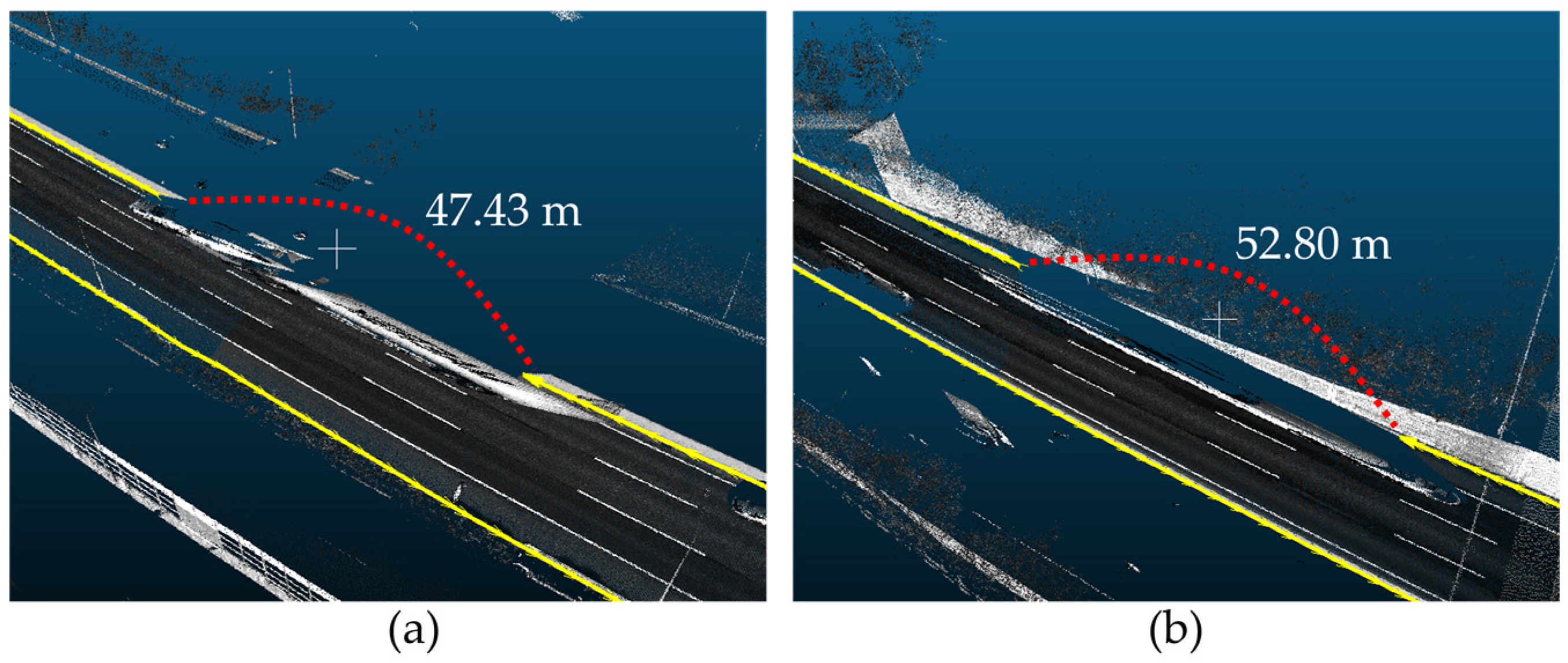
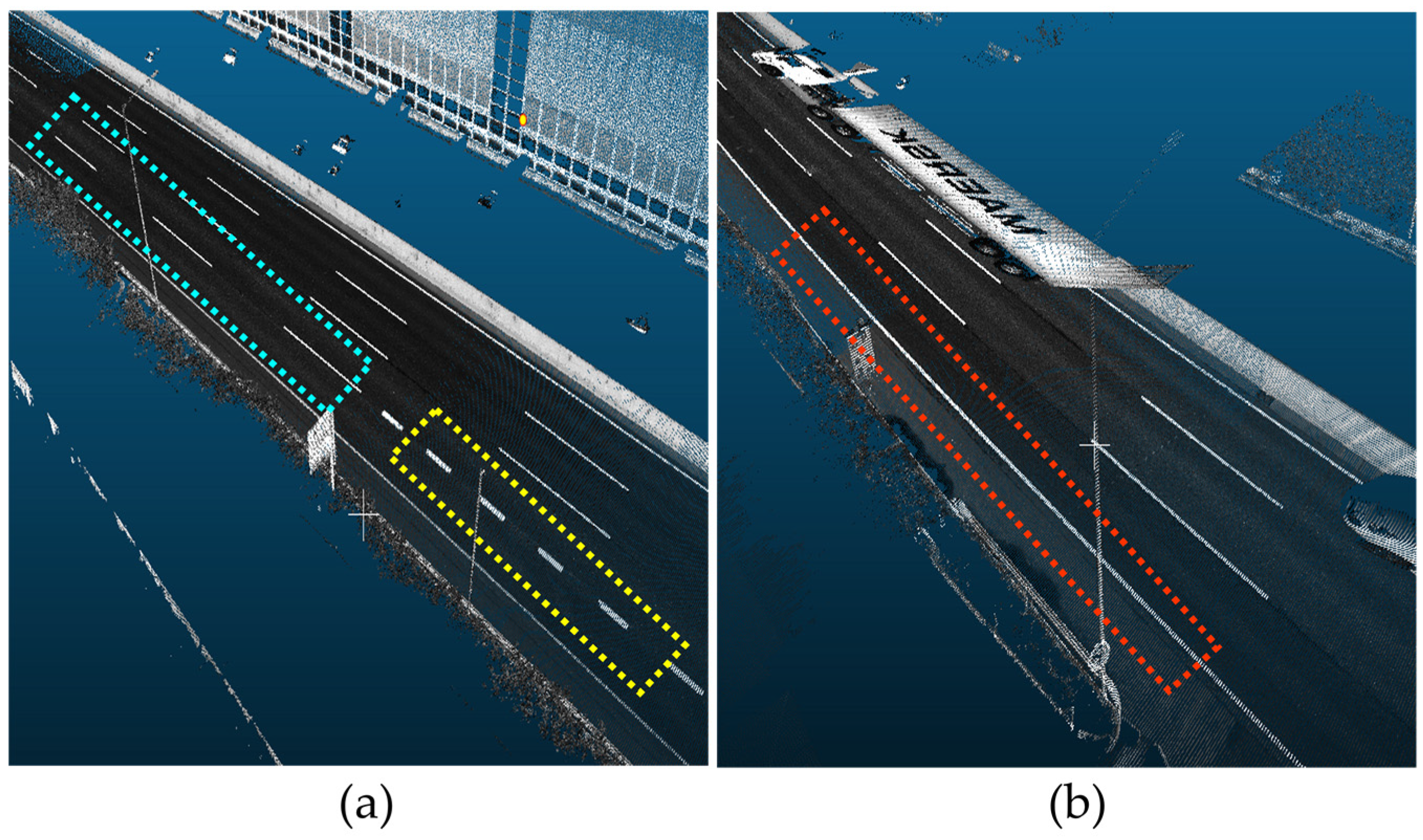
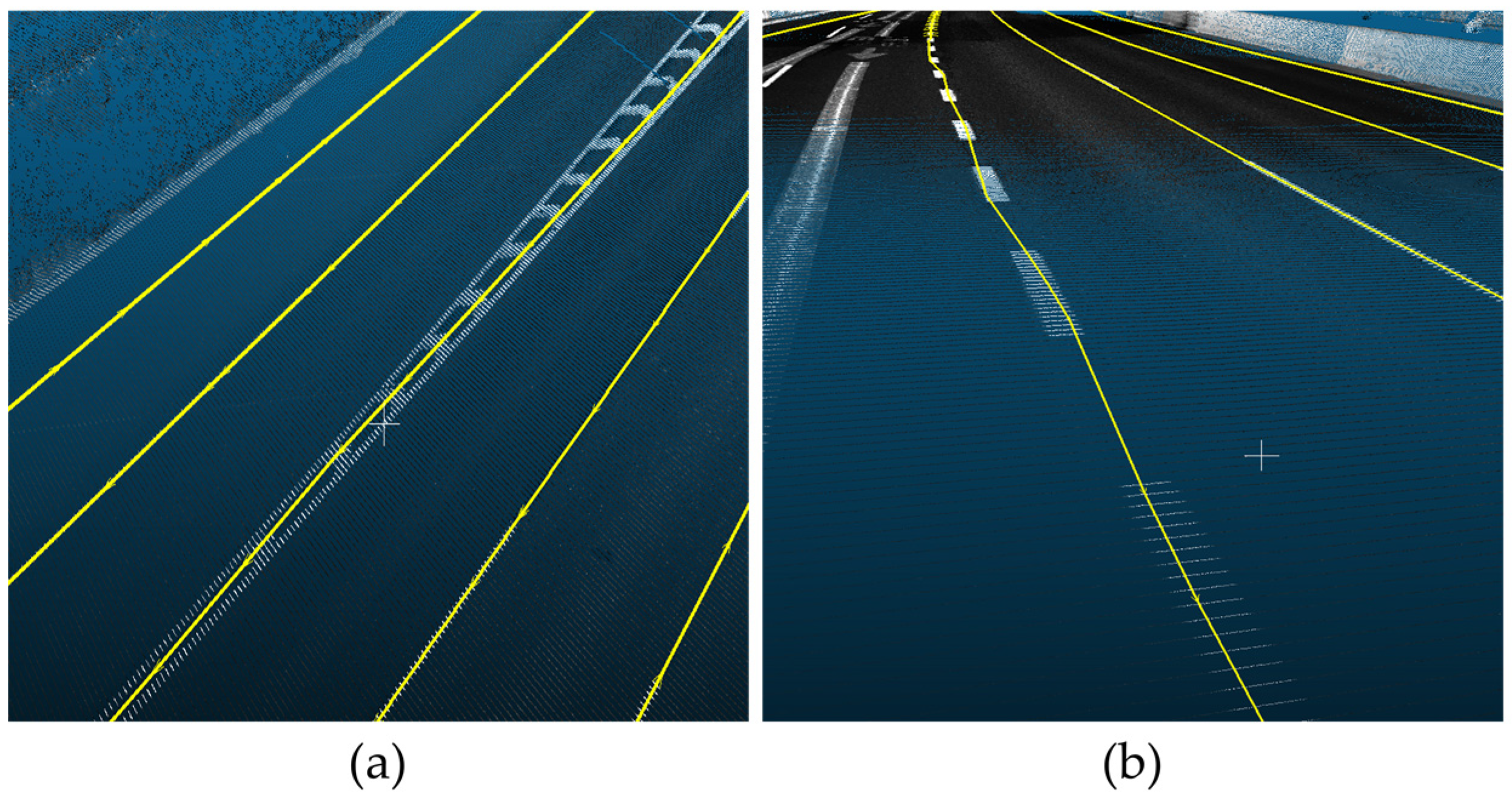
5.1.1. Result of Automatic Road Boundaries Extraction

To generate the reference line for the OBB, the search length and width should be determined based on the road conditions in the case area. The more curved the segments of the road boundaries the case area has, the shorter the search length, and the longer the search width, the more effective the collision with OBBs.

In our experiments, there were several occluded areas owing to surrounding vehicles (Figure 16a), and some factors hindered the generation of the reference line, such as bushes (Figure 16b) and rainwater basins (Figure 16c).

The following are the results of the experiments to verify the proposed method to automatically extract the right- and left-hand road boundaries based on driving direction. For right road boundary extraction, the search length and width are set to 5 m and 8 cm, respectively (expanded by 8 cm on each side of the width of the generated OBB). The search process was repeated five times to calculate the missing data from the surrounding data.

Table 1. Results of automatic extraction of right-hand road boundaries (search length: 5 m, search width: 8 cm, performed five times).

Numbers of Trials	The Length of Extracted Linear Road Markings (m)	The Length of Failure Section (m)
1	815.39	47.43
2	872.78	-
3	226.32	-
4	1186.24	-
5	51.89	-
Sum	3152.62	47.43

shows the results of the automatic extraction of the right-side road boundary data. As a result, the total length of the extracted data was 3152.62 m, and the 47.43 m occluded area could not be captured (Table 1).

For the left-side road boundaries, the search length and width were set to 4 m and 1 cm, respectively (expanded by 1 cm on each side of the width of the generated OBB). This is because, as shown in Figure 15, the case area is slightly curved to the right. Therefore, to increase the automatically extracted area, the search length for the left-side road boundaries should be shorter than that for the right-side road boundaries. Moreover, owing to superelevation, a transverse slope along the road, increasing the outer edge of the road concerning the inner edge to decrease the chances of vehicles overturning, many rainwater basins were distributed on the left. This creates more noise on the left and right road boundaries; therefore, we applied a narrow search width. The search process was repeated five times, and the extraction was finalized four times. The total length of the extracted left road boundary is 3124.13 m, but the method failed to extract 52.80 m due to occlusion (

Table 2. Results of automatic extraction of left-hand road boundary data (search length: 4 m, search width: 1 cm, performed four times).

Numbers of Trials	The Length of Extracted Linear Road Markings (m)	The Length of Failure Section (m)
1	1176.22	52.80
2	771.20	-
3	405.30	-
4	771.41	-
Sum	3124.13	52.80

).

Excluding the failed automatic extraction points owing to the occluded area at the right boundary, the length of the extraction error at 3152 m was 156.78 m, which was a success rate of 98.52%. Excluding the failed automatic extraction points due to occlusions at the left boundary line, the length of the extraction error at 3124 m was 270.37 m, a 95.03% success rate (

Table 3. The overall result of automatic road boundary extraction.

Items	Length of Correct Extraction (m)	Length of Extraction Error (m)	Total Length (m)	Success Rate of Extraction (%)	Error Ratio of Extraction (%)
right road boundaries	2995.84	156.78	3,152,62	95.03	4.97
left road boundaries	2853.76	270.37	3,124,13	91.35	8.56

).

In summary, four cases of automatic road boundary extraction were successful. Results show that the road boundaries were accurately extracted in areas where a reference line for the OBB was correctly generated (Figure 17a) or where the road boundary was identified (Figure 17b).

In addition, a repetitive search enables the extraction of road boundaries in areas with short-distance occlusions by ignoring them through repeated searches, shown in Figure 18a. Moreover, as Figure 18b shows, connecting a line between the OBBs can ignore fine noise and extract the road boundaries.

However, there are two types of errors in the automatic extraction of road boundaries. First, the extraction failed in occluded areas that exceeded the search length and width (Figure 19).

Moreover, results confirmed that if two reference data values were extracted owing to uneven road conditions (Figure 20a,b), there would be a discrepancy between the automatically extracted road boundary data and the ground truth, as shown in Figure 20c.

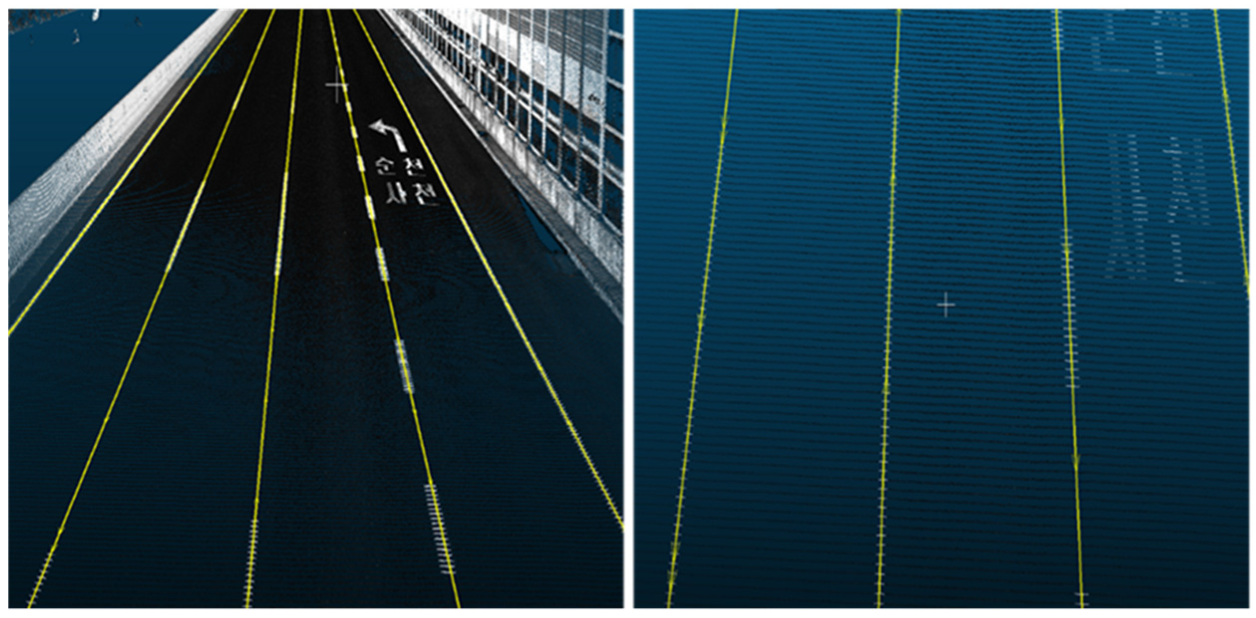
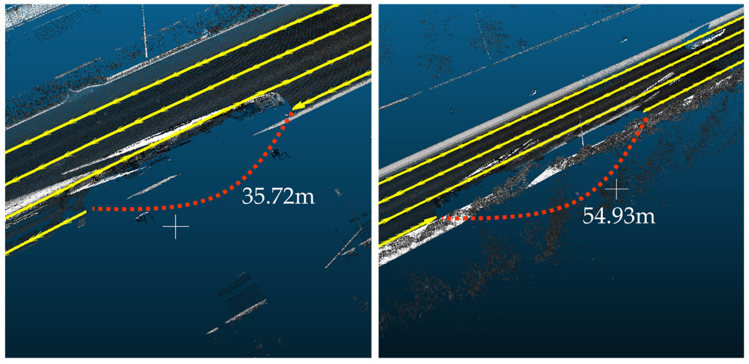
5.1.2. Result of Automatic Linear Road Markings Extraction

Dotted or solid lines indicate linear road markings containing edges and lane markings. The edge markings are primarily represented with solid lines (Figure 21a), and the lane markings are indicated with dotted lines (Figure 21b). The data in our case area, a three-lane road, comprise complex road markings of various lengths and widths. Therefore, to detect collisions with OBBs and continuously extract linear road markings, we assigned different search lengths and widths to each type of marking (Figure 21).

Overall, the intensity values of the road markings were high, but some were relatively low and hindered by intersections. Therefore, after examining the overall distribution of the intensity values, we considered the range of intensity values for road markings between 180 and 255.

Table 4. Results of automatically extracting lane markings (intensity value range: 180~255, search length: 1~8 m, search width: 4~8 cm, performed five times on lane 3).

Item	The Length of Extracted Lane Markings (m)	The Length of Failure Section (m)
Lane 1	3200.54	-
Lane 2	3198.11	-
Lane 3	1170.60 240.28 720.77 892.35 153.28	54.93 35.72
Sum	3114.28	90.65

presents the results of the automatic extraction of lane markings. The search length and width were constant in lanes 1 and 2 because they did not have occlusions. However, in the case of lane 3, different search lengths and widths were applied in each of the five trials because they had different markings, solid lines, two types of dotted lines with different intervals, and some occluded areas.

Table 5. Results of automatically extracting edge markings (intensity value range: 180~255, search length: 8 m, search width: 8 cm, performed four times on center edge markings).

Item	The Length of Extracted Edge Markings (m)	The Length of Failure Section (m)
center edge markings	1575.97 605.42 155.20 837.51	25.13
edge markings	1151.82	-

shows the results of the automatic extraction of edge markings. The search length and width for edge markings are set to 8 m and 8 cm, respectively, for automatic extraction. The target road was connected to a highway exit, where lanes were reduced from four to three. These three lanes were divided with a combination of dotted and solid lines, and the fourth lane was connected to the exit; thus, it existed for only approximately 1 km (Table 5). The reason for this failure is occlusion.

The results of the automatic extraction of markings are shown in Figure 22. Overall, the edge and lane markings were extracted within the marking areas because the case site had distinctive markings.

By comparing the results with the photographs taken at the measuring point, the extracted edge and lane markings were aligned and corresponded to the ground truth (Figure 23).

However, results show that the primary sources of errors were occlusion, locational properties, and intensity values. The automatic extraction method could extract edge marking data when the range of the occluded area was outside 25 m despite five repetitions (Figure 24).

Moreover, automatic extraction errors occurred at locations where the number of lanes changed (Figure 25a). Because the locations had a complex form of lanes, a center calculation error of the lane occurred. In addition, the locations where the intensity value was unclear generated curved lines (Figure 25b).

The overall results of the automatic extraction of the edge and lane markings are listed in

Table 6. Comparison of results of automatic edge marking and lane markings extraction.

Item	The Length of Extracted Markings (m)	Success Rate of Extraction (%)	The Length of Failed Extraction (m)	The Ratio of Extraction Error (%)
Edge markings	4301.62	99.44	24.30	0.56
Lane markings	9314.05	97.91	198.88	2.09

. One criterion for determining the success or failure of extraction is whether the extracted line is generated within the marking areas. For edge markings, the length of the extraction error was 24.30 m at 4325.92 m, excluding the automatic extraction failure point, which is a 99.44% accuracy rate. For dotted lines, the length of the extraction error was 198.88 m at 9512.98 m, excluding the automatic extraction failure points of occluded areas, resulting in a 97.91% success rate (Table 6).

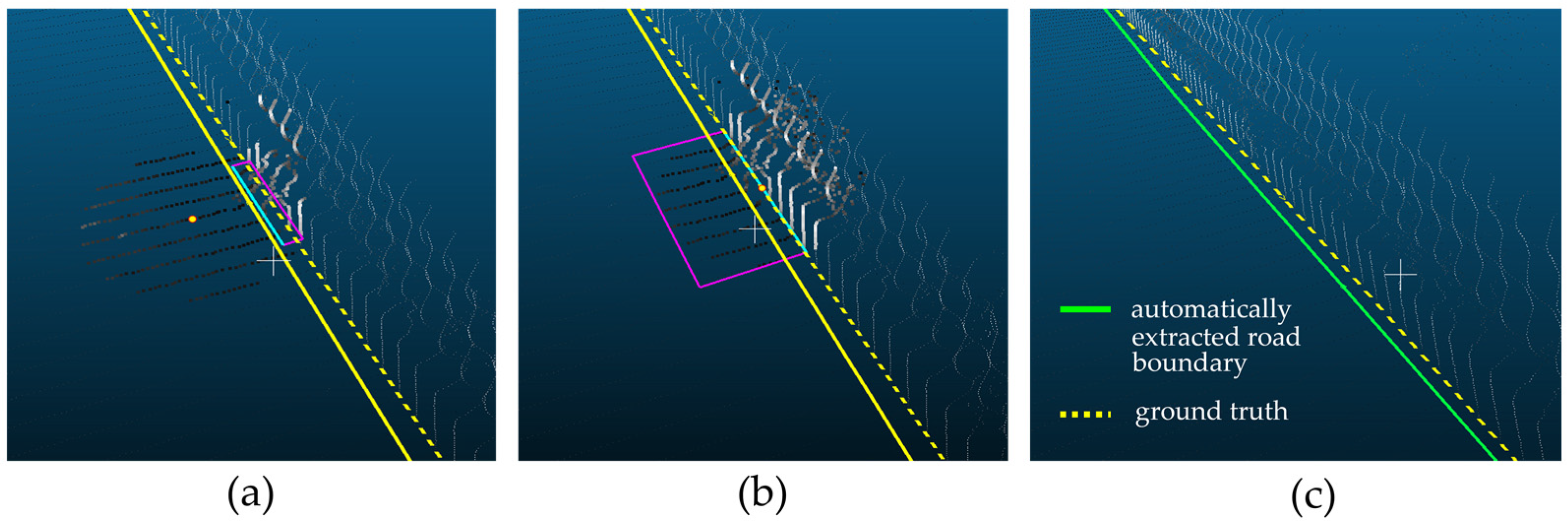
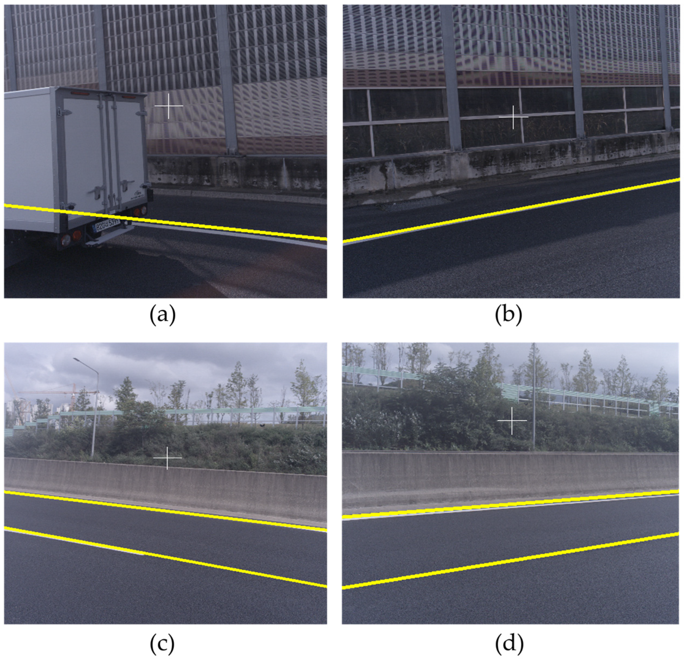
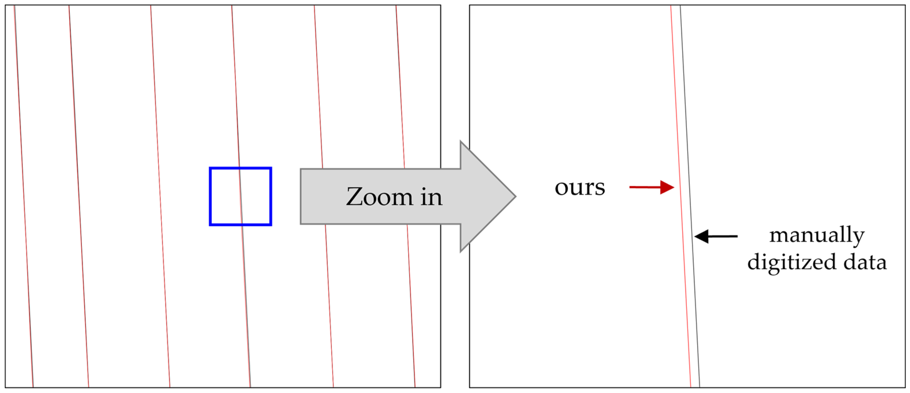
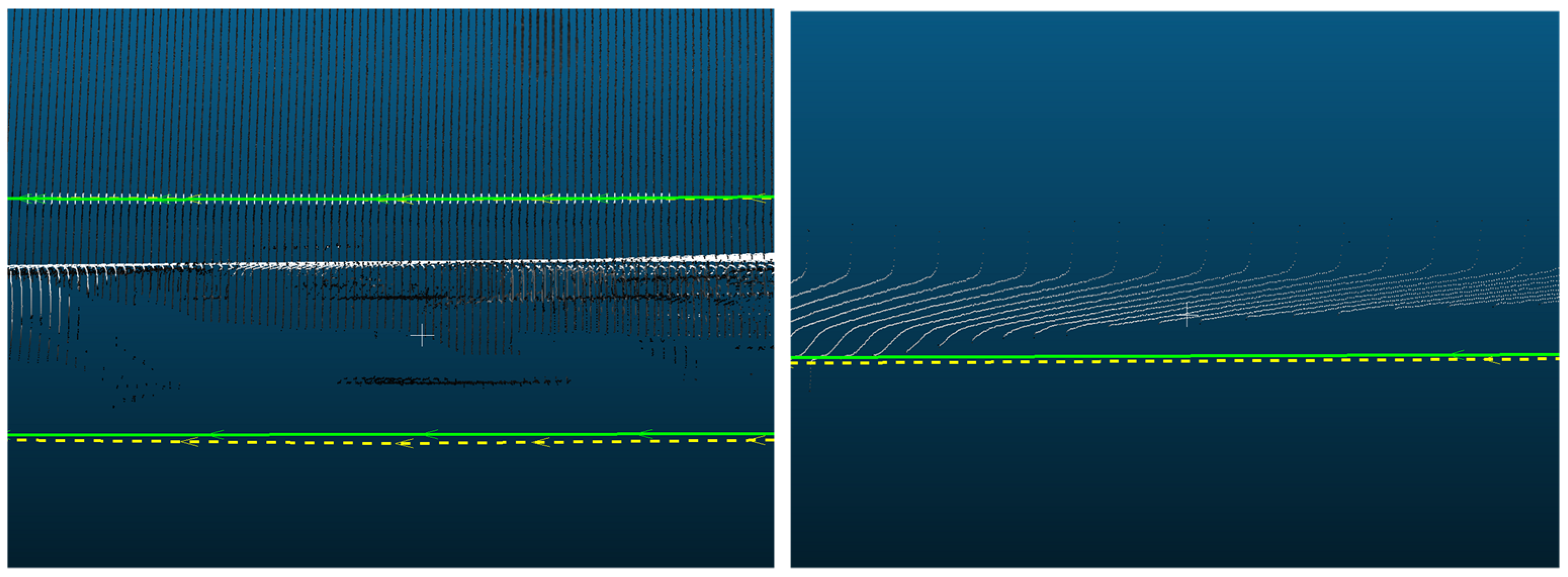
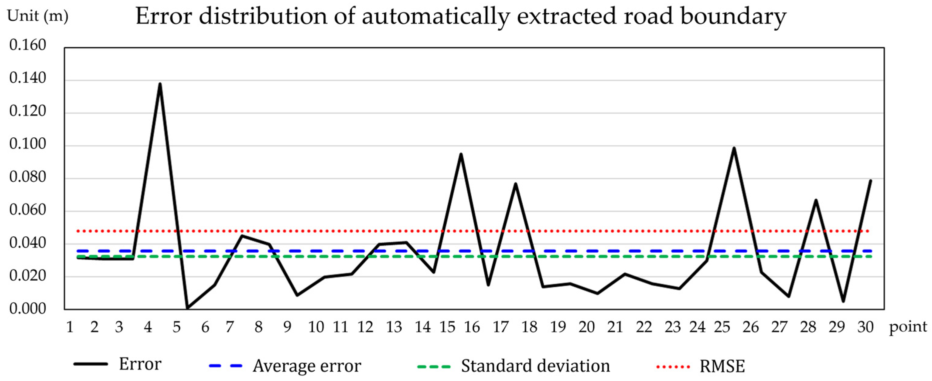
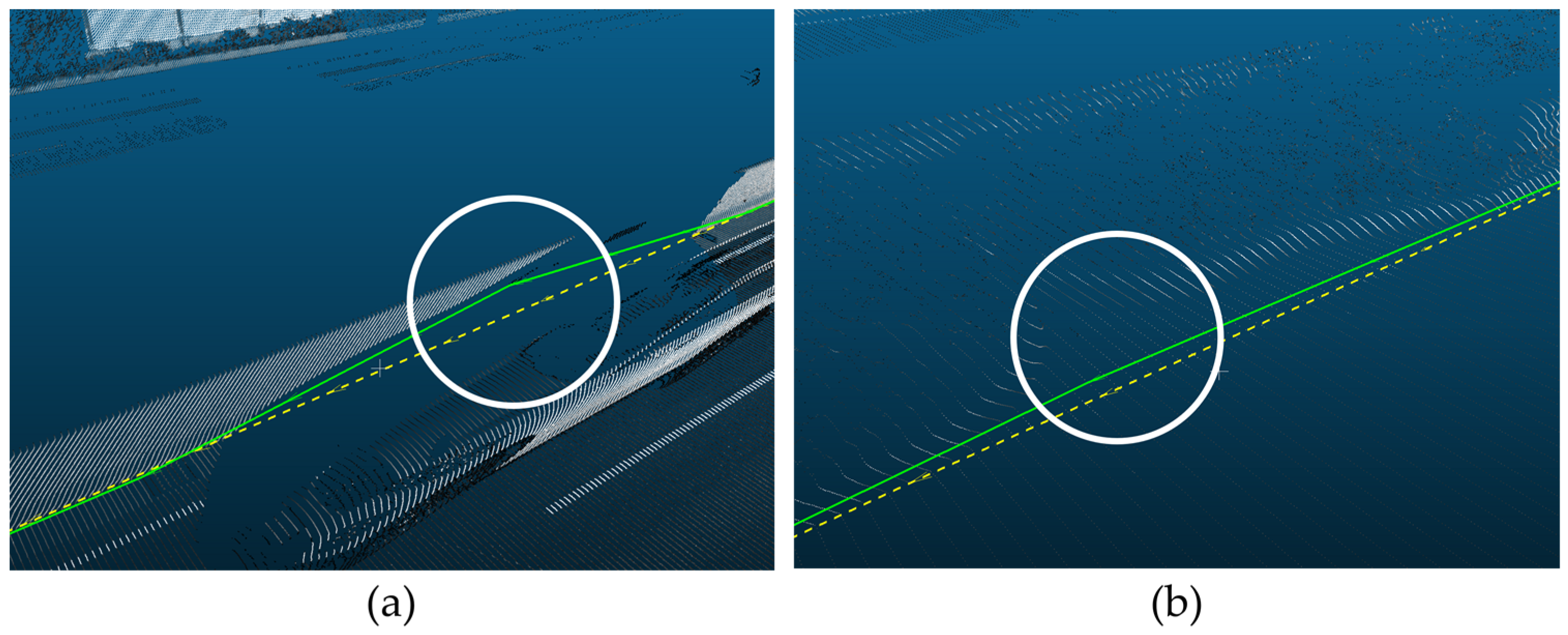
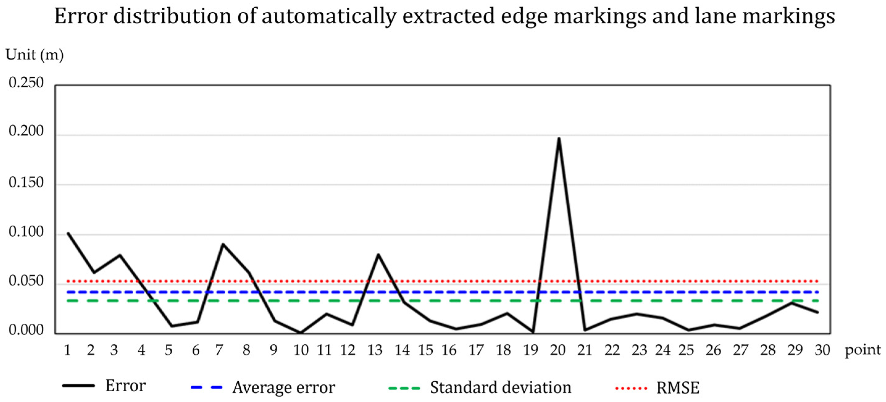
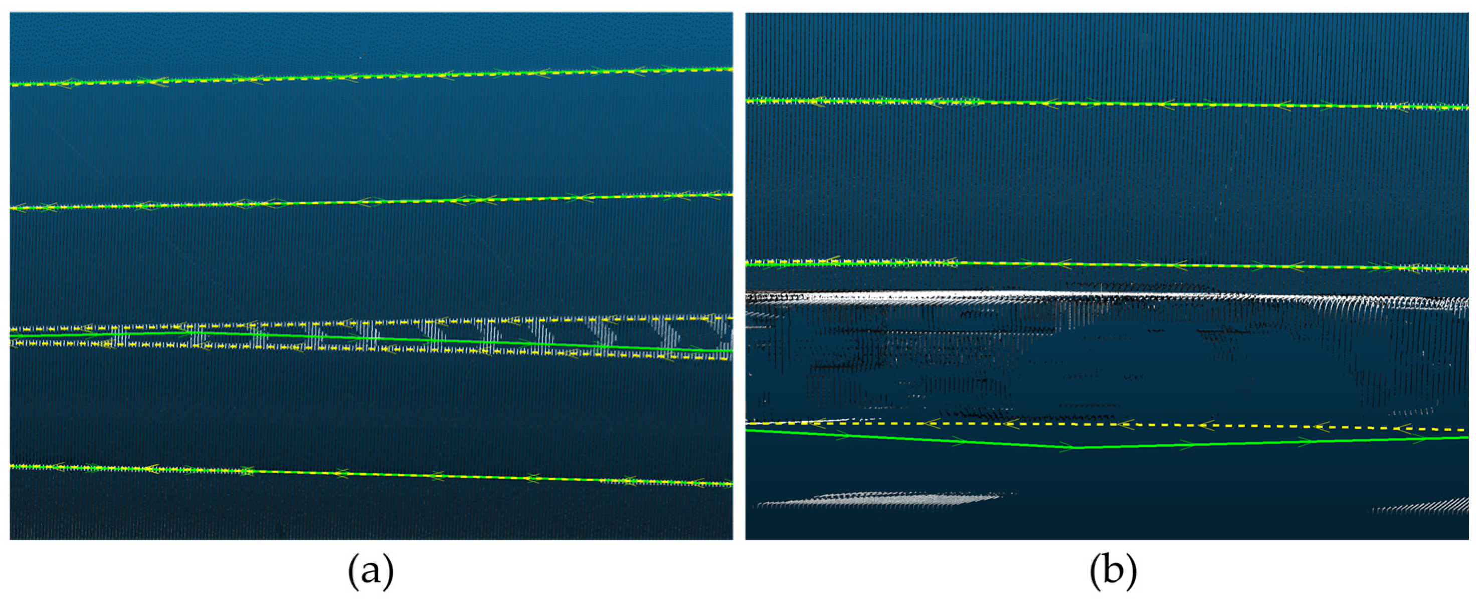
5.2. Comparing Positional Accuracy between Automatically Extracted Data and Manually Digitized Data and Verifying the Method

This section discusses the assessment of the horizontal position accuracy of the automatically extracted linear data by comparing them with manually digitized data for verifying the results of the proposed method. We evaluated horizontal positional accuracy because the manually digitized data were constructed at a lower level than ours. The comparative data were manually digitized road data provided by the National Geographic Institute and considered ground truth data. The error values were calculated by overlapping the two layers and computing the separation distance between the lines using the QGIS (Figure 26).

For the total road length of approximately 3 km, we measured the separation distances of the road boundaries and linear road markings in 100-meter intervals for 30 points and calculated the minimum, maximum, mean, standard deviation, and Root Mean Square Error (RMSE) values.

Table 7. The statistical summary of horizontal position error of automatically extracted road boundaries, linear road markings, and manually digitized data.

Item	Min (m)	Max (m)	Mean (m)	Standard Deviation (m)	RMSE (m)
Error in road boundary	0.001	0.138	0.036	0.035	0.048
Error in edge markings and lane markings	0.001	0.197	0.034	0.042	0.053

presents a statistical summary of the horizontal accuracy of the automatically extracted road boundaries and the extracted linear road, edge, and lane markings. According to Table 7, the RMSE for the extracted road boundaries is $+4.8$ cm, and the RMSE for linear road markings is $+5.3$ cm, which can be considered a favorable performance (Figure 27).

Figure 28 shows the distribution of the error values of the automatically extracted road boundary data for every 30 points.

To identify the reason for the high error level, we inspected points with errors greater than the RMSE. These points generally indicate some reasons for this. The main reason for this was occlusion. As shown in Figure 29a, the extracted line is generated using a randomly occluded area. Another reason was the noise at the boundary (Figure 29b).

Similarly, Figure 30 shows the distribution of the error values of the automatically extracted linear road marking data for every 30 points.

At some points, the error was larger than the other methods. The main reason for the high error values is that the points were areas where a lane was separated into two, which changed the number of lanes (Figure 31a). In addition, the occlusion caused errors because missing data in the occluded area generated randomly estimated points (Figure 31b).

6. Conclusions

This study developed a method to automatically extract road boundaries, linear road markings, edge markings, and lane markings from MMS point cloud data. This proposed method generated reference lines for road boundaries and linear road markings to create OBBs. The reference lines for the road boundaries were extracted from the boundary of a plane by clustering points whose normal vector was approximately 90°. Reference lines for linear road markings were generated using the intensity values. After generating the OBBx, the method automatically extracts road boundaries and linear road markings by connecting their centerlines using the OBB collision-detection algorithm. This paper discusses a verification of the method by calculating the error and separation distance between our data and the manually digitized data. The results showed that the RMSE for extracted road boundaries is +4.8 cm, and for linear road markings, it is +5.3 cm. In short sections of the occluded areas, the method performed well by setting an appropriate search length and performing repetitive searches. However, occlusions, lane conditions, and noise in the data were more likely to cause errors.

Future studies are required to overcome these limitations. First, to mitigate occlusion, a predominant source of error arising from vehicular traffic and bushes, point cloud data must be collected repeatedly and merged with the collected data to minimize the extent of occluded regions. Second, when determining the threshold of the intensity value, the intensity values, ranging from 0 to 255, differ depending on the weather. For example, on sunny days, the values of road markings often exceed 200, whereas under cloudy conditions, they tend to exceed 160. Consequently, this study employed a manual approach to establish a threshold value within a randomly selected area, accounting for the weather conditions on the measurement day. However, further studies are needed to refine the determination of the intensity threshold value using thresholding algorithms such as Otsu.

Moreover, the results of this method should be compared with those of existing methods. However, this study was unable to make such a comparison with existing methods for road boundaries or road markings because of challenges in accurate implementation. However, this study verifies the method by comparing the positional accuracy with manually digitized data, regarded as ground truth data.

Further studies must be conducted using noisy data. For example, producing multiple reference datasets with an expanded search range can minimize errors by extracting duplicate patterns. Moreover, subsequent research can address the limitation of occluded areas by referencing the lanes’ width and calculating the road’s rotation angle. For example, regarding road boundaries, the extraction accuracy may be improved by applying guide data, such as the road rotation angle and width of the other side. Consequently, this study enhances the efficiency of the extraction process for road boundaries and linear road markings. Traditionally, this process has necessitated manual digitization of point cloud data, which is laborious and time-consuming. The enhanced method promotes the efficient construction of high-precision maps, which can contribute to intelligent transportation and autonomic driving development. The authors also recommend an examination of possible strategies to optimize the parameters of the proposed algorithm for enhancing its robustness and applicability in various road conditions.

References

1. Fujita, Y.; Hoshino, Y.; Ogata, S.; Kobayashi, I. Attribute Assignment to Point Cloud Data and Its Usage. Glob. J. Comput. Sci. Technol. 2015, 15, 11–18. [Google Scholar]
2. Zhang, Y.; Yang, Y.; Gao, X.; Xu, L.; Liu, B.; Liang, X. Robust Extraction of Multiple-Type Support Positioning Devices in the Catenary System of Railway Dataset Based on MLS Point Clouds. IEEE Trans. Geosci. Remote Sens. 2023, 61, 5702314. [Google Scholar] [CrossRef]
3. Kang, Z.; Zhang, Q. Semi-Automatic Road Lane Marking Detection Based on Point-Cloud Data for Mapping. J. Phys. Conf. Ser. 2020, 1453, 012141. [Google Scholar] [CrossRef]
4. Lin, C.; Guo, Y.; Li, W.; Liu, H.; Wu, D. An Automatic Lane Marking Detection Method with Low-Density Roadside LiDAR Data. IEEE Sens. J. 2021, 21, 10029–10038. [Google Scholar] [CrossRef]
5. Ma, L.; Li, Y.; Li, J.; Yu, Y.; Junior, J.M.; Gonçalves, W.N.; Chapman, M.A. Capsule-Based Networks for Road Marking Extraction and Classification From Mobile LiDAR Point Clouds. IEEE Trans. Intell. Transp. Syst. 2021, 22, 1981–1995. [Google Scholar] [CrossRef]
6. Yang, R.; Li, Q.; Tan, J.; Li, S.; Chen, X. Accurate Road Marking Detection from Noisy Point Clouds Acquired by Low-Cost Mobile LiDAR Systems. ISPRS Int. J. Geo-Inf. 2020, 9, 608. [Google Scholar] [CrossRef]
7. Yao, L.; Qin, C.; Chen, Q.; Wu, H. Automatic Road Marking Extraction and Vectorization from Vehicle-Borne Laser Scanning Data. Remote Sens. 2021, 13, 2612. [Google Scholar] [CrossRef]
8. Tian, Y.; Gelernter, J.; Wang, X.; Chen, W.; Gao, J.; Zhang, Y.; Li, X. Lane Marking Detection via Deep Convolutional Neural Network. Neurocomputing 2018, 280, 46–55. [Google Scholar] [CrossRef]
9. Wen, C.; Sun, X.; Li, J.; Wang, C.; Guo, Y.; Habib, A. A Deep Learning Framework for Road Marking Extraction, Classification and Completion from Mobile Laser Scanning Point Clouds. ISPRS J. Photogramm. Remote Sens. 2019, 147, 178–192. [Google Scholar] [CrossRef]
10. Ye, C.; Zhao, H.; Ma, L.; Jiang, H.; Li, H.; Wang, R.; Chapman, M.A.; Junior, J.M.; Li, J. Robust Lane Extraction From MLS Point Clouds Towards HD Maps Especially in Curve Road. IEEE Trans. Intell. Transp. Syst. 2022, 23, 1505–1518. [Google Scholar] [CrossRef]
11. Cheng, Y.-T.; Patel, A.; Wen, C.; Bullock, D.; Habib, A. Intensity Thresholding and Deep Learning Based Lane Marking Extraction and Lane Width Estimation from Mobile Light Detection and Ranging (LiDAR) Point Clouds. Remote Sens. 2020, 12, 1379. [Google Scholar] [CrossRef]
12. Kukolj, D.; Marinović, I.; Nemet, S. Road Edge Detection Based on Combined Deep Learning and Spatial Statistics of LiDAR Data. J. Spat. Sci. 2021, 68, 245–259. [Google Scholar] [CrossRef]
13. Gao, Y.; Zhong, R.; Tang, T.; Wang, L.; Liu, X. Automatic Extraction of Pavement Markings on Streets from Point Cloud Data of Mobile LiDAR. Meas. Sci. Technol. 2017, 28, 085203. [Google Scholar] [CrossRef]
14. Chang, Y.F.; Chiang, K.W.; Tsai, M.L.; Lee, P.L.; Zeng, J.C.; El-Sheimy, N.; Darweesh, H. The implementation of semi-automated road surface markings extraction schemes utilizing mobile laser scanned point clouds for HD maps production. Int. Arch. Photogramm. Remote Sens. Spat. Inf. Sci. 2023, XLVIII-1-W1-2023, 93–100. [Google Scholar] [CrossRef]
15. Zhang, W.; Qi, J.; Wan, P.; Wang, H.; Xie, D.; Wang, X.; Yan, G. An Easy-to-Use Airborne LiDAR Data Filtering Method Based on Cloth Simulation. Remote Sens. 2016, 8, 501. [Google Scholar] [CrossRef]
16. Zeybek, M. Extraction of Road Lane Markings from Mobile Lidar Data. Transp. Res. Rec. 2021, 2675, 30–47. [Google Scholar] [CrossRef]
17. Xu, S.; Wang, R. Power Line Extraction From Mobile LiDAR Point Clouds; Power Line Extraction from Mobile LiDAR Point Clouds. IEEE J. Sel. Top. Appl. Earth Obs. Remote Sens. 2019, 12, 734–743. [Google Scholar] [CrossRef]
18. Chen, X.; Stroila, M.; Wang, R.; Kohlmeyer, B.; Alwar, N.; Bach, J. Next Generation Map Making: Geo-Referenced Ground Level LIDAR Point Clouds for Automatic Retro-Reflective Road Feature Extraction. In Proceedings of the 17th ACM SIGSPATIAL International Conference on Advances in Geographic Information Systems, Seattle, WA, USA, 4–6 November 2009. [Google Scholar]
19. Tran, T.-T.; Ali, S.; Laurendeau, D. Automatic Sharp Feature Extraction from Point Clouds with Optimal Neighborhood Size. In Proceedings of the MVA2013 IAPR International Conference on Machine Vision Applications, Kyoto, Japan, 20–23 May 2013. [Google Scholar]
20. Tian, P.; Hua, X.; Tao, W.; Zhang, M. Robust Extraction of 3D Line Segment Features from Unorganized Building Point Clouds. Remote Sens. 2022, 14, 3279. [Google Scholar] [CrossRef]
21. Ma, L.; Li, Y.; Li, J.; Zhong, Z.; Chapman, M.A. Generation of Horizontally Curved Driving Lines in HD Maps Using Mobile Laser Scanning Point Clouds. IEEE J. Sel. Top. Appl. Earth Obs. Remote Sens. 2019, 12, 1572–1586. [Google Scholar] [CrossRef]
22. Miyazaki, R.; Yamamoto, M.; Harada, K. Line-Based Planar Structure Extraction from a Point Cloud with an Anisotropic Distribution. Int. J. Autom. Technol. 2017, 11, 657–665. [Google Scholar] [CrossRef]
23. Lu, X.; Liu, Y.; Li, K. Fast 3D Line Segment Detection from Unorganized Point Cloud. arXiv 2019, arXiv:1901.02532. [Google Scholar]
24. Lin, Y.; Wang, C.; Cheng, J.; Chen, B.; Jia, F.; Chen, Z.; Li, J. Line Segment Extraction for Large Scale Unorganized Point Clouds. ISPRS J. Photogramm. Remote Sens. 2015, 102, 172–183. [Google Scholar] [CrossRef]
25. Kang, X.; Li, J.; Fan, X. Line Feature Extraction from RGB Laser Point Cloud; Line Feature Extraction from RGB Laser Point Cloud. In Proceedings of the 2018 11th International Congress on Image and Signal Processing, BioMedical Engineering and Informatics (CISP-BMEI), Beijing, China, 13–15 October 2018. [Google Scholar]
26. Foley, J.D.; Fischler, M.A.; Bolles, R.C. Graphics and Image Processing Random Sample Consensus: A Paradigm for Model Fitting with Apphcatlons to Image Analysis and Automated Cartography. Commun. ACM 1981, 24, 381–395. [Google Scholar]
27. Bazazian, D.; Casas, J.; Ruiz-Hidalgo, J. Fast and Robust Edge Extraction in Unorganized Point Clouds. In Proceedings of the 2015 International Conference on Digital Image Computing: Techniques and Applications (DICTA), Adelaide, Australia, 23–25 November 2015; pp. 1–8. [Google Scholar]
28. Yang, M.Y.; Förstner, W. Plane Detection in Point Cloud Data. In Proceedings of the 2nd International Conference on Machine Control Guidance, Bonn, Germany, 9–11 March 2010; Volume 1, pp. 95–104. [Google Scholar]
29. Ni, H.; Lin, X.; Ning, X.; Zhang, J. Edge Detection and Feature Line Tracing in 3D-Point Clouds by Analyzing Geometric Properties of Neighborhoods. Remote Sens. 2016, 8, 710. [Google Scholar] [CrossRef]
30. Zhang, X.; Liu, J.; Liu, Z.; Zhang, L.; Qin, X.; Zhang, R.; Liu, X.; Wei, J. Collision Detection Based on OBB Simplified Modeling. J. Phys. Conf. Ser. 2019, 1213, 042079. [Google Scholar] [CrossRef]
31. Prochazka, D.; Prochazkova, J.; Landa, J. Automatic Lane Marking Extraction from Point Cloud into Polygon Map Layer. Eur. J. Remote Sens. 2019, 52, 26–39. [Google Scholar] [CrossRef]
32. Robust Linear Model Estimation Using RANSAC—Scikit-Learn 1.2.2 Documentation. Available online: https://scikit-learn.org/stable/auto_examples/linear_model/plot_ransac.html (accessed on 17 April 2023).
33. Gross, H.; Thoennessen, U. Extraction of lines from laser point clouds. In Symposium of ISPRS Commission III: Photogrammetric Computer Vision PCV06. International Archives of Photogrammetry, Remote Sensing and Spatial Information Sciences; FGAN-FOM, Research Institute for Optronics and Pattern Recognition: Ettlingen, Germany, 2006. [Google Scholar]
34. Wu, H.; Yao, L.; Xu, Z.; Li, Y.; Ao, X.; Chen, Q.; Li, Z.; Meng, B. Road Pothole Extraction and Safety Evaluation by Integration of Point Cloud and Images Derived from Mobile Mapping Sensors. Adv. Eng. Inform. 2019, 42, 100936. [Google Scholar] [CrossRef]
35. Zhang, J.; Zhao, X.; Chen, Z.; Lu, Z. A Review of Deep Learning-Based Semantic Segmentation for Point Cloud. IEEE Access 2019, 7, 179118–179133. [Google Scholar] [CrossRef]
36. Balado, J.; Martínez-Sánchez, J.; Arias, P.; Novo, A. Road Environment Semantic Segmentation with Deep Learning from MLS Point Cloud Data. Sensors 2019, 19, 3466. [Google Scholar] [CrossRef]
37. Guo, Y.; Wang, H.; Hu, Q.; Liu, H.; Liu, L.; Bennamoun, M. Deep Learning for 3D Point Clouds: A Survey. IEEE Trans. Pattern. Anal. Mach. Intell. 2021, 43, 4338–4364. [Google Scholar] [CrossRef]
38. Qi, C.R.; Yi, L.; Su, H.; Guibas, L.J. PointNet++: Deep Hierarchical Feature Learning on Point Sets in a Metric Space. In Proceedings of the Advances in Neural Information Processing Systems; Guyon, I., Luxburg, U., Von Bengio, S., Wallach, H., Fergus, R., Vishwanathan, S., Garnett, R., Eds.; Curran Associates, Inc.: New York, NY, USA, 2017; Volume 30. [Google Scholar]
39. Xu, T.; Gao, X.; Yang, Y.; Xu, L.; Xu, J.; Wang, Y. Construction of a Semantic Segmentation Network for the Overhead Catenary System Point Cloud Based on Multi-Scale Feature Fusion. Remote Sens. 2022, 14, 2768. [Google Scholar] [CrossRef]
40. Liu, L.; Ma, H.; Chen, S.; Tang, X.; Xie, J.; Huang, G.; Mo, F. Image-Translation-Based Road Marking Extraction from Mobile Laser Point Clouds. IEEE Access 2020, 8, 64297–64309. [Google Scholar] [CrossRef]
41. Siwei, H.; Baolong, L. Review of Bounding Box Algorithm Based on 3D Point Cloud. Int. J. Adv. Netw. Monit. Control. 2021, 6, 18–23. [Google Scholar] [CrossRef]
Figure 1. Comparing the linear regression model and RANSAC. The image is modified from Scikit-learn [32].
Remotesensing 15 04656 g001
Figure 2. The flowchart of the proposed methodology.
Remotesensing 15 04656 g002
Figure 3. Comparing three types of bounding boxes: axis-aligned bounding box (AABB), k-discrete-orientation polytope (k-DOP), and oriented bounding box (OBB).
Remotesensing 15 04656 g003
Figure 4. (a) The radius of the search area is 1 m. (b) The radius of the search area is 50 cm.
Remotesensing 15 04656 g004
Figure 5. (a) Setting a search area (the large orange circle in (a) to extract a bottom plane. (b) Detecting the edge of the plane by setting the search area to include both the road surface and the boundary. The extracted edge of the plane (the sky-blue line in (b)) is a reference line for the oriented bounding box (OBB) (the pink rectangle in (b)).
Remotesensing 15 04656 g005
Figure 6. Representing the importance of setting the location of the search area to detect the road boundary. (a) The error of detecting the edge occurs because the search area (the large orange circle in (a)) is not adjacent to the road surface. (b) None of the edges are identified due to the search area (the large orange circle in (b)) only including the road surface.
Remotesensing 15 04656 g006
Figure 7. The cross product of two vectors for a normal vector (N).
Remotesensing 15 04656 g007
Figure 8. Generating oriented bounding box (OBB) of road boundaries. (a) Calculating normal vectors in the search area and selecting parts of them over 85 degrees. (b) Making a plane using the k-NN algorithm and generating a reference line (the black solid line in (b)) at the boundary. (c) Generating OBB (the black dotted rectangle in (c)) based on the reference line.
Remotesensing 15 04656 g008
Figure 9. Extracting road lane area based on the normal vector of the plane.
Remotesensing 15 04656 g009
Figure 10. (a) The search area (the orange circles in (a,b)) detects linear road markings using intensity values. The center line (the sky-blue line in (a,b)) of the extracted area is a reference line of OBB, and the width is 20 cm, which determines an OBB (the pink rectangle in (a,b)). (b) The search area can detect the linear road markings by including the width of it. (c) The linear road markings whose intensity values are out of the range fail to be identified. (d) The search area cannot find linear road markings due to the exclusion of the markings area.
Remotesensing 15 04656 g010
Figure 11. Representing separating axis theorem (SAT).
Remotesensing 15 04656 g011
Figure 12. Creating linear data with OBB centerline connections.
Remotesensing 15 04656 g012
Figure 13. The procedure of the OBB collision-detection algorithm to extract road boundaries and linear road markings.
Remotesensing 15 04656 g013
Figure 14. (a) Applying the OBB collision-detection algorithm and (b) connecting the center line of OBB A and OBB B.
Remotesensing 15 04656 g014
Figure 15. Study area for the experiments for the proposed automatic extraction algorithm.
Remotesensing 15 04656 g015
Figure 16. (a) The yellow boxes indicate occluded areas. (b) The yellow circles mark areas with inference with bushes. (c) The yellow circles indicate rainwater basins in the case area.
Remotesensing 15 04656 g016
Figure 17. Successful cases in automatic road boundary extraction in areas with little noise. (a) The reference line of OBB is correctly generated, and (b) the road boundary is identified.
Remotesensing 15 04656 g017
Figure 18. (a) The repeated search allows the road boundaries to be automatically extracted by ignoring short-distance occlusion (the red dotted circle in (a)). (b) Connecting a line between the OBBs can ignore fine noises (the red dotted circle in (b)) and extract road boundaries.
Remotesensing 15 04656 g018
Figure 19. The red dotted lines in (a,b) represent occluded areas. (a) The occlusion length is 47.43 m, and the one in (b) is 52.80 m.
Remotesensing 15 04656 g019
Figure 20. (a,b) Error that occurred in generating two reference data values in the same place (the sky-blue line in (a,b) for road boundary data due to uneven road surface conditions). (c) It shows that the error in double reference results in a discrepancy between the ground truth (the yellow dotted line in (c)) and the automatically extracted road boundary (the green solid line in (c)).
Remotesensing 15 04656 g020
Figure 21. (a) In the case of lane markings, the search length is 8 m, and the search width is 8 cm for the longer linear road markings (the sky-blue dotted box in (a)) and a search length is 6 m and a search width is 8 cm for the shorter ones (the yellow dotted box in (a)). (b) For edge markings (the red dotted box in (b)), the search length is 1 m, and the search width is 4 cm.
Remotesensing 15 04656 g021
Figure 22. Result of automatically extracted edge marking and lane markings using the proposed method.
Remotesensing 15 04656 g022
Figure 23. The automatically extracted edge and lane markings (yellow lines in Figure) correspond to the ground truth found in the photographs. (a) A frontal image. (b) A right-front-side image. (c) A left-rear-side image. (d) A rear image.
Remotesensing 15 04656 g023
Figure 24. Edge marking cannot be extracted automatically where the length of the occluded area is over 25 m.
Remotesensing 15 04656 g024
Figure 25. (a) Location where the number of lanes changed produces extraction error. (b) Unclear intensity values can generate curved lines.
Remotesensing 15 04656 g025
Figure 26. Calculating error values by calculating the separation distance between ours (red line) and data from manually digitized data (black line).
Remotesensing 15 04656 g026
Figure 27. Visualizing the error level in road boundaries and linear road markings. The green line is the automatically extracted data (ours), and the yellow dotted line represents the manually digitized data. The RMSE for extracted road boundaries is + 4.8 cm, and the RMSE for linear road markings is + 5.3 cm.
Remotesensing 15 04656 g027
Figure 28. Comparing the error of the automatically extracted road boundary and manually digitized data.
Remotesensing 15 04656 g028
Figure 29. Locations where error occurred due to (a) occlusion and (b) data noise. The white circles indicate the discrepancy between ours (the green line) and the manually digitized data (the yellow dotted line).
Remotesensing 15 04656 g029
Figure 30. Comparing the error of the automatically extracted edge and lane markings and manually digitized data.
Remotesensing 15 04656 g030
Figure 31. Locations where relatively high errors occurred due to (a) a change in the number of lanes and (b) missing data from occlusion. The green line in Figure indicates ours, and the yellow dotted line in Figure is ground truth data.
Remotesensing 15 04656 g031