
A Method for Measuring Gravitational Potential of Satellite’s Orbit Using Frequency Signal Transfer Technique between Satellites
 ,
,  , ,
, ,  , ,
, ,
Abstract
:1. Introduction
2. Materials and Methods
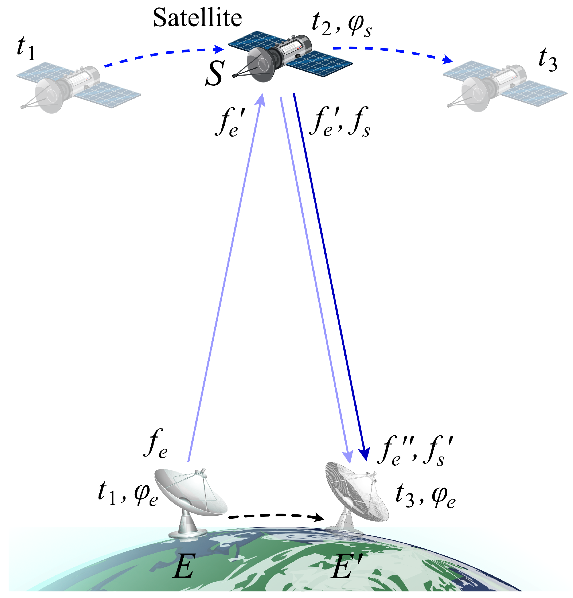
2.1. Gravity Frequency Shift
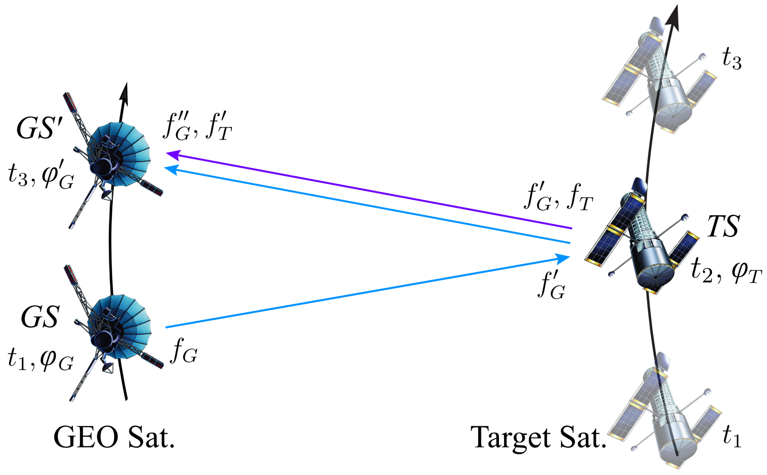
2.2. Determination of Gravitational Potential along the Target Satellite Orbit
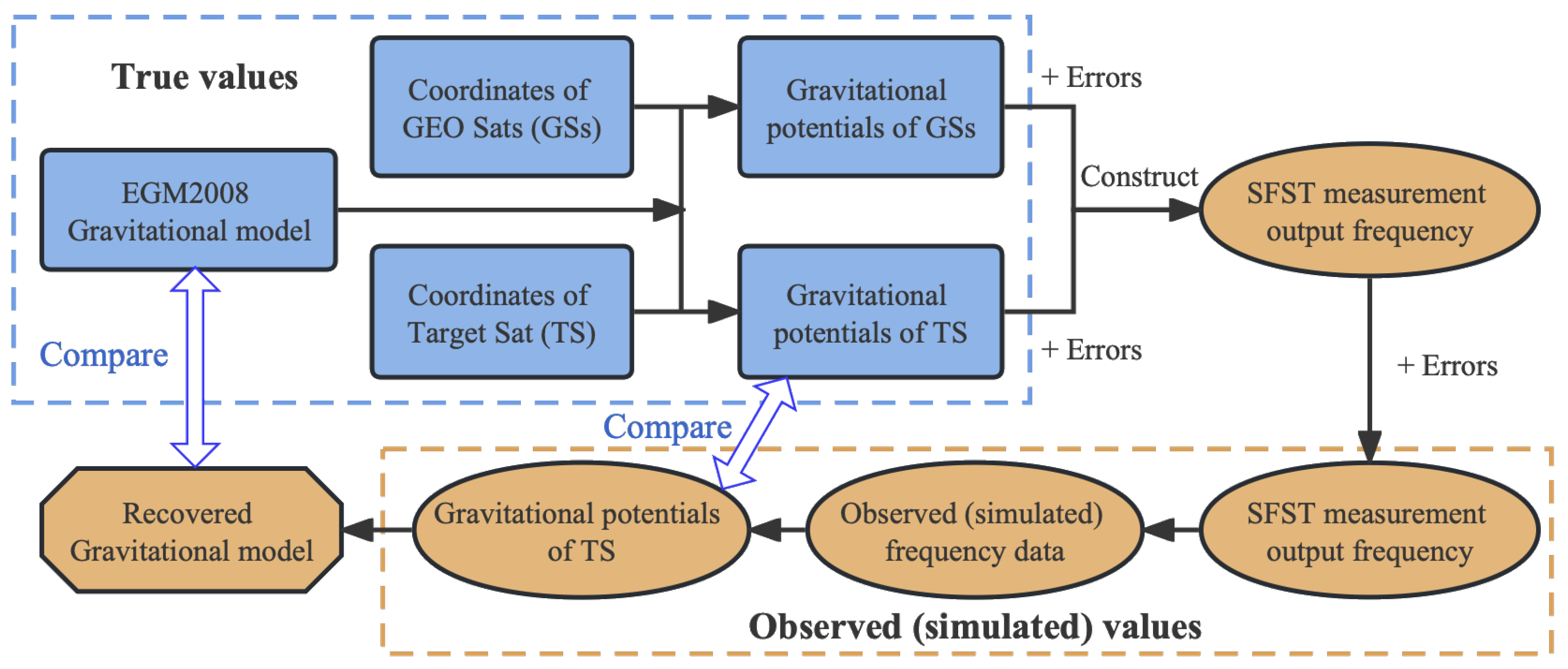
3. Simulation Experiments
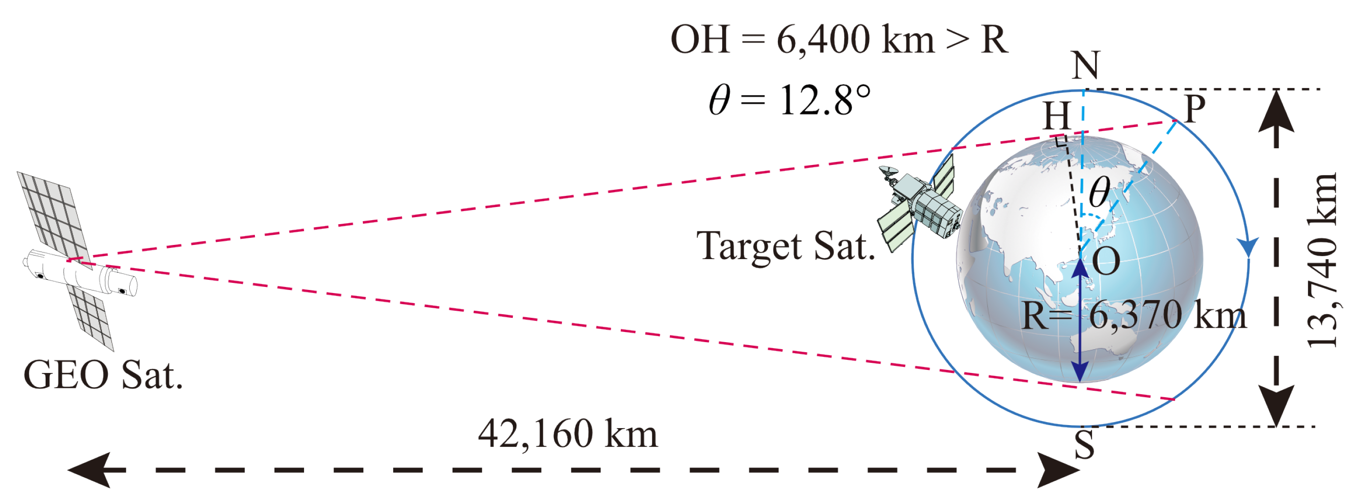
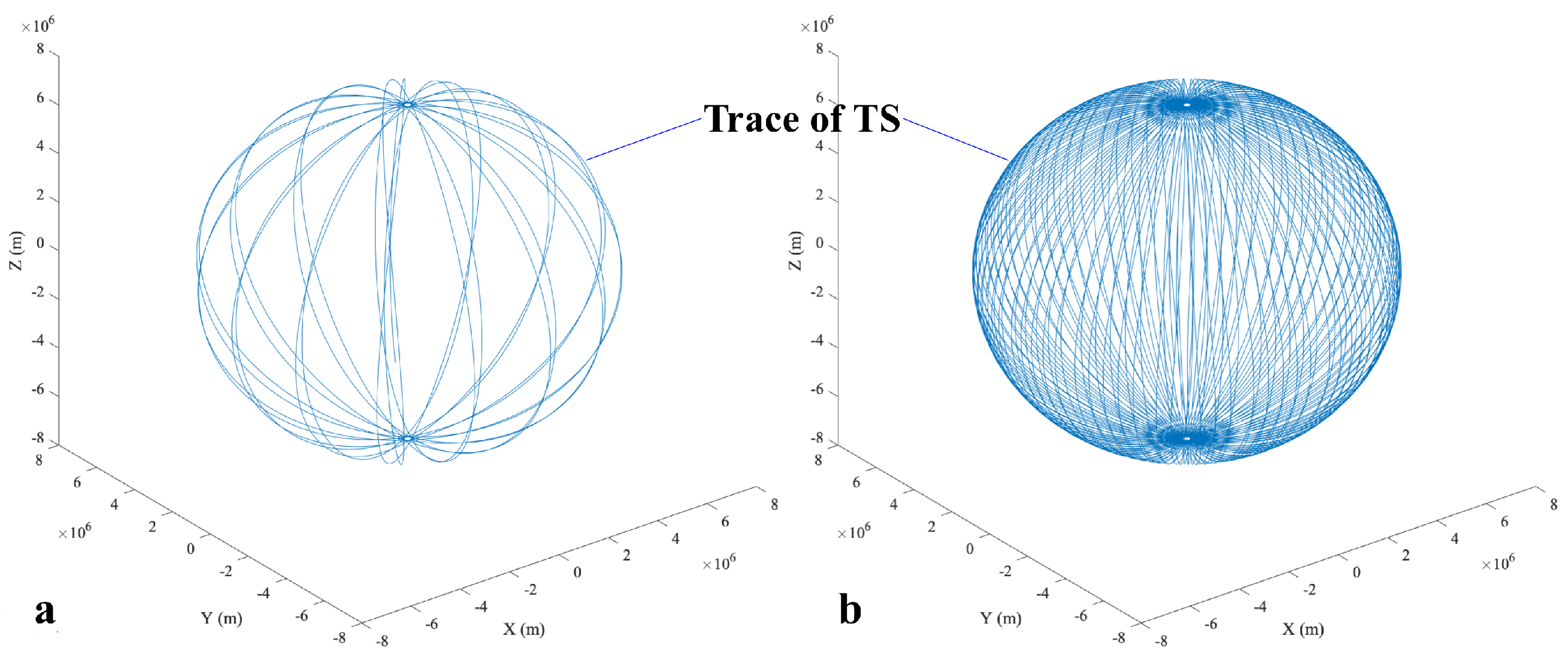
3.1. Input Data
3.2. The Simulated Observations of GP along the TS Orbit
3.3. Determining the Earth’s External Gravitational Field
4. Results
5. Conclusions
Author Contributions
Funding
Data Availability Statement
Acknowledgments
Conflicts of Interest
Abbreviations
| EGM | Earth Gravitational Model. |
| GEO | Geosynchronous Equatorial Orbit. |
| GNSS | Global Navigation Satellite Systems. |
| GOCE | Gravity Field and steady-state Ocean Circulation Explorer. |
| GP | Gravitational potential. |
| GRACE | Gravity Recovery and Climate Experiment. |
| GS | Geosynchronous Equatorial Orbit satellite. |
| IRI | International Reference Ionosphere. |
| LEO | Low-Earth Orbit. |
| OAC | Optical-atomic clock. |
| REGM | Recovered Earth Gravitational Model. |
| SD | Standard deviation. |
| SFST | Satellite frequency signal transfer. |
| TS | Target satellite. |
References
- Dziewonski, A.M.; Anderson, D.L. Preliminary reference Earth model. Phys. Earth Planet. Inter. 1981, 25, 297–356. [Google Scholar] [CrossRef]
- Hofmann-Wellenhof, B.; Moritz, H. Physical Geodesy; Springer: Berlin/Heidelberg, Germany, 2005; pp. 1–405. [Google Scholar]
- Kaula, W.M. Theory of Satellite Geodesy: Applications of Satellites to Geodesy; Dover Publications: Mineola, NY, USA, 1966. [Google Scholar]
- Reigber, C.; Schwintzer, P.; Lühr, H. The CHAMP geopotential mission. Boll. Geof. Teor. Appl. 1999, 40, 285–289. [Google Scholar]
- Tapley, B.D.; Bettadpur, S.; Watkins, M.; Reigber, C. The gravity recovery and climate experiment: Mission overview and early results. Geophys. Res. Lett. 2004, 31, L09607. [Google Scholar] [CrossRef] [Green Version]
- Drinkwater, M.R.; Haagmans, R.; Muzi, D.; Popescu, A.; Floberghagen, R.; Kern, M.; Fehringer, M. The GOCE gravity mission: ESA’s first core Earth explorer. In Proceedings of the 3rd International GOCE User Workshop, Frascati, Italy, 6–8 November 2006; pp. 6–8. [Google Scholar]
- Ditmar, P.; van Eck van der Sluijs, A.A. A technique for modeling the Earth’s gravity field on the basis of satellite accelerations. J. Geod. 2004, 78, 12–33. [Google Scholar] [CrossRef]
- Hwang, C. Gravity recovery using COSMIC GPS data: Application of orbital perturbation theory. J. Geod. 2001, 75, 117–136. [Google Scholar] [CrossRef] [Green Version]
- Reubelt, T.; Austen, G.; Grafarend, E.W. Harmonic analysis of the Earth’s gravitational field by means of semi-continuous ephemerides of a low Earth orbiting GPS-tracked satellite. Case study: CHAMP. J. Geod. 2003, 77, 257–278. [Google Scholar] [CrossRef]
- Jekeli, C. The determination of gravitational potential differences from satellite-to-satellite tracking. Celest. Mech. Dyn. Astron. 1999, 75, 85–101. [Google Scholar] [CrossRef]
- Han, S.C.; Jekeli, C.; Shum, C.K. Efficient gravity field recovery using in situ disturbing potential observables from CHAMP. Geophys. Res. Lett. 2002, 29, 36-1–36-4. [Google Scholar] [CrossRef] [Green Version]
- Visser, P.N.A.M.; Sneeuw, N.; Gerlach, C. Energy integral method for gravity field determination from satellite orbit coordinates. J. Geod. 2003, 77, 207–216. [Google Scholar] [CrossRef] [Green Version]
- Oelker, E.; Hutson, R.B.; Kennedy, C.J.; Sonderhouse, L.; Bothwell, T.; Goban, A.; Kedar, D.; Sanner, C.; Robinson, J.M.; Marti, G.E.; et al. Demonstration of 4.8 × 10⁻¹⁷ stability at 1 s for two independent optical clocks. Nat. Photonics 2019, 13, 714–719. [Google Scholar] [CrossRef] [Green Version]
- Nakamura, T.; Davila-Rodriguez, J.; Leopardi, H.; Sherman, J.A.; Fortier, T.M.; Xie, X.; Campbell, J.C.; McGrew, W.F.; Zhang, X.; Hassan, Y.S.; et al. Coherent optical clock down-conversion for microwave frequencies with 10–18 instability. Science 2020, 368, 889–892. [Google Scholar] [CrossRef] [PubMed]
- Zheng, X.; Dolde, J.; Lochab, V.; Merriman, B.N.; Li, H.; Kolkowitz, S. Differential clock comparisons with a multiplexed optical lattice clock. Nature 2022, 602, 425–430. [Google Scholar] [CrossRef] [PubMed]
- Hannig, S.; Pelzer, L.; Scharnhorst, N.; Kramer, J.; Stepanova, M.; Xu, Z.T.; Spethmann, N.; Leroux, I.D.; Mehlstäubler, T.E.; Schmidt, P.O. Towards a transportable aluminium ion quantum logic optical clock. Rev. Sci. Instrum. 2019, 90, 053204. [Google Scholar] [CrossRef] [Green Version]
- Jaduszliwer, B.; Camparo, J. Past, present and future of atomic clocks for GNSS. GPS Solut. 2021, 25, 27. [Google Scholar] [CrossRef]
- Einstein, A. Die Feldgleichungen der Gravitation. Sitzungsberichte Königlich Preuss. Akad. Wiss. 1915, 25, 844–847. [Google Scholar]
- Shen, W.; Ning, J.; Liu, J.; Li, J.; Chao, D. Determination of the geopotential and orthometric height based on frequency shift equation. Nat. Sci. 2011, 3, 388–396. [Google Scholar] [CrossRef] [Green Version]
- Shen, Z.; Shen, W.B.; Zhang, S. Formulation of geopotential difference determination using optical-atomic clocks onboard satellites and on ground based on Doppler cancellation system. Geophys. J. Int. 2016, 206, 1162–1168. [Google Scholar] [CrossRef] [Green Version]
- Shen, Z.; Shen, W.B.; Zhang, S. Determination of gravitational potential at ground using optical-atomic clocks on board satellites and on ground stations and relevant simulation experiments. Surv. Geophys. 2017, 38, 757–780. [Google Scholar] [CrossRef] [Green Version]
- Weinberg, S. Gravitation and Cosmology: Principles and Applications of the General Theory of Relativity; Wiley: New York, NY, USA, 1972. [Google Scholar]
- Bjerhammar, A. On a relativistic geodesy. Bull. Am. Assoc. Hist. Nurs. 1985, 59, 207–220. [Google Scholar] [CrossRef]
- Flury, J. Relativistic geodesy. J. Phys. Conf. Ser. 2016, 723, 012051. [Google Scholar] [CrossRef]
- Puetzfeld, D.; Lämmerzahl, C. (Eds.) Relativistic Geodesy: Foundations and Applications; Springer: Cham, Switzerland, 2019. [Google Scholar]
- Kopeikin, S.M.; Kanushin, V.F.; Karpik, A.P.; Tolstikov, A.S.; Gienko, E.G.; Goldobin, D.N.; Kosarev, N.S.; Ganagina, I.G.; Mazurova, E.M.; Karaush, A.A.; et al. Chronometric measurement of orthometric height differences by means of atomic clocks. Gravit. Cosmol. 2016, 22, 234–244. [Google Scholar] [CrossRef]
- Grotti, J.; Koller, S.; Vogt, S.; Häfner, S.; Sterr, U.; Lisdat, C.; Denker, H.; Voigt, C.; Timmen, L.; Rolland, A.; et al. Geodesy and metrology with a transportable optical clock. Nat. Phys. 2018, 14, 437–441. [Google Scholar] [CrossRef] [Green Version]
- Takano, T.; Takamoto, M.; Ushijima, I.; Ohmae, N.; Akatsuka, T.; Yamaguchi, A.; Kuroishi, Y.; Munekane, H.; Miyahara, B.; Katori, H. Geopotential measurements with synchronously linked optical lattice clocks. Nat. Photonics 2016, 10, 662. [Google Scholar] [CrossRef]
- Wu, H.; Müller, J.; Lämmerzahl, C. Clock networks for height system unification: A simulation study. Geophys. J. Int. 2019, 216, 1594–1607. [Google Scholar] [CrossRef]
- Shen, Z.; Shen, W.B.; Peng, Z.; Liu, T.; Zhang, S.; Chao, D. Formulation of determining the gravity potential difference Using ultra-high precise clocks via optical fiber frequency transfer technique. J. Earth Sci. 2019, 30, 422–428. [Google Scholar] [CrossRef]
- Deschênes, J.D.; Sinclair, L.C.; Giorgetta, F.R.; Swann, W.C.; Baumann, E.; Bergeron, H.; Cermak, M.; Coddington, I.; Newbury, N.R. Synchronization of distant optical clocks at the femtosecond Level. Phys. Rev. X 2016, 6, 021016. [Google Scholar] [CrossRef] [Green Version]
- Kleppner, D.; Vessot, R.F.C.; Ramsey, N.F. An orbiting clock experiment to determine the gravitational red shift. Astrophys. Space Sci. 1970, 6, 13–32. [Google Scholar] [CrossRef]
- Vessot, R.F.C.; Levine, M.W. A test of the equivalence principle using a space-borne clock. Gen. Relat. Grav. 1979, 10, 181–204. [Google Scholar] [CrossRef]
- Vessot, R.F.C.; Levine, M.W.; Mattison, E.M.; Blomberg, E.L.; Hoffman, T.E.; Nystrom, G.U.; Farrel, B.F.; Decher, R.; Eby, P.B.; Baugher, C.R.; et al. Test of relativistic gravitation with a space-borne hydrogen maser. Phys. Rev. Lett. 1980, 45, 2081–2084. [Google Scholar] [CrossRef]
- Müller, J.; Wu, H. Using quantum optical sensors for determining the Earth’s gravity field from space. J. Geod. 2020, 94, 71. [Google Scholar] [CrossRef]
- Shen, Z.; Shen, W.; Zhang, S. Determination of the gravitational potential at GOCE-type satellite orbit using frequency signal transmission approach. In Proceedings of the 20st EGU General Assembly, EGU2018, Vienna, Austria, 8–13 April 2018; p. 19415. [Google Scholar]
- Pierno, L.; Varasi, M. Switchable Delays Optical Fibre Transponder with Optical Generation of Doppler Shift. U.S. Patent 8,466,831, 18 June 2013. [Google Scholar]
- Heiskanen, W.A.; Moritz, H. Physical geodesy. Bull. Geod. 1967, 86, 491–492. [Google Scholar] [CrossRef]
- Liu, L.; Lü, D.S.; Chen, W.B.; Li, T.; Qu, Q.Z.; Wang, B.; Li, L.; Ren, W.; Dong, Z.R.; Zhao, J.B.; et al. In-orbit operation of an atomic clock based on laser-cooled 87Rb atoms. Nat. Commun. 2018, 9, 2760. [Google Scholar] [CrossRef] [PubMed] [Green Version]
- Pavlis, N.K.; Holmes, S.A.; Kenyon, S.C.; Factor, J.K. The development and evaluation of the Earth Gravitational Model 2008 (EGM2008). J. Geophys. Res. Solid Earth 2012, 117, B04406. [Google Scholar] [CrossRef] [Green Version]
- Croitoru, E.I.; Oancea, G. Satellite tracking using norad two-line element set format. AFASES 2016, 18, 423–432. [Google Scholar] [CrossRef]
- Bilitza, D.; Altadill, D.; Truhlik, V.; Shubin, V.; Galkin, I.; Reinisch, B.; Huang, X. International reference ionosphere 2016: From ionospheric climate to real-time weather predictions. Space Weather 2017, 15, 418–429. [Google Scholar] [CrossRef]
- Namazov, S.A.; Novikov, V.D.; Khmel’nitskii, I.A. Doppler frequency shift during ionospheric propagation of decameter radio waves. Radiophys. Quantum Electron. 1975, 18, 345–364. [Google Scholar] [CrossRef]
- Voigt, C.; Förste, C.; Wziontek, H.; Crossley, D.; Meurers, B.; Pálinkáš, V.; Hinderer, J.; Boy, J.P.; Barriot, J.P.; Sun, H. The Data Base of the International Geodynamics and Earth Tide Service (IGETS). In Proceedings of the 19th EGU General Assembly, EGU2017, Vienna, Austria, 23–28 April 2017; p. 4947. [Google Scholar]
- Van Camp, M.; Vauterin, P. Tsoft: Graphical and interactive software for the analysis of time series and Earth tides. Comput. Geosci. 2005, 31, 631–640. [Google Scholar] [CrossRef]
- Wenzel, H.G. The nanogal software: Earth tide data processing package ETERNA 3.30. Bull. Inf. Marées Terrestres 1996, 124, 9425–9439. [Google Scholar]
- Joernc. Tidal-Potential. 2018. Available online: https://github.com/joernc/tidal-potential (accessed on 10 March 2023).
- Major, F.G. The Quantum Beat: The Physical Principles of Atomic Clocks; Springer Science & Business Media: Berlin/Heidelberg, Germany, 2013. [Google Scholar]
- Galleani, L.; Sacerdote, L.; Tavella, P.; Zucca, C. A mathematical model for the atomic clock error. Metrologia 2003, 40, S257. [Google Scholar] [CrossRef]
- Sharifi, M.A.; Seif, M.R.; Hadi, M.A. A comparison between numerical differentiation and kalman filtering for a leo satellite velocity determination. Artif. Satell. 2013, 48, 103–110. [Google Scholar] [CrossRef] [Green Version]
- Li, X.; Zhu, Y.; Zheng, K.; Yuan, Y.; Liu, G.; Xiong, Y. Precise Orbit and Clock Products of Galileo, BDS and QZSS from MGEX Since 2018: Comparison and PPP Validation. Remote Sens. 2020, 12, 1415. [Google Scholar] [CrossRef]
- Shen, P.; Cheng, F.; Lu, X.; Xiao, X.; Ge, Y. An Investigation of Precise Orbit and Clock Products for BDS-3 from Different Analysis Centers. Sensors 2021, 21, 1596. [Google Scholar] [CrossRef] [PubMed]
- Davies, K.; Watts, J.M.; Zacharisen, D.H. A study of F 2 -layer effects as observed with a Doppler technique. J. Geophys. Res. 1962, 67, 601–609. [Google Scholar] [CrossRef]
- Hoque, M.M.; Jakowski, N. Higher order ionospheric effects in precise GNSS positioning. J. Geod. 2007, 81, 259–268. [Google Scholar] [CrossRef]
- Rama Rao, P.V.S.; Niranjan, K.; Prasad, D.; Gopi Krishna, S.; Uma, G. On the validity of the ionospheric pierce point (IPP) altitude of 350 km in the Indian equatorial and low-latitude sector. Ann. Geophys. 2006, 24, 2159–2168. [Google Scholar] [CrossRef] [Green Version]
- Harville, D. Extension of the Gauss-Markov theorem to include the estimation of random effects. Ann. Statist. 1976, 4, 384–395. [Google Scholar] [CrossRef]


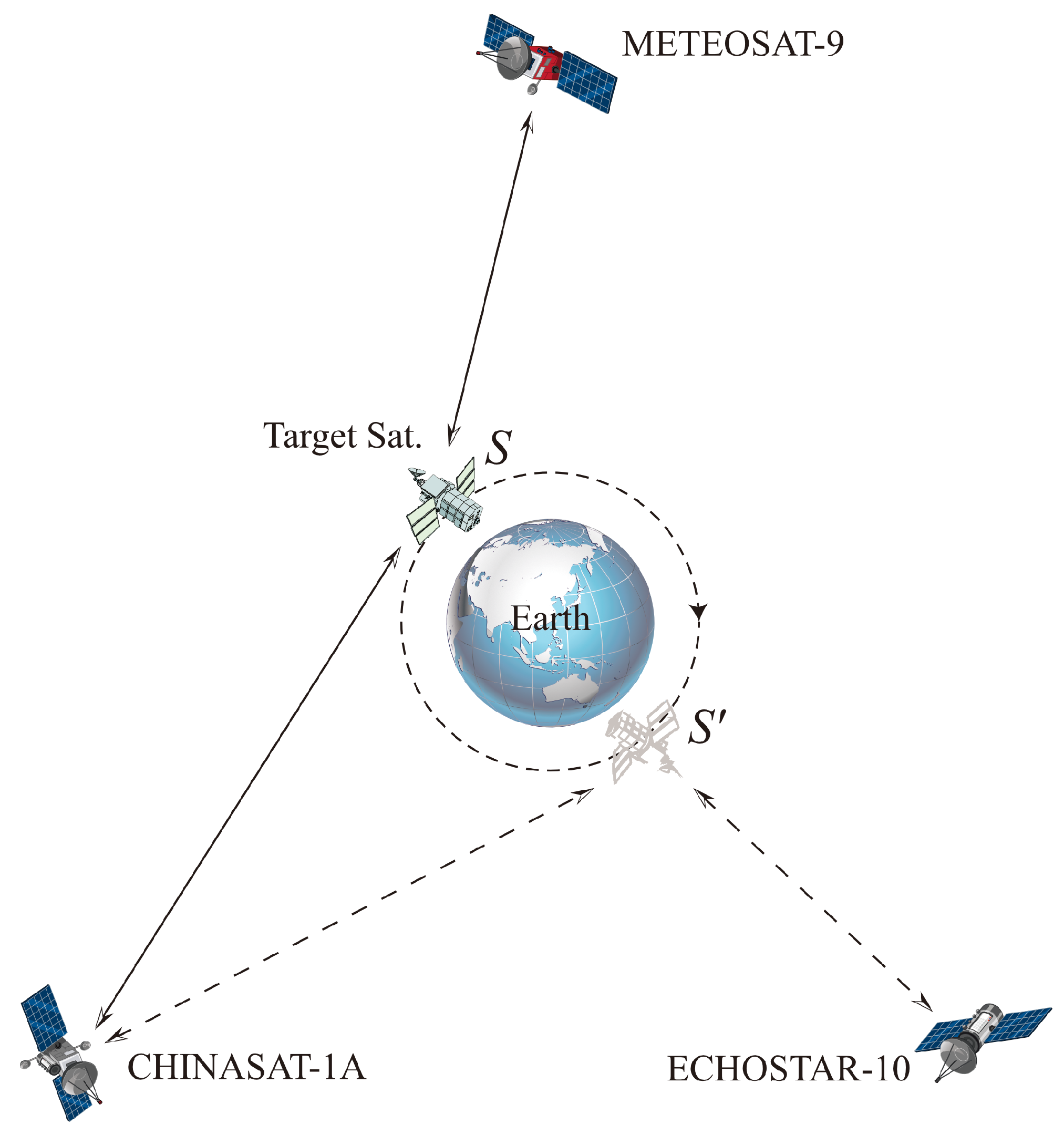
| Entities | Values of Parameters |
|---|---|
| GS Satellite | METEOSAT-9 ( GHz) |
| CHINASAT-1A ( GHz) | |
| ECHOSTAR-10 ( GHz) | |
| TS Satellite | GRACE-FO 1 |
| Gravity field model | EGM2008 |
| Ionospheric model | International Reference Ionosphere |
| Tide correction | Tidal Potential |
| Observation duration | 1∼30 January 2023 |
| Mearsurement interval | 1 s |
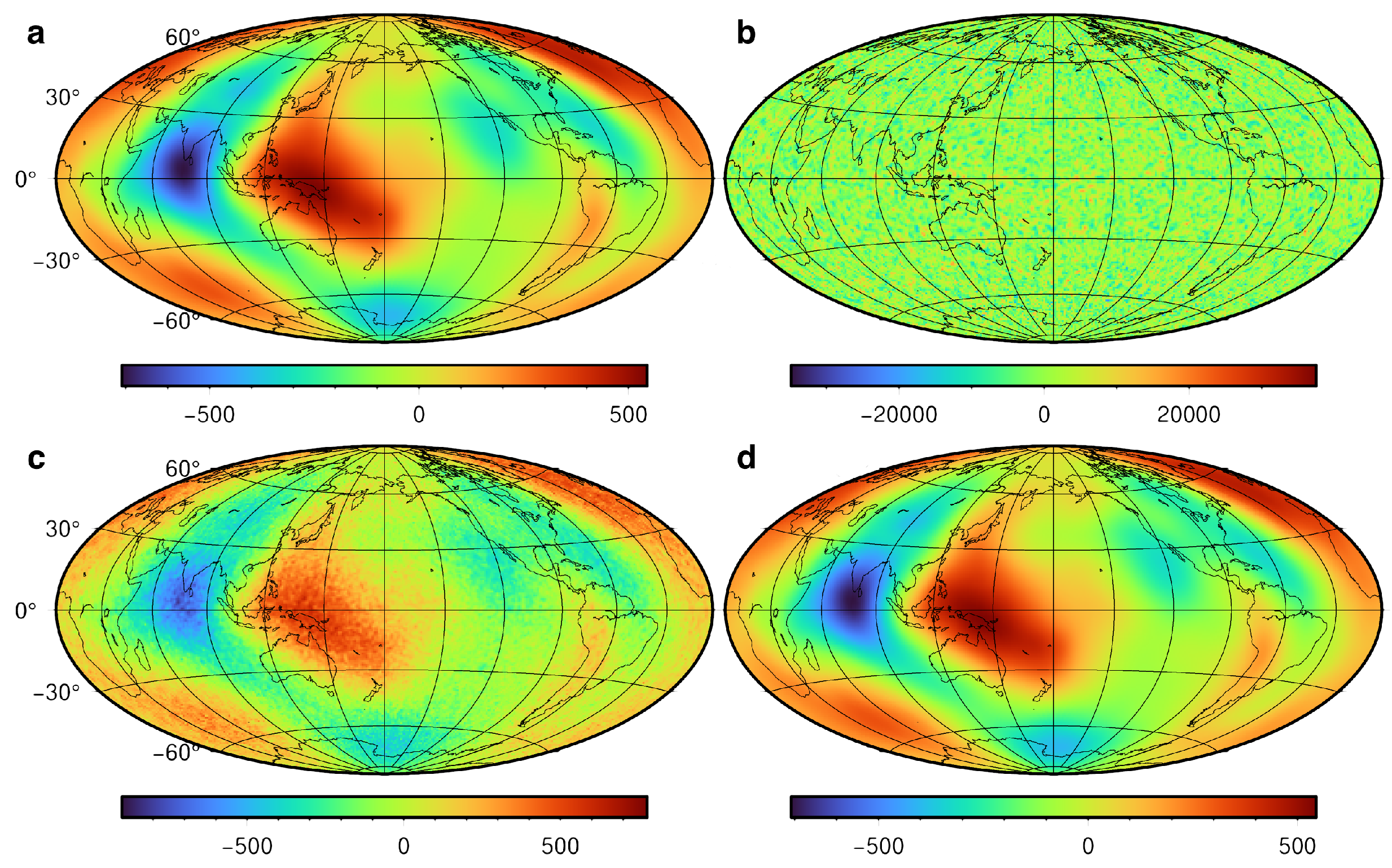
| Influence Factor | (Residual) Error Magnitude in |
|---|---|
| Ionospheric correction residual | |
| Tidal correction residual | |
| Position error | |
| Velocity error | |
| Gravitational potential error | |
| Clock error | , , |
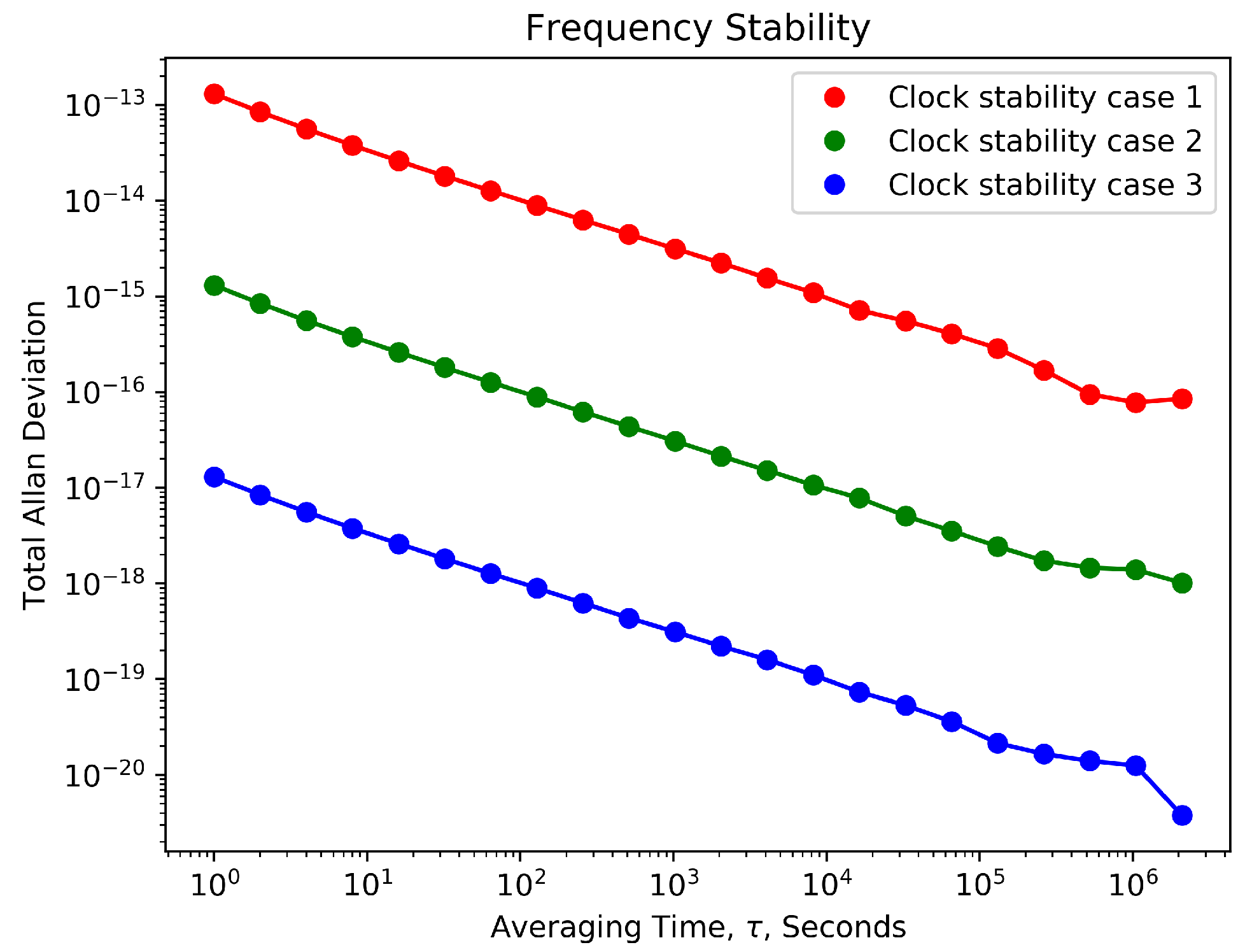
| Case | Clock Instability | Mean Offset () | Standard Deviation () |
|---|---|---|---|
| 1 | 1.200 | 12,815.256 | |
| 2 | 0.243 | 128.086 | |
| 3 | −1.86 × | 1.662 |
| Case | Clock Instability | Mean Offset () | Standard Deviation () |
|---|---|---|---|
| 1 | 1.063 | 1320.475 | |
| 2 | 0.243 | 13.231 | |
| 3 | −1.08 × | 0.143 | |
| 4 | −1.17 × | 0.014 | |
| 5 | −2.94 × | 1.47 × | |
| 6 | 0 | 2.74 × | 6.96 × |
Disclaimer/Publisher’s Note: The statements, opinions and data contained in all publications are solely those of the individual author(s) and contributor(s) and not of MDPI and/or the editor(s). MDPI and/or the editor(s) disclaim responsibility for any injury to people or property resulting from any ideas, methods, instructions or products referred to in the content. |
© 2023 by the authors. Licensee MDPI, Basel, Switzerland. This article is an open access article distributed under the terms and conditions of the Creative Commons Attribution (CC BY) license (https://creativecommons.org/licenses/by/4.0/).
Share and Cite
Shen, Z.; Shen, W.; Xu, X.; Zhang, S.; Zhang, T.; He, L.; Cai, Z.; Xiong, S.; Wang, L. A Method for Measuring Gravitational Potential of Satellite’s Orbit Using Frequency Signal Transfer Technique between Satellites. Remote Sens. 2023, 15, 3514. https://doi.org/10.3390/rs15143514
Shen Z, Shen W, Xu X, Zhang S, Zhang T, He L, Cai Z, Xiong S, Wang L. A Method for Measuring Gravitational Potential of Satellite’s Orbit Using Frequency Signal Transfer Technique between Satellites. Remote Sensing. 2023; 15(14):3514. https://doi.org/10.3390/rs15143514
Chicago/Turabian StyleShen, Ziyu, Wenbin Shen, Xinyu Xu, Shuangxi Zhang, Tengxu Zhang, Lin He, Zhan Cai, Si Xiong, and Lingxuan Wang. 2023. "A Method for Measuring Gravitational Potential of Satellite’s Orbit Using Frequency Signal Transfer Technique between Satellites" Remote Sensing 15, no. 14: 3514. https://doi.org/10.3390/rs15143514