Article

DASANet: A 3D Object Detector with Density-and-Sparsity Feature Aggregation

1
Remote Sensing Image Processing and Fusion Group, School of Electronic Engineering, Xidian University, Xi’an 710071, China
2
Hangzhou Institute of Technology, Xidian University, Hangzhou 311200, China
*
Author to whom correspondence should be addressed.
Remote Sens. 2023, 15(18), 4587; https://doi.org/10.3390/rs15184587
Submission received: 31 July 2023 / Revised: 13 September 2023 / Accepted: 14 September 2023 / Published: 18 September 2023

Abstract

:
In the field of autonomous driving and robotics, 3D object detection is a difficult, but important task. To improve the accuracy of detection, LiDAR, which collects the 3D point cloud of a scene, is updated constantly. But the density of the collected 3D points is low, and its distribution is unbalanced in the scene, which influences the accuracy of 3D object detectors in regards to object location and identification. Although corresponding high-resolution scene images from cameras can be used as supplemental information, poor fusion strategies can result in decreased accuracy compared with that of LiDAR-point-only detectors. Thus, to improve the detection performance for the classification, localization, and even boundary location of 3D objects, a two-stage detector with density-and-sparsity feature aggregation, called DASANet, is proposed in this paper. In the first stage, dense pseudo point clouds are generated with images from cameras and are used to obtain the initial proposals. In the second stage, two novel feature aggregation modules are designed to fuse LiDAR point information and pseudo point information, which refines the semantic and detailed representation of the feature maps. To supplement the semantic information of the highest-scale LiDAR features for object localization and classification, a triple differential information supplement (TDIS) module is presented to extract the LiDAR-pseudo differential features and enhance them in spatial, channel, and global dimensions. To increase the detailed information of the LiDAR features for object boundary location, a Siamese three-dimension coordinate attention (STCA) module is presented to extract stable LiDAR and pseudo point cloud features with a Siamese encoder and fuse these features using a three-dimension coordinate attention. Experiments using the KITTI Vision Benchmark Suite demonstrate the improved performance of our DASANet in regards to the localization and boundary location of objects. The ablation studies demonstrate the effectiveness of the TDIS and the STCA modules.

Graphical Abstract

1. Introduction

The subject of 3D object detection is a hot research topic in computer vision, which plays a significant role in autonomous driving, robot navigation, virtual reality, etc. Its primary objective is to determine an object’s location, identify its category, and provide the object’s range and orientation in 3D space. Cameras and LiDARs are commonly used sensors for 3D object detection. Cameras collect high-resolution RGB images of scenes, but these images lack depth information, while LiDARs collect point clouds that include depth information, but this information is sparse and unevenly distributed. Based on these two kinds of data, many 3D object detectors have been designed in recent years.
The detectors based on cameras include 2D-regression-based detectors [1,2,3,4,5,6,7] and pseudo-point-based detectors [8,9,10]. The pseudo-point-based detectors need to estimate the depth for RGB images and generate pseudo point clouds. Then 3D objects are detected with these point clouds. Although pseudo-point-based detectors need only images from cameras to generate dense points, the pseudo point clouds are not stable, which influences their 3D detection accuracy.
At the same time, numerous 3D detectors based on LiDAR have been proposed. With the different representations of point clouds, there are three types of detectors, i.e., voxel-based detectors [11,12,13,14,15,16,17,18], point-based detectors [19,20,21,22], and voxel-point-based detectors [23,24,25]. The voxel-based detectors partition the point clouds into distinct voxel grids and employ a 3D convolutional network to extract features, then perform detection using the voxel features. The point-based detectors use point-cloud networks [26,27,28] to directly extract features from point clouds and perform detection. The voxel-point-based detectors fuse voxel features and point features to perform detection. Although point clouds from LiDAR have better stability, these detectors are unable to obtain sufficient information in scenes using only their sparse point clouds, decreasing their object detection accuracy. We use 3D point clouds in the KITTI dataset as an example, and these are collected using a 64-beam Velodyne LiDAR. Figure 1 shows the histogram of these point clouds, including the number of object points and the corresponding detection accuracies at different distances. It can be seen that in a distance of more than 30 m, the LiDAR point number of an object is so small that it is difficult for the state-of-the-art LiDAR-point detector Voxel-RCNN to accurately detect the object. However, the corresponding image information can be considered as a beneficial supplement.
The detectors based on both LiDAR point clouds and their images have been researched widely. The image-region-proposal detectors [29,30,31,32] and multi-view detectors [33,34,35,36] use images of scenes directly in the detection process. The former restricts detection regions in point clouds through images, and the latter utilizes image features and view features of point clouds to generate 3D bounding boxes. These detectors use only the 2D space information of images and image features from a 2D convolutional neural network [37], and their performance is not satisfactory. Thus, the image information is explored further, especially the 3D space information from images, which is used to enrich LiDAR point information [38,39,40,41,42]. Figure 1 shows the 3D detection performance of our DASANet based on this strategy, which is noticeably better than that of the LiDAR-point detector.
In this work, the pixel depths in the images are estimated to generate pseudo point clouds of the scenes, and we design two aggregation modules to improve the semantic and boundary description ability of the LiDAR point features for objects. Based on these aggregation modules, i.e., the triple differential information supplement (TDIS) module and the Siamese three-dimension coordinate attention (STCA) module, we propose a novel two-stage 3D detector called DASANet. In the first stage, a LiDAR point cloud and its pseudo point cloud are used to generate initial proposals for the two modules of the second stage. In the TDIS module, to improve the classification and localization of objects, the difference between high-scale LiDAR features and their corresponding pseudo features is computed to obtain differential features with semantic information, and then the LiDAR features are supplemented with the stable differential features in spatial, channel, and global dimensions. To improve the boundary location of the objects, in the STCA module, a Siamese encoder is used to extract the LiDAR features and the stable pseudo point features; then, for detailed information enhancement, a three-dimension coordinate attention fuses the two kinds of features along the channel dimension, capturing their long-range dependencies [43] in 3D space. The final detection inference is based on the outputs of these modules.
In summary, our paper makes the following key contributions:
  • The novel triple differential information supplement (TDIS) module is designed to improve the feature description ability of object location and identification. In this module, the subtraction operation and three feature enhancement operations are used to obtain stable pseudo semantic features, which can supplement the LiDAR high-scale features with semantic information.
  • The novel Siamese three-dimension coordinate attention (STCA) module is designed to improve the boundary location of the 3D bounding box. In this module, a Siamese sparse encoder is used to extract the stable features from LiDAR and pseudo point clouds. Then, the three-dimension coordinate attention is designed to fuse each LiDAR feature and its corresponding pseudo point feature, according to their 3D space coordinates.
  • We conducted comprehensive experiments using a KITTI dataset to evaluate the performance of our DASANet. The results show that our network achieves significant improvement; specifically, for the objects with less than 100 points, the improvement is up to 15.59% in AP3D40.

2. Related Works

2.1. LiDAR-Based 3D Detector

For the data from LiDAR, there are three types of detectors for detecting a 3D object: voxel-based detectors, point-based detectors, and point-voxel detectors.
The voxel-based detectors convert point clouds into regular 3D or 2D layouts and achieve 3D detection using a network frame of 2D detectors. VoxelNet [11] partitions the space into 3D grids, groups the non-empty voxel points, and encodes the point features as voxel features. Subsequently, convolutional networks are utilized to extract features and predict the bounding boxes. SECOND [12] introduces sparse convolution [44,45] instead of conventional convolution in VoxelNet to accelerate its computational speed. PointPillars [13] divides the 3D space into pillars, encodes point features as non-empty pillar features, assembles them into pseudo images, and then employs 2D convolutional networks for high-speed detection. SA-SSD [14] adds precise point-level task auxiliary networks to assist the backbone network for 3D detection. Voxel-RCNN [16] uses SECOND as the RPN and designs voxel pooling to aggregate one-stage features and refine RPN predicted boxes to improve detection accuracy. Pyramid-RCNN [17] designs a pyramid-ROI to improve the features for the second stage. VoTr [18] uses sparse transformers instead of sparse convolutions to construct feature extraction networks.
The point-based detectors directly input the point cloud into the point feature extraction network and predict the bounding boxes for each point. VoteNet [21] uses PointNet++ [27] to extract the features and predicts the bounding boxes using surface point voting. PointRCNN [19] uses PointNet++ to construct a network for prediction point segmentation and foreground point box prediction. PointGNN [20] transforms the point cloud into a graph and inputs it into a graph convolutional neural network for feature extraction. CenterPoint [22] extends CenterNet [46] to the 3D space to achieve anchor-free 3D object detection based on key point prediction.
The point-voxel detectors combine voxels and points to improve the detection performance. STD [23] uses point networks in the first stage and encodes features into voxel features in the second stage to refine bounding box prediction. PV-RCNN [24] and PV-RCNN++ [25] use voxel networks in the first stage and add point features for prediction in the second stage.
Due to the sparsity and unbalance distribution of the point clouds, the detectors based on LiDAR do not perform well in regards to long-distance and occluded objects. In the corresponding images, objects have a large number of pixels, which can be used to improve the detection performance.

2.2. LiDAR-Camera-Based 3D Detector

LiDAR-camera-based 3D detectors, which include image-region-proposal detectors, multi-view detectors, and LiDAR-pseudo-point detectors, use images as an additional information resource to detect 3D objects.
The image-region-proposal detectors restrict 3D object detection within the back-projection areas of the proposal regions in the images. F-PointNet [29] leverages 2D detectors to drive 3D detection. It employs PointNet to estimate the frustum area associated with each 2D detection box and uses it to predict the corresponding 3D bounding box. PointPainting [32] utilizes a 2D segmentation network to acquire RGB foreground data and incorporates relevant semantic information into the point clouds to enhance the accuracy of 3D detection.
The multi-view detectors use multiple views of a point cloud and its corresponding images as input data for object detection. AVOD [33] inputs RGB images and BEV features into the FPN [47] to obtain full resolution feature maps. After data level fusion and ROI level fusion, class labels and 3D-box regression parameters are obtained. MV3D [34] first generates 3D ROIs using RPN on the BEV and then deeply fuses the BEV features, LiDAR front-facing features, and image features to obtain the regression results. CLOCs [35] use the geometric and semantic consistency of objects to promote each other and to reduce the occurrence of both false and missed detection. FusionRCNN [36] designs a second-stage transformer mechanism to achieve fusion between image features and 3D point features.
The LiDAR-pseudo-point detectors project images into 3D space to supplement the LiDAR point cloud for 3D object detection. MVP [39] unprojects image points near projections of the 3D points in the range of a 2D box to generate pseudo points. Focals Conv [40] introduces focal sparse convolution, which uses positional importance to obtain accurate features and improve 3D detection performance. VFF [41] maintains cross-modal consistency with enhanced image-feature-rays in the voxel field and uses the ray-wise fusion for 3D detection. SFD [42] uses deep completion networks [48,49] to obtain dense pseudo points, and in the second stage, improves the results of 3D object detection by neighbor searching in images and 3D grid attention in 3D space.
Compared with image-region-proposal and multi-view detectors, the LiDAR-pseudo-point detectors utilize image information and LiDAR point information more deeply and achieve better detection results, which also alleviates image information perturbations in camera-only detectors [50]. We adopt the concept of LiDAR-pseudo-point detectors to propose a novel 3D detection network.

3. Methodology

Using the pseudo point clouds, which inherit the information from RGB images to densify the space information, two aggregation modules are designed in our 3D object detector, DASANet. The triple differential information supplement (TDIS) module is used to improve the object location and identification ability. The Siamese three-dimension coordinate attention (STCA) module is used to improve the object boundary location ability. In this section, we will present our DASANet in detail, specifically the two feature aggregation modules.

3.1. Architecture

The architecture overview of our DASANet is shown in Figure 2. In this network, depth completion [48] is first used with the LiDAR point clouds and their corresponding images to generate dense point clouds in the LiDAR coordinate system [51,52], which include pseudo points. Then, two sparse convolution networks with different weights extract the LiDAR 3D feature maps and the pseudo 3D feature maps, with the regular voxels divided from the LiDAR point clouds and pseudo point cloud [11], respectively. With the concatenated feature maps from their highest-scale feature maps, a region proposal network (RPN) [53] is used to generate initial 3D proposals, i.e., ROIs. To enhance the semantic information load of the features in each ROI for further determination of their class label and location, the two highest-scale feature maps from each sparse convolution networks are interpolated onto the grids of the ROIs, based on the Manhattan distance [16], and the new ROI features are input into the proposed TDIS module to generate semantic-supplemented features. Meanwhile, to enhance the boundary localization ability of the features, the ROI LiDAR points and the ROI pseudo points cropped from the two kinds of point clouds [19,24] are input into the designed STCA module to generate local-refined features. Finally, with their concatenated feature maps, the initial proposals are further refined to generate the bounding box predictions using the detection head, which comprises one shared MLP and two output MLPs for classification and regression.

3.2. TDIS Module

In 3D object location, LiDAR point clouds play an important role. This is because the point clouds collected by an active sensor exhibit good stability and can reflect, to a certain degree, the structural information of 3D objects. However, LiDAR points are produced by the reflection of laser beams, which have a fixed angular resolution, and the density of the laser beams decreases with the increase in distance and the enlargement of the view field; thus, the point clouds show a sparse and even unbalanced distribution, which leads to unsatisfactory detection results. In our network, their corresponding RGB images, which possess a uniform information load distribution to describe each captured object, are used to produce dense pseudo points. For the LiDAR point clouds, their pseudo point clouds can supplement structural information, whose feature maps can then be used to improve the classification and location performance. But their estimated space depths lack stability; thus, we select their two highest-scale feature maps, which are comparatively stable, to generate the inputs of our TDIS module. With the interpolation operation, a linear mapping and the channel dimension concatenation operation [16], the flattened ROI feature maps of the LiDAR points and pseudo points are obtained and are first input into a subtraction operation in the TDIS module. The subtraction operation can remove the redundant information from the LiDAR features in the ROI features of the pseudo points to generate differential features. Then, for the differential features, three feature enhancement operations—spatial dimension, channel dimension, and global dimensions—are used to generate more stable semantic feature maps. Finally, the spatial feature maps, the channel feature maps, and the global features supplement the ROI features of the LiDAR points to produce semantic-supplemented feature maps. The architecture of the TDIS module is shown in Figure 3.
With the LiDAR ROI feature map F S and the pseudo ROI feature map F P , which are obtained by flattening the 3D features of each channel in the original 3D feature map into a one-dimensional vector, as inputs, the differential feature map F D is computed using element subtraction. The calculation process of each element is described by Equation (1).
F D i , j = F P i , j F S i , j
where F D i , j , F P i , j , and F S i , j denote the feature at the channel i and in the location j of the feature map F D , F P , and F S , which all have C channels and N locations.
Then, the feature map F D is used to obtain three stable semantic feature maps by three feature enhancement operations in the spatial dimension, channel dimension, and global dimensions, which are followed by corresponding feature supplementation operations. To enhance the feature map in the spatial dimension, the F D is weighted by all N learnable spatial weight matrices W l S p in W S p , and then all the elements in each weighted feature map are added up as Equation (2).
F S p l = i = 1 C j = 1 N W l S p i , j F D i , j l = 1 , 2 , , N
where all F S p l can be used to compose a one-dimensional raw vector F S p l , i.e., the spatial feature map F S p . To obtain the spatial-supplemented feature map F S p T , each element of F S p is added to the corresponding element of F S on all the C channels, which can be described by Equation (3).
F S p T = F S + A C h F S p
where A C h is a C -dimension column vector whose elements are all ones.
To enhance the feature map in the channel dimension, the F D is weighted by all C -learnable channel weight matrices W k C h in W C h , and then all the elements in each weighted feature map are added up as Equation (4).
F C h k = i = 1 C j = 1 N W k C h i , j F D i , j k = 1 , 2 , , C
where all F C h k can be used to compose a one-dimensional column vector F C h k , i.e., the channel feature map F C h . To obtain the spatial-channel-supplemented feature map F S p C h T , F C h is added to F S p T along the channels at their all spatial locations, which can be described by Equation (5).
F S p C h T = F S p T + F C h A S p
where A S p is an N -dimension row vector whose elements are all ones.
To enhance the feature map in global dimensions, the F D is weighted by a learnable global weight matrix W G o , and then these are added to obtain the global feature F G o as Equation (6).
F G o = i = 1 C j = 1 N W G o ( i , j ) F D ( i , j )
To obtain the semantic-supplemented feature map F T , F G o is added to each element of F S p C h T , which can be described by Equation (7).
F T = F S p C h T + F G o A
where A is an all-one matrix with the same size of F S .
In the TDIS module, the three semantic feature maps are computed using the same operation, but the spatial feature enhancement operation adds the same feature values to the corresponding spatial locations for all channels of F S , the channel feature enhancement operation adds the same feature values to the corresponding channels for all spatial locations of F S , and the global feature enhancement operation adds one feature value to each element of F S . Thus, during training, W S p , W C h , and W G o are optimized with spatial information, channel information, and global information, respectively.

3.3. STCA Module

Compared with the high-scale features, which contain semantic information for classification and location, the low-scale features contain detailed information, such as the edges and surfaces of objects, and even the shapes of their local structures [54]. In object detection tasks, most networks [16,17,19] use only high-scale features to obtain the classification and regression of bounding boxes results, which leads to inaccurate object ranges and boundaries. To improve the boundary localization ability, we design the Siamese three-dimension coordinate attention (STCA) module, which takes the LiDAR points and the pseudo points cropped from the ROIs as inputs to obtain the elaborate low-scale features. In this module, the Siamese sparse encoder, which has two identical architecture networks with shared weights, extracts the features from two ROI point clouds at the same time. Because the features of the two feature maps extracted by the Siamese encoder are similar, the features from the sparse LiDAR points that are not easy to change will affect the features from the pseudo points, improving its stability. With the channel concatenation of the two feature maps, the three-dimension coordinate attention (TCA) is designed to fuse these feature maps along the channel dimension, capturing the long-range dependencies along each of three spatial directions. For example, the TCA highlights the channels of the input feature maps and outputs position-sensitive attention feature maps.
Figure 4 shows the architecture of the STCA module, which consists of the Siamese sparse encoder and the three-dimension coordinate attention. In the Siamese sparse encoder, with the LiDAR point cloud P S and the pseudo point cloud P P cropped in an ROI as inputs, a weight-shared two-layer MLP is used to preliminarily extract two groups of point features. Then, these point features are divided into two groups of voxel grids, with adaptive size based on ROIs, to obtain 3D grid features [11]. Finally, the 3D grid features are fed into a weight-shared sparse convolution network with two submanifold convolution layers and one villain sparse convolution layer to generate the output feature maps F E S and F E P , corresponding to P S and P P [44,45].
With the channel concatenation of F E S and F E P , the concatenated feature map F C is input into the TCA, as shown in Figure 5. In the squeeze step, three spatial coordinates in the spatial dimension, which correspond to the x direction, the y direction, and the z direction, are taken into account. Thus, the global average pooling is expanded to 3D feature maps and implemented to the feature planes along each spatial coordinate, and the pooling outputs of the channel c in the channel dimension at length x , width y , and height z can be formulated as
α X x , c = 1 W × H k = 1 H j = 1 W F c C x , j , k
α Y y , c = 1 L × H k = 1 H i = 1 L F c C i , y , k
α Z z , c = 1 L × W j = 1 W i = 1 L F c C i , j , z
where L , W , and H denote the length, width, and height of F C , respectively, and F c C denotes the feature map of the channel c in F C .
To generate attention weights g X , g Y , and g Z in three spatial coordinates, 1 × 1 convolution operations are first implemented to the aggregated feature maps. But, for objects on the road, their distributions are parallel with the surface of the road, which means that objects in the x direction and the y direction have similar distribution properties for object detection, and their distributions in the height z direction are specific by contrast. Thus, the same convolutional transformation function C o n v X Y is used in both the x direction and the y direction, while another convolutional transformation function C o n v Z is used in the z direction. Then, three different 1 × 1 convolutional transformation functions, C o n v X g , C o n v Y g , and C o n v Z g , are used to separately transform the intermediate feature maps. This process can be formulated as
g X = σ C o n v X g δ C o n v X Y α X
g Y = σ C o n v Y g δ C o n v X Y α Y
g Z = σ C o n v Z g δ C o n v Z α Z
where C o n v X Y and C o n v Z output a feature map with 1/16 the number of channels of the input feature map; C o n v X g , C o n v Y g , and C o n v Z g output a feature map with the same number of channels as F C ; δ denotes the ReLU activation function; and σ denotes the sigmoid function.
Finally, the local-refined feature map F A is computed with the attention weights corresponding to three spatial coordinates, obtaining more accurate long-range dependence information in the spatial dimension. This process can be formulated as
F A i , j , k , c = F C i , j , k , c + F C i , j , k , c × g X i , c × g Y j , c × g Z k , c

3.4. Network Training

3.4.1. Auxiliary Head

During the training, two identical auxiliary heads are designed to be attached at the end of the TDIS module and the STCA module, in parallel with the detection head, improving the optimization direction and further accelerating the network convergence [14,42]. As shown in Figure 6, the auxiliary head consists of three two-layer MLPs, whose structure is same as the detection head, and the first MLP network takes the vector flattened from F T and F A . The other two MLPs are parallel, which predict the class labels and regression parameters of the bounding boxes for training.
Different from the detection head, which is input with the concatenated feature maps of the TDIS module and the STCA module, the auxiliary heads are attached to the two modules directly. Thus, during the training, when the back propagation from the detection head optimizes the TDIS module and the STCA module in balance, the auxiliary heads, which provide a specific effect on the corresponding module, provide individual optimization branches to the two modules in the optimization process, which improves the optimization ability of our network. During testing, the auxiliary heads are removed, without computational load, for network inference.

3.4.2. Loss Function

Our network DASANet is trained with a two-stage loss function, which consists of the RPN loss function L RPN for the first stage, and the RCNN loss function L RCNN for the second stage. The overall loss function L can be described by Equation (15).
L = L RPN + L RCNN
where L RPN is used to optimize the classification scores and the regression parameters of the RPN predicted boxes, which improves the detection performance of the ROIs [16]. L RCNN consists of three loss function, i.e., a detection head loss L det and two identical auxiliary head losses L a u x 1 and L a u x 2 , which are represented by Equation (16).
L RCNN = L det + λ 1 L a u x 1 + λ 2 L a u x 2
where λ 1 and λ 2 are the weights of L a u x 1 and L a u x 2 . L det optimizes the output of the detection head to improve the detection performance of the final predicted boxes. L a u x 1 and L a u x 2 optimize the outputs of the two auxiliary heads mentioned in Section 3.4.1 to upgrade the optimization ability and convergence speed of the network. L det , L a u x 1 , and L a u x 2 all consist of a classification loss and a regression loss. The classification loss is the binary cross-entropy loss [55]. In L det , the regression loss is the sum of the smooth L1 loss and the GIOU loss [56], which optimizes the IOU of the predicted boxes for the detection head and their eight vertexes. In L a u x 1 and L a u x 2 , the regression loss is simply the smooth L1 loss, which optimizes the encoded predicted boxes for the auxiliary head.

4. Experiments

In this section, we first introduce the dataset, metrics, and implementation details of our DASANet. Then, 3D detection and BEV detection experiments are used to evaluate the DASANet compared with fourteen state-of-the-art networks, and ablation experiments are conducted to verify the effectiveness of the TDIS and STCA modules in our network.

4.1. Datast and Evaluation Metrics

4.1.1. Dataset

The KITTI dataset [51,52] is a wide used autonomous driving dataset. The KITTI 3D/BEV object detection benchmark of this dataset, which contains 3D point cloud and RGB image data, is used in our experiments. The KITTI dataset consists of 7481 samples for training and 7518 samples for testing; in each sample, we use one 3D point cloud and a 1242 × 375 RGB image, collected by a 64-beam Velodyne LiDAR and a color camera with a resolution of 1392 × 512. For cars, as the compared category in our experiments, in all 3D-point-cloud scenes for training, there are 14,357 3D bounding boxes used as labels, and in each image for training, up to 15 cars are visible. For evaluation, we divide the training samples into a training split, with 3712 samples, and a validation split, with 3769 samples [51].

4.1.2. Metrics

We conduct experiments using the car as our category, an object which provides the most labels in the KITTI dataset. Every bounding box is classified into one of three difficulty levels: easy, moderate, and hard. These levels are defined based on their bounding box heights, their occlusion levels, and their truncation levels. An object with a bounding box height of more than 40 pixels, is fully visible, and shows less than 15% truncation is classified into the easy level. An object with a bounding box height of more than 25 pixels, is partly occluded, and exhibits less than 30% truncation is classified into the moderate level. An object with a bounding box height of more than 25 pixels, is difficult to see, and shows less than 50% truncation is classified into the hard level. We modify the average precision (AP) with an IOU threshold of 0.7 to evaluate the compared networks on the validation split. AP with N recall positions is calculated as Equation (17).
AP = i = 1 N Precision ( i ) N
where N denotes the number of the recall sample positions in the Precision-Recall curve, Precision ( i ) denotes the precision at the recall sample position i , which is determined by the class confidence threshold, and Precision = T P / T P + F P , TP denotes true positive prediction, and FP denotes false positive prediction. In the 3D detection experiments, AP3D11 and AP3D40 are calculated using 11 and 40 recall positions for the validation split. And, in the BEV detection experiments, the corresponding APBEV11 and APBEV40 are calculated using 11 and 40 recall positions. The KITTI dataset provides the labels of the training samples for training and validation, but the testing result is obtained by uploading the detection results on a testing split to the KITTI online server, which is calculated by the official metrics [52].

4.2. Implementation Details

In our network, TWISE [48] is used to generate depth maps with their official weights. After the depth maps are converted using transformation matrices [51,52] to generate pseudo point clouds in the LiDAR coordinate system, we set the range of each point cloud from 0 to 70.4 m along the x-direction, from −40 m to 40 m along the y direction, and from −3 m to 1 m along the z direction, then divide the LiDAR point clouds and pseudo point clouds into [0.05 m, 0.05 m, 0.1 m] voxels The maximum number of divided voxels is 16,000 during training and 40,000 during evaluation, which guarantees that each voxel contains up to 5 LiDAR points and 15 pseudo points. In our network, we set each anchor size at [1.6 m, 3.9 m 1.46 m] and each angle to [0 rad, π/2 rad]. During training, at the first stage, the anchors whose IOU, with ground truth, is greater than 0.6 are considered as positive samples, the ones whose IOU, with ground truth, is less than 0.45 are considered as negative samples, and the rest of the anchors are ignored. A total of 512 ROIs sampled from 9000 proposals are fed into the second stage during training, and 100 ROIs sampled from 2048 proposals are fed into second stage during testing. For inference, a confidence threshold of 0.3 and an IOU threshold of 0.1 are applied.
Moreover, some data augmentation methods are used during training, including random flipping with a probability of 50%, random world and local rotation with a range from −π/4 rad to π/4 rad, random world scale with a proportion from 0.95 to 1.05, random local noising, and ground truth sampling [12] on the LiDAR point clouds and pseudo point clouds.
We implement the DASANet on OpenPCDet [57], which is a PyTorch framework for 3D point cloud detection. The Adam optimizer is used to update the weights of our network, with a learning rate of 0.01 and the OneCycle learning rate control strategy. We train the detector for 40 epochs with a batch size of four. All training and testing are implemented on the Ubuntu operating system, with an Intel i9-11900KF CPU (64 RAM) and a NVIDIA 3090 GPU card (24 G memory).

4.3. Comparison Experiments

To validate the performance of our DASANet, the fifteen networks are used for comparison on the KITTI validation set, namely SECOND [12], PointPillars [13], PointRCNN [19], SA-SSD [14], PV-RCNN [24], Voxel-RCNN [16], Pyramid-RCNN [17], MV3D [34], PointPainting [32], F-PointNet [29], Focals Conv [40], CLOCs [29], VFF [41], FusionRCNN [36], and SFD [42].
Table 1 shows the AP3D11 and AP3D40 results for 3D detection, and Table 2 shows the APBEV11 and APBEV40 results for bird’s-eye-view (BEV) detection. In Table 1, Our DASANet outperforms all the other networks in AP3D40 for all difficulty levels, which is a more accurate metric. And in AP3D11, although the DASANet trails behind the best network SFD for the moderate level, it achieves the best performance for both the easy and hard levels. Especially, for the LiDAR-based two-stage detector Voxel-RCNN, the DASANet surpasses the state-of-the-art network by +3.28% in the AP3D11 for mAP and +3.42% in the AP3D40 for mAP. Meanwhile, for the SFD, the DASANet surpasses the best network by +0.21% in the AP3D11 for mAP and +0.14% in the AP3D40 for mAP. In Table 2, Our DASANet achieves the best performance in APBEV11 and APBEV40 for all difficulty levels. For the Voxel-RCNN, the DASANet surpasses the state-of-the-art network by +1.61% in the APBEV40 for mAP. And for the SFD, the DASANet surpasses the best network by +0.31% in the APBEV40 for mAP.
Furthermore, we also submitted the detection result of our DASANet for the KITTI test set to the KITTI online server. As shown in Table 3, our DASANet only trails behind the SFD in APBEV40 for the easy and moderate levels. But for AP3D40, which directly relates to 3D detection results, the DASANet achieves the best performance for all difficulty levels. Specifically, our DASANet surpasses the Voxel-RCNN by +2.09% in the APBEV40 for mAP and +2.46% in the AP3D40 for mAP. And the DASANet surpasses the best network SFD +0.59% in the APBEV40 for mAP and +0.85% in the AP3D40 for mAP.
The visualization results in Figure 7, Figure 8, Figure 9 and Figure 10 demonstrate that our DASANet outperforms the state-of-the-art Voxel-RCNN network in both the global location and boundary location of objects. For example, the Voxel-RCNN identifies the background, which consist of a complex background, as an object in Figure 7 and ignores a 69 m distance car in Figure 8. In contrast, with depth completion information, the TDIS module in the DASANet can supplement semantic information to improve the object location, thus the DASANet avoids false classification in Figure 7 and locates a long-distance object correctly. Figure 9 shows the detection situation of a partly occluded car. Compared with the Voxel-RCNN, the STCA module in the DASANet provides more local structure information in its output feature maps; thus, DASANet can infer a more correct bounding box than the Voxel-RCNN for the first car on the right in Figure 9. In Figure 10, which shows a large scene with the presence of cars, it can be seen that our DASANet avoids false detection and missed detection and provides bounding boxes consistent with the ground truth.

4.4. Ablation Study

In order to verify the effectiveness of the proposed TDIS and STCA modules, ablation studies are conducted on the KITTI validation set. Based on the baseline, the Voxel-RCNN, the TDIS module (+TDIS), the STCA module (+STCA), and the dual modules (+TDIS +STCA) are evaluated in regards to performance, computational load, and inference speed. Moreover, experiments in different situations (i.e., different distances, different occlusion levels, and different numbers of points in the ground-truth bounding boxes) are conducted to validate the performance of the dual modules (+TDIS +STCA).
Ablation for the TDIS and STCA modules in the DASANet. As shown in Table 4, both the TDIS and the STCA modules can improve performance compared with that of the baseline. For the dual module, although its improvement in APBEV40 for the easy level is less than that of two single modules, it achieves obvious improvement in all the other metrics, which is the result of the fusion of the semantic and detailed information.
The visualization comparisons are shown in Figure 11. The TDIS module can avoid the two false bounding boxes, which are predicted by baseline. Compared with the partly enlarged 3D point images of the object, the STCA module can make accurate boundary predictions, whose bounding box is consistent with the ground truth. The network with dual modules inherits the advantages from the TDIS module and the STCA module.
Ablation for computational load and inference speed. In Table 5, the parameter quantity (Params) and floating operations (FLOPs) for the computational load, along with the inference speed (FPS), are shown. Both the TDIS and the STCA modules cause a significant increase in the parameter quantity, and even the parameter quantity of the dual modules is about eight times that of the baseline. However, the floating operations did not show significant growth. For inference speed, the network with dual modules slows down to 10.5 Hz, which is still higher than the Velodyne sampling rate of 10 Hz. Thus, our DASANet can satisfy real-time requirements in practice.
Ablation in different situations. In Table 6, the AP3D40 and APBEV40 are shown for different distances. Our DASANet achieves improvements of +5.08% in AP3D40 for mAP and +4.54% in APBEV40 for mAP, and for the AP3D40 at more than 40 m, the improvement is up to +8.42%. This is because long-distance objects do not contain enough LiDAR points to show, and the pseudo points are an effective supplement for 3D detection. In Table 7, AP3D40 and APBEV40 are shown for different occlusions; level 0 denotes the object that can be fully seen, level 1 denotes the object that can be partly seen, and level 2 denotes the object that is almost invisible. The DASANet achieves improvement of +2.52% in AP3D40 for mAP and +2.22% in APBEV40 for mAP, and for level 2, the improvement is up to +4.7% in AP3D40. This indicates that the added pseudo point information can positively influence the final inference. For different number of points in the ground-truth bounding box, the effect of pseudo point information is directly shown in Table 8 by AP3D40 and APBEV40. The DASANet achieves the improvements of +9.13% in AP3D40 for mAP and +3.29% in APBEV40 for mAP. Specifically in the situation of 0–100 points, the improvement for the 3D AP of the objects reaches an amazing +15.59%.

5. Conclusions

In this paper, we proposed the novel LiDAR-camera 3D detection network called DASANet. In order to aggregate features with semantic information and detailed information, we designed the TDIS module and the STCA module. In the TDIS module, the LiDAR features are supplemented with pseudo-point semantic information in three dimensions. In the STCA module, the LiDAR and pseudo point features from the Siamese encoder are fused by the three-dimension coordinate attention to enhance the detailed information. Experiments using the KITTI dataset show that our DASANet outperforms fifteen 3D detection networks. Although the DASANet can meet real-time requirement, the increase in its network size leads to an increase in computational load. In subsequent work, we will explore a phase fusion to construct a lightweight network.

Author Contributions

Conceptualization, Q.Z. and D.W.; methodology, Q.Z. and D.W.; software, D.W.; validation, D.W.; writing—original draft preparation, Q.Z. and D.W.; writing—review and editing, Q.Z. and D.W.; funding acquisition, Q.Z. All authors have read and agreed to the published version of the manuscript.

Funding

This paper was supported by the National Natural Science Foundation of China (grant nos. 61403294).

Data Availability Statement

The KITTI dataset can be found at https://www.cvlibs.net/datasets/kitti/ (accessed on 31 July 2023).

Conflicts of Interest

The authors declare no conflict of interest.

Appendix A

Algorithm A1: the overall process of the proposed DASANet
Input: Giving a LiDAR point cloud L and its corresponding RGB Image I
Output: 3D bounding boxes’ coordinates B c o and their classifications B c l
Stage one:
  1: compute space depths S d of the pixels in I with depth completion;
  2: generate a pseudo-LiDAR point cloud L D with I and S d ;
  3: divide L and L D into two groups of regular voxels V L and V D ;
  4: extract 3D feature maps C 1 ~ C 4 and P 1 ~ P 4 from V L and V D with two different sparse convolution networks;
  5: concatenate C 4 and P 4 to generate initial proposals R with a region proposal network;
Stage two:
  6: for each box r i in R  do
  7:   get LiDAR ROI feature map F S and pseudo ROI feature map F P in r i by interpolating C 3 , C 4 and P 3 , P 4 with the manhattan distance;
  8:   get LiDAR point cloud P S and pseudo point cloud P P within r i by cropping L and L D ;
  9:   input F S and F P into the TDIS module to generate a semantic-supplemented feature map F T ;
  10: input P S and P P into the STCA module to generate a local-refined feature map F A ;
  11: concatenate F T and F A to generate the box’s refined coordinates B i c o and its classification B i c l with MLPs;
  12: end for
  13: return 3D bounding boxes’ coordinates B c o and their classifications B c l .

References

  1. Mousavian, A.; Anguelov, D.; Flynn, J.; Kosecka, J. 3D bounding box estimation using deep learning and geometry. In Proceedings of the IEEE Conference on Computer Vision and Pattern Recognition (CVPR), Honolulu, HI, USA, 21–26 July 2017; pp. 7074–7082. [Google Scholar]
  2. Li, B.Y.; Ouyang, W.L.; Sheng, L.; Zeng, X.Y.; Wang, X.G. GS3D: An Efficient 3D Object Detection Framework for Autonomous Driving. In Proceedings of the IEEE/CVF Conference on Computer Vision and Pattern Recognition (CVPR), Long Beach, CA, USA, 16–20 June 2019; pp. 1019–1028. [Google Scholar]
  3. Liu, Z.C.; Wu, Z.Z.; Toth, R. SMOKE: Single-Stage Monocular 3D Object Detection via Keypoint Estimation. In Proceedings of the IEEE/CVF Conference on Computer Vision and Pattern Recognition (CVPR), Washington, DC, USA, 14–19 June 2020; pp. 4289–4298. [Google Scholar]
  4. Wang, T.; Zhu, X.G.; Pang, J.M.; Lin, D.H. FCOS3D: Fully Convolutional One-Stage Monocular 3D Object Detection. In Proceedings of the IEEE/CVF International Conference on Computer Vision (ICCV), Montreal, QC, Canada, 11–17 October 2021; pp. 913–922. [Google Scholar]
  5. Wang, T.; Xinge, Z.; Pang, J.; Lin, D. Probabilistic and geometric depth: Detecting objects in perspective. In Proceedings of the Conference on Robot Learning, Auckland, New Zealand, 14–18 December 2022; pp. 1475–1485. [Google Scholar]
  6. Reading, C.; Harakeh, A.; Chae, J.; Waslander, S.L. Categorical Depth Distribution Network for Monocular 3D Object Detection. In Proceedings of the IEEE/CVF Conference on Computer Vision and Pattern Recognition (CVPR), Virtual, 19–25 June 2021; pp. 8551–8560. [Google Scholar]
  7. Li, P.L.; Chen, X.Z.; Shen, S.J. Stereo R-CNN based 3D Object Detection for Autonomous Driving. In Proceedings of the IEEE/CVF Conference on Computer Vision and Pattern Recognition (CVPR), Long Beach, CA, USA, 16–20 June 2019; pp. 7636–7644. [Google Scholar]
  8. Wang, Y.; Chao, W.L.; Garg, D.; Hariharan, B.; Campbell, M.; Weinberger, K.Q. Pseudo-LiDAR from Visual Depth Estimation: Bridging the Gap in 3D Object Detection for Autonomous Driving. In Proceedings of the IEEE/CVF Conference on Computer Vision and Pattern Recognition (CVPR), Long Beach, CA, USA, 16–20 June 2019; pp. 8437–8445. [Google Scholar]
  9. You, Y.; Wang, Y.; Chao, W.-L.; Garg, D.; Pleiss, G.; Hariharan, B.; Campbell, M.; Weinberger, K.Q. Pseudo-lidar++: Accurate depth for 3D object detection in autonomous driving. arXiv 2019, arXiv:1906.06310. [Google Scholar]
  10. Qian, R.; Garg, D.; Wang, Y.; You, Y.R.; Belongie, S.; Hariharan, B.; Campbell, M.; Weinberger, K.Q.; Chao, W.L. End-to-End Pseudo-LiDAR for Image-Based 3D Object Detection. In Proceedings of the IEEE/CVF Conference on Computer Vision and Pattern Recognition (CVPR), Washington, DC, USA, 14–19 June 2020; pp. 5880–5889. [Google Scholar]
  11. Zhou, Y.; Tuzel, O. Voxelnet: End-to-end learning for point cloud based 3D object detection. In Proceedings of the IEEE Conference on Computer Vision and Pattern Recognition (CVPR), Salt Lake City, UT, USA, 18–23 June 2018; pp. 4490–4499. [Google Scholar]
  12. Yan, Y.; Mao, Y.X.; Li, B. SECOND: Sparsely Embedded Convolutional Detection. Sensors 2018, 18, 3337. [Google Scholar] [CrossRef] [PubMed]
  13. Lang, A.H.; Vora, S.; Caesar, H.; Zhou, L.B.; Yang, J.O.; Beijbom, O. PointPillars: Fast Encoders for Object Detection from Point Clouds. In Proceedings of the IEEE/CVF Conference on Computer Vision and Pattern Recognition (CVPR), Long Beach, CA, USA, 16–20 June 2019; pp. 12689–12697. [Google Scholar]
  14. He, C.; Zeng, H.; Huang, J.; Hua, X.-S.; Zhang, L. Structure aware single-stage 3D object detection from point cloud. In Proceedings of the IEEE/CVF Conference on Computer Vision and Pattern Recognition (CVPR), Washington, DC, USA, 14–19 June 2020; pp. 11873–11882. [Google Scholar]
  15. Zheng, W.; Tang, W.; Jiang, L.; Fu, C.-W. SE-SSD: Self-ensembling single-stage object detector from point cloud. In Proceedings of the IEEE/CVF Conference on Computer Vision and Pattern Recognition (CVPR), Virtual, 19–25 June 2021; pp. 14494–14503. [Google Scholar]
  16. Deng, J.J.; Shi, S.S.; Li, P.W.; Zhou, W.G.; Zhang, Y.Y.; Li, H.Q. Voxel R-CNN: Towards High Performance Voxel-based 3D Object Detection. In Proceedings of the 35th AAAI Conference on Artificial Intelligence/33rd Conference on Innovative Applications of Artificial Intelligence/11th Symposium on Educational Advances in Artificial Intelligence, Virtual, 2–9 February 2021; pp. 1201–1209. [Google Scholar]
  17. Mao, J.; Niu, M.; Bai, H.; Liang, X.; Xu, H.; Xu, C. Pyramid r-cnn: Towards better performance and adaptability for 3D object detection. In Proceedings of the IEEE/CVF International Conference on Computer Vision, Montreal, QC, Canada, 11–17 October 2021; pp. 2723–2732. [Google Scholar]
  18. Mao, J.; Xue, Y.; Niu, M.; Bai, H.; Feng, J.; Liang, X.; Xu, H.; Xu, C. Voxel transformer for 3D object detection. In Proceedings of the IEEE/CVF International Conference on Computer Vision, Montreal, QC, Canada, 11–17 October 2021; pp. 3164–3173. [Google Scholar]
  19. Shi, S.; Wang, X.; Li, H. Pointrcnn: 3D object proposal generation and detection from point cloud. In Proceedings of the IEEE/CVF Conference on Computer Vision and Pattern Recognition (CVPR), Long Beach, CA, USA, 15–20 June 2019; pp. 770–779. [Google Scholar]
  20. Shi, W.; Rajkumar, R. Point-gnn: Graph neural network for 3D object detection in a point cloud. In Proceedings of the IEEE/CVF Conference on Computer Vision and Pattern Recognition (CVPR), Washington, DC, USA, 14–19 June 2020; pp. 1711–1719. [Google Scholar]
  21. Qi, C.R.; Litany, O.; He, K.; Guibas, L.J. Deep hough voting for 3D object detection in point clouds. In Proceedings of the IEEE/CVF International Conference on Computer Vision, Long Beach, CA, USA, 15–20 June 2019; pp. 9277–9286. [Google Scholar]
  22. Yin, T.W.; Zhou, X.Y.; Krahenbuhl, P. Center-based 3D Object Detection and Tracking. In Proceedings of the IEEE/CVF Conference on Computer Vision and Pattern Recognition (CVPR), Virtual, 19–25 June 2021; pp. 11779–11788. [Google Scholar]
  23. Yang, Z.; Sun, Y.; Liu, S.; Shen, X.; Jia, J. Std: Sparse-to-dense 3D object detector for point cloud. In Proceedings of the IEEE/CVF International Conference on Computer Vision, Long Beach, CA, USA, 15–20 June 2019; pp. 1951–1960. [Google Scholar]
  24. Shi, S.; Guo, C.; Jiang, L.; Wang, Z.; Shi, J.; Wang, X.; Li, H. Pv-rcnn: Point-voxel feature set abstraction for 3D object detection. In Proceedings of the IEEE/CVF Conference on Computer Vision and Pattern Recognition (CVPR), Washington, DC, USA, 14–19 June 2020; pp. 10529–10538. [Google Scholar]
  25. Shi, S.; Jiang, L.; Deng, J.; Wang, Z.; Guo, C.; Shi, J.; Wang, X.; Li, H. PV-RCNN++: Point-voxel feature set abstraction with local vector representation for 3D object detection. IJCV 2023, 131, 531–551. [Google Scholar] [CrossRef]
  26. Qi, C.R.; Su, H.; Mo, K.; Guibas, L.J. Pointnet: Deep learning on point sets for 3D classification and segmentation. In Proceedings of the IEEE Conference on Computer Vision and Pattern Recognition (CVPR), Honolulu, HI, USA, 21–26 July 2017; pp. 652–660. [Google Scholar]
  27. Qi, C.R.; Yi, L.; Su, H.; Guibas, L.J. Pointnet++: Deep hierarchical feature learning on point sets in a metric space. arXiv 2017, arXiv:1706.02413. [Google Scholar]
  28. Kipf, T.N.; Welling, M. Semi-supervised classification with graph convolutional networks. arXiv 2016, arXiv:1609.02907. [Google Scholar]
  29. Qi, C.R.; Liu, W.; Wu, C.; Su, H.; Guibas, L.J. Frustum pointnets for 3D object detection from rgb-d data. In Proceedings of the IEEE Conference on Computer Vision and Pattern Recognition (CVPR), Salt Lake City, UT, USA, 18–23 June 2018; pp. 918–927. [Google Scholar]
  30. Wang, Z.X.; Jia, K. Frustum ConvNet: Sliding Frustums to Aggregate Local Point-Wise Features for Amodal 3D Object Detection. In Proceedings of the IEEE/RSJ International Conference on Intelligent Robots and Systems (IROS), Macau, China, 4–8 November 2019; pp. 1742–1749. [Google Scholar]
  31. Zhang, H.; Yang, D.F.; Yurtsever, E.; Redmill, K.A.; Ozguner, U. Faraway-Frustum: Dealing with Lidar Sparsity for 3D Object Detection using Fusion. In Proceedings of the IEEE Intelligent Transportation Systems Conference (ITSC), Indianapolis, IN, USA, 19–22 September 2021; pp. 2646–2652. [Google Scholar]
  32. Vora, S.; Lang, A.H.; Helou, B.; Beijbom, O. PointPainting: Sequential Fusion for 3D Object Detection. In Proceedings of the IEEE/CVF Conference on Computer Vision and Pattern Recognition (CVPR), Washington, DC, USA, 14–19 June 2020; pp. 4603–4611. [Google Scholar]
  33. Ku, J.; Mozifian, M.; Lee, J.; Harakeh, A.; Waslander, S.L. Joint 3D proposal generation and object detection from view aggregation. In Proceedings of the IEEE/RSJ International Conference on Intelligent Robots and Systems (IROS), Madrid, Spain, 1–5 October 2018; pp. 1–8. [Google Scholar]
  34. Chen, X.; Ma, H.; Wan, J.; Li, B.; Xia, T. Multi-view 3D object detection network for autonomous driving. In Proceedings of the IEEE Conference on Computer Vision and Pattern Recognition (CVPR), Honolulu, HI, USA, 21–26 July 2017; pp. 1907–1915. [Google Scholar]
  35. Pang, S.; Morris, D.; Radha, H. CLOCs: Camera-LiDAR Object Candidates Fusion for 3D Object Detection. In Proceedings of the IEEE/RSJ International Conference on Intelligent Robots and Systems (IROS), Las Vegas, NV, USA, 25–29 October 2020; pp. 10386–10393. [Google Scholar]
  36. Xu, X.; Dong, S.; Xu, T.; Ding, L.; Wang, J.; Jiang, P.; Song, L.; Li, J. FusionRCNN: LiDAR-Camera Fusion for Two-Stage 3D Object Detection. Remote Sens. 2023, 15, 1839. [Google Scholar] [CrossRef]
  37. He, K.; Zhang, X.; Ren, S.; Sun, J. Deep residual learning for image recognition. In Proceedings of the IEEE Conference on Computer Vision and Pattern Recognition (CVPR), Las Vegas, NA, USA, 27–30 June 2016; pp. 770–778. [Google Scholar]
  38. Liang, M.; Yang, B.; Chen, Y.; Hu, R.; Urtasun, R. Multi-Task Multi-Sensor Fusion for 3D Object Detection. In Proceedings of the IEEE/CVF Conference on Computer Vision and Pattern Recognition (CVPR), Long Beach, CA, USA, 16–20 June 2019; pp. 7337–7345. [Google Scholar]
  39. Yin, T.W.; Zhou, X.Y.; Krahenbhul, P. Multimodal Virtual Point 3D Detection. In Proceedings of the 35th Conference on Neural Information Processing Systems (NeurIPS), Virtual, 6–14 December 2021; pp. 16494–16507. [Google Scholar]
  40. Chen, Y.K.; Li, Y.W.; Zhang, X.Y.; Sun, J.; Jia, J.Y. Focal Sparse Convolutional Networks for 3D Object Detection. In Proceedings of the IEEE/CVF Conference on Computer Vision and Pattern Recognition (CVPR), New Orleans, LA, USA, 18–24 June 2022; pp. 5418–5427. [Google Scholar]
  41. Li, Y.W.; Qi, X.J.; Chen, Y.K.; Wang, L.W.; Li, Z.M.; Sun, J.; Jia, J.Y. Voxel Field Fusion for 3D Object Detection. In Proceedings of the IEEE/CVF Conference on Computer Vision and Pattern Recognition (CVPR), New Orleans, LA, USA, 18–24 June 2022; pp. 1110–1119. [Google Scholar]
  42. Wu, X.P.; Peng, L.; Yang, H.H.; Xie, L.; Huang, C.X.; Deng, C.Q.; Liu, H.F.; Cai, D. Sparse Fuse Dense: Towards High Quality 3D Detection with Depth Completion. In Proceedings of the IEEE/CVF Conference on Computer Vision and Pattern Recognition (CVPR), New Orleans, LA, USA, 18–24 June 2022; pp. 5408–5417. [Google Scholar]
  43. Hou, Q.B.; Zhou, D.Q.; Feng, J.S. Coordinate Attention for Efficient Mobile Network Design. In Proceedings of the IEEE/CVF Conference on Computer Vision and Pattern Recognition (CVPR), Virtual, 19–25 June 2021; pp. 13708–13717. [Google Scholar]
  44. Graham, B. Spatially-sparse convolutional neural networks. arXiv 2014, arXiv:1409.6070. [Google Scholar]
  45. Graham, B.; Van der Maaten, L. Submanifold sparse convolutional networks. arXiv 2017, arXiv:1706.01307. [Google Scholar]
  46. Zhou, X.; Wang, D.; Krähenbühl, P. Objects as points. arXiv 2019, arXiv:1904.07850. [Google Scholar]
  47. Lin, T.-Y.; Dollár, P.; Girshick, R.; He, K.; Hariharan, B.; Belongie, S. Feature pyramid networks for object detection. In Proceedings of the IEEE Conference on Computer Vision and Pattern Recognition (CVPR), Honolulu, HI, USA, 21–26 July 2017; pp. 2117–2125. [Google Scholar]
  48. Imran, S.; Liu, X.M.; Morris, D. Depth Completion with Twin Surface Extrapolation at Occlusion Boundaries. In Proceedings of the IEEE/CVF Conference on Computer Vision and Pattern Recognition (CVPR), Virtual, 19–25 June 2021; pp. 2583–2592. [Google Scholar]
  49. Hu, M.; Wang, S.L.; Li, B.; Ning, S.Y.; Fan, L.; Gong, X.J. PENet: Towards Precise and Efficient Image Guided Depth Completion. In Proceedings of the IEEE International Conference on Robotics and Automation (ICRA), Xi’an, China, 30 May–5 June 2021; pp. 13656–13662. [Google Scholar]
  50. Kwon, H. Adversarial image perturbations with distortions weighted by color on deep neural networks. Multimed. Tools Appl. 2023, 82, 13779–13795. [Google Scholar] [CrossRef]
  51. Geiger, A.; Lenz, P.; Stiller, C.; Urtasun, R. Vision meets robotics: The kitti dataset. Int. J. Robot. Res. 2013, 32, 1231–1237. [Google Scholar] [CrossRef]
  52. Geiger, A.; Lenz, P.; Urtasun, R. Are we ready for autonomous driving? The kitti vision benchmark suite. In Proceedings of the IEEE/CVF Conference on Computer Vision and Pattern Recognition (CVPR), Los Alamitos, CA, USA, 16–21 June 2012. [Google Scholar]
  53. Ren, S.Q.; He, K.M.; Girshick, R.; Sun, J. Faster R-CNN: Towards Real-Time Object Detection with Region Proposal Networks. IEEE Trans. Pattern Anal. Mach. Intell. 2017, 39, 1137–1149. [Google Scholar] [CrossRef] [PubMed]
  54. Zeiler, M.D.; Fergus, R. Visualizing and understanding convolutional networks. In Proceedings of the Computer Vision–ECCV, Zurich, Switzerland, 6–12 September 2014; pp. 818–833. [Google Scholar]
  55. He, K.; Gkioxari, G.; Dollár, P.; Girshick, R.B. Mask R-CNN. IEEE Trans. Pattern Anal. Mach. Intell. 2020, 42, 386–397. [Google Scholar] [CrossRef] [PubMed]
  56. Rezatofighi, H.; Tsoi, N.; Gwak, J.; Sadeghian, A.; Reid, I.; Savarese, S. Generalized Intersection over Union: A Metric and A Loss for Bounding Box Regression. In Proceedings of the IEEE/CVF Conference on Computer Vision and Pattern Recognition (CVPR), Long Beach, CA, USA, 16–20 June 2019; pp. 658–666. [Google Scholar]
  57. OpenPCDet Development Team. OpenPCDet: An Open-Source Toolbox for 3D Object Detection from Point Clouds. 2020. Available online: https://github.com/open-mmlab/OpenPCDet (accessed on 30 July 2023).
Figure 1. Average number of LiDAR points and pseudo points of an object and the AP3D40 of the Voxel-RCNN and our DASANet at different distances.
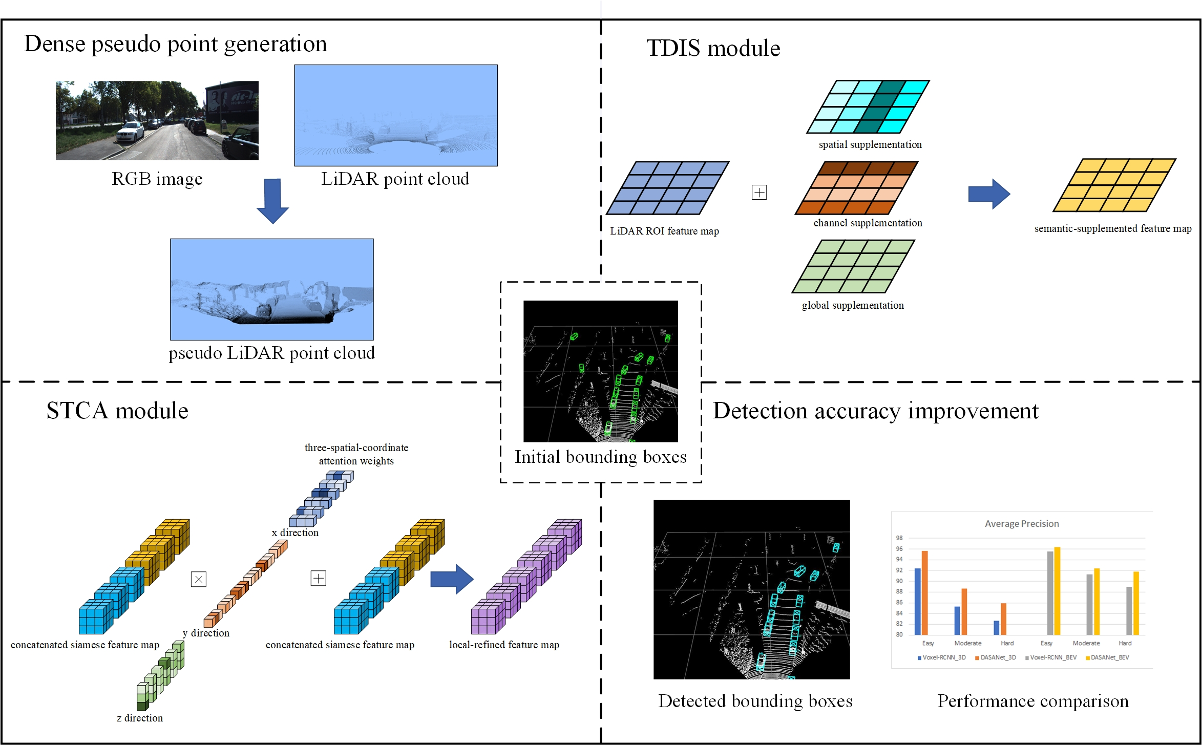
Remotesensing 15 04587 g001
Figure 2. Overview of the proposed DASANet, which is a 3D object detector with two stages. In the first stage, given an RGB image, two groups of 3D feature maps are extracted from the corresponding LiDAR point cloud and the generated pseudo-LiDAR point cloud to obtain the initial proposals. In the second stage, the proposed TDIS module and the STCA module are used to obtain fused features with more abundant semantic representation and the detailed information for 3D object detection. The overall process of the DASANet is summarized in Algorithm A1 in Appendix A.
Remotesensing 15 04587 g002
Figure 3. Overview of the TDIS module. First, the element subtraction of F P from F S , whose spatial direction is the spatial dimension flattening result of the 3D feature map along the channel dimension, is used to obtain differential feature map F D . Then, semantic feature maps F S p , F C h , and F G o are computed using the feature enhancement operations with weights W S p , W C h , and W G o . Finally, the feature supplementation operation is implemented using the spatial-dimension, channel-dimension, and all-element sum of F D and F S p , F C h , and F G o to obtain the semantic-supplemented feature map F T .
Remotesensing 15 04587 g003
Figure 4. Overview of the STCA module, which consists of two parts (a Siamese sparse encoder and a three-dimension coordinate attention). With P S and P P as inputs, the Siamese sparse encoder outputs the feature maps F E S and F E P . Then, the concatenated feature map F C is input into the TCA to obtain the local-refined feature map F A .
Remotesensing 15 04587 g004
Figure 5. Pipeline of the TCA. In the squeeze step, α X , α Y , and α Z are output by the global average pooling along the x direction, y direction, and z direction, respectively, maintaining their channel dimensions. Then, two convolution operations are used to obtain the attention weights corresponding to three spatial coordinates, i.e., g X , g Y , and g Z . Finally, the feature of each spatial location is weighted along the channels to obtain the local-refined feature map F A .
Remotesensing 15 04587 g005
Figure 6. The structure of the auxiliary head. The auxiliary head consists of three two-layer MLPs. The one-dimension vectors flattened from F T and F A are input into the shared two-layer MLP whose output size is 256. The parallel two-layer MLPs are used to generate the class label and the regression parameters of the bounding boxes.
Remotesensing 15 04587 g006
Figure 7. Visualization comparison of the proposed DASANet and the Voxel-RCNN in a complex-background situation.
Remotesensing 15 04587 g007
Figure 8. Visualization comparison of the proposed DASANet and the Voxel-RCNN in a long-distance situation.
Remotesensing 15 04587 g008
Figure 9. Visualization comparison of the proposed DASANet and the Voxel-RCNN in an occlusion situation.
Remotesensing 15 04587 g009
Figure 10. Visualization comparison of the proposed DASANet and the Voxel-RCNN in a large scene. Green boxes, blue boxes, and yellow boxes indicate the ground-truth, the DASANet prediction, and the Voxel-RCNN prediction, respectively.
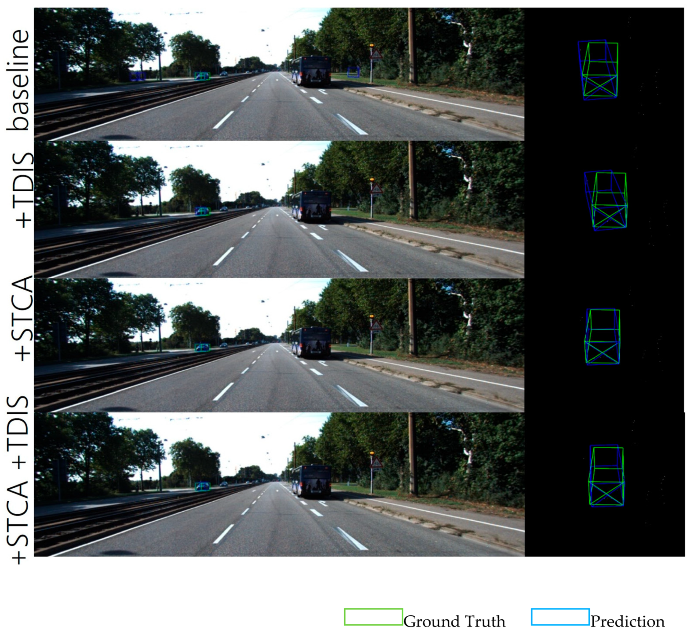
Remotesensing 15 04587 g010
Figure 11. Visualization ablation comparison between the baseline, +TDIS, +STCA and +TDIS +STCA.
Remotesensing 15 04587 g011
Table 1. Car 3D detection performance of different networks using the KITTI validation set. In modality, L denotes LiDAR, L + C denotes LiDAR and camera, and - denotes that the corresponding metric is not provided by the original paper.
NetworksModalityAP3D11AP3D40
EasyModerateHardEasyModerateHard
SECONDL88.6178.6277.22---
PointPillarsL86.6276.0668.91---
PointRCNNL88.8878.6377.38---
SA-SSDL90.1579.9178.78---
PV-RCNNL---92.5784.8382.69
Voxel-RCNNL89.4184.5278.9392.3885.2982.26
Pyramid-RCNNL89.3784.3878.84---
MV3DL + C86.5578.1076.67---
PointPaintingL + C88.3877.7476.76---
F-PointNetL + C83.7670.9263.65---
Focals ConvL + C---92.2685.3282.95
CLOCsL + C---92.7885.9483.25
VFFL + C89.5184.7679.2192.4785.6583.38
FusionRCNNL + C89.9086.4579.32---
SFDL + C89.7487.1285.2095.4788.5685.74
DASANetL + C90.6986.5285.4895.6388.6885.87
Table 2. Car BEV detection performance of different networks using the KITTI validation set. In modality, L denotes LiDAR, L + C denotes LiDAR and camera, and - denotes that the corresponding metric is not provided by the original paper.
NetworksModalityAPBEV11APBEV40
EasyModerateHardEasyModerateHard
SECONDL89.9687.0779.66---
PointPillarsL88.3586.1079.83---
PointRCNNL89.7886.1985.02---
SA-SSDL---95.0391.0385.96
PV-RCNNL---95.7691.1188.93
Voxel-RCNNL---95.5291.2588.99
MV3DL + C86.5578.1076.67---
F-PointNetL + C88.1684.9276.4491.1784.6774.77
Focals ConvL + C---94.4591.5191.21
CLOCsL + C---93.0589.8086.57
VFFL + C---95.6591.7591.39
SFDL + C---96.2492.0991.32
DASANetL + C90.5089.2688.5896.3992.4291.77
Table 3. Car 3D and BEV detection performance of different networks using the KITTI test set. In modality, L denotes LiDAR, L + C denotes LiDAR and camera. The best results are bolded. - means that the data was not provided by the original paper.
NetworksModalityAP3D40APBEV40
EasyModerateHardEasyModerateHard
SECONDL85.2976.6071.7790.9887.4884.22
PointPillarsL82.5874.3168.9990.0786.5682.81
PointRCNNL86.9675.6470.7092.1387.3982.72
SA-SSDL88.7579.7974.1695.0391.0385.96
PV-RCNNL90.2581.4376.8294.9890.6586.14
Voxel-RCNNL90.9081.6277.0694.8588.8386.13
Pyramid-RCNNL88.3982.0877.4992.1988.8486.21
MV3DL + C74.9763.6354.0086.6278.9369.80
PointPaintingL + C82.1171.7067.0892.4588.1183.36
F-PointNetL + C82.1969.7960.5991.1784.6774.77
Focals ConvL + C90.5582.2877.5992.6789.0086.33
CLOCsL + C89.1682.2877.2392.2189.4886.42
VFFL + C89.5082.0979.29---
FusionRCNNL + C88.1281.9677.53---
SFDL + C91.7384.7677.9295.6491.8586.83
DASANetL + C91.7784.9880.2195.5091.6988.89
Table 4. Comparison of ablation performance using the KITTI validation set. The improvement denotes the difference from the baseline.
NetworksAP3D40APBEV40
EasyModerateHardEasyModerateHard
Baseline92.3885.2982.6695.5291.2588.99
+TDIS93.3186.1583.6096.4891.9389.51
Improvement+0.93+0.86+0.94+0.96+0.68+0.52
+STCA93.5886.1685.0696.5791.8191.24
Improvement+1.20+0.87+2.40+1.05+0.56+2.25
+TDIS +STCA95.6388.6885.8796.3992.4291.77
Improvement+3.25+3.39+3.21+0.87+1.17+2.78
Table 5. Ablation comparisons of computational load and inference speed on the KITTI validation set.
NetworksParams (M)FLOPs (G)FPS (Hz)
baseline6.922.725.2
+TDIS26.228.014.5
+STCA30.827.912.7
+TDIS +STCA55.230.910.5
Table 6. Comparisons using the KITTI validation set for different distances. The improvement denotes the difference from the baseline.
NetworksAP3D40APBEV40
0 m–20 m20 m–40 m40 m-Inf0 m–20 m20 m–40 m40 m-Inf
Baseline92.1174.9913.8595.4986.5025.64
+TDIS +STCA95.0178.9122.2798.0588.0535.14
Improvement+2.90+3.92+8.42+2.56+1.55+9.50
Table 7. Comparisons using the KITTI validation set for different occlusion levels. Level 0, 1, and 2 denote that the object is fully visible, the object is partly occluded, and the object is difficult to see, respectively. The improvement denotes the difference from the baseline.
NetworksAP3D40APBEV40
Level 0Level 1Level 2Level 0Level 1Level 2
Baseline54.7067.4051.5957.6674.6864.97
+TDIS +STCA55.2969.6656.2958.1077.6868.20
Improvement+0.59+2.26+4.70+0.44+3.00+3.23
Table 8. Comparisons using the KITTI validation set for different numbers of points in the GT bounding boxes. points. The improvement denotes the difference from the baseline.
NetworksAP3D40APBEV40
<100p100 p–200 p>200 p<100 p100 p–200 p>200 p
Baseline40.9875.1895.3553.1384.9297.71
+TDIS +STCA56.5785.3896.9656.5790.8798.19
Improvement+15.59+10.20+1.61+3.44+5.95+0.48
Disclaimer/Publisher’s Note: The statements, opinions and data contained in all publications are solely those of the individual author(s) and contributor(s) and not of MDPI and/or the editor(s). MDPI and/or the editor(s) disclaim responsibility for any injury to people or property resulting from any ideas, methods, instructions or products referred to in the content.

