Optimizing an Algorithm Designed for Sparse-Frequency Waveforms for Use in Airborne Radars

Abstract

Low-frequency bands are an important way to realize stealth target detection for airborne radars. However, in a complex electromagnetic environment; when low-frequency airborne radar operates over land, it will inevitably encounter a lot of unintentional communication and intentional interference, while effective suppression of interference can not be achieved only through the adaptive processing of the receiver. To solve this problem, this paper proposes optimizing an algorithm designed for sparse-frequency waveforms for use in airborne radars. The algorithm establishes a joint objective function based on the criteria of minimizing waveform energy in the spectrum stopband and minimizing the integrated sidelobe level of specified range cells. The waveform is optimized by a cyclic iterative algorithm based on the Fast Fourier Transform (FFT) operation. It can ensure the frequency domain stopband constraint to realize the effective suppression of main-lobe interference while forming lower-range sidelobes at specified range cells to improve the ability to detect dim targets. Theoretical analysis and simulation results have shown that the algorithm has good anti-interference performance.

1. Introduction

The appearance of stealth aircraft, such as the F-22 and F-35, has brought serious challenges to airborne early warning radar systems that take conventional targets as detection objects. Low-frequency bands are an internationally recognized effective means of stealth detection, yet the low-frequency band spectrum is very crowded, and there are a large number of radiation sources, which are especially dense over land [1], resulting in the widespread existence of main lobe interference in low-frequency-band airborne early warning radars. Thus, effective suppression of dense main lobe interference can not be achieved only through the adaptive processing of the receiver.

Cognitive radars can obtain information by sensing the battlefield environment and feeding it back to the transmitter, thereby changing the traditional one-way processing mode of the radar and forming a new architecture of a dynamic closed loop between the receiver, the transmitter, and the battlefield environment [2,3,4,5]. The processing information in the different stages flows into the closed loop, and finally achieves the goal of enhancing the performance of the radar system [6,7,8]. The cycle of information begins with the transmitter broadcasting signals to illuminate the surrounding environment. After the radar receives the signal and the signal enters the receiver, the scene analyzer extracts the target information and environmental information required to judge the target and environmental status. The intelligent decision center controls the transmitter resources based on the information provided by the scene analyzer. The transmitter adjusts the transmitted waveform parameters to adapt to the environment based on the decision results [9,10,11].

Cognitive waveform design is a core and key technology in cognitive radars [12,13,14,15]. The key is how to use the knowledge of the target/interference characteristics to maximize the extraction of interesting target information in strong-interference environments [16,17,18]. This technology adaptively changes the transmitted waveform parameters by using prior environmental information to generate a sparse-frequency waveform with a spectrum stopband and transmit a waveform with good low-autocorrelation sidelobes, which improves the anti-interference ability and dim-target detection ability of the radar [19,20,21]. There has been a lot of work in the past decade on sparse recovery applications [22,23,24], which has resulted in sparse recovery technology being applied in many fields [25,26,27].

Spectrum constraint is the application of prior information to impose constraints on the frequency bands that interfere or conflict with other radar and communication equipment. These form notches at the corresponding positions to suppress interference or avoid conflicts to finally obtain a sparse-frequency waveform. An algorithm designed for sparse-frequency waveforms based on the steepest descent (SD) was proposed in [28], which forms notches at the interference frequency bands to suppress interference and reduces the range sidelobes through time–domain mismatch filters; however, this algorithm requires a lot of computation and will cause mismatch losses. The genetic algorithm (GA) proposed in [29] and the particle swarm optimization (PSO) proposed in [30] are both stochastic evolutionary algorithms. When these algorithms are used to solve the objective function, the search direction is arbitrary, and the iterative steps are long. Moreover, the computation is large, and the convergence speed is slow. In [31], weight coefficients were introduced to establish a joint objective function, balance the performance of Power Spectral Density (PSD) and autocorrelation function (ACF), and extend the algorithm to the MIMO radar. In [32], detector design and performance analysis of target detection in subspace interference were proposed.

In addition to the sparse-frequency-waveform design, another important aspect of cognitive waveform technology is the design of transmitted waveforms with low-range sidelobes. The reason is that if, after matched filtering, the output signal of the radar waveform has a high-autocorrelation sidelobe level and some range cells have sidelobe interference, such as from strong clutters, multipath interferences, and sea clutter spikes, the detection of dim targets will be seriously affected. The CAN algorithm proposed in [33] uses the minimum integrated sidelobe level (ISL) as the optimization criterion. The algorithm is based on the Fast Fourier Transform (FFT) and optimizes the waveform design to suppress all range sidelobes, although it does not consider the sidelobe suppression of specified range cells, and also lacks some pertinence. The WeCAN [33] algorithm, based on the minimum weighted integrated sidelobe level (WISL), can form an extremely low sidelobe at the specified range of cells by using prior information, which has a more significant suppression effect and significantly improves the detection performance of the radar. However, compared to the CAN algorithm, the computational complexity of this algorithm is increased. The WeSCAN algorithm proposed in [34] can generate sequences with a deeper frequency stopband notch, although at the cost of increasing the width of the main lobe, which introduces the disadvantage of increasing the computational complexity. Designing an algorithm for sparse-frequency waveform optimization under the range of sidelobe level constraints proposed in [35] sets the PSD of the expected waveform as a 0–1 weighted vector. Its disadvantage is that the PSD value is uniformly set to 1 in the spectrum passband, and the stopband depth is not adjustable.

In order to achieve effective suppression of dense main lobe interference and improve the ability to detect dim targets, an algorithm for designing sparse-frequency waveforms for airborne radar based on waveform energy minimization in the stopband was proposed in this paper, namely, Stopband waveform energy Minimization Iterative Algorithm (SMIA). In the frequency domain, the objective function is established through an optimization criterion of minimum wave energy in the frequency stopband. Then, a new autocorrelation function sequence is formed by the relationship between the waveform autocorrelation function and power spectrum density, and the problem of integrated sidelobe level minimization of a specified range cells is converted into a power spectrum density fitting problem. Then, the weighting factor is employed to form a new objective function. Finally, the waveform is optimized by the circular iterative algorithm based on an FFT operation. Compared with traditional waveform-optimization design algorithms, the stopband depth of the proposed algorithm can be adjusted while keeping the stopband constraint in the frequency domain, and lower range sidelobes can be formed at specified range cells. Meanwhile, the algorithm is optimized based on an FFT operation, and has relatively lower computational complexity.

2. Materials

It is assumed that the discrete signal form of the radar-transmitted waveform after N-point sampling is

$$\mathit{s}={[s_1\hspace{1em}{s}_2\hspace{1em}\cdots \begin{array}{c}\end{array}{s}_N]}^{\mathrm{T}}$$

(1)

The autocorrelation function of waveform s is defined as

$$r_k(\mathit{s})={\displaystyle \sum _{n=k+1}^N{s}_n{s}_{n-k}^{*}}=r_{-k}^{*}(\mathit{s}),\hspace{1em}k=0,1,\cdots ,N-1$$

(2)

where $r_0(\mathit{s})={\displaystyle \sum _{n=1}^N{s}_n{s}_n^{*}}$ is the waveform energy, $\{r_k(\mathit{s}), k=-N+1,\cdots ,-1,1,\cdots ,N-1\}$ represents the sidelobe of the waveform autocorrelation function, and the autocorrelation function of Equation (2) refers to the aperiodic autocorrelation function.

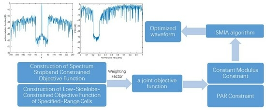
2.1. Construction of Spectrum Stopband Constrained Objective Function

Assume that the radar operating frequency band is $\left[{\phi }_{\min },{\phi }_{\max }\right]$, and the set of frequency stopbands of the waveform sequence is $\varphi =U_{l=1}^L\left[{\phi }_{l1},{\phi }_{l2}\right]$, where $\varphi \subseteq \left[{\phi }_{\min },{\phi }_{\max }\right]$, ${\phi }_{l1}$, and ${\phi }_{l2}$ represent the lower and upper bounds of the l-th stopband, respectively. Let $f={\left[f_1\begin{array}{c}\end{array}{f}_2\begin{array}{c}\end{array}\cdots \begin{array}{c}\end{array}{f}_K\right]}^{\mathrm{T}}$ represent the K-point Discrete Fourier Transform (DFT) of the transmitted waveform, where

$$\{\begin{array}{c}{f}_k={\displaystyle \sum _{n=1}^N{s}_n{e}^{-\mathrm{j}n{\omega }_k}}\\ {\omega }_k=\frac{2\pi }{K}k,\hspace{1em}k=1,2,\cdots ,K\end{array}$$

(3)

For the construction of the objective function of spectrum stopband constraint, the main purpose is to minimize the waveform energy in the frequency stopband so as to effectively suppress the interference from the same frequency band, that is, to minimize the waveform energy in $\varphi =U_{l=1}^L\left[{\phi }_{l1},{\phi }_{l2}\right]$.

In order to be consistent with the sequence length when constructing the low-sidelobe-constrained objective function of specified range cells in Section 2.2 below, here, let $K=2N$, that is, a 2N point PSD of the transmitted waveform $\mathit{s}$ is calculated by a 2N point DFT.

$$\begin{array}{ll}{f}_k& ={\displaystyle \sum _{n=1}^{2N}{s}_n{e}^{-\mathrm{j}n{\omega }_k}}\\ & =s_1{e}^{-\mathrm{j}{\omega }_k}+s_2{e}^{-\mathrm{j}2{\omega }_k}+\cdots +s_{2N}{e}^{-\mathrm{j}2N{\omega }_k}\\ & =\left[e^{-\mathrm{j}{\omega }_k}\begin{array}{c}\end{array}{e}^{-\mathrm{j}2{\omega }_k}\begin{array}{c}\end{array}\cdots \begin{array}{c}\end{array}{e}^{-\mathrm{j}2N{\omega }_k}\right]\cdot {\left[{\mathit{s}}^T\begin{array}{c}\end{array}{\mathbf{0}}_{1\times N}\right]}^{\mathrm{T}}\\ & ={\mathit{a}}_k\mathit{y}\end{array}$$

(4)

where ${\mathit{a}}_k=\left[e^{-\mathrm{j}{\omega }_k}\hspace{1em}{e}^{-\mathrm{j}2{\omega }_k}\hspace{1em}\cdots \hspace{1em}{e}^{-\mathrm{j}2N{\omega }_k}\right]$, $\mathit{y}={\left[{\mathit{s}}^{\mathrm{T}}\hspace{1em}{0}_{1\times N}\right]}^{\mathrm{T}}$ is a new 2N × 1-dimension sequence formed by adding N zeros after the sequence $\mathit{s}$, and ${(·)}^{\mathrm{T}}$ is the transpose operation.

Therefore, the 2N point PSD of the waveform sequence $\mathit{s}$ can be expressed as

$$\begin{array}{ll}f& ={\left[f_1\begin{array}{c}\end{array}{f}_2\begin{array}{c}\end{array}\cdots \begin{array}{c}\end{array}{f}_{2N}\right]}^{\mathrm{T}}\\ & ={\left[{\mathit{a}}_1{\left[{\mathit{s}}^T\begin{array}{c}\end{array}{\mathbf{0}}_{1\times N}\right]}^{\mathrm{T}}\begin{array}{c}\end{array}{\mathit{a}}_2{\left[{\mathit{s}}^T\begin{array}{c}\end{array}{\mathbf{0}}_{1\times N}\right]}^{\mathrm{T}}\begin{array}{c}\end{array}\cdots \begin{array}{c}\end{array}{\mathit{a}}_{2N}{\left[{\mathit{s}}^T\begin{array}{c}\end{array}{\mathbf{0}}_{1\times N}\right]}^{\mathrm{T}}\right]}^{\mathrm{T}}\\ & =\left[\begin{array}{c}{\mathit{a}}_1\\ {\mathit{a}}_2\\ ⋮\\ {\mathit{a}}_{2N}\end{array}\right]\cdot {\left[{\mathit{s}}^T\begin{array}{c}\end{array}{\mathbf{0}}_{1\times N}\right]}^{\mathrm{T}}\\ & =\mathbf{F}\cdot \mathit{y}\end{array}$$

(5)

where $\mathbf{F}$ is a 2N × 2N FFT transformation matrix.

To obtain the power spectrum density with the minimum waveform energy in the frequency stopband, the objective function can be constructed by introducing the weighting coefficient, where the weighted vector $\mathit{w}$ can be obtained by prior information [36]. $w_k=0$ for the passband while $w_k\in \left(0,1\right]$ for the stopband, where $w_k\in \left(0,1\right]$ means taking a value within the range of (0,1] and then adjusting the stopband depth; $w_k$ represents the value of the k-th frequency point. The weight vector $\mathit{w}$ is

$$\mathit{w}={\left[w_1,w_2,\cdots ,w_{2N}\right]}^{\mathrm{T}}$$

(6)

Then, the objective function of the minimum waveform energy in the frequency stopband is

$$\underset{\mathit{s}}{\min }\begin{array}{c}\end{array}{\Vert {\tilde{\mathbf{G}}}^{\mathrm{H}}\mathit{y}\Vert }^2$$

(7)

where ${(·)}^{\mathrm{H}}$ is the conjugate transpose operation, the matrix $\tilde{\mathbf{G}}={\mathbf{F}}^{\mathrm{H}}\mathrm{diag}\left(\mathit{w}\right)$, and $\mathrm{diag}(·)$ is the diagonal matrix.

If y is in the null space of ${\tilde{\mathbf{G}}}^{\mathrm{H}}$, then the value of Equation (7) is 0. Since the null space of ${\tilde{\mathbf{G}}}^{\mathrm{H}}$ can be represented by the columns of matrix G, Equation (7) can be converted to

$$\underset{\mathit{s}}{\min }\begin{array}{c}\end{array}{\Vert \mathit{y}-\mathbf{G}\mathit{v}\Vert }^2$$

(8)

where $\mathbf{G}=\frac{1}{2N}{\mathbf{F}}^{\mathrm{H}}\mathrm{diag}\left(\tilde{\mathit{w}}\right)$, $\tilde{\mathit{w}}=\mathbf{D}-\mathit{w}$, $\mathbf{D}$ is a matrix with the dimension of 2N × 1 and elements are 1. $\mathit{v}$ is a 2N × 1-dimensional auxiliary optimization variable.

Because $\mathbf{F}{\mathbf{F}}^{\mathrm{H}}/2N={\mathbf{F}}^{\mathrm{H}}\mathbf{F}/2N=I$, by substituting the matrix $\mathbf{G}$, Equation (8) can be rewritten as

$$\underset{\mathit{s}}{\min }\begin{array}{c}\end{array}{\Vert \mathbf{F}\mathit{y}-\mathrm{diag}\left(\tilde{\mathit{w}}\right)\mathit{v}\Vert }^2$$

(9)

2.2. Construction of Low-Sidelobe-Constrained Objective Function of Specified-Range Cells

There is another mathematical model of the minimum waveform energy in the spectrum stopband:

$$\underset{\mathit{s}}{\min }\begin{array}{c}\end{array}{\Vert \mathit{f}\odot \mathit{f}\Vert }^2$$

(10)

Since the autocorrelation function sequence of waveform and waveform PSD are Fourier transform pairs, a new autocorrelation function sequence $\mathit{m}\left(\mathit{s}\right)$ can be constructed [37] (See Appendix A for details).

$$\mathit{m}\left(\mathit{s}\right)={\left[r^0\right(\mathit{s})\hspace{1em}{r}^1(\mathit{s})\cdots r_{N-1}(\mathit{s})\hspace{1em}0\hspace{1em}{r}_{N-1}^{*}(\mathit{s})\hspace{1em}{r}_{N-2}^{*}(\mathit{s})\cdots r_1^{*}(\mathit{s}\left)\right]}^{\mathrm{T}}$$

(11)

Assuming that the ideal autocorrelation function sequence is $\mathit{m}\left(\tilde{\mathit{s}}\right)$, where $\tilde{\mathit{s}}$ is the ideal waveform, and the minimum mean square error criterion is used to make the final optimized waveform $\mathit{s}$ to the ideal waveform $\tilde{\mathit{s}}$, then the objective function is

$$\underset{\mathit{s}}{\min }\begin{array}{c}\end{array}{\Vert \mathit{m}\left(\mathit{s}\right)-\mathit{m}\left(\tilde{\mathit{s}}\right)\Vert }^2$$

(12)

It is assumed that the relevant information of the ideal waveform $\tilde{\mathit{s}}$ can be obtained from prior information, that is, the low sidelobe information of specified-range cells is known. Then, the new autocorrelation function is processed in the way of 0–1 weighting, $z_k=0$ for the region that needs to be suppressed, and $z_k=1$ for the region that does not need to be suppressed, where $z_k$ represents the value of the k-th cell.

Therefore, the ideal autocorrelation function sequence $\mathit{m}\left(\tilde{\mathit{s}}\right)$ can be expressed as

$$\mathit{m}\left(\tilde{\mathit{s}}\right)=\mathit{m}\left(\mathit{s}\right)\odot {\mathit{w}}_{\mathrm{s}}$$

(13)

where ${\mathit{w}}_{\mathrm{s}}$ is the weight vector in the same order as the new autocorrelation function sequence

$${\mathit{w}}_{\mathrm{s}}={\left[z_0,z_1,\cdots ,z_{N-1}\hspace{1em}0\hspace{1em}{z}_{N-1}^{*},\cdots ,z_1^{*}\right]}^{\mathrm{T}}$$

(14)

Convert Equation (10) to matrix form as follows:

$$\begin{array}{ll}f\odot f^{*}& ={\left[f_1\cdot f_1^{*}\begin{array}{c}\end{array}{f}_2\cdot f_2^{*}\begin{array}{c}\end{array}\cdots \begin{array}{c}\end{array}{f}_{2N}\cdot f_{2N}^{*}\right]}^{\mathrm{T}}\\ & ={\left[{\mathit{a}}_1\mathit{y}{\left({\mathit{a}}_1\mathit{y}\right)}^{*}\begin{array}{c}\end{array}{\mathit{a}}_2\mathit{y}{\left({\mathit{a}}_2\mathit{y}\right)}^{*}\begin{array}{c}\end{array}\cdots \begin{array}{c}\end{array}{\mathit{a}}_{2N}\mathit{y}{\left({\mathit{a}}_{2N}\mathit{y}\right)}^{*}\right]}^{\mathrm{T}}\\ & =\left(\mathbf{F}\mathit{y}\right)\odot \left({\mathbf{F}}^{*}{\mathit{y}}^{*}\right)\end{array}$$

(15)

where $\mathbf{F}$ is a 2N × 2N FFT transformation matrix, and $\mathit{y}$ is ${\left[{\mathit{s}}^T\begin{array}{c}\end{array}{\mathbf{0}}_{1\times N}\right]}^{\mathrm{T}}$.

From Appendix A, ${\mathit{\beta }}_k=\left[1\begin{array}{c}\end{array}{e}^{-\mathrm{j}{\omega }_k}\begin{array}{c}\end{array}{e}^{-\mathrm{j}2{\omega }_k}\begin{array}{c}\cdots \begin{array}{c}\end{array}{e}^{-\mathrm{j}(N-1){\omega }_k}\begin{array}{c}\end{array}\end{array}{e}^{-\mathrm{j}N{\omega }_k}\begin{array}{c}\end{array}{e}^{-\mathrm{j}(N+1){\omega }_k}\cdots \begin{array}{c}\end{array}{e}^{-\mathrm{j}(2N-1){\omega }_k}\right]$, $f_k\cdot f_k^{*}={\mathit{\beta }}_k\mathit{m}\left(\mathit{s}\right)$

$$\begin{array}{ll}f\odot f^{*}& ={\left[f_1\cdot f_1^{*}\begin{array}{c}\end{array}{f}_2\cdot f_2^{*}\begin{array}{c}\end{array}\cdots \begin{array}{c}\end{array}{f}_{2N}\cdot f_{2N}^{*}\right]}^{\mathrm{T}}\\ & ={\left[{\mathit{\beta }}_1\mathit{m}\left(\mathit{s}\right)\begin{array}{c}\end{array}{\mathit{\beta }}_{2N}\mathit{m}\left(\mathit{s}\right)\begin{array}{c}\end{array}\cdots \begin{array}{c}\end{array}{\mathit{\beta }}_1\mathit{m}\left(\mathit{s}\right)\right]}^{\mathrm{T}}\\ & =\mathbf{B}\mathit{m}\left(\mathit{s}\right)\end{array}$$

(16)

where $\mathit{B}$ is ${\left[{\mathit{\beta }}_1^{\mathrm{T}}\begin{array}{c}\end{array}{\mathit{\beta }}_2^{\mathrm{T}}\begin{array}{c}\end{array}\cdots \begin{array}{c}\end{array}{\mathit{\beta }}_{2N}^{\mathrm{T}}\right]}_{2N\times 2N}^{\mathrm{T}}$.

According to Equation (15), Equation (16), and $\mathbf{B}{\mathbf{B}}^{\mathrm{H}}/2N={\mathbf{B}}^{\mathrm{H}}\mathbf{B}/2N=\mathbf{I}$, it can be concluded that

$$\mathit{m}\left(\mathit{s}\right)={\mathbf{B}}^{\mathrm{H}}\left(\mathbf{F}\mathit{y}\right)\odot \left({\mathbf{F}}^{*}{\mathit{y}}^{*}\right)/2N$$

(17)

Equation (12) can be rewritten as

$$\underset{\mathit{s}}{\min }\begin{array}{c}\end{array}{\Vert \mathbf{B}\mathit{m}\left(\mathit{s}\right)-\mathbf{B}\left(\mathit{m}\left(\mathit{s}\right)\odot {\mathit{w}}_{\mathrm{s}}\right)\Vert }^2$$

(18)

In Equation (18), $\mathbf{B}\mathit{m}\left(\mathit{s}\right)$ represents the PSD of the waveform $\mathit{s}$ to be optimized, and $\mathbf{B}\left(\mathit{m}\left(\mathit{s}\right)\odot {\mathit{w}}_{\mathrm{s}}\right)$ represents the PSD of the expected waveform $\tilde{\mathit{s}}$. Therefore, the objective function is transformed from the original waveform approximation problem to a waveform PSD fitting problem.

Expand each term of Equation (18) to

$$\mathbf{B}\mathit{m}\left(\mathit{s}\right)=\left(\mathbf{F}\mathit{y}\right)\odot \left({\mathbf{F}}^{*}{\mathit{y}}^{*}\right)$$

(19)

$$\mathbf{B}\left(\mathit{m}\left(\mathit{s}\right)\odot {\mathit{w}}_{\mathrm{s}}\right)=\tilde{\mathit{g}}\odot {\tilde{\mathit{g}}}^{*}$$

(20)

where $\mathbf{F}\mathit{y}$ is the spectrum of the actual waveform, $\tilde{\mathit{g}}$ is the spectrum of the ideal waveform, and the objective function of Equation (18) can be expressed as the spectrum fitting function, namely

$$\underset{\mathit{y}}{\min }\begin{array}{c}\end{array}{\Vert \left(\mathbf{F}\mathit{y}\right)\odot \left({\mathbf{F}}^{*}{\mathit{y}}^{*}\right)-\tilde{\mathit{g}}\odot {\tilde{\mathit{g}}}^{*}\Vert }^2$$

(21)

Introducing phase assist vector

$$\mathit{u}={\left[e^{\mathrm{j}{\theta }_1}\begin{array}{c}\end{array}\cdots \begin{array}{c}\end{array}{e}^{\mathrm{j}{\theta }_{2N}}\right]}_{2N\times 1}^{\mathrm{T}}$$

(22)

Equation (21) can be converted to

$$\underset{\mathit{s},\mathit{u}}{\min }\begin{array}{c}\end{array}{\Vert \mathbf{F}(\mathbf{T}\mathit{s})-\mathit{h}\odot \mathit{u}\Vert }^2$$

(23)

where $\mathit{h}=\sqrt{\left|\mathbf{B}\left(\mathit{m}\left(\mathit{s}\right)\odot {\mathit{w}}_{\mathrm{s}}\right)\right|}$ is the amplitude of the ideal spectrum, $\sqrt{|·|}$ represents the square root of the absolute value of each element in the vector, and $\mathbf{T}={\left[{\mathbf{I}}_N\begin{array}{c}\end{array}{\mathbf{0}}_N\right]}_{2N\times N}^{\mathrm{T}}$ is the zero-compensating matrix.

Combining Equation (9) and Equation (23), a weighting factor $\lambda$ is introduced to form a new objective function:

$$\underset{\mathit{s},\mathit{u},\mathit{v}}{\min }\begin{array}{c}\end{array}\lambda {\Vert \mathbf{F}{\left[{\mathit{s}}^T\hspace{1em}{\mathbf{0}}_{1\times N}\right]}^{\mathrm{T}}-\mathrm{diag}\left(\tilde{\mathit{w}}\right)\mathit{v}\Vert }^2+\left(1-\lambda \right){\Vert \mathbf{F}(\mathbf{T}\mathit{s})-\mathit{h}\odot \mathit{u}\Vert }^2$$

(24)

It should be noted that matrix $\mathbf{F}$, matrix $\mathbf{B}$, matrix $\mathbf{T}$, vector $\tilde{\mathit{w}}$, and vector $\mathit{h}$ are known, and the objective function contains $\mathit{s}$, $\mathit{u}$, $\mathit{v}$, three variables, and the optimal solution of the third variable can be obtained by fixing two variables and then iteratively solving it continuously.

3. Optimization Algorithm

3.1. Optimization Algorithm under Constant Modulus Constraint

In order to maximize the utilization of transmitter power and avoid nonlinear distortion of the output waveform, constant modulus constraints are usually added in the waveform design process [38], where the objective function becomes

$$\begin{array}{l}\underset{\mathit{s},\mathit{u},\mathit{v}}{\min }\begin{array}{c}\end{array}\lambda {\Vert \mathbf{F}{\left[{\mathit{s}}^T\begin{array}{c}\end{array}{\mathbf{0}}_{1\times N}\right]}^{\mathrm{T}}-\mathrm{diag}\left(\tilde{\mathit{w}}\right)\mathit{v}\Vert }^2+\left(1-\lambda \right){\Vert \mathbf{F}(\mathbf{T}\mathit{s})-\mathit{h}\odot \mathit{u}\Vert }^2\\ \mathrm{s}.\mathrm{t}.\begin{array}{c}\end{array}\left|s_k\right|=1,\begin{array}{c}\end{array}1\le k\le N\end{array}$$

(25)

The main idea of solving the objective function is to assume that $\mathit{s}$ and $\mathit{u}$ are known and minimize Equation (25) to obtain the optimal solution of $\mathit{v}$; then, assuming that $\mathit{s}$ and $\mathit{v}$ are known, the optimal solution of $\mathit{u}$ is obtained. Then, $\mathit{u}$ and v are updated, the optimal solution of $\mathit{s}$ is obtained, and the iterative cycle continues until the preset stopping condition $\Vert {\mathit{s}}^{(i)}-{\mathit{s}}^{(i+1)}\Vert <\epsilon$ is met, where ${\mathit{s}}^{(i)}$ is the sequence obtained by the i-th iteration and $\epsilon$ is the preset threshold.

When $\mathit{s}$ and $\mathit{u}$ are known, the optimal solution of $\mathit{v}$ is

$$\mathit{v}=\mathbf{F}{\left[{\mathit{s}}^{\mathrm{T}}\begin{array}{c}\end{array}{0}_{1\times N}\right]}^{\mathrm{T}}\odot \tilde{\mathit{w}}$$

(26)

When $\mathit{s}$ and $\mathit{v}$ are known, the optimal solution of $\mathit{u}$ is

$$\mathit{u}=e^{\mathrm{j}\arg \left\{\mathbf{F}\left(\mathbf{T}\mathbf{s}\right)\right\}}$$

(27)

When $\mathit{u}$ and $\mathit{v}$ are given, the objective function can be written as

$$\mathrm{const}-2\mathrm{Re}\left\{{\mathit{s}}^{\mathrm{H}}\left[\lambda {\mathit{c}}_1+\left(1-\lambda \right){\mathit{c}}_2\right]\right\}$$

(28)

where $\mathrm{const}$ is the constant term independent of $\mathit{s}$, ${\mathit{c}}_1$ is the first N elements of ${\mathbf{F}}^{\mathrm{H}}\mathit{v}\odot \tilde{\mathit{w}}$, and ${\mathit{c}}_2$ is the first N elements of ${\mathbf{F}}^{*}\left(\mathit{h}\odot \mathit{u}\right)$.

Then, the optimal solution of $\mathit{s}$ is

$$\mathit{s}=\exp \left\{\mathrm{j}\arg \left[\lambda {\mathit{c}}_1+\left(1-\lambda \right){\mathit{c}}_2\right]\right\}$$

(29)

Continuously iterate until convergence.

The specific steps of the SMIA algorithm under constant modulus constraint are provided as follows (Algorithm 1).

Algorithm 1: SMIA algorithm under constant modulus constraint

Input: randomly initialize the sequence $\mathit{s}$;

Step 1: For the current sequence $\mathit{s}$ and u, calculate the optimal solution of $\mathit{v}$ (see Equation (26));

Step 2: For the current sequence s and $\mathit{v}$, calculate the optimal solution of $\mathit{u}$ (see Equation (27));

Step 3: For the current sequence $\mathit{u}$ and $\mathit{v}$, calculate the optimal solution of $\mathit{s}$ (see Equation (29));

Step 4: Iterate through Step 1, Step 2, and Step 3 until the preset stop condition $\Vert {\mathit{s}}^{(i)}-{\mathit{s}}^{(i+1)}\Vert <\epsilon$ is met;

Output: the final optimized waveform ${\mathit{s}}^{(i)}$.

3.2. Optimization Algorithm under PAR Constraint

From the point of view of maximization of transmitter power, the ideal transmission waveform can be obtained under constant modulus constraint, but the constraint is too harsh. The Peak-to-Average-power Ratio (PAR) constraint is a more general constraint than the constant modulus constraint, and its expression is

$$\mathrm{PAR}=\frac{{\Vert \mathit{s}\Vert }_{\infty }^2}{\frac{1}{N}{\Vert \mathit{s}\Vert }^2}\le \tau$$

(30)

The transmitted waveform meets the energy constraint, and ${\Vert \mathit{s}\Vert }^2=N$; the objective function under the PAR constraint is

$$\begin{array}{l}\underset{\mathit{s},\mathit{u},\mathit{v}}{\min }\begin{array}{c}\end{array}\lambda {\Vert \mathbf{F}{\left[{\mathit{s}}^T\begin{array}{c}\end{array}{\mathbf{0}}_{1\times N}\right]}^{\mathrm{T}}-\mathrm{diag}\left(\tilde{\mathit{w}}\right)\mathit{v}\Vert }^2+\left(1-\lambda \right){\Vert \mathbf{F}(\mathbf{T}\mathit{s})-\mathit{h}\odot \mathit{u}\Vert }^2\\ \mathrm{s}.\mathrm{t}.\begin{array}{c}\end{array}\left|s_k\right|\le \sqrt{\tau },\begin{array}{c}\end{array}1\le k\le N\end{array}$$

(31)

Similarly, the SMIA algorithm is used to solve the problem. When $\mathit{s}$ and $\mathit{u}$ are known, the optimal solution of v is

$$\mathit{v}=\mathbf{F}{\left[{\mathit{s}}^{\mathrm{T}}\hspace{1em}{0}_{1\times N}\right]}^{\mathrm{T}}\odot \tilde{\mathit{w}}$$

(32)

When $\mathit{s}$ and $\mathit{v}$ are known, the optimal solution of $\mathit{u}$ is

$$\mathit{u}=e^{\mathrm{j}\arg \left\{\mathbf{F}\left(\mathbf{T}\mathbf{s}\right)\right\}}$$

(33)

When $\mathit{u}$ and $\mathit{v}$ are known, according to reference [39], the Tropp alternate projection method is used to solve the problem. For $\overline{\mathit{s}}\triangleq {\mathbf{T}}^{\mathrm{T}}\left(\lambda {\mathbf{F}}^{\mathrm{H}}\mathit{v}\odot \tilde{\mathit{w}}+\left(1-\lambda \right){\mathbf{F}}^{*}\left(\mathit{h}\odot \mathit{u}\right)\right)$, if the magnitude of all elements in $\overline{\mathit{s}}$ is less than $\sqrt{\tau }$, then the optimal solution is $\mathit{s}=\sqrt{N}\left(\overline{\mathit{s}}/\Vert \overline{\mathit{s}}\Vert \right)$. Otherwise, the solution of the corresponding vector position of the element ${\overline{\mathit{s}}}_{\max }$ with the largest amplitude in $\overline{\mathit{s}}$ is $\sqrt{\tau }{e}^{\left(\mathrm{j}\arg \left({\overline{s}}_{\max }\right)\right)}$, and the solution of the corresponding vector position of the other elements can also be obtained by this algorithm and the waveform energy changes from $N$ to $N-\tau$.

The specific steps of the SMIA algorithm under the PAR constraint are provided as follows (Algorithm 2):

Algorithm 2: SMIA algorithm under the PAR constraint

Input: randomly initialize the sequence $\mathit{s}$; the waveform energy of $\mathit{s}$ is ${\Vert \mathit{s}\Vert }^2=N$, and the PAR constraint value is set to $\tau$;

Step 1: For the current sequence $\mathit{s}$ and $\mathit{u}$, calculate the optimal solution of $\mathit{v}$ (see Equation (32));

Step 2: For the current sequence $\mathit{s}$ and $\mathit{v}$, calculate the optimal solution of u (see Equation (33));

Step 3: For the current sequence $\mathit{u}$ and $\mathit{v}$, calculate the optimal solution of $\mathit{s}$ by the alternate projection method;

Step 4: Iterate through Step 1, Step 2, and Step 3 until the preset stop condition $\Vert {\mathit{s}}^{(i)}-{\mathit{s}}^{(i+1)}\Vert <\epsilon$ is met;

Output: the final optimized waveform.

4. Results

In this section, it is assumed that the waveform length N = 250; without loss of generality, the frequency is normalized, and its range is 0~1, the stop threshold of iterative convergence is set to 10⁻⁶, and the maximum number of iterations is 10⁴. If no special description is made, the spectrum uses a 0–1 weighted vector. In this section, the proposed SMIA algorithm is compared with the traditional WeSCAN algorithm under the constant modulus constraint and PAR constraint so as to verify the effectiveness of the proposed SMIA algorithm in reducing the sidelobes of specified-range cells and imposing spectrum constraint.

4.1. Comparisons under Constant Modulus Constraint

The autocorrelation function and the power spectral density obtained by the SMIA algorithm when $\lambda =0.9$ are shown in Figure 1; the frequency stopband is $[0.2,0.3)$ and the region of reducing the sidelobes of specified range cells is $k\in (3,50)$. The image obtained by the WeSCAN algorithm is shown in Figure 2, and other conditions are the same as those in Figure 1. By comparing Figure 1 and Figure 2, the average PSD notch depth of the SMIA algorithm is −30.12 dB, and the average PSD notch depth of the WeSCAN algorithm is −32.23 dB. The mean sidelobe of the specified-range cells autocorrelation function of the SMIA algorithm is −61.32 dB, and the mean sidelobe of the WeSCAN algorithm is −43.25 dB. It can be found that, when $\lambda =0.9$, that is, the stopband constraint weight is large, both the SMIA algorithm and WeSCAN algorithm can form a notch at the stopband, and the notch depth is basically the same; but, for the autocorrelation function sidelobe level of specified range cells, the SMIA algorithm can generate a lower range sidelobe than WeSCAN algorithm, with a difference of about 18 dB.

4.2. Comparisons under PAR Constraint

The autocorrelation function and power spectrum density of the SMIA algorithm and WeSCAN algorithm under the PAR constraint are shown in Figure 3 and Figure 4, respectively, where PAR ≤ 2 and other conditions are the same as in Section 4.1. It can be found that the results obtained by PAR constraint are consistent with those obtained by constant modulus constraint. However, due to the relaxation of the peak average ratio by PAR constraint, the degree of freedom of waveform design increases. Therefore, compared with the constant modulus constraint, the range sidelobe level obtained was relatively lower (about 20 dB lower), while the PSD spectrum constraint was less affected.

4.3. Anti-Interference Performance

In this experiment, the region of reducing the sidelobes of specified-range cells is $k\in (3,250)$ and the weighting factor is $\lambda =0.9$. In Figure 5, the transmitted waveform frequency stopband is $[0.2,0.3)$, the interference band is $(0.35,0.45)$, the interference-to-noise ratio is 15 dB, and the PSDs of the transmitted waveform and the interference waveform are shown in Figure 5a,b, respectively. Figure 5c is a PSD diagram of the echo waveform, including the transmitted waveform, interference waveform, and noise. Figure 5d shows the output of matched filtering between the echo waveform and the transmission waveform. It can be seen that the interference frequency band does not fall within the frequency stopband of the transmitted waveform, so the interference is not effectively suppressed after matched filtering. The simulation conditions in Figure 6 are essentially the same as those in Figure 5. The difference is that the frequency band of the interference waveform is $(0.22,0.28)$; this frequency band is in the frequency stopband of the transmitted waveform. Figure 6d shows the output after matched filtering. It can be found that the interference band falls within the frequency stopband of the transmitted waveform, and the interference is effectively suppressed after matched filtering because of the orthogonality of the frequency domain.

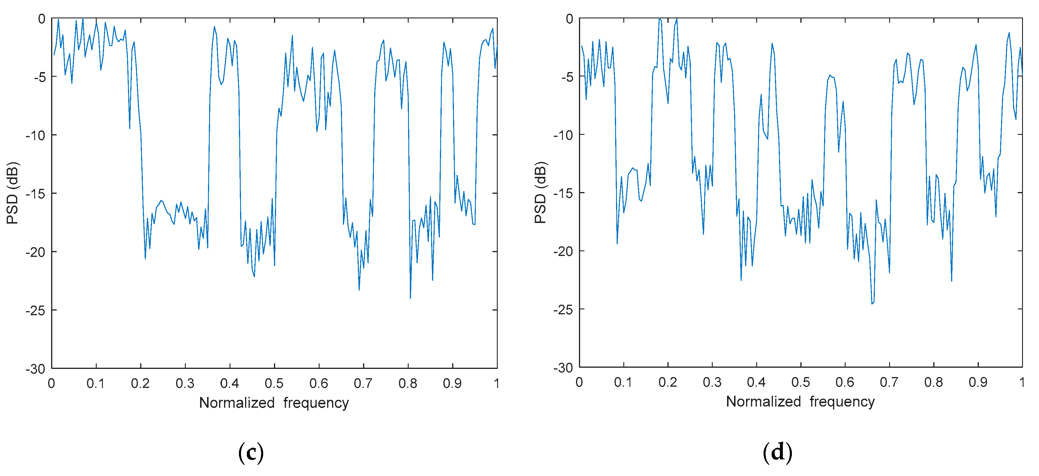
4.4. The Time–Frequency Distribution Characteristics of the Optimized Waveform

In order to clarify the time–frequency distribution characteristics of the waveform more clearly, this experiment assumes that the sequence length N = 1000. The frequency stopband is [0.08, 0.16) U [0.25, 0.3) U [0.35, 0.4) U [0.45, 0.55) U [0.6, 0.7) U [0.78, 0.85) U [0.9, 0.95). The time–frequency distribution of the optimized waveform obtained by the SMIA algorithm is shown in Figure 7. It can be seen from the figure that the spectrum power of the final optimized waveform is evenly distributed in the passband, and corresponding notches are formed in the stopband, so the optimized waveform has a good low-intercept performance.

4.5. Comparisons between Sparse-Frequency Waveform and Non-Sparse-Frequency Waveform

The autocorrelation function of the sparse-frequency waveform and the non-sparse-frequency waveform is shown in Figure 8, where the red line is the sparse-frequency waveform; the frequency stopband is [0.15, 0.25) U [0.4, 0.55) U [0.7, 0.8), which means the passband is 0.65 and the stopband is 0.35. The blue line is a non-sparse-frequency waveform, and its bandwidth is consistent with the passband size of the sparse-frequency waveform. Combined with Figure 8a,b, it can be found that, compared with the non-sparse-frequency waveform, the sparse-frequency waveform has a narrower main-lobe width, but the range sidelobes of the sparse-frequency waveform are higher. Therefore, it is necessary to comprehensively consider the anti-interference performance, range resolution, and the influence of range-strong isolated point clutter when optimizing the transmitted waveform design under the background of airborne radar.

5. Discussion

5.1. Weighting Factor

In this section, we analyze the influence of the weighting factor $\lambda$ on the SMIA algorithm through two performance indices: peak stopband power and peak autocorrelation sidelobe level. Assuming sequence length N = 100, the region of reducing the sidelobes of specified range cells is $k\in (2,50)$ and the frequency stopband is $[0.2,0.3)$. The peak autocorrelation sidelobe level is defined as

$$P_{\mathrm{corr}}=20\lg \left(\underset{k=1,\cdots ,N-1}{\max }\frac{\left|r_k\right|}{N}\right)$$

(34)

Peak stopband power is defined as

$$P_{\mathrm{stop}}=10\lg \left(\underset{k}{\max }{\left|y_k\right|}^2\right)\begin{array}{c}\end{array}\left(\frac{k-1}{2N}\in \varphi \right)$$

(35)

${\left\{y_k\right\}}_{k=1}^{2N}$ in Equation (35) is obtained from the optimal sequence ${\left\{s_n\right\}}_{n=1}^N$ by 2N-point FFT. ${\left\{y_k\right\}}_{k=1}^{2N}$ is normalized so that the mean of ${\left|y_k\right|}^2$ over the passband is 1. The value of $k$ ranges from 41 to 60.

The graph of $P_{\mathrm{corr}}$ and $P_{\mathrm{stop}}$ is changing with $\lambda$ from 0.1 to 1, as shown in Figure 9. As can be seen from the figure, as $\lambda$ increases, more weight is given to the stopband constraint penalty function, so $P_{\mathrm{stop}}$ goes down and $P_{\mathrm{corr}}$ goes up. It should be noted that, since the SMIA algorithm takes a random sequence as the initial sequence, $P_{\mathrm{stop}}$ is not monotonically decreasing with $\lambda$, and $P_{\mathrm{corr}}$ is not monotonically increasing.

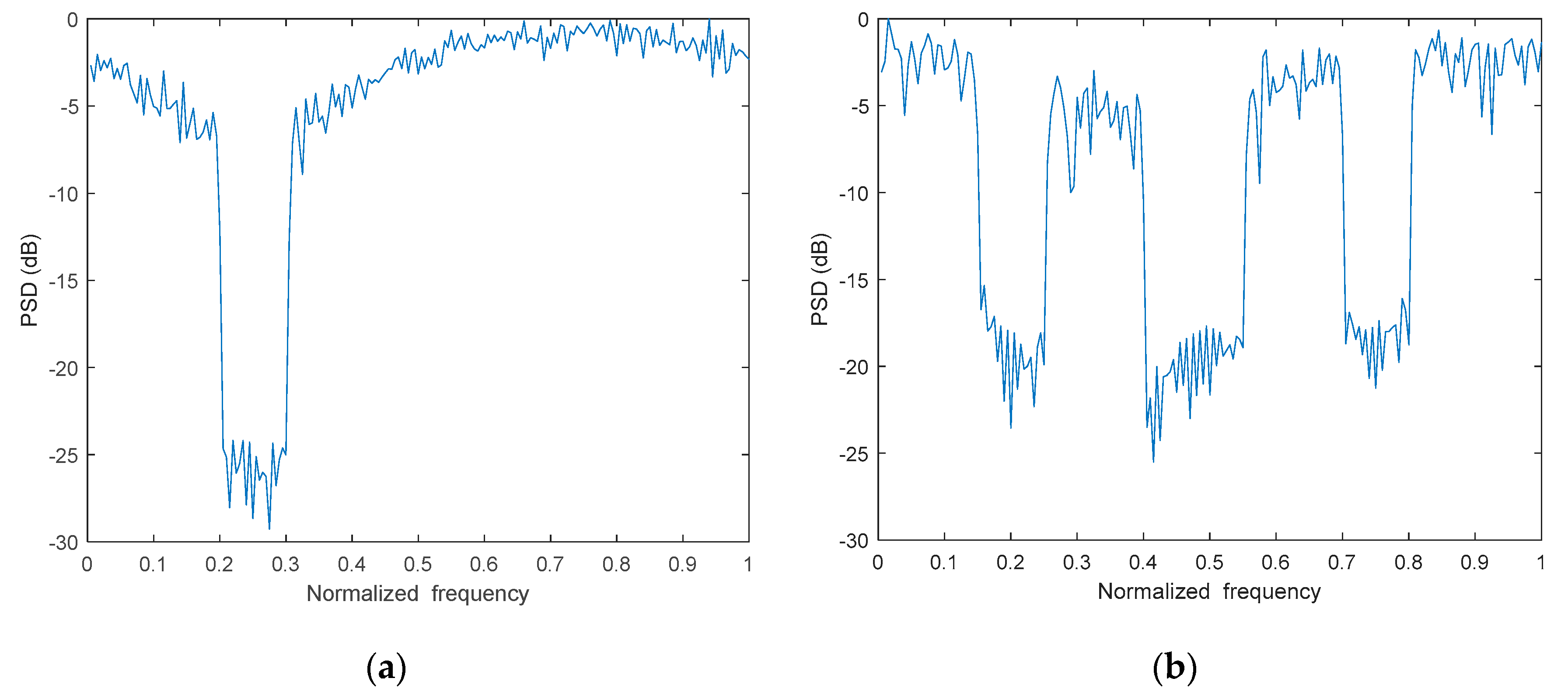
5.2. The Number of Frequency Stopbands

The power spectrum density of the optimized waveform under the different number of frequency stopbands is shown in Figure 10. The frequency stopband of Figure 10a is [0.2, 0.3), the frequency stopband of Figure 10b is [0.15, 0.25) U [0.4, 0.55) U [0.7, 0.8), the frequency stopband of Figure 10c is [0.2, 0.35) U [0.42, 0.5) U [0.65, 0.72) U [0.8, 0.87) U [0.9, 0.95), and the frequency stopband of Figure 10d is [0.08, 0.16) U [0.25, 0.3) U [0.35, 0.4) U [0.45, 0.55) U [0.6, 0.7) U [0.78, 0.85) U [0.9, 0.95).

It can be seen from the figure that, when there is only one frequency stopband, the waveform PSD notch depth is the lowest, which is −25 dB. With the increase in the number of stopbands, the notch depth of each frequency stopband becomes shallow, which will cause performance degradation of interference suppression. Therefore, in the process of waveform design, it is necessary to set the number of stopbands reasonably.

5.3. Frequency Stopband Weighting Effect

In practice, the interference intensity of each interference frequency band received by airborne radar is not the same. If the notch of the same depth is formed, the frequency band with stronger interference intensity will not be effectively suppressed, and the weaker frequency band will occupy more resources. Therefore, the frequency stopband resources can be reasonably allocated by changing the weight vector of the SMIA algorithm Equation (6). This section assumes that the sequence length is N = 100, the region of reducing the sidelobes of specified-range cells is $k\in (3,100)$, the weighting factor $\lambda =0.9$, the frequency band with strong interference intensity is [0.4, 0.55], and the frequency band with weak interference intensity is [0.15, 0.25) U [0.7, 0.8). The frequency stopbands [0.15, 0.25) U [0.4, 0.55) U [0.7, 0.8) in Figure 11a are evenly weighted, namely, the weight vector is set to 1, the frequency stopband [0.15, 0.25) U [0.7, 0.8) weight vector in Figure 11b is set to 0.2, and [0.4, 0.55) is set to 1. The notch depths of the three frequency stopbands are basically the same when uniform weighting is set, and they are all about −18 dB. When the weight vector of [0.15, 0.25) U [0.7, 0.8) is changed to 0.2, the frequency stopbands on both sides increase significantly, and the intermediate-frequency stopband decreases. At this time, the interference is effectively suppressed, and the spectrum stopband resources are also effectively utilized.

5.4. WISL and Merit Factor

The weighted integral sidelobe level is one of the criteria for measuring the quality of the sequence, which is defined as

$$WISL=2{\displaystyle \sum _{k=1}^{N-1}{w}_k{\left|r_k\right|}^2}\begin{array}{c}\end{array}\left(w_k\ge 0\right)$$

(36)

where the smaller the WISL value, the better the final sequence obtained by the optimization algorithm.

Minimizing the WISL is equivalent to maximizing the merit factor (MF), which is defined as

$$M\mathbf{F}=\frac{{\left|r_0\right|}^2}{WISL}$$

(37)

The variation of the merit factor and normalized WISL value with the number of iterations under the constant modulus constraint and PAR constraint of different algorithms are shown in Figure 12 and Figure 13, respectively. Here, the CAN algorithm in [26], the WeSCAN algorithm in [27], the SMIA-ISL algorithm in this paper under ISL criteria, and the SMIA-WISL algorithm in this paper under WISL criteria are mainly compared.

From Figure 12a, it can be found that the normalized WISL values of all algorithms showed a decreasing trend as the number of iterations increased. The curves tended to be horizontal and eventually converge as the number of iterations increased. The convergence rate of the SMIA algorithm was the fastest either under the ISL criterion or the WISL criterion. The curve tended to be horizontal at about 90 iterations, and its normalized WISL value eventually converged at −24.59 dB and −25.10 dB. Because the WeSCAN algorithm requires a large number of matrix operations and has high computational complexity, its convergence speed is slower than the SMIA algorithm, but it can finally obtain a smaller WISL value, so the WeSCAN algorithm is inferior to the SMIA algorithm but better than the CAN algorithm. Since the merit factor of Figure 12b is actually the reciprocal of the WISL value, the conclusion is basically consistent with Figure 12a, and the merit factor of the SMIA algorithm is the largest.

As shown in Figure 13a,b, the WISL value and merit factor of each algorithm under the PAR constraint are basically consistent with the constant modulus constraint, but the numerical value is much higher than the constant modulus constraint. This is because the PAR constraint relaxes the peak average ratio and increases the degree of freedom of waveform design, so a smaller WISL value and greater merit factor are obtained.

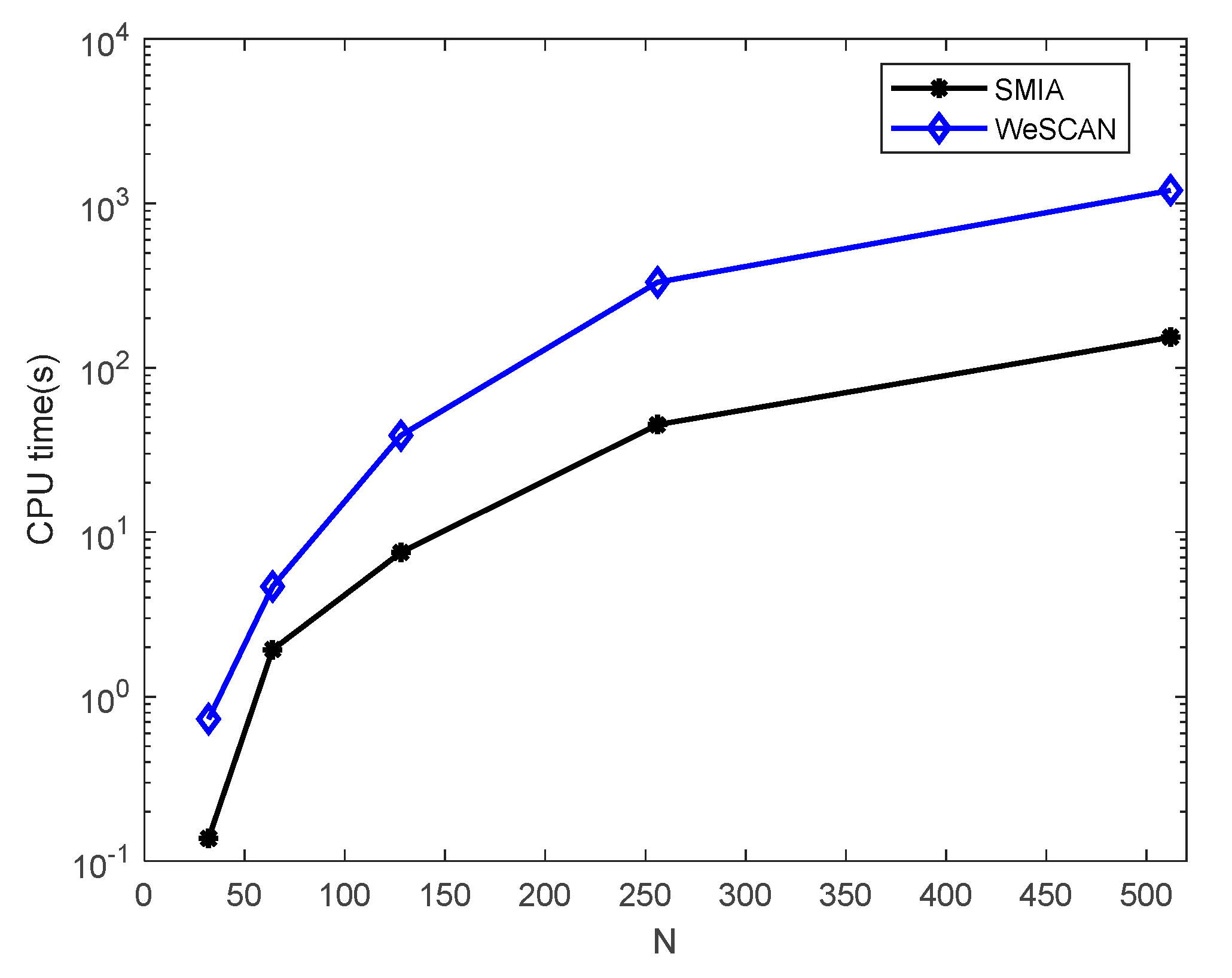
5.5. The Amount of Computation

The running time of the WeSCAN algorithm and SMIA algorithm was compared by a simulation shown in Figure 14. The simulation environment was MATLAB 2022a/Windows 10, Intel Core i7-8750H CPU@2.2 GHz. In this experiment, the region of reducing the sidelobes of specified-range cells was $k\in (3,100)$, the frequency stopband was [0.15, 0.25) U [0.4, 0.55) U [0.7, 0.8), and the weighting factor $\lambda =0.9$. Due to the introduction of a large number of DFT operations and eigenvalue decomposition in each iteration of the WeSCAN algorithm, the time complexity increased rapidly with the increase in N; the SMIA algorithm only involves the FFT operation and has low time complexity.

6. Conclusions

In this paper, an algorithm for designing sparse-frequency waveforms for airborne early warning radar based on the minimum wave energy in a stopband was proposed to solve the practical problem of dense interference encountered by the low-frequency-band airborne early warning radar working over land. Theoretical analysis and simulation experiments showed that the cognitive waveform optimization design algorithm proposed in this paper can effectively suppress dense interference and reduce the influence of strongly isolated point clutter and interference. It can also form low-range sidelobes at specified-range cells, which is beneficial for dim target detection. In addition, the waveform optimized by the algorithm in this paper has good low-intercept performance, and because the waveform is optimized by the circular iterative algorithm based on FFT operation, it has low computational complexity and is convenient for engineering implementation.

In practical engineering, the main lobe interference and side lobe interference exist simultaneously in complex electromagnetic environments; in the process of the optimization design of the transmitted waveform, the influence of main-lobe interference should be emphasized. At the same time, the bandwidth of the sparse waveform determines the clutter intensity of the airborne radar receiver. The parameters such as the stopband position and the number of stopbands can be obtained by detecting the spatial interference distribution in passive mode. The bandwidth of the transmitted waveform to some extent determines the clutter-to-noise ratio (CNR) of the airborne radar receiver, and its size is determined by the clutter suppression ability of the airborne radar system.

References

1. Nunn, C.; Moyer, L.R. Spectrally-compliant waveforms for wideband radar. IEEE Aerosp. Electron. Syst. Mag. 2012, 27, 11–15. [Google Scholar] [CrossRef]
2. Haykin, S. Cognitive radar: A way of the future. IEEE Signal Process. Mag. 2006, 23, 30–40. [Google Scholar] [CrossRef]
3. Guerci, J.R. Cognitive Radar: A Knowledge-Aided Fully Adaptive Approach. In Proceedings of the IEEE Radar Conference 2010, Arlington, VA, USA, 10–14 May 2010; pp. 1365–1370. [Google Scholar]
4. Haykin, S.; Xue, Y.; Davidson, T.N. Cognitive Radar: Optimal waveform design for cognitive radar. In Proceedings of the 42nd Asilomar Conference on Signals, Systems and Computers, Pacific Grove, CA, USA, 26–29 October 2008; pp. 3–7. [Google Scholar]
5. Haykin, S. New generation of radar systems enabled with cognition. In Proceedings of the IEEE Radar Conference 2010, Arlington, VA, USA, 10–14 May 2010. [Google Scholar]
6. Mitola, J. Software radios: Survey, critical evaluation and future directions. IEEE Aerosp. Electron. Syst. Mag. 1993, 8, 25–36. [Google Scholar] [CrossRef] [PubMed]
7. Haykin, S.; Xue, Y.; Setoodeh, P. Cognitive radar:step toward bridging the gap between neuroscience and engineering. Proc. IEEE 2012, 100, 3102–3130. [Google Scholar] [CrossRef]
8. Guerci, J.R.; Guerci, R.M.; Ranagaswamy, M.; Bergin, J.S.; Wicks, M.C. CoFAR: Cognitive fully adaptive radar. In Proceedings of the IEEE Radar Conference 2014, Cincinnati, OH, USA, 19–23 May 2014; pp. 984–989. [Google Scholar]
9. Bell, K.L.; Baker, C.J.; Smith, G.E.; Johnson, J.T.; Rangaswamy, M. Cognitive radar framework for target detection and tracking. IEEE J. Sel. Top. Signal Process. 2015, 9, 1427–1439. [Google Scholar] [CrossRef]
10. Guerci, J.R. Cognitive radar:the knowledge-aided fully a daptive approach. Aeronaut. J. 2011, 115, 390–396. [Google Scholar]
11. Smith, G.E.; Cammenga, Z.; Mitchell, A.; Bell, K.L.; Johnson, J.; Rangaswamy, M.; Baker, C. Experiments with cognitive radar. IEEE Aerosp. Electron. Syst. Mag. 2016, 31, 34–46. [Google Scholar] [CrossRef]
12. Huleihel, W.; Tabrikian, J.; Shavit, R. Optimal adaptive waveform design for cognitive MIMO radar. IEEE Trans. Signal Process. 2013, 61, 5075–5089. [Google Scholar] [CrossRef]
13. Jiu, B.; Liu, H.; Zhang, L.; Wang, Y.; Luo, T. Wideband cognitive radar waveform optimization for joint target radar signature estimation and target detection. IEEE Trans. Aerosp. Electron. Syst. 2015, 51, 1530–1546. [Google Scholar] [CrossRef]
14. Feng, X.; Zhao, Z.; Li, F.; Cui, W.; Zhao, Y. Radar phase-coded waveform design with local low range sidelobes based on particle swarm-assisted projection optimization. Remote Sens. 2022, 14, 4186. [Google Scholar] [CrossRef]
15. Savci, K.; Galati, G.; Pavan, G. Low-PAPR waveforms with shaped spectrum for enhanced low probability of intercept noise radars. Remote Sens. 2021, 13, 2372. [Google Scholar] [CrossRef]
16. Mohammad, M.A.B.; Cui, G.; Yu, X.; Fakirah, M.; Elhag, N.A.A. Integrated OFDM waveform design for RadCom system-based signal-to-clutter noise ratio maximization. Remote Sens. 2023, 15, 3554. [Google Scholar] [CrossRef]
17. Zhao, Y.; Zhao, Z.; Tong, F.; Sun, P.; Feng, X.; Zhao, Z. Joint design of transmitting waveform and receiving filter via novel riemannian idea for DFRC System. Remote Sens. 2023, 15, 3548. [Google Scholar] [CrossRef]
18. Zhang, X.; Wang, X.; So, H.C.; Zoubir, A.M.; Cui, G. Min-max optimization for MIMO Radar waveform design with improved power efficiency. IEEE Trans. Signal Process. 2022, 70, 6112–6127. [Google Scholar] [CrossRef]
19. Zheng, Z.; Zhang, Y.; Peng, X.; Xie, H.; Chen, J.; Mo, J.; Sui, Y. MIMO radar waveform design for multipath exploitation using deep learning. Remote Sens. 2023, 15, 2747. [Google Scholar] [CrossRef]
20. Stoica, P.; He, H.; Li, J. Optimization of the receive filter and transmit sequence for active sensing. IEEE Trans. Signal Process. 2012, 60, 1730–1740. [Google Scholar] [CrossRef]
21. Bell, M.R. Information theory and radar waveform design. IEEE Trans. Inf. Theory 1993, 39, 1578–1597. [Google Scholar] [CrossRef]
22. Xu, G.; Zhang, B.; Yu, H.; Chen, J.; Xing, M.; Hong, W. Sparse Synthetic Aperture Radar Imaging from Compressed Sensing and Machine Learning: Theories, Applications and Trends. IEEE Geosci. Remote Sens. Mag. 2022, 10, 32–69. [Google Scholar] [CrossRef]
23. Xu, G.; Xia, X.-G.; Hong, W. Nonambiguous SAR Image Formation of Maritime Targets Using Weighted Sparse Approach. IEEE Trans. Geosci. Remote Sens. 2018, 56, 1454–1465. [Google Scholar] [CrossRef]
24. Kang, M.-S.; Baek, J.-M. Efficient SAR Imaging Integrated With Autofocus via Compressive Sensing. IEEE Geosci. Remote Sens. Lett. 2022, 19, 4514905. [Google Scholar] [CrossRef]
25. Xu, Z.; Zhang, B.; Zhang, Z.; Wang, M.; Wu, Y. Nonconvex-Nonlocal Total Variation Regularization-Based Joint Feature-Enhanced Sparse SAR Imaging. IEEE Geosci. Remote Sens. Lett. 2022, 19, 4515705. [Google Scholar] [CrossRef]
26. Bi, H.; Lu, X.; Yin, Y.; Yang, W.; Zhu, D. Sparse SAR Imaging Based on Periodic Block Sampling Data. IEEE Trans. Geosci. Remote Sens. 2022, 60, 5213812. [Google Scholar] [CrossRef]
27. Kang, M.-S.; Baek, J.-M. SAR Image Reconstruction via Incremental Imaging With Compressive Sensing. IEEE Trans. Aerosp. Electron. Syst. 2023, 59, 4450–4463. [Google Scholar] [CrossRef]
28. Lindenfeld, M.J. Sparse frequency transmit and receive waveform design. IEEE Trans. Aerosp. Electron. Syst. 2004, 40, 851–860. [Google Scholar] [CrossRef]
29. Liu, W.X.; Lesturgie, M.; Lu, Y.L. Real-time sparse frequency design for HFSWR system. IET Electron. Lett. 2007, 43, 1387–1389. [Google Scholar] [CrossRef]
30. Wang, G.H.; Lu, Y.L. Sparse frequency transmit waveform design with soft power constraint by using PSO algorithm. In Proceedings of the IEEE Radar Conference 2008, Roma, Italy, 26–30 May 2008. [Google Scholar]
31. Wang, G.; Lu, Y. Designing single/multiple sparse frequency waveforms with sidelobe constraint. IET Radar Sonar Navig. 2011, 5, 32–38. [Google Scholar] [CrossRef]
32. Liu, W.; Liu, J.; Liu, T.; Chen, H.; Wang, Y.L. Detector Design and Performance Analysis for Target Detection in Subspace Interference. IEEE Signal Process. Lett. 2023, 30, 618–622. [Google Scholar] [CrossRef]
33. Stoica, P.; He, H.; Li, J. New algorithms for designing unimodular sequences with good correlation properties. IEEE Trans. Signal Process. 2009, 57, 1415–1425. [Google Scholar] [CrossRef]
34. He, H.; Stoica, P.; Li, J. Waveform design with stopband and correlation constraints for cognitive radar. In Proceedings of the 2nd International Workshop on Cognitive Information Processing, Elba Island, Italy, 14–16 June 2010; pp. 344–349. [Google Scholar]
35. Wu, H.; Song, Z.; Fan, H.; Li, Y.; Fu, Q. A new algorithm for sparse frequency waveform design with range sidelobes constraint. Chin. J. Electron. 2015, 24, 604–610. [Google Scholar] [CrossRef]
36. Nathan, A.G.; Phaneendra, R.V.; Mark, A.N. Adaptive waveform design and sequential hypothesis testing for target recognition with active sensors. IEEE J. Sel. Top. Signal Process. 2007, 1, 105–113. [Google Scholar]
37. Wu, H.; Song, Z.; Fan, H.; Fu, Q. Designing sequence with low sidelobe levels at specified intervals based on PSD fitting. Electron. Lett. 2015, 51, 99–101. [Google Scholar] [CrossRef]
38. Patton, L.K.; Rigling, B.D. Modulus constraints in adaptive radar waveform design. In Proceedings of the IEEE Radar Conference 2008, Roma, Italy, 26–30 May 2008; pp. 1–6. [Google Scholar]
39. Tropp, J.; Dhillon, I.; Heath, R.; Strohmer, T. Designing structured tight frames via an alternating projection method. IEEE Trans. Inf. Theory 2005, 51, 188–209. [Google Scholar] [CrossRef]
Figure 1. Autocorrelation function and power spectrum density of the proposed SMIA algorithm ( λ 0.9 ,   k ( 3 , 50 ) ). (a) Autocorrelation function; (b) power spectrum density.
Remotesensing 15 04322 g001
Figure 2. Autocorrelation function and power spectrum density of the WeSCAN algorithm ( λ = 0.9 , k ( 3 , 50 ) ). (a) Autocorrelation function; (b) power spectrum density.
Remotesensing 15 04322 g002
Figure 3. Autocorrelation function and power spectrum density of the proposed SMIA algorithm (PAR ≤ 2). (a) Autocorrelation function; (b) power spectrum density.
Remotesensing 15 04322 g003
Figure 4. Autocorrelation function and power spectrum density of the WeSCAN algorithm (PAR ≤ 2). (a) Autocorrelation function; (b) power spectrum density.
Remotesensing 15 04322 g004
Figure 5. Signal waveform and matched filtering output when the frequency stopband is inconsistent with the interference band. (a) The transmitted waveform PSD; (b) the interference waveform PSD; (c) the echo waveform PSD; (d) matched filtering output.
Remotesensing 15 04322 g005
Figure 6. Signal waveform and matched filtering output when the interference frequency band falls within the frequency stopband. (a) The transmitted waveform PSD; (b) the interference waveform PSD; (c) the echo waveform PSD; (d) matched filtering output.
Remotesensing 15 04322 g006aRemotesensing 15 04322 g006b
Figure 7. The time–frequency distribution of the optimized waveform.
Remotesensing 15 04322 g007
Figure 8. Performance comparison between sparse-frequency waveform and non-sparse-frequency waveform. (a) Autocorrelation function; (b) autocorrelation function (partial).
Remotesensing 15 04322 g008
Figure 9. Graph of P corr and P stop changing with λ .
Remotesensing 15 04322 g009
Figure 10. Optimization results under the different number of frequency stopbands. (a) One stopband; (b) three stopbands; (c) five stopbands; (d) seven stopbands.
Remotesensing 15 04322 g010aRemotesensing 15 04322 g010b
Figure 11. Optimization results under different weightings of the frequency stopband. (a) Uniform weighting; (b) non-uniform weighting.
Remotesensing 15 04322 g011
Figure 12. Normalized WISL and merit factor of different algorithms (constant modulus constraint). (a) Normalized WISL; (b) merit factor.
Remotesensing 15 04322 g012
Figure 13. Normalized WISL and merit factor of different algorithms (PAR ≤ 2). (a) Normalized WISL; (b) merit factor.
Remotesensing 15 04322 g013
Figure 14. The comparison of the running time.
Remotesensing 15 04322 g014
Disclaimer/Publisher’s Note: The statements, opinions and data contained in all publications are solely those of the individual author(s) and contributor(s) and not of MDPI and/or the editor(s). MDPI and/or the editor(s) disclaim responsibility for any injury to people or property resulting from any ideas, methods, instructions or products referred to in the content.