Author Contributions
Conceptualization, Q.W., Z.Z. and T.S.; methodology, Q.W. and Z.Z.; software, Z.Z.; validation, Z.Z.; formal analysis, Z.Z., X.C. and J.S.; resources, Q.W., J.S. and T.S.; data curation, Z.Z. and X.C.; writing—original draft preparation, Z.Z.; writing—review and editing, Q.W. and J.S.; visualization, Z.Z.; supervision, T.S.; project administration, Z.W.; funding acquisition, Z.W., Q.W., and T.S. All authors have read and agreed to the published version of the manuscript.
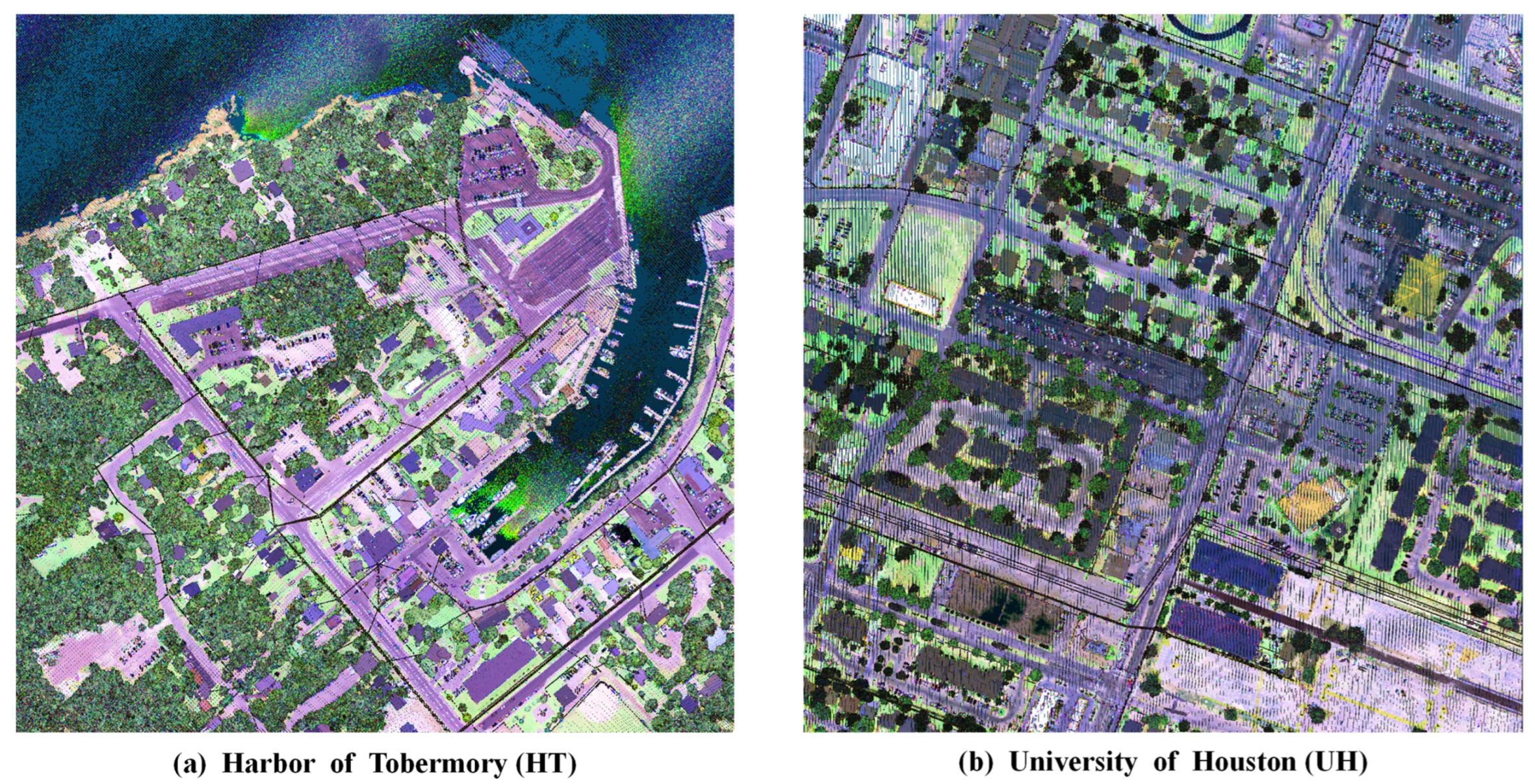
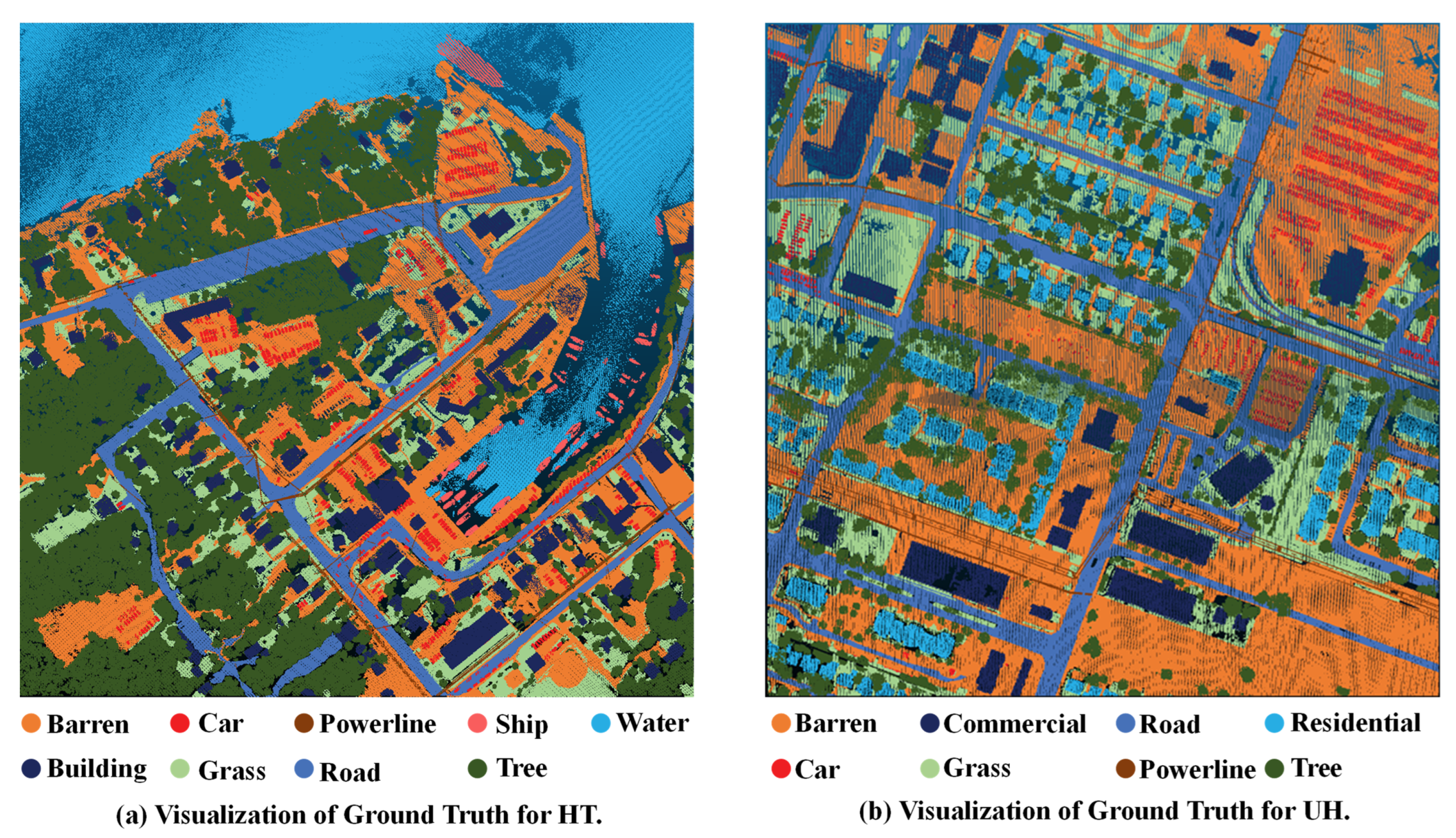
Figure 1.
Visualization of two scenes of multispectral point cloud datasets: (a) Harbor of Tobermory (HT) and (b) University of Houston (UH).
Figure 1.
Visualization of two scenes of multispectral point cloud datasets: (a) Harbor of Tobermory (HT) and (b) University of Houston (UH).
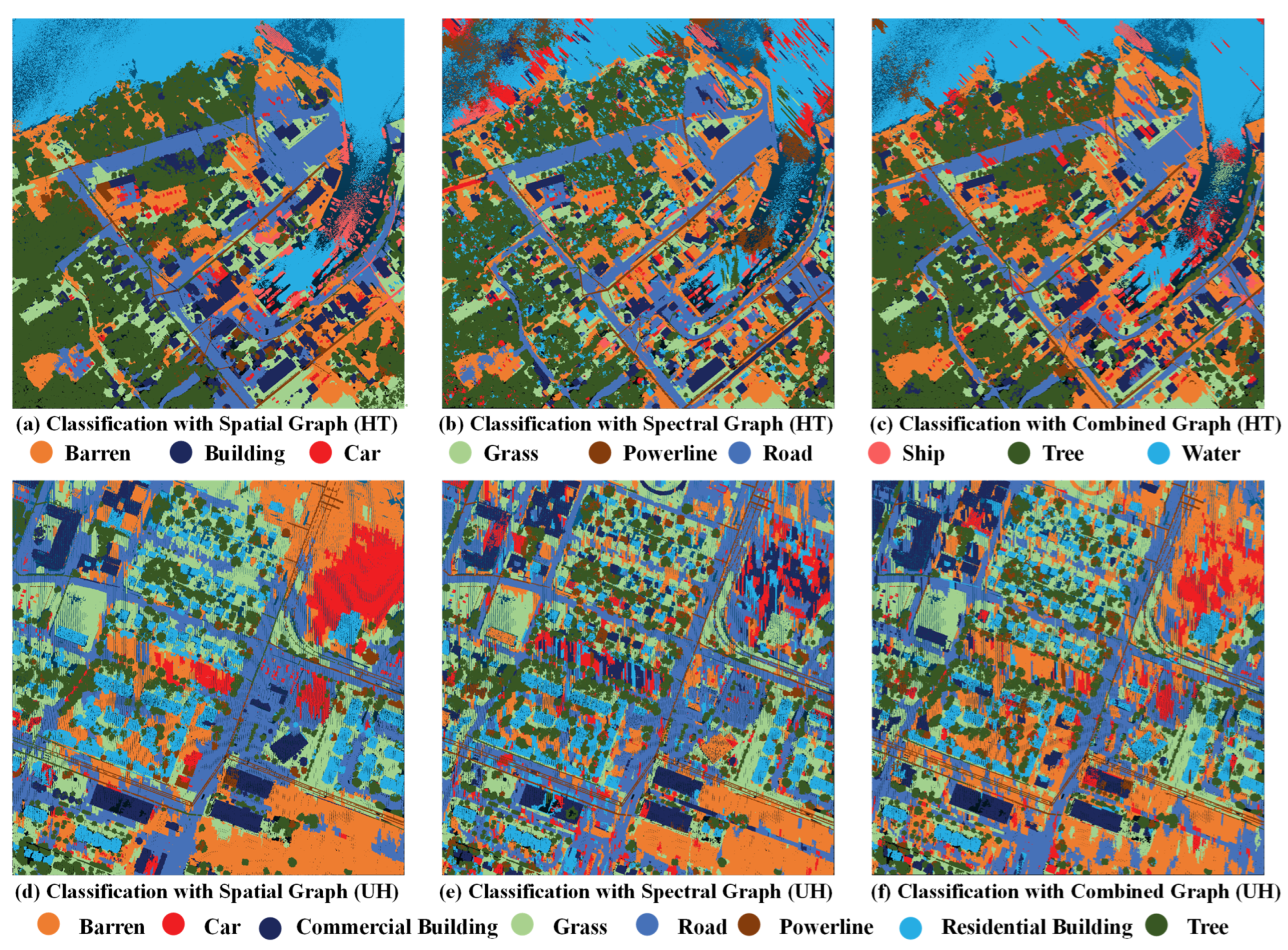
Figure 2.
Visualization of differences between three technical routes for constructing graphs from two datasets: (a) classification with a spatial graph for the HT dataset; (b) classification with a spectral graph for the HT dataset; (c) classification with a combined graph on the HT dataset; (d) classification with a spatial graph for the UH dataset. (e) classification with a spectral graph for the UH dataset. (f) classification with a combined graph for the UH dataset.
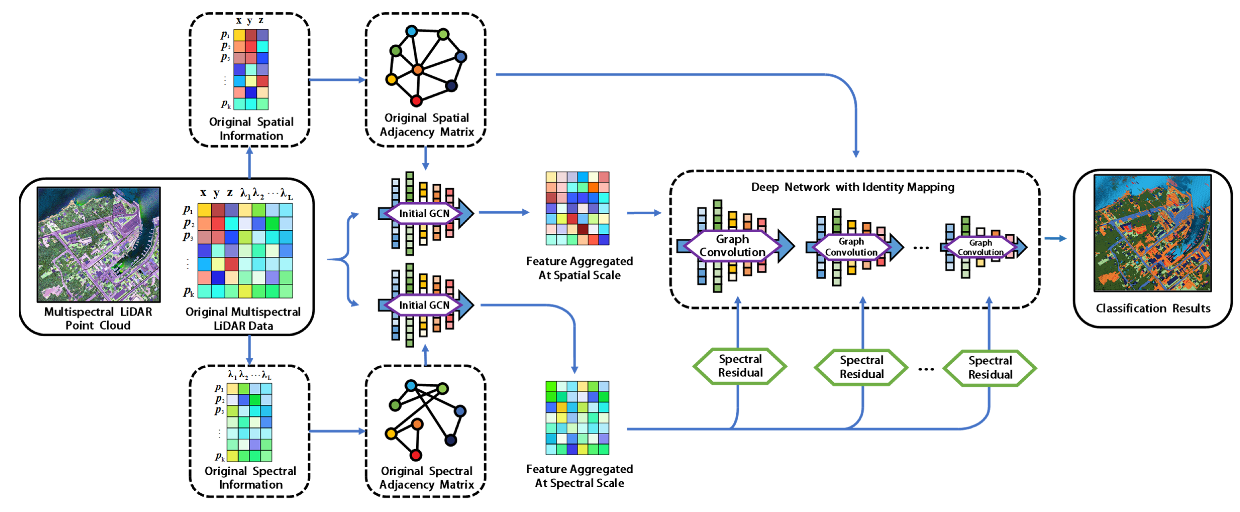
Figure 3.
Overall structure of the proposed DSGCN-ASR.
Figure 3.
Overall structure of the proposed DSGCN-ASR.
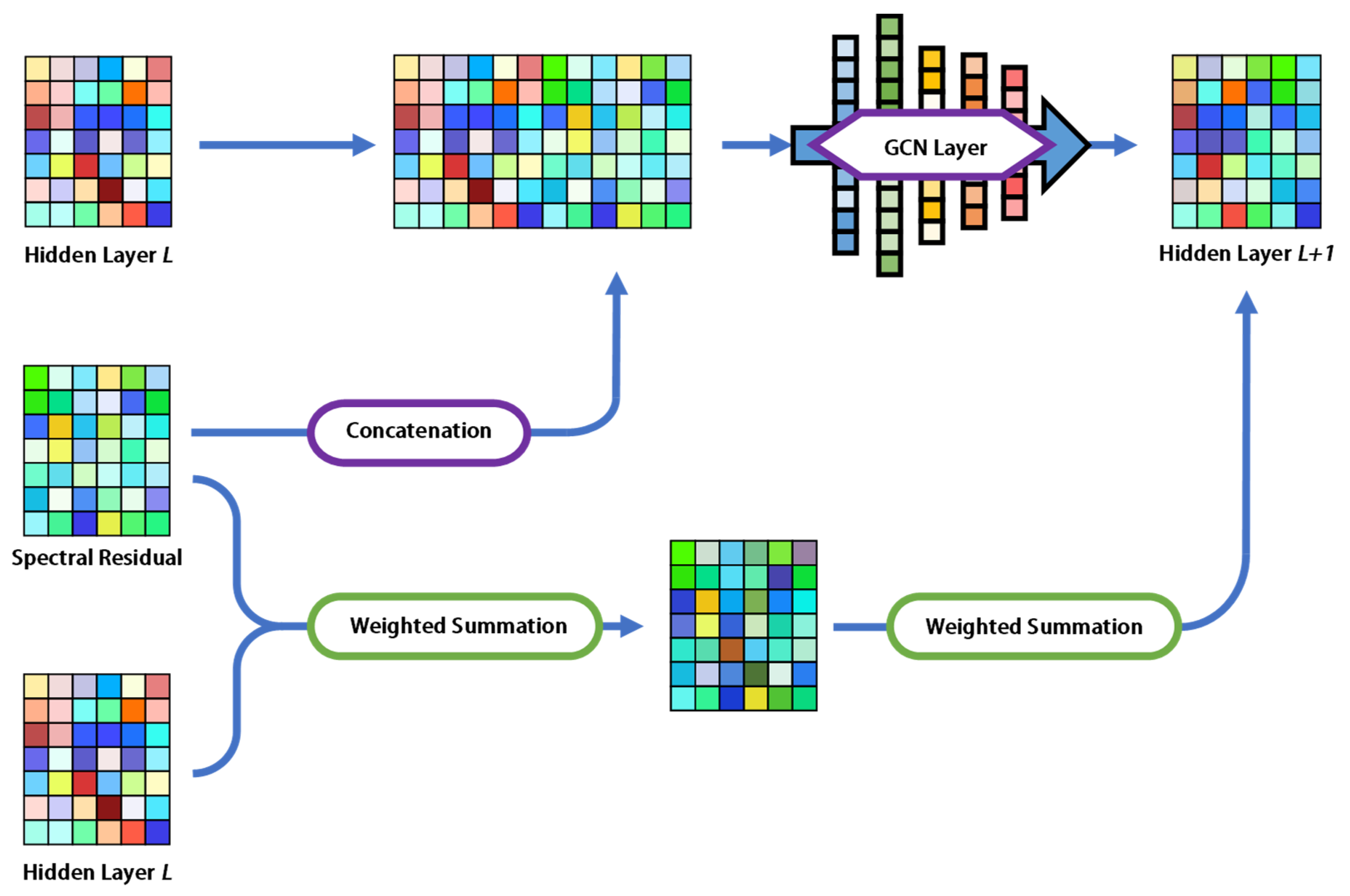
Figure 4.
Combining patterns of adaptive spectral residuals in each layer.
Figure 4.
Combining patterns of adaptive spectral residuals in each layer.
Figure 5.
Visualization of ground truth for two datasets: (a) HT; (b) UH.
Figure 5.
Visualization of ground truth for two datasets: (a) HT; (b) UH.
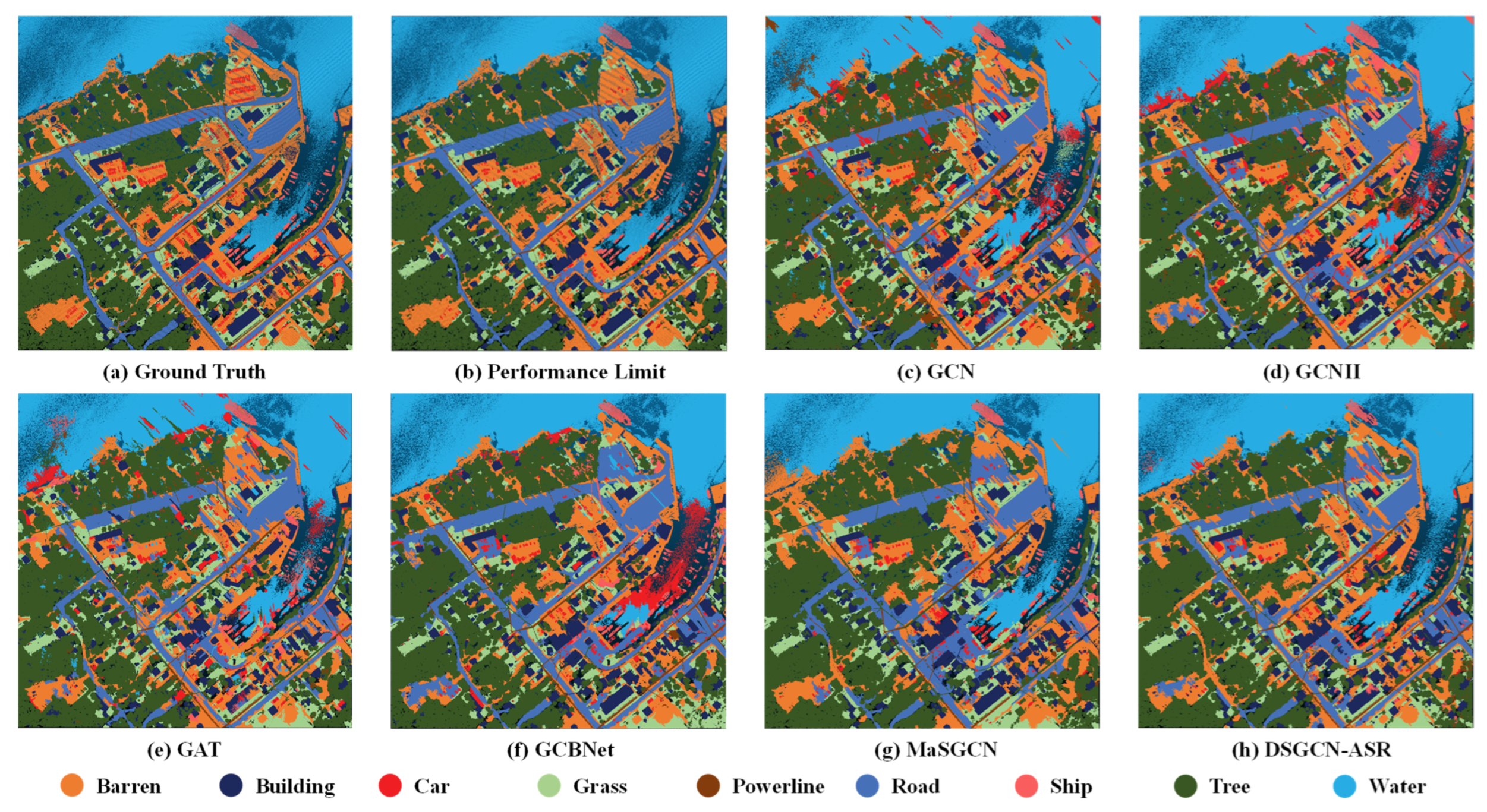
Figure 6.
Visualization of classification results on HT dataset. (a) Visualization of the ground truth; (b) performance limit due to superpoint segmentation; visualization of classification results of (c) GCN, (d) GCNII, (e) GAT, (f) GCBNet, (g) MaSGCN, and (h) DSGCN-ASR (ours).
Figure 6.
Visualization of classification results on HT dataset. (a) Visualization of the ground truth; (b) performance limit due to superpoint segmentation; visualization of classification results of (c) GCN, (d) GCNII, (e) GAT, (f) GCBNet, (g) MaSGCN, and (h) DSGCN-ASR (ours).
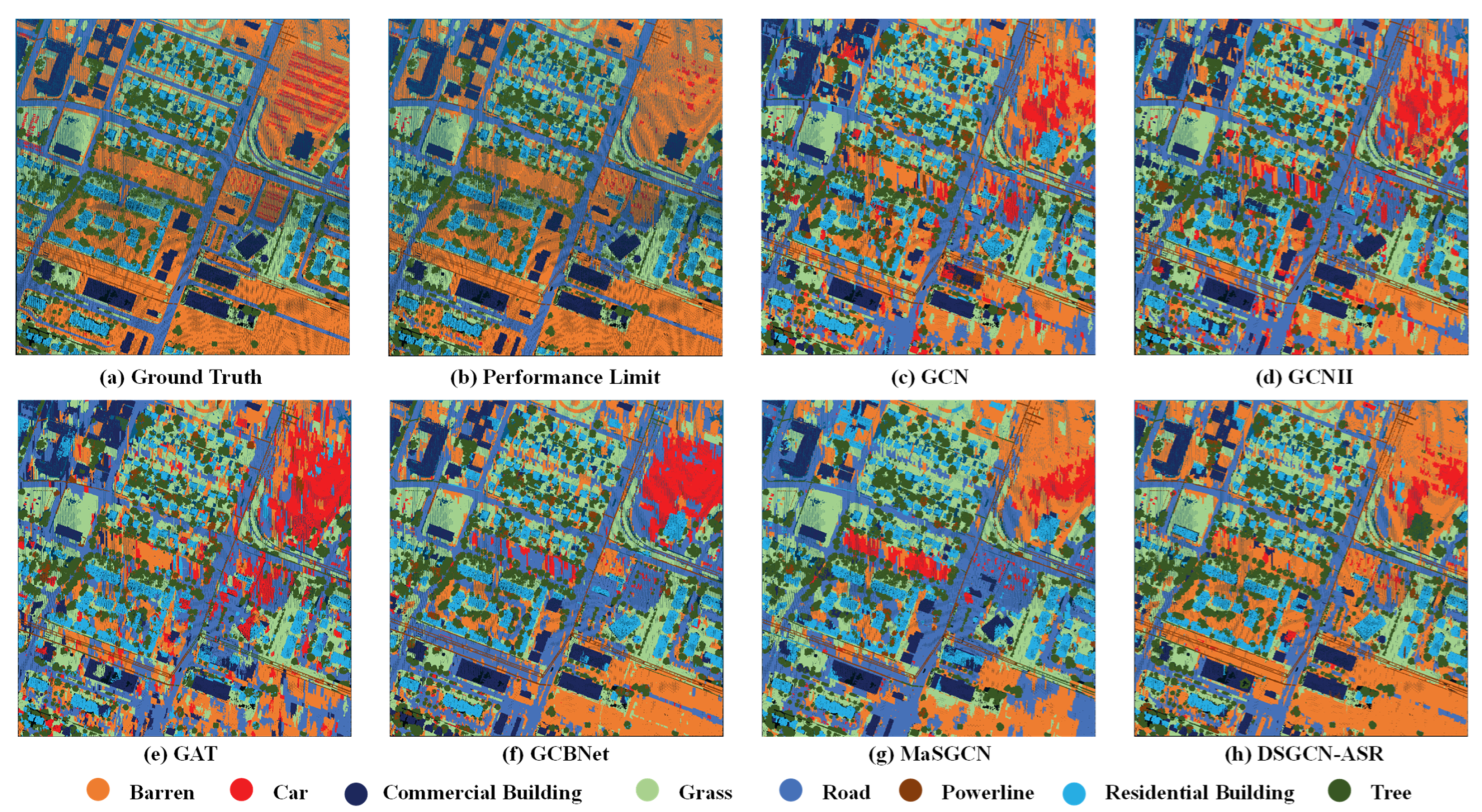
Figure 7.
Visualization of classification results on the UH dataset: (a) visualization of the ground truth; (b) performance limit due to superpoint segmentation. Visualization of classification results of (c) GCN, (d) GCNII, (e) GAT, (f) GCBNet, (g) MaSGCN, and (h) DSGCN-ASR (ours).
Figure 7.
Visualization of classification results on the UH dataset: (a) visualization of the ground truth; (b) performance limit due to superpoint segmentation. Visualization of classification results of (c) GCN, (d) GCNII, (e) GAT, (f) GCBNet, (g) MaSGCN, and (h) DSGCN-ASR (ours).
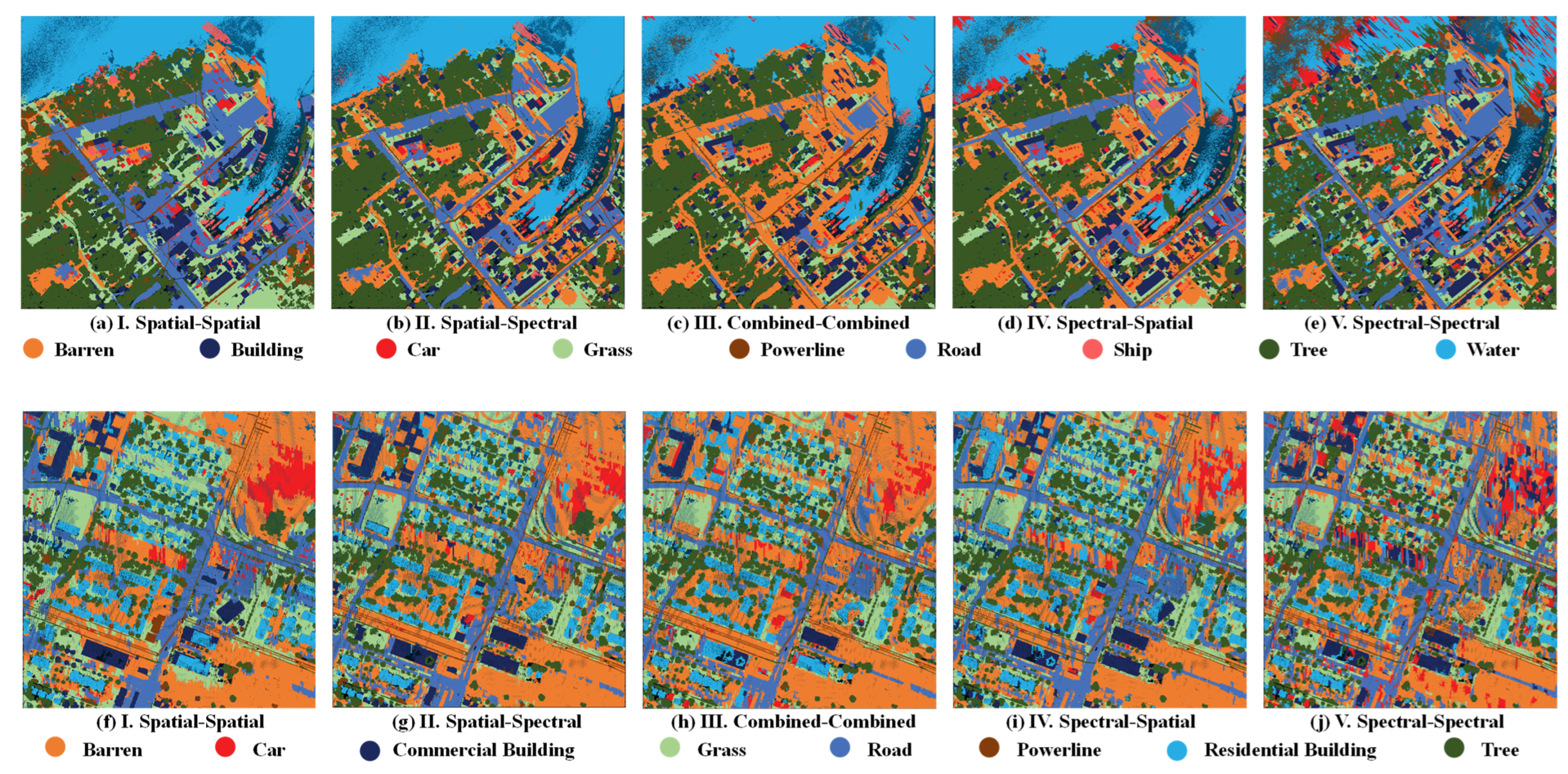
Figure 8.
Visualization of ablation results: (a) group I, (b) group II, (c) group III, (d) group IV, and (e) group V on the HT dataset; (f) group I, (g) group II, (h) group III, (i) group IV, and (j) group V on the UH dataset.
Figure 8.
Visualization of ablation results: (a) group I, (b) group II, (c) group III, (d) group IV, and (e) group V on the HT dataset; (f) group I, (g) group II, (h) group III, (i) group IV, and (j) group V on the UH dataset.
Figure 9.
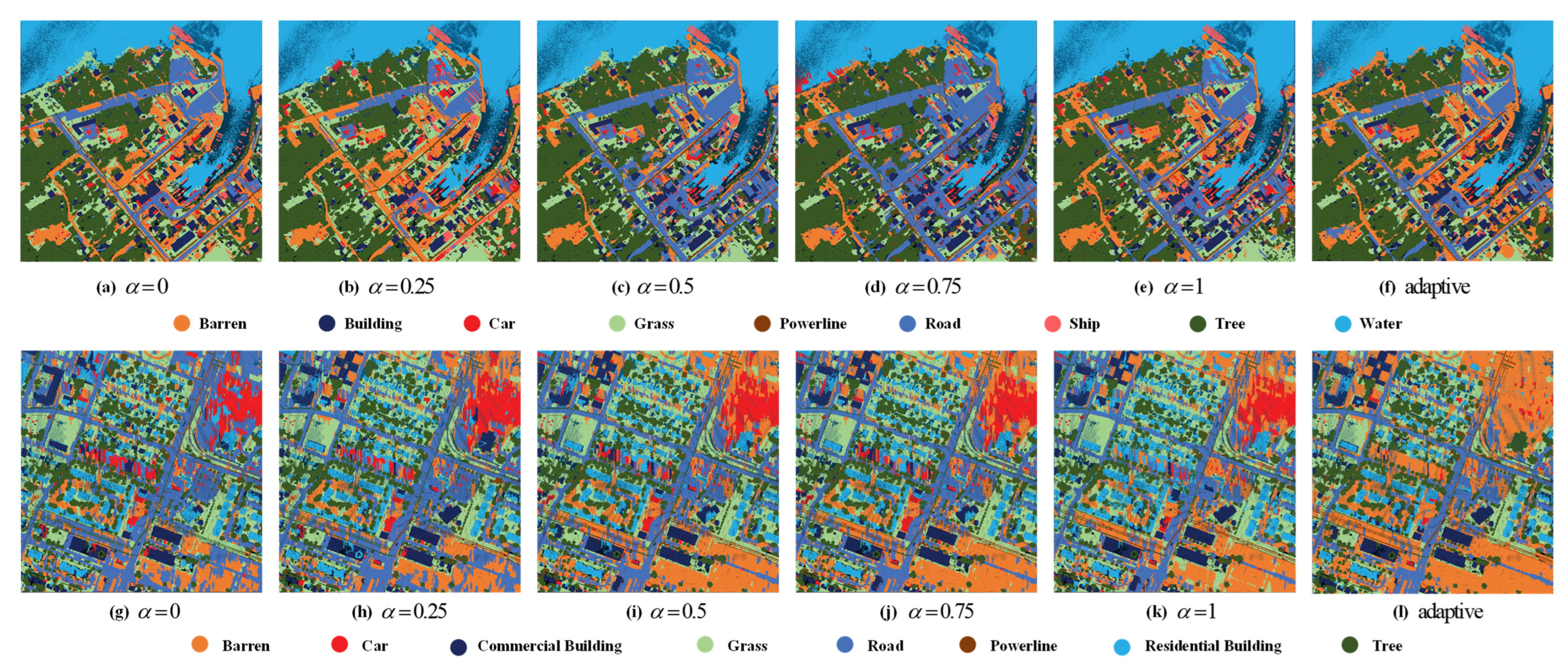
Visualization of the parametric analysis experiment for when set to (a) 0, (b) 0.25, (c) 0.5, (d) 0.75, (e) 1, and (f) an adaptive value on the HT dataset and (g) 0, (h) 0.25, (i) 0.5, (j) 0.75, (k) 1, and (l) an adaptive value on the UH dataset.
Figure 9.
Visualization of the parametric analysis experiment for when set to (a) 0, (b) 0.25, (c) 0.5, (d) 0.75, (e) 1, and (f) an adaptive value on the HT dataset and (g) 0, (h) 0.25, (i) 0.5, (j) 0.75, (k) 1, and (l) an adaptive value on the UH dataset.
Figure 10.
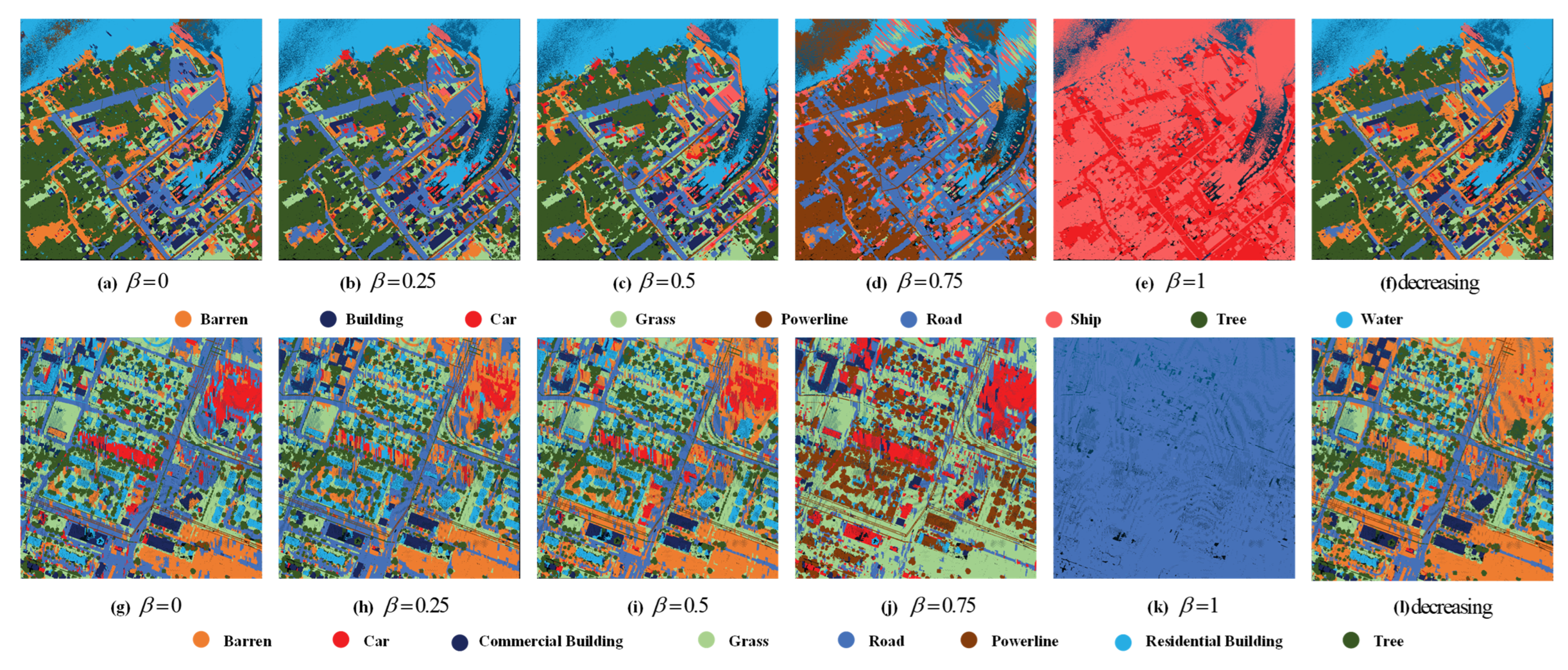
Visualization of the parametric analysis experiment for when set to (a) 0, (b) 0.25, (c) 0.5, (d) 0.75, (e) 1, and (f) a decreasing value on the HT dataset and (g) 0 (h) 0.25, (i) 0.5, (j) 0.75, (k) 1, and (l) a decreasing value on the UH dataset.
Figure 10.
Visualization of the parametric analysis experiment for when set to (a) 0, (b) 0.25, (c) 0.5, (d) 0.75, (e) 1, and (f) a decreasing value on the HT dataset and (g) 0 (h) 0.25, (i) 0.5, (j) 0.75, (k) 1, and (l) a decreasing value on the UH dataset.
Figure 11.
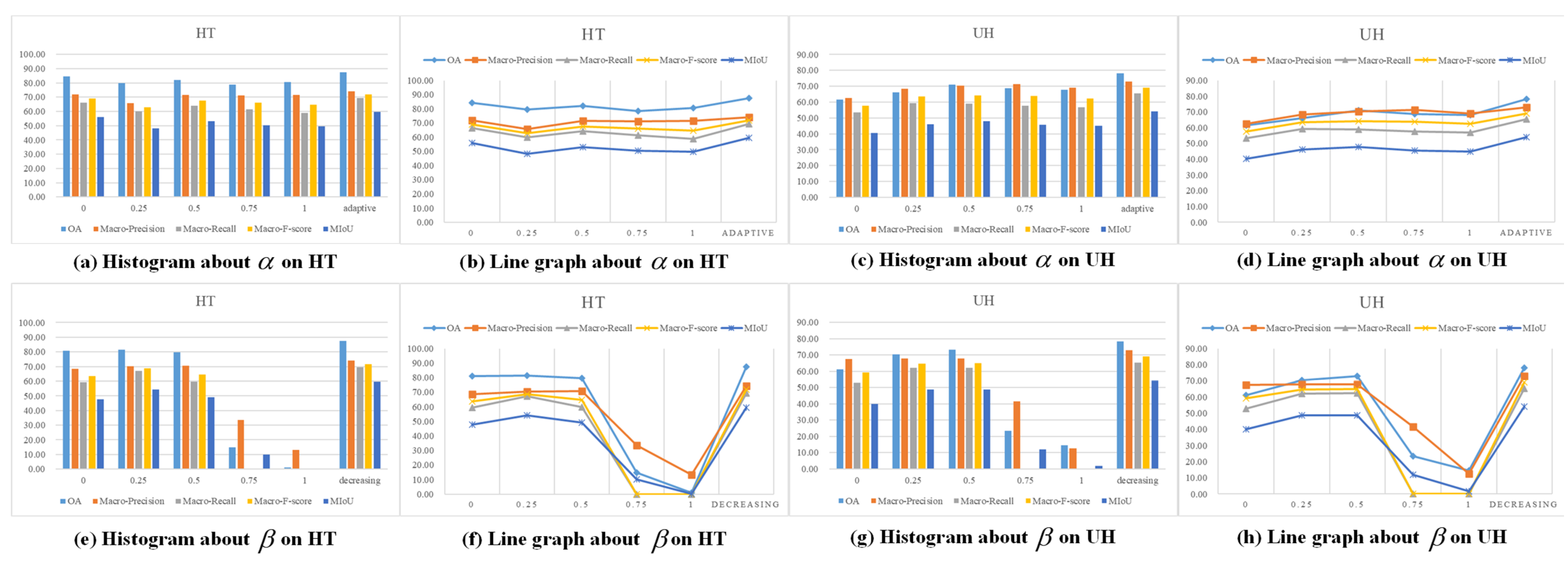
Histograms and line graphs of results of parametric analysis experiment. (a) Histogram of on the HT dataset. (b) Line graph of on the HT dataset. (c) Histogram of on the UH dataset. (d) Line graph of on the UH dataset. (e) Histogram of on the HT dataset. (f) Line graph of on the HT dataset. (g) Histogram of on the UH dataset. (h) Line graph of on the UH dataset.
Figure 11.
Histograms and line graphs of results of parametric analysis experiment. (a) Histogram of on the HT dataset. (b) Line graph of on the HT dataset. (c) Histogram of on the UH dataset. (d) Line graph of on the UH dataset. (e) Histogram of on the HT dataset. (f) Line graph of on the HT dataset. (g) Histogram of on the UH dataset. (h) Line graph of on the UH dataset.
Table 1.
Overall evaluation metrics (%) for classification results on the HT dataset.
Table 1.
Overall evaluation metrics (%) for classification results on the HT dataset.
| Method | GCN [30] | GCNII [33] | GAT [31] | GCBNet [32] | MaSGCN [29] | DSGCN-ASR (Ours) |
|---|
| OA | 81.36 | 84.83 | 84.77 | 84.70 | 82.81 | 87.57 |
| Macro precision | 72.30 | 79.17 | 71.71 | 77.84 | 69.55 | 74.23 |
| Macro recall | 61.32 | 64.68 | 62.04 | 66.58 | 67.71 | 69.45 |
| Macro F score | 66.36 | 71.19 | 66.53 | 71.77 | 68.62 | 71.76 |
| MIoU | 51.84 | 55.96 | 53.08 | 57.36 | 54.94 | 59.51 |
Table 2.
Evaluation metrics (%) for classification results in each class on the HT dataset.
Table 2.
Evaluation metrics (%) for classification results in each class on the HT dataset.
| Method | Class | Barren | Building | Car | Grass | Powerline | Road | Ship | Tree | Water |
|---|
| GCN [30] | Precision | 75.50
| 72.88 | 33.42 | 87.70 | 66.37 | 82.38 | 57.34 | 83.85 | 91.24 |
| Recall | 82.45 | 69.97 | 20.24 | 81.09 | 4.89 | 70.57 | 34.61 | 99.20 | 88.85 |
| F-score | 78.82 | 71.39 | 25.21 | 84.27 | 9.11 | 76.02 | 43.16 | 90.88 | 90.03 |
| IoU | 65.04 | 55.51 | 14.42 | 72.81 | 4.77 | 61.31 | 27.52 | 83.29 | 81.86 |
| GCNII [33] | Precision | 71.42 | 79.15 | 38.97 | 88.60 | 82.17 | 88.57 | 82.58 | 89.35 | 91.71 |
| Recall | 85.88 | 77.71 | 28.40 | 88.44 | 9.12 | 67.80 | 31.06 | 99.40 | 94.29 |
| F-score | 77.99 | 78.42 | 32.86 | 88.52 | 16.42 | 76.80 | 45.14 | 94.11 | 92.98 |
| IoU | 63.92 | 64.50 | 19.66 | 79.41 | 8.94 | 62.34 | 29.15 | 88.87 | 86.89 |
| GAT [31] | Precision | 72.37 | 71.53 | 29.14 | 88.46 | 51.50 | 79.46 | 70.75 | 92.60 | 89.59 |
| Recall | 79.67 | 69.64 | 18.86 | 82.95 | 21.48 | 67.78 | 35.53 | 98.98 | 83.46 |
| F-score | 75.85 | 70.57 | 22.90 | 85.62 | 30.32 | 73.16 | 47.31 | 95.68 | 86.42 |
| IoU | 61.09 | 54.53 | 12.93 | 74.85 | 17.87 | 57.67 | 30.98 | 91.72 | 76.08 |
| GCBNet [32] | Precision | 62.48 | 90.04 | 42.23 | 88.37 | 69.87 | 91.39 | 75.02 | 90.54 | 90.63 |
| Recall | 85.51 | 69.97 | 32.96 | 81.76 | 41.27 | 58.92 | 32.42 | 99.33 | 97.02 |
| F-score | 72.21 | 78.75 | 37.02 | 84.94 | 51.89 | 71.65 | 45.27 | 94.73 | 93.71 |
| IoU | 56.50 | 64.95 | 22.72 | 73.82 | 35.04 | 55.83 | 29.26 | 89.99 | 88.17 |
| MaSGCN [29] | Precision | 59.29 | 81.43 | 40.32 | 71.74 | 41.06 | 73.88 | 67.51 | 94.90 | 95.82 |
| Recall | 71.21 | 73.56 | 57.01 | 67.02 | 33.76 | 55.67 | 56.19 | 97.41 | 97.60 |
| F-score | 64.70 | 77.29 | 47.23 | 69.30 | 37.05 | 63.50 | 61.33 | 96.13 | 96.70 |
| IoU | 47.82 | 62.99 | 30.92 | 53.02 | 22.74 | 46.52 | 44.23 | 92.56 | 93.62 |
| DSGCN-ASR (ours) | Precision | 72.18 | 88.36 | 29.28 | 90.95 | 69.95 | 77.08 | 47.02 | 95.41 | 97.86 |
| Recall | 78.40 | 78.74 | 38.73 | 86.34 | 33.12 | 64.81 | 48.64 | 99.05 | 97.24 |
| F-score | 75.16 | 83.27 | 33.35 | 88.59 | 44.96 | 70.41 | 47.81 | 97.19 | 97.55 |
| IoU | 60.21 | 71.34 | 20.01 | 79.51 | 29.00 | 54.34 | 31.42 | 94.54 | 95.21 |
Table 3.
Overall evaluation metrics (%) for classification results on the UH dataset.
Table 3.
Overall evaluation metrics (%) for classification results on the UH dataset.
| Method | GCN [30] | GCNII [33] | GAT [31] | GCBNet [32] | MaSGCN [29] | DSGCN-ASR (Ours) |
|---|
| OA | 67.39 | 66.80 | 61.31 | 69.47 | 64.53 | 78.20
|
| Macro precision | 67.76 | 72.75 | 66.31 | 75.26 | 68.48 | 73.03 |
| Macro recall | 54.30 | 58.29 | 50.87 | 62.37 | 57.86 | 65.41 |
| Macro F score | 60.29 | 64.72 | 57.57 | 68.21 | 62.72 | 69.01 |
| MIoU | 42.89 | 46.52 | 38.81 | 50.95 | 45.03 | 54.02 |
Table 4.
Evaluation metrics (%) for classification results in each class on the UH dataset.
Table 4.
Evaluation metrics (%) for classification results in each class on the UH dataset.
| Method | Class | Barren | Car | Commercial | Grass | Road | Powerline | Residential | Tree |
|---|
| GCN [30] | Precision | 54.13 | 36.22 | 70.84 | 81.62 | 76.47 | 70.78 | 74.60 | 77.39 |
| Recall | 80.05 | 15.41 | 49.31 | 74.47 | 51.76 | 16.41 | 51.94 | 95.05 |
| F score | 64.59 | 21.63 | 58.14 | 77.88 | 61.73 | 26.64 | 61.24 | 85.32 |
| IoU | 47.70 | 12.12 | 40.99 | 63.77 | 44.65 | 15.37 | 44.13 | 74.39 |
| GCNII [33] | Precision | 44.95 | 45.80 | 81.14
| 84.53 | 85.18 | 81.93 | 77.36 | 81.10 |
| Recall | 83.79 | 13.00 | 59.87 | 73.33 | 49.13 | 22.34 | 68.81 | 96.07 |
| F score | 58.51 | 20.26 | 68.90 | 78.53 | 62.31 | 35.10 | 72.83 | 87.95 |
| IoU | 41.35 | 11.27 | 52.56 | 64.65 | 45.26 | 21.29 | 57.27 | 78.50 |
| GAT [31] | Precision | 38.88 | 55.28 | 59.79 | 80.38 | 77.53 | 62.68 | 79.12 | 76.85 |
| Recall | 80.00 | 12.65 | 31.70 | 74.45 | 47.13 | 20.40 | 46.77 | 93.85 |
| F score | 52.33 | 20.59 | 41.43 | 77.30 | 58.62 | 30.78 | 58.79 | 84.50 |
| IoU | 35.44 | 11.48 | 26.13 | 63.00 | 41.47 | 18.19 | 41.63 | 73.16 |
| GCBNet [32] | Precision | 46.94 | 60.35 | 80.20 | 87.11 | 85.25 | 72.86 | 83.07 | 86.28 |
| Recall | 85.38 | 20.16 | 71.41 | 78.00 | 46.53 | 30.04 | 71.46 | 95.97 |
| F score | 60.58 | 30.22 | 75.55 | 82.30 | 60.20 | 42.54 | 76.83 | 90.87 |
| IoU | 43.45 | 17.80 | 60.71 | 69.93 | 43.06 | 27.02 | 62.37 | 83.26 |
| MaSGCN [29] | Precision | 43.20 | 39.28 | 72.71 | 85.18 | 78.14 | 64.96 | 86.02 | 78.32 |
| Recall | 80.52 | 20.97 | 73.93 | 66.49 | 42.97 | 33.89 | 49.76 | 94.35 |
| F score | 56.23 | 27.35 | 73.31 | 74.68 | 55.45 | 44.54 | 63.05 | 85.59 |
| IoU | 39.11 | 15.84 | 57.87 | 59.59 | 38.36 | 28.65 | 46.04 | 74.81 |
| DSGCN-ASR (ours) | Precision | 75.78 | 33.89 | 67.28 | 83.02 | 72.70 | 79.49 | 83.82 | 88.28 |
| Recall | 80.72 | 28.60 | 71.00 | 80.46 | 68.65 | 32.39 | 67.05 | 94.42 |
| F score | 78.18 | 31.02 | 69.09 | 81.72 | 70.62 | 46.02 | 74.51 | 91.24 |
| IoU | 64.17 | 18.36 | 52.77 | 69.09 | 54.58 | 29.89 | 59.37 | 83.90 |
Table 5.
Experimental setup for ablation studies.
Table 5.
Experimental setup for ablation studies.
| Group | Backbone | Residuals |
|---|
| I | Spatial Graph | Spatial Graph |
| II * | Spatial Graph | Spectral Graph |
| III | Combined Graph | Combined Graph |
| IV | Spectral Graph | Spatial Graph |
| V | Spectral Graph | Spectral Graph |
Table 6.
Evaluation metrics (%) for ablation studies.
Table 6.
Evaluation metrics (%) for ablation studies.
| Dataset | Group | Setup | OA | Macro Precision | Macro Recall | Macro F Score | MIoU |
|---|
| HT | I | Spatial–Spatial | 70.85 | 67.33 | 55.73 | 60.99 | 42.79 |
| II * | Spatial–Spectral | 87.57
| 74.23 | 69.45 | 71.76 | 59.51 |
| III | Combined–Combined | 83.04 | 67.97 | 67.35 | 67.66 | 52.14 |
| IV | Spectral–Spatial | 87.09 | 76.70 | 66.81 | 71.41 | 57.67 |
| V | Spectral–Spectral | 77.87 | 63.19 | 52.74 | 57.49 | 43.02 |
| UH | I | Spatial–Spatial | 68.50 | 67.23 | 55.90 | 61.04 | 43.50 |
| II * | Spatial–Spectral | 78.20 | 73.03 | 65.41 | 69.01 | 54.02 |
| III | Combined–Combined | 75.59 | 63.11 | 65.51 | 64.29 | 47.60 |
| IV | Spectral–Spatial | 74.81 | 66.41 | 63.18 | 64.76 | 49.46 |
| V | Spectral–Spectral | 68.94 | 63.83 | 55.87 | 59.58 | 44.61 |
Table 7.
Evaluation metrics (%) for ablation studies in each class on the HT dataset.
Table 7.
Evaluation metrics (%) for ablation studies in each class on the HT dataset.
| Group | Class | Barren | Building | Car | Grass | Powerline | Road | Ship | Tree | Water |
|---|
| I | Precision | 18.05 | 68.02 | 46.27
| 79.71 | 53.95 | 76.38 | 80.08 | 84.60 | 98.93 |
| Recall | 72.97 | 63.95 | 48.93 | 44.93 | 5.21 | 42.80 | 34.07 | 96.96 | 91.77 |
| F score | 28.94 | 65.93 | 47.56 | 57.47 | 9.50 | 54.86 | 47.80 | 90.36 | 95.22 |
| IoU | 16.92 | 49.17 | 31.20 | 40.32 | 4.98 | 37.80 | 31.40 | 82.42 | 90.87 |
| II * | Precision | 72.18 | 88.36 | 29.28 | 90.95 | 69.95 | 77.08 | 47.02 | 95.41 | 97.86 |
| Recall | 78.40 | 78.74 | 38.73 | 86.34 | 33.12 | 64.81 | 48.64 | 99.05 | 97.24 |
| F score | 75.16 | 83.27 | 33.35 | 88.59 | 44.96 | 70.41 | 47.81 | 97.19 | 97.55 |
| IoU | 60.21 | 71.34 | 20.01 | 79.51 | 29.00 | 54.34 | 31.42 | 94.54 | 95.21 |
| III | Precision | 91.12 | 87.90 | 24.26 | 74.48 | 73.92 | 25.14 | 48.63 | 93.19 | 93.04 |
| Recall | 61.04 | 74.38 | 27.80 | 96.36 | 14.50 | 68.74 | 70.33 | 99.23 | 93.75 |
| F score | 73.11 | 80.58 | 25.91 | 84.02 | 24.24 | 36.82 | 57.50 | 96.12 | 93.39 |
| IoU | 57.62 | 67.48 | 14.88 | 72.44 | 13.79 | 22.56 | 40.35 | 92.52 | 87.61 |
| IV | Precision | 78.32 | 84.55 | 39.76 | 88.41 | 82.76 | 80.76 | 54.18 | 93.08 | 88.48 |
| Recall | 80.99 | 80.07 | 34.71 | 94.18 | 16.80 | 69.97 | 34.58 | 98.72 | 91.23 |
| F score | 79.63 | 82.25 | 37.06 | 91.20 | 27.94 | 74.98 | 42.21 | 95.82 | 89.83 |
| IoU | 66.16 | 69.85 | 22.75 | 83.83 | 16.24 | 59.97 | 26.75 | 91.98 | 81.54 |
| V | Precision | 61.76 | 75.02 | 14.23 | 91.46 | 68.60 | 78.73 | 39.44 | 86.66 | 52.80 |
| Recall | 86.48 | 52.65 | 6.70 | 84.11 | 19.96 | 59.22 | 23.60 | 97.82 | 44.07 |
| F score | 72.06 | 61.88 | 9.11 | 87.63 | 30.92 | 67.60 | 29.53 | 91.90 | 48.04 |
| IoU | 56.32 | 44.80 | 4.77 | 77.98 | 18.29 | 51.06 | 17.32 | 85.02 | 31.62 |
Table 8.
Evaluation metrics (%) for ablation studies in each class on the UH dataset.
Table 8.
Evaluation metrics (%) for ablation studies in each class on the UH dataset.
| Group | Class | Barren | Car | Commercial | Grass | Road | Powerline | Residential | Tree |
|---|
| I | Precision | 64.18 | 55.39
| 58.51 | 80.67 | 59.57 | 63.56 | 81.98 | 73.95 |
| Recall | 77.81 | 28.15 | 52.84 | 62.45 | 60.15 | 24.33 | 48.89 | 92.55 |
| F score | 70.34 | 37.33 | 55.53 | 70.40 | 59.86 | 35.19 | 61.25 | 82.21 |
| IoU | 54.25 | 22.95 | 38.44 | 54.32 | 42.71 | 21.35 | 44.15 | 69.80 |
| II * | Precision | 75.78 | 33.89 | 67.28 | 83.02 | 72.70 | 79.49 | 83.82 | 88.28 |
| Recall | 80.72 | 28.60 | 71.00 | 80.46 | 68.65 | 32.39 | 67.05 | 94.42 |
| F score | 78.18 | 31.02 | 69.09 | 81.72 | 70.62 | 46.02 | 74.51 | 91.24 |
| IoU | 64.17 | 18.36 | 52.77 | 69.09 | 54.58 | 29.89 | 59.37 | 83.90 |
| III | Precision | 80.37 | 26.77 | 24.25 | 73.37 | 58.11 | 65.09 | 85.75 | 91.21 |
| Recall | 73.47 | 22.67 | 82.86 | 84.46 | 69.83 | 44.18 | 51.48 | 95.16 |
| F score | 76.76 | 24.55 | 37.52 | 78.53 | 63.43 | 52.63 | 64.33 | 93.14 |
| IoU | 62.29 | 13.99 | 23.09 | 64.64 | 46.45 | 35.71 | 47.42 | 87.16 |
| IV | Precision | 65.61 | 34.63 | 52.98 | 83.17 | 79.19 | 42.12 | 83.21 | 90.40 |
| Recall | 82.20 | 25.31 | 70.11 | 78.63 | 58.59 | 46.62 | 50.57 | 93.45 |
| F score | 72.97 | 29.25 | 60.35 | 80.84 | 67.35 | 44.25 | 62.90 | 91.90 |
| IoU | 57.45 | 17.13 | 43.22 | 67.84 | 50.78 | 28.41 | 45.88 | 85.02 |
| V | Precision | 56.16 | 31.29 | 48.67 | 82.89 | 69.42 | 67.43 | 63.09 | 91.66 |
| Recall | 77.00 | 10.61 | 28.64 | 80.31 | 53.34 | 41.64 | 62.49 | 92.90 |
| F score | 64.95 | 15.85 | 36.06 | 81.58 | 60.33 | 51.48 | 62.79 | 92.27 |
| IoU | 48.09 | 8.60 | 22.00 | 68.89 | 43.19 | 34.67 | 45.76 | 85.66 |
Table 9.
The evaluation metrics (%) for parametric analysis of .
Table 9.
The evaluation metrics (%) for parametric analysis of .
| Dataset | | OA | Macro Precision | Macro-Recall | Macro F Score | MIoU |
|---|
| HT | 0 | 84.38 | 72.00 | 66.29 | 69.03 | 55.96 |
| 0.25 | 79.68 | 65.89 | 59.85 | 62.73 | 48.24 |
| 0.5 | 82.13 | 71.49 | 64.13 | 67.61 | 53.16 |
| 0.75 | 78.59 | 71.19 | 61.48 | 65.98 | 50.42 |
| 1 | 80.51 | 71.60 | 58.87 | 64.61 | 49.66 |
| Adaptive * | 87.57
| 74.23 | 69.45 | 71.76 | 59.51 |
| UH | 0 | 61.68 | 62.52 | 53.34 | 57.56 | 40.42 |
| 0.25 | 66.26 | 68.35 | 59.41 | 63.57 | 46.04 |
| 0.5 | 70.86 | 70.47 | 59.05 | 64.26 | 47.89 |
| 0.75 | 68.69 | 71.27 | 57.68 | 63.76 | 45.56 |
| 1 | 67.92 | 69.20 | 56.81 | 62.39 | 44.94 |
| Adaptive * | 78.20 | 73.03 | 65.41 | 69.01 | 54.02 |
Table 10.
The evaluation metrics (%) for parametric analysis of .
Table 10.
The evaluation metrics (%) for parametric analysis of .
| Dataset | | OA | Macro Precision | Macro Recall | Macro F Score | MIoU |
|---|
| HT | 0 | 80.94 | 68.58 | 59.37 | 63.64 | 47.76 |
| 0.25 | 81.36 | 70.31 | 67.17 | 68.70 | 54.27 |
| 0.5 | 79.68 | 70.64 | 59.71 | 64.72 | 49.12 |
| 0.75 | 14.88 | 33.62 | NAN | NAN | 10.03 |
| 1 | 1.05 | 13.18 | NAN | NAN | 0.25 |
| Decreasing * | 87.57
| 74.23 | 69.45 | 71.76 | 59.51 |
| UH | 0 | 61.14 | 67.58 | 52.92 | 59.36 | 40.03 |
| 0.25 | 70.37 | 67.70 | 62.01 | 64.73 | 48.71 |
| 0.5 | 73.06 | 67.74 | 62.25 | 64.88 | 48.77 |
| 0.75 | 23.34 | 41.63 | NAN | NAN | 12.10 |
| 1 | 14.54 | 12.50 | NAN | NAN | 1.82 |
| Decreasing * | 78.20 | 73.03 | 65.41 | 69.01 | 54.02 |


 ,
, 


