Spectral Swin Transformer Network for Hyperspectral Image Classification

Abstract

Hyperspectral images are complex images that contain more spectral dimension information than ordinary images. An increasing number of HSI classification methods are using deep learning techniques to process three-dimensional data. The Vision Transformer model is gradually occupying an important position in the field of computer vision and is being used to replace the CNN structure of the network. However, it is still in the preliminary research stage in the field of HSI. In this paper, we propose using a spectral Swin Transformer network for HSI classification, providing a new approach for the HSI field. The Swin Transformer uses group attention to enhance feature representation, and the sliding window attention calculation can take into account the contextual information of different windows, which can retain the global features of HSI and improve classification results. In our experiments, we evaluated our proposed approach on several public hyperspectral datasets and compared it with several methods. The experimental results demonstrate that our proposed model achieved test accuracies of 97.46%, 99.7%, and 99.8% on the IP, SA, and PU public HSI datasets, respectively, when using the AdamW optimizer. Our approach also shows good generalization ability when applied to new datasets. Overall, our proposed approach represents a promising direction for hyperspectral image classification using deep learning techniques.

1. Introduction

Hyperspectral image classification (HSI) involves the use of remote sensing images that contain both image and spectral information. This technique differs from conventional images and multispectral images in that it has a wider spectral dimension, with the third dimension of HSI containing more than two hundred spectral bands. Each channel in the third dimension contains information about the reflection of a ground object from a fixed spectrum. Due to the variability of the reflectance spectral information, the accuracy of the classification results can be enhanced by the subtle differences between them. HSI has been used in various fields, including agriculture and forests [1], urban planning and urban mapping [2], mineral exploration [3], and medical hyperspectral imaging [4].

Although neighboring bands in HSI are highly correlated, each spectral band contains unique information about the materials in the scene. The Hughes phenomenon [5] refers to the degradation of classification performance when processing high-dimensional data, even with unsupervised learning methods. Therefore, appropriate dimensionality reduction techniques need to be used to avoid the Hughes phenomenon. Methods for processing high-dimensional and redundant hyperspectral data include feature selection, feature extraction, principal component analysis (PCA) [6], and independent component analysis (ICA) [7].

Among the traditional machine learning classification methods, supervised classification methods that utilize rich spectral information are very popular. Some of the most prominent methods are maximum likelihood (ML), nearest neighbor classifier, decision trees, random forest, support vector machines (SVM), etc. [8]. K-nearest neighbor (kNN) was the most widely used simple HSI classifier at that time. Kuo Yang et al. proposed mapping the data from the input space to a higher dimensional feature space using a nonlinear transformation, and then executing the kernel Gaussian classifier and kernel k-nearest-neighbor classifier on the mapped images [9]. Along with the success of SVM in various fields of pattern recognition, researchers found that SVM outperformed traditional supervised classification methods in HSI classification. HSI classification based on the kernel feature selection of SVM has been further investigated [10,11]. Kuo et al. proposed a classification method based on SVM and Markov random fields (MRFs) [12]. The method further optimizes the classification results of SVM by the spectral–spatial contextual information obtained from the regularization of MRF.

The rapid development of deep learning has allowed for a more efficient way to classify HSI than ever before [13]. Adaptive feature extraction instead of manual feature extraction effectively avoids the disadvantages of low generalization ability and poor characterization ability. CNNs have been hot research topics in pattern recognition for a long time, and the HSI classification field is no exception [14,15]. The combined spatial–spectral classification approach makes full use of hyperspectral high-dimensional features [16]. Zhang et al. [17] proposed a classification framework, denoted as the diverse region-based CNN, which encodes semantic context-aware representations to obtain promising features. Wan et al. [18] considered the recently proposed graph convolution network (GCN) for HSI classification because it can convolve on arbitrarily structured non-Euclidean data and it applies to irregular image regions represented by a graph’s topological information. Jiao et al. [19] proposed a fully convolutional network (FCN) using weighted fusion features for HSI classification. A common problem with depth models is that, due to the limited number of training samples, the learned depth models may be suboptimal, especially for images with large intra-class variance and small inter-class variance. Gong et al. [20] proposed a novel CNN with multiscale convolution (MS-CNN) to solve this problem by extracting deep multiscale features from HSI. In contrast, deep learning-based methods utilize high-level features for HSI classification. However, they usually degrade the spatial–spectral structure, rely on a number of training samples, and ignore a large amount of implicitly useful information.

The Transformer caused a stir in the natural language processing (NLP) field when it was first proposed. However, researchers have gradually tapped its potential in the field of computer vision (CV) [21]. Xin He et al. [22] proposed a joint spatial–spectral transformer classifier, which discarded the traditional CNN architecture. Shifted window (Swin) Transformer [23] is attention-based architecture that has achieved state-of-the-art results in image classification tasks. The Swin Transformer is a Vision Transformer (VIT) network based on the self-attentive mechanism. It is less used in the field of HSI classification. So, we adapted its structure and combined it with a spectral module for HSI classification. PCA is used to process high-latitude hyperspectral images and send it to the Swin Transformer for training after creating a suitable data cube shape. By incorporating the single-stage Swin Transformer into our network structure, its attention calculation module can link contextual information of hyperspectral features. We aim to improve the accuracy and robustness of hyperspectral image classification. Our extensive experiments show that visual Transformer-based architectures can still achieve good results in the field of hyperspectral image classification. It does not require complex model structures on small hyperspectral datasets. For the experiment source code and instructions on configuring the runtime environment, please refer to the Appendix A.

This paper’s innovations mainly include the following: 1. We utilized the advanced Swin Transformer network for HSI classification and adjusted the network structure to reduce complexity. 2. We used the Swin Transformer to process three-dimensional data, combining spectral dimensions and achieving competitive classification accuracy. 3. We conducted extensive experiments on HSI datasets to demonstrate the model’s generalization, including the use of uncommon airborne HSI datasets, providing insights for other researchers dealing with such HSI datasets.

2. Proposed Approach

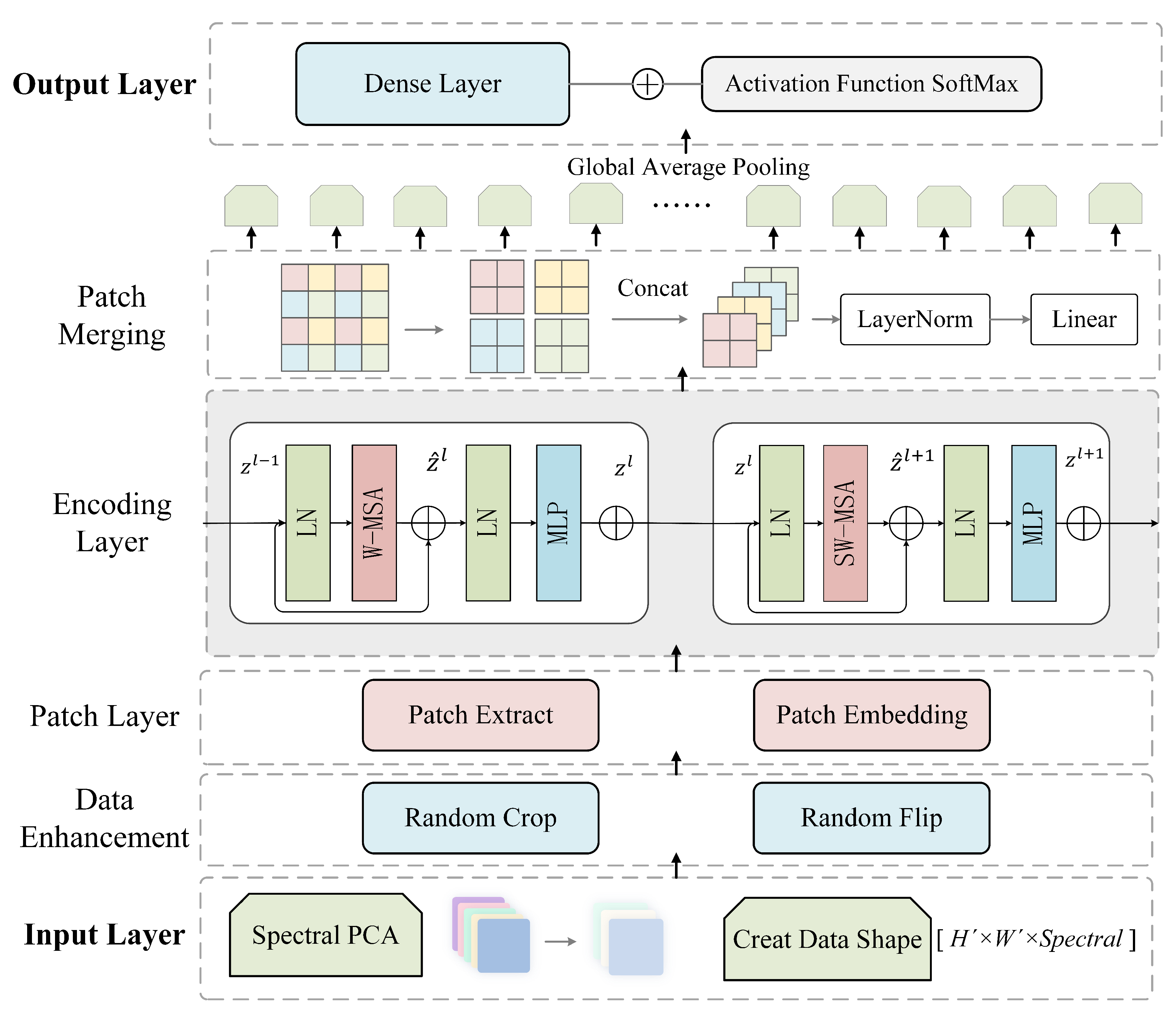
2.1. Spectral Swin Transformer Network for HSI Classification

Figure 1 shows the structural diagram of the model proposed in this paper. Firstly, we used PCA to reduce the spectral dimensions of the hyperspectral data at the input layer of the model. The spectra of hyperspectral images are typically high-dimensional and redundant. The PCA can project the spectral dimensions onto a new low-dimensional space, thereby removing redundant information and extracting the most important features, making the data more easily processed and classified. This is why PCA plays an important role in hyperspectral image classification; it is an effective feature extraction and data compression method.

Then, a data cube was created with three dimensions: width, height, and the simplified spectral dimension. The function “Create Image Cubes” extracts image patches of a specified size from an input image and creates corresponding labels. It pads the image with zeros, iterates over each pixel, and stores the surrounding image patches in an array. If desired, it can remove patches with zero labels and adjust the labels accordingly. The function’s main purpose is to facilitate the extraction of image patches and their associated labels for further analysis or processing. The data features are enhanced, and the cube is divided into patches at the patch layer. The input shape of a model is positively correlated with its computational complexity. A smaller input shape allows for higher-resolution hyperspectral images to be processed by the model, but may result in reduced classification accuracy. In the context of scientific research, it is important to consider the trade-off between the input shape and classification accuracy when working with hyperspectral images.

The Swin Transformer is a computer vision algorithm based on ViT [21]. It introduces an innovative sliding window mechanism that limits the attention mechanism to a fixed window size, allowing the model to learn features that span the window. The hierarchical design of the subsampling layer enables the model’s self-attentive mechanism, taking into account both local and global features of the data. The performance of the Swin Transformer tends to vary greatly with different types of datasets. Transformers often achieve good training results on large datasets but are less effective when dealing with a limited number of training samples. Therefore, the Swin Transformer designs schemes with different window sizes for different dataset types and sizes. We refer to the Swin Transformer’s tiny universal backbone network in the official Microsoft example (accessed on 30 April 2023. https://github.com/microsoft/Swin-Transformer). To improve computing efficiency, simplify the structure, and adapt to HSI classification, we reduce redundant linear embedding and patch-merging modules, compared to the normal Swin Transformer structure. We cut it down from four stages to one.

Random crop is the most commonly used data augmentation method in deep learning, which can enhance the model’s accuracy and stability. Random flip is a data augmentation method that randomly flips the matrix during training. Patch extraction is the process of further extracting the enhanced features of the data. The patch-embedding module crops the feature data with patch sizes (the initial setting is 2) to the window size settings and embeds them in each patch.

The function of the patch-merging module is to subsample before the beginning of each stage, narrow the resolution, adjust the number of channels and, thus, form a hierarchical design. Finally, the global average pooling layer will obtain the output features with the softmax activation function corresponding to different classes. Global average pooling outputs 1D data, which replaces the full connection layer in the popular CNN model and avoids model overfitting.

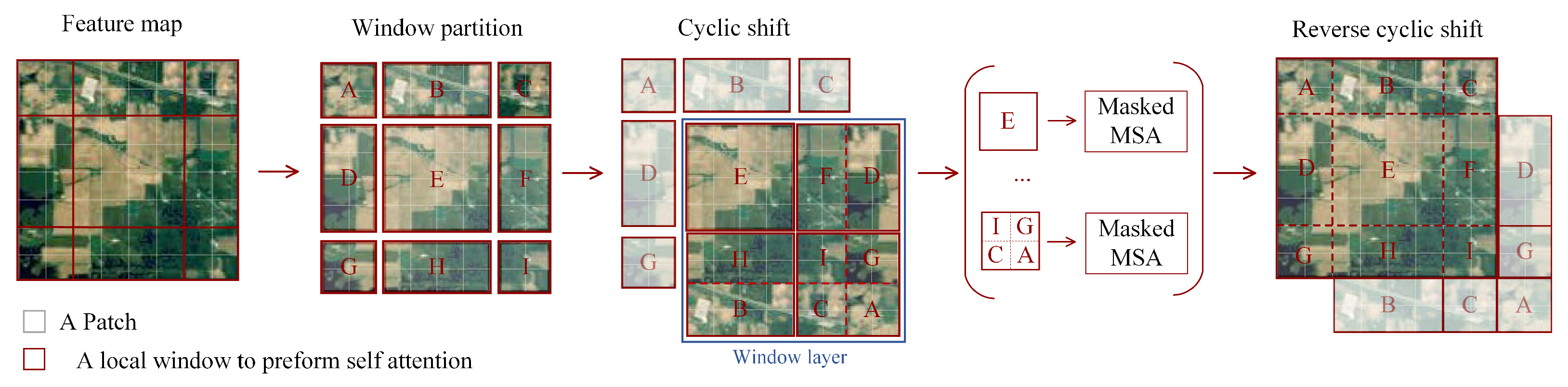
2.2. Swin Transformer Encoder and SW-MSA

Two successive Swin Transformer blocks are the core of the Swin Transformer, which introduces shifted window operations that interact with other windows. The computations of two successive Swin Transformer blocks can be expressed as in Equation (1). The features that are input in this stage, $z^{l-1}$, go through layer normalization (LN), window multi-head self-attention (W-MSA), and the residual layer, to obtain ${\widehat{z}}^l$. After going through LN and multilayer perceptron (MLP) again, it enters the second block that has shifted window multi-head self-attention (SW-MSA).

$$\begin{array}{c}\hfill {\widehat{z}}^l=W-MSA\left(LN\left(z^{l-1}\right)\right)+MSA\left(LN\left(Z^{l-1}\right)\right)+z^{l-1}\\ \hfill z^{l+1}=MLP\left(LN\left({\widehat{z}}^{l+1}\right)\right)+{\widehat{z}}^{l+1}{z}^l=MLP\left(LN\left({\widehat{z}}^l\right)\right)+{\widehat{z}}^l\\ \hfill {\widehat{z}}^{l+1}=SW-MSA\left(LN\left(z^l\right)\right)+MSA\left(LN\left(Z^l\right)\right)+Z^l\end{array}$$

(1)

The attention weight calculation for each partitioned window is defined by Formula (2). V is the relative position encoding of Q, K. The dot products of Q and K represent their similarity, but the similarity is not normalized. Therefore, a softmax function is applied to normalize the dot products of Q and K. The resulting softmax output is a mask matrix with all values ranging from 0 to 1. V represents the linearly transformed features of the input. Multiplying the mask matrix with V results in a filtered V feature.

$$Attention(Q,K,V)=Softmax\left(\frac{Q{K}^T}{\sqrt{d}}\right)V$$

(2)

Shifted window multi-head self-attention (SW-MSA) can send self-attention calculations across the four windows in the window layer. A schematic diagram of the shifted window offset process can be seen in Figure 2. For each patch in the feature map, it is necessary to calculate all the patches in the self-attention calculation process. Shifted W-MSA modules first divided the feature map into multiple windows based on the $M\times M$ size, cyclic-shift offset windows, and self-attention for each internal window. By setting reasonable masks, we reduce the computation amount in each window (Figure 2 shows that there are four windows inside the window layer).

2.3. Parametric Analysis

To verify the effectiveness of the proposed model in HSI classification, several important parameters were selected, and the method of controlling variables was used to examine the impact on the final test accuracy. The Swin Transformer architecture is based on ViT, so module parameters that are not present in ViT were selected to demonstrate the effectiveness of the Swin Transformer in the field of HSI classification. The window size and shift stride are particularly important parameters. The attention head numbers are also important parameters that affect the computational complexity of the model.

In the early feature-processing stage of the proposed model, the patch size and spectral dimensions were experimentally determined. The larger the selected values, the higher the real-time computational load of the model, while smaller values require longer computation times. Additionally, different HSI datasets require different patch-input sizes, with the optimal range being between 5 and 25. The reduced spectral dimension ranges from 10 to 30.

We use the Indian pine HSI dataset as an example. In

Table 1. Analysis of the effect of the setting of the number of parameters on the final accuracy of the proposed model. (Indian Pine dataset).

Numbers	Attention Heads	Attention Window	Shifting Window	S-T Block
0				88.61%
1	97.13%	98.21%	97.46%	96.19%
2	97.48%	97.46%	97.37%	97.46%
4	97.63%	98.46%	97.54%
8	97.46%

, it can be observed that the model’s accuracy decreases when the number of Swin Transformer modules is reduced or when the Swin Transformer (S-T) block is not used. Changing the number of attention heads in the model has minimal impact on the accuracy, with the default parameter being 8. The default parameter for the size of the attention window is 2, and the default parameter for the size of the shifting window is 1. Larger window sizes and window shift strides may cause the model to overlook some local features, ultimately affecting the classification accuracy.

3. Experimental Results

3.1. Dataset Description

The Indian Pine dataset and the Salinas University dataset, which are publicly available on the Internet, were used as part of the dataset for this experiment. To demonstrate the generalization ability of our model, we also utilized other publicly available hyperspectral datasets from various regions in China. These datasets include three hyperspectral datasets from different areas in Wuhan City, Hubei Province (Honghu, Hanchuan, and Longkou) [24,25,26,27]. Additionally, we utilized the MaTiWan Village hyperspectral dataset [28] from XiongAn(XA) New Area, Hebei Province. The majority of these datasets contain various types of crops as the main objects of study. Information on how to obtain the data will be provided in the data availability statement.

The Indian Pine (IP) dataset was collected by the AVIRIS sensor at a site in northwest Indiana. It has an image size of $145\times 145$ pixels and a spatial resolution of 0.2 m. After removing 20 absorbing water bands, the number of bands is 200. Sixteen feature classes are labeled in the available ground truth.

The Salinas (SA) dataset was collected by AVIRIS in 1998 at Salinas Valley, California, USA. After removing 20 bands with a low signal-to-noise ratio (SNR), 204 bands were used for the experiment. The HSI includes $512\times 217$ pixels with a spatial resolution of 3.7 m. Sixteen common categories are labeled in the ground truth.

The University of Pavia (PU) dataset is a part of the hyperspectral data images created in 2003 in Pavia, Italy. This dataset has 103 hyperspectral images after band denoising. There were 42,776 pixels containing ground truth and nine categories.

The WHU-Hi dataset comprises three separate unmanned aerial vehicle (UAV)-based hyperspectral datasets: WHU-Hi-Longkou (LK), WHU-Hi-HanChuan (HC), and WHU-Hi-HongHu (HU). Compared to satellite and airborne hyperspectral platforms, UAV-based hyperspectral systems can acquire high-spatial-resolution hyperspectral images.

The first dataset, WHU-Hi-HongHu, was collected in Honghu City on 20 November 2017, using a Headwall Nano-Hyperspec imaging sensor mounted on a DJI Matrice 600 Pro UAV platform. The experimental area is a complex agricultural scene with many crop types, including Chinese cabbage, cabbage, Brassica chinensis, and small Brassica chinensis. The dataset contains 270 bands ranging from 400 to 1000 nm, with a spatial resolution of 0.043 m.

The second dataset, WHU-Hi-HanChuan, was collected in Hanchuan on 17 June 2016, using a similar imaging sensor mounted on a Leica Aibot X6 UAV V1 platform. The study area was a rural–urban fringe zone with buildings, water, and cultivated land, and contains seven crop species: strawberry, cowpea, soybean, sorghum, water spinach, watermelon, and greens. The dataset contains 274 bands ranging from 400 to 1000 nm, with a spatial resolution of 0.109 m. Notably, due to the low solar elevation angle during data collection, there are many shadow-covered areas in the image.

The third dataset, WHU-Hi-LongKou, was collected in Longkou Town on 17 July 2018, using a Headwall Nano-Hyperspec imaging sensor mounted on a DJI Matrice 600 Pro UAV platform. The study area is a simple agricultural scene with six crop species: corn, cotton, sesame, broadleaf soybean, narrow-leaf soybean, and rice. The dataset contains 270 bands ranging from 400 to 1000 nm, with a spatial resolution of 0.463 m.

The aerial hyperspectral remote sensing image from the XA New Area of Matihewan Village has a spectral range of 400–1000 nm, with 250 bands, an image size of 3750 × 1580 pixels, and a spatial resolution of 0.5 m. Through the field investigation of ground object categories, a total of 19 annotated ground object categories were identified in this image, primarily consisting of economic crops.

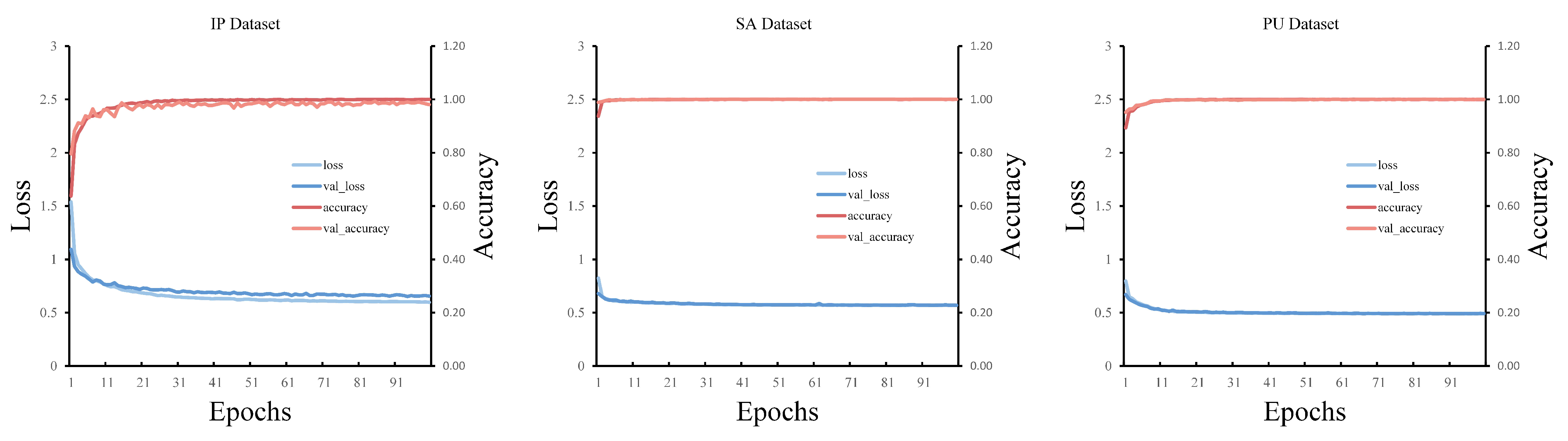
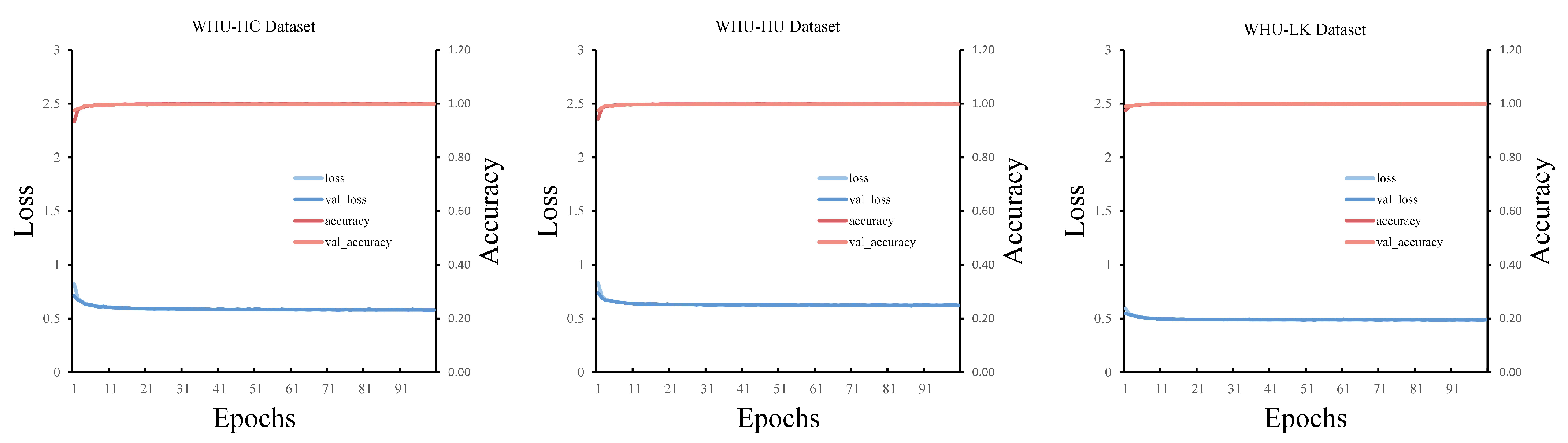
3.2. Training Details and Evaluation Indicators

This paper utilized a laptop computer equipped with an NVIDIA GeForce GTX1060 graphics card(Model: Y7000, Lenovo China) and a cloud server with an NVIDIA GTX3090 graphics card(Provider: AutoDL, China. Accessed on 30 April 2023 https://www.autodl.com/home), which were responsible for processing small-scale and high-resolution datasets, respectively. The datasets were divided into a training set, comprising 30% of the data and a testing set comprising 70% of the data. The learning rate was set to 0.001.

The initial patch size for feature extraction was set to 25, which is a crucial parameter that affects the computational time and performance of the CPU and GPU. A larger value requires a higher performance from the computer, while a smaller value results in a longer computation time. Therefore, it is essential to strike a balance between the initial patch size and the training performance. A patch size of 25 was found to perform well on most datasets, but it was not suitable for the high-resolution XA dataset, which required a smaller patch size to allow for the computation on our cloud server.

In the Swin Transformer model, we used initial parameters with a patch size of 2 × 2, a dropout rate of 0.03, 8 attention heads, an embedding dimension of 64, 256 multilayer perceptrons, a window size of 2, and a shift window step of 1. The model uses TensorFlow 2.9 and Python 3.8. In this study, the AdamW optimizer and stochastic gradient descent (SGD) optimizer trained our proposed Swin Transformer model. Categorical cross-entropy was chosen as the loss function. In the experiment, we found that different optimizers would affect the final accuracy of the model, so we prepared a comparison of the results of different optimizers.

This experiment used three prevalence evaluation metrics: average accuracy (AA), overall accuracy (OA), and kappa coefficient. Average accuracy represents the average of the classification accuracy of each class and is calculated in Equations (3) and (4).

$$Recall=\frac{Truepositive}{(Truepositive+Falsenegative)}$$

(3)

$$AA=\frac{{\sum }_{i=1}^{n}Recal{l}_i}{n}\times 100$$

(4)

$$OA=\frac{(Truepositive+TrueNegative)}{Totalnumberofpixels}\times 100$$

(5)

$$Kappa=\frac{p_0-p_e}{1-p_e},p_0=\frac{\sum x_{ii}}{N},p_e=\frac{\sum x_i+x_i+\cdots }{N^2}$$

(6)

Overall accuracy was calculated in Equation (5). Kappa (6) is a statistical measure that provides consistent mutual information between the tip of the ground truth map and the classification map. $P_o$ is the observed agreement, which refers to the classification consistency among evaluators and classifiers. $P_e$ is the expected chance agreement, which is the expected level of agreement by chance based on the predicted distribution of the classifier, where $X_i+$ is the marginal total number of observations in row I, the total number of observations is N, and $X_{ii}$ is the number of observations in row I, column I.

3.3. Classification Results of Public Hyperspectral Image Datasets

The classification results of the Indian Pine (IP) hyperspectral dataset, the Pavia University (PU) hyperspectral dataset, and the Salinas (SA) hyperspectral dataset in our model are shown in Figure 3. In the figure, it can be observed that our proposed model achieved relatively high test accuracies on all three datasets. Additionally, the loss convergence was faster on the SA and PU datasets. This corresponds to the results of the parameter analysis discussed in Section 2. This is because the spectral dimension of the IP dataset was set to 30, while the spectral dimension of the SA and PU datasets was set to 15. The spectral dimension of the WHU-HI dataset was also set to 15, which resulted in good performance, as seen in Figure 4. The XA dataset has a higher resolution, and when creating its input data cube shape, smaller data had to be used. However, even with this consideration, the classification performance did not improve significantly, with an average test accuracy of only about 48% in Figure 5.

3.4. Classification Results for Each Object Class in All HSI Datasets

Table 2. IP dataset classification results, including class, precision, recall, and F1 score.

	Precision	Recall	F1 Score	Support
Alfalfa	0.79	0.97	0.87	32
Corn—no-till	0.97	0.95	0.96	1000
Corn—min-till	0.97	0.98	0.98	581
Corn	0.96	0.98	0.97	166
Grass–pasture	0.95	0.96	0.95	338
Grass–trees	0.96	0.98	0.97	511
Grass—pasture-mowed	0.75	0.45	0.56	20
Hay—windrowed	1.00	1.00	1.00	335
Oats	1.00	0.29	0.44	14
Soybean—no-till	0.96	0.95	0.96	680
Soybean—min-till	0.98	0.99	0.99	1719
Soybean—clean	0.94	0.96	0.95	415
Wheat	0.97	0.99	0.98	143
Woods	1.00	1.00	1.00	886
Buildings–Grass–Trees–Drives	1.00	1.00	1.00	270
Stone–Steel–Towers	0.87	0.63	0.73	65

,

Table 3. SA dataset classification results, including class, precision, recall, and F1 score.

	Precision	Recall	F1 Score	Support
Broccoli_green_weeds_1	1.00	1.00	1.00	1406
Broccoli_green_weeds_2	1.00	1.00	1.00	2608
Fallow	1.00	1.00	1.00	1383
Fallow_rough_plow	1.00	1.00	1.00	976
Fallow_smooth	1.00	1.00	1.00	1875
Stubble	1.00	1.00	1.00	2771
Celery	1.00	1.00	1.00	2505
Grapes_untrained	1.00	1.00	1.00	7890
Soil_vineyard_develop	1.00	1.00	1.00	4342
Corn_senesced_green_weeds	1.00	1.00	1.00	2295
Lettuce_romaine_4wk	1.00	1.00	1.00	748
Lettuce_romaine_5wk	1.00	1.00	1.00	1349
Lettuce_romaine_6wk	1.00	1.00	1.00	641
Lettuce_romaine_7wk	1.00	1.00	1.00	749
Vineyard_untrained	1.00	1.00	1.00	5088
Vineyard_vertical_trellis	1.00	1.00	1.00	1265

,

Table 4. PU dataset classification results, including class, precision, recall, and F1 score.

	Precision	Recall	F1 Score	Support
Asphalt	1.00	1.00	1.00	4642
Meadows	1.00	1.00	1.00	13,055
Gravel	1.00	1.00	1.00	1469
Trees	1.00	1.00	1.00	2145
Painted metal sheets	1.00	1.00	1.00	942
Bare Soil	1.00	1.00	1.00	3520
Bitumen	1.00	1.00	1.00	931
Self-Blocking Bricks	1.00	1.00	1.00	2577
Shadows	1.00	1.00	1.00	663

,

Table 5. HC dataset classification results, including class, precision, recall, and F1 score.

	Precision	Recall	F1 Score	Support
Strawberry	1.00	1.00	1.00	31,315
Cowpea	1.00	1.00	1.00	15,927
Soybean	1.00	1.00	1.00	7201
Sorghum	1.00	1.00	1.00	3747
Water spinach	1.00	1.00	1.00	840
Watermelon	1.00	0.97	0.98	3173
Greens	1.00	1.00	1.00	4132
Trees	1.00	1.00	1.00	12,585
Grass	1.00	1.00	1.00	6628
Red roof	1.00	1.00	1.00	7361
Gray roof	1.00	1.00	1.00	11,838
Plastic	1.00	1.00	1.00	2575
Bare soil	0.99	0.99	0.99	6381
Road	1.00	1.00	1.00	12,992
Bright object	1.00	1.00	1.00	795
Water	1.00	1.00	1.00	52,781

,

Table 6. HU dataset classification results, including class, precision, recall, and F1 score.

	Precision	Recall	F1 Score	Support
Red roof	1.00	1.00	1.00	9829
Road	1.00	0.98	0.99	2458
Bare soil	1.00	1.00	1.00	15,275
Cotton	1.00	1.00	1.00	114,300
Cotton firewood	1.00	1.00	1.00	4353
Rape	1.00	1.00	1.00	31,190
Chinese cabbage	1.00	1.00	1.00	16,872
Pak choi	1.00	1.00	1.00	2838
Cabbage	1.00	1.00	1.00	7573
Tuber mustard	1.00	1.00	1.00	8676
Brassica parachinensis	1.00	1.00	1.00	7711
Brassica chinensis	1.00	1.00	1.00	6268
Small Brassica chinensis	1.00	1.00	1.00	15,755
Lactuca sativa	0.99	1.00	1.00	5149
Celtuce	1.00	0.99	0.99	701
Film covered lettuce	1.00	1.00	1.00	5083
Romaine lettuce	1.00	1.00	1.00	2107
Carrot	0.99	1.00	0.99	2252
White radish	1.00	1.00	1.00	6098
Garlic sprouts	1.00	1.00	1.00	2440
Broad bean	1.00	0.99	1.00	930
Tree	1.00	1.00	1.00	2828

,

Table 7. LK dataset classification results, including class, precision, recall, and F1 score.

	Precision	Recall	F1 Score	Support
Corn	1.00	1.00	1.00	24,158
Cotton	1.00	1.00	1.00	5862
Sesame	1.00	1.00	1.00	2122
Broadleaf soybean	1.00	1.00	1.00	44,248
Narrow-leaf soybean	1.00	1.00	1.00	2906
Rice	1.00	1.00	1.00	8298
Water	1.00	1.00	1.00	46,939
Roads and houses	0.99	0.99	0.99	4987
Mixed weed	1.00	0.98	0.99	3660

and

Table 8. XA dataset classification results, including class, precision, recall, and F1 score.

	Precision	Recall	F1 Score	Support
Acer negundo Linn	0.34	0.10	0.15	157,953
Willow	0.34	0.41	0.37	126,536
Elm	0.00	0.00	0.00	10,747
Paddy	0.47	0.52	0.49	316,501
Chinese Pagoda Tree	0.39	0.47	0.43	332,914
Fraxinus chinensis	0.37	0.45	0.40	118,539
Koelreuteria paniculata	0.00	0.00	0.00	16,313
Water	0.33	0.00	0.00	115,953
Bare land	0.00	0.00	0.00	26,886
Paddy stubble	0.35	0.15	0.21	135,681
Robinia pseudoacacia	0.00	0.00	0.00	3928
Corn	0.67	0.00	0.00	41,416
Pear	0.62	0.93	0.74	718,559
Soya	0.00	0.00	0.00	5006
Alamo	0.39	0.05	0.10	63,750
Vegetable field	0.00	0.00	0.00	20,404
Sparsewood	0.00	0.00	0.00	1047
Meadow	0.47	0.54	0.50	295,253
Peach	0.00	0.00	0.00	45,860
Building	0.15	0.00	0.00	20,731

show the classification results with AdamW for each class, including precision, recall, and F1 score. Accuracy is a metric that evaluates the proportion of correctly classified samples among all predicted samples. The F1 score is a statistical measure that assesses the accuracy of a binary classification model, taking into account both its precision and recall. The F1 score can be viewed as a weighted average of the model’s precision and recall, with a range of values between 0 and 1.

3.5. Classification Maps and Comparisons

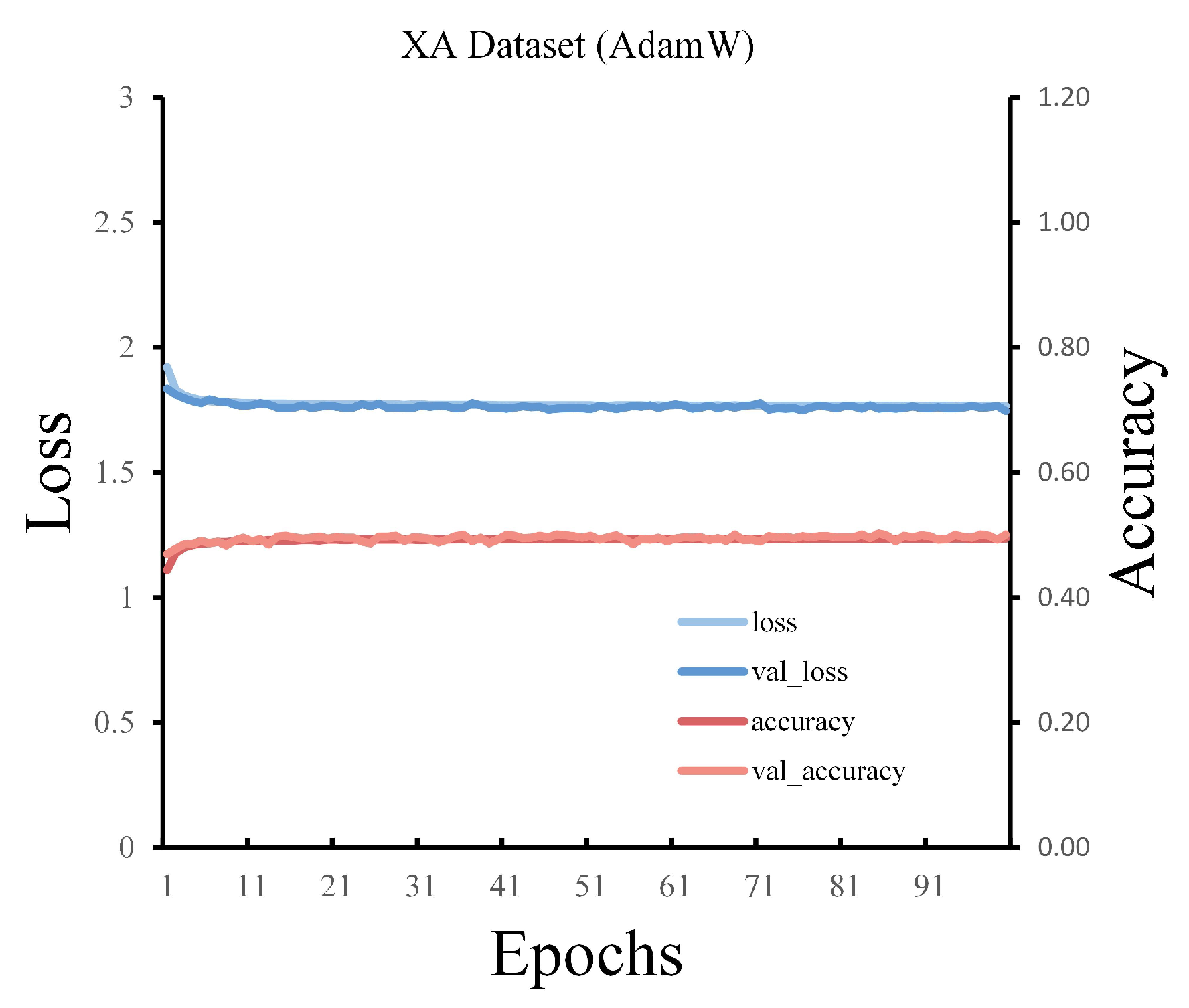
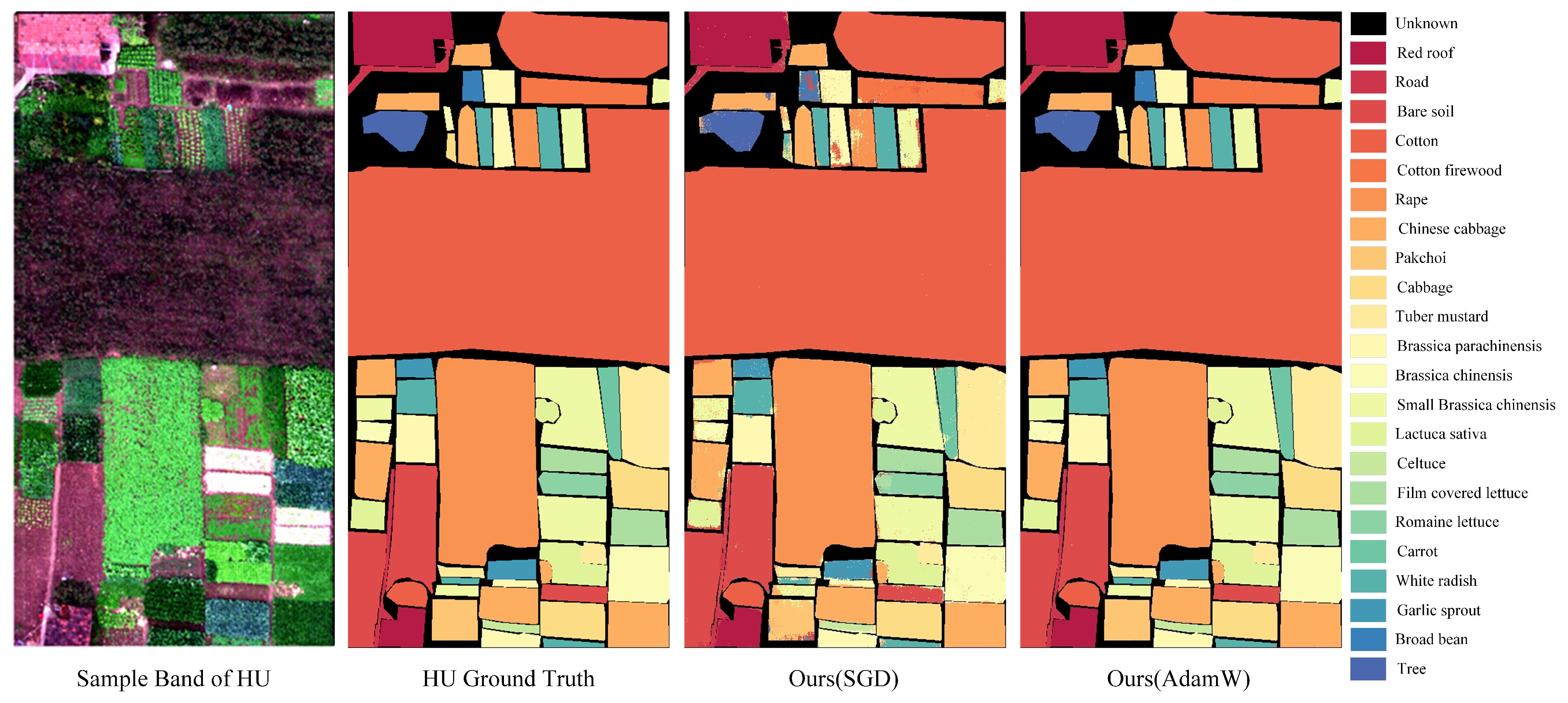
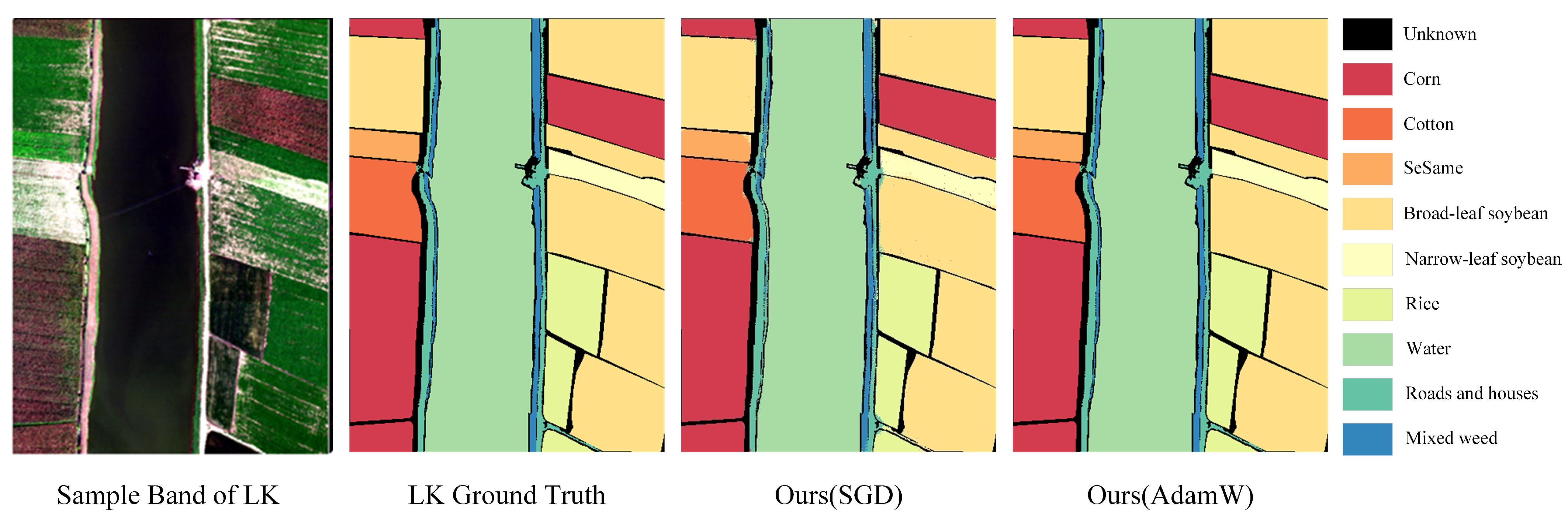
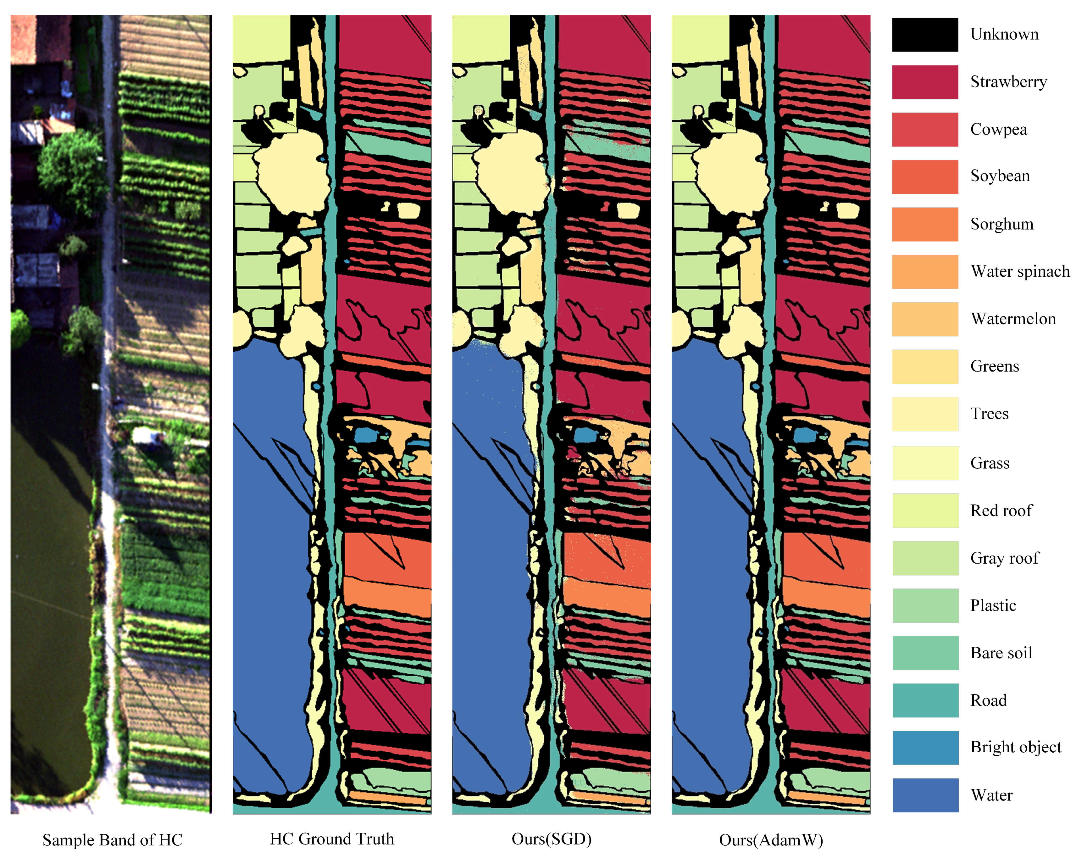
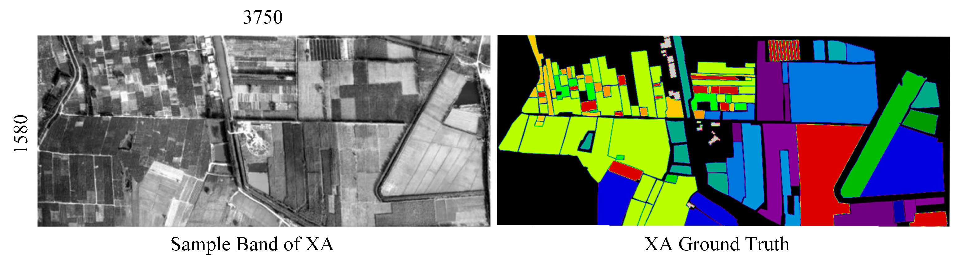
3.5.1. Classification Maps of Chinese Dataset: (WHU-HI and XA Datasets)

To demonstrate the generalization ability of our model, we also tested it on other uncommon hyperspectral datasets, including three datasets from Wuhan and the XA dataset. For the Honghu dataset in Wuhan, which has a relatively high resolution, we reduced the patch size from 25 to 17 and set the spectral dimension to 15. For the XA dataset, which has the highest resolution, both the patch size and spectral dimension were reduced to 5 and 10, respectively.

As shown in Figure 6, Figure 7 and Figure 8, to highlight the differences in classification performance, we added the results of different optimizers on the WHU-HI dataset to demonstrate the variation in classification. It can be observed from the figure that the AdamW optimizer performs significantly better in the classification map compared to the SGD optimizer. Therefore, the choice of optimizer is crucial in deep learning models and has a significant impact on the final results. Due to the limited availability of hyperspectral datasets in China, there is relatively little research on classification models for these datasets. Therefore, there is no comparison of the classification performances of these datasets in different models. Since the XA dataset is too large to yield classification maps in our proposed model, Figure 9 only shows the original and correctly categorized maps of the XA dataset. In this paper, we only discuss the results obtained by training our model on these hyperspectral datasets. These datasets will be submitted together with the data availability statement.

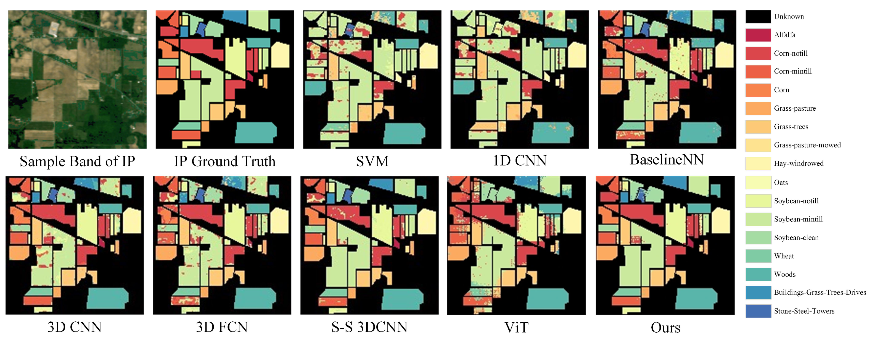
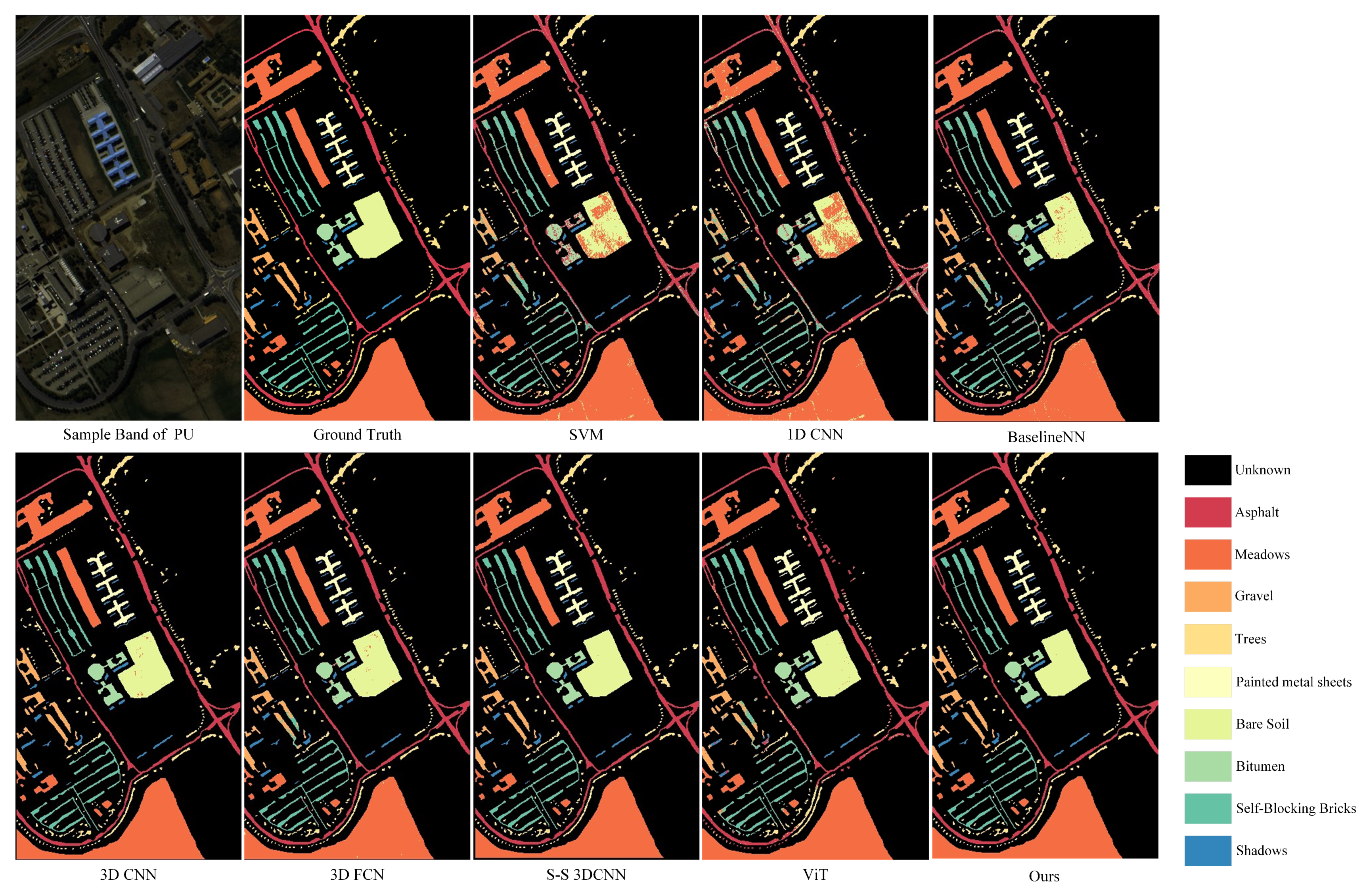
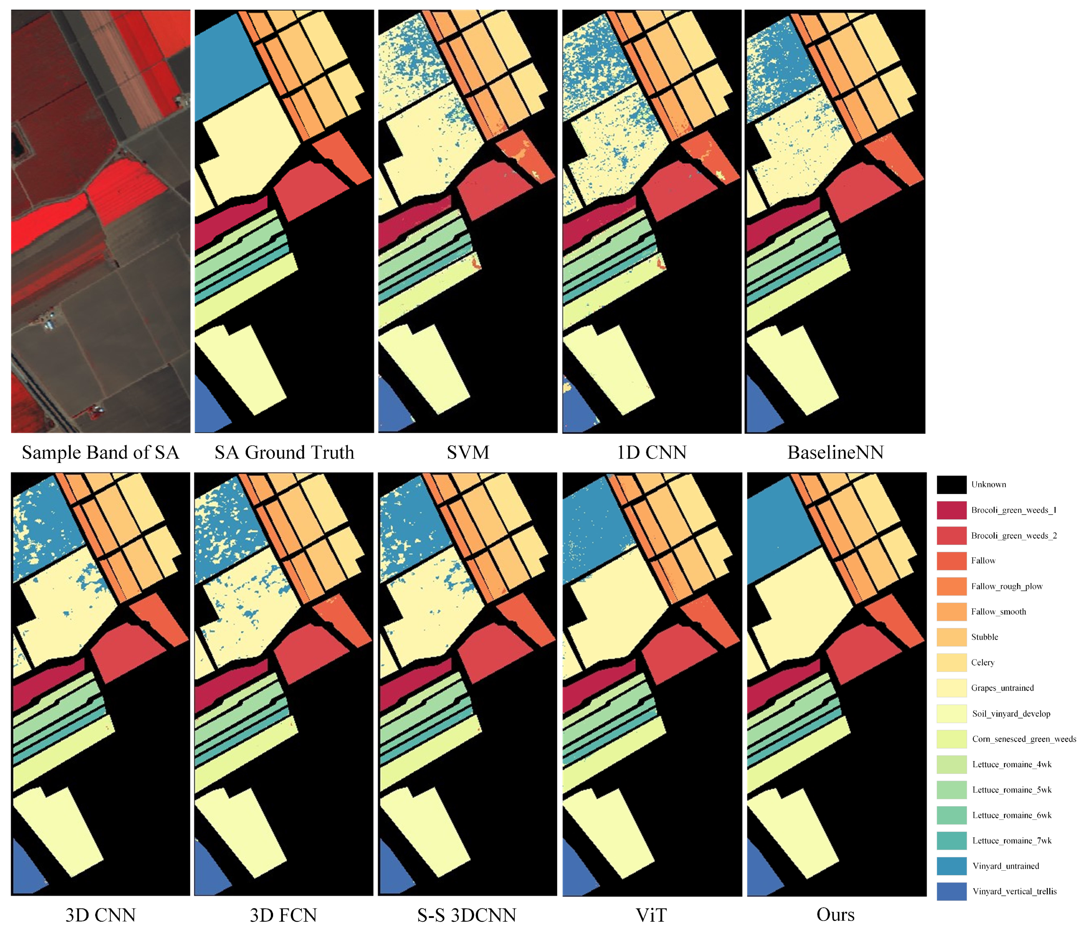
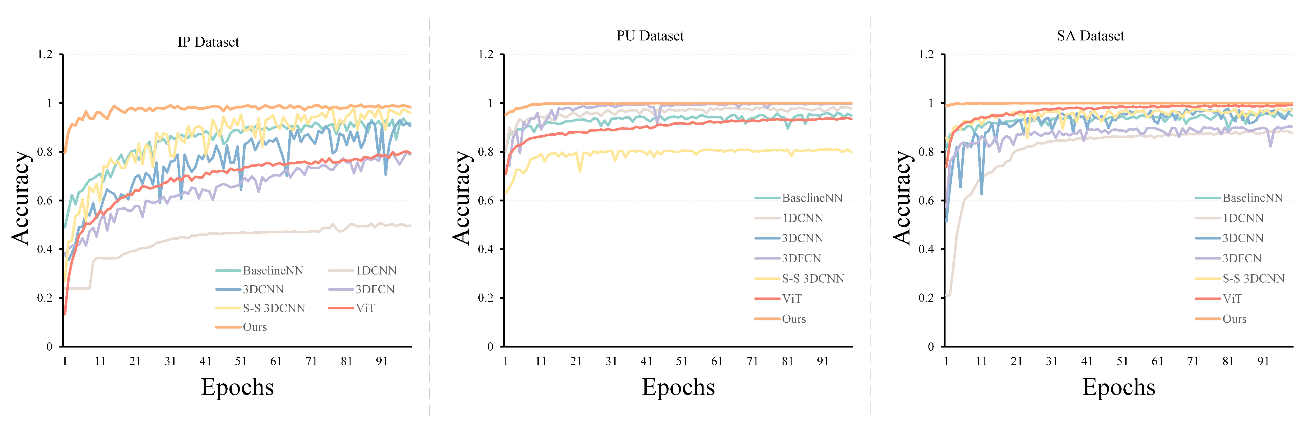
3.5.2. Comparison of Our Proposed Model with Other Models on IP, SA, and PU Hyperspectral Datasets

Different from the current mainstream CNN architecture, this study uses an advanced Swin Transformer to propose a novel HSI classification model. To verify the effectiveness of the proposed method, we compare the classification results with the HSI classification classical models SVM [29], Baseline NN [29], 1DCNN [30], 2DCNN [31], 3DCNN [32], and the mainstream models 3DFCN [33], spatial–spectral 3DCNN(S-S 3DCNN) [34], ViT [21,35], and spatial–spectral ViT (SST) [22]. The code for comparative experiments was obtained from an open-source code collection on GitHub [29] (accessed on 30 April 2023 https://github.com/nshaud/DeepHyperX). The comparative experiment was conducted with a learning rate of 0.001 and a training set size of 30%, while the test set size was 70%, which is the same as in our model. All other parameters were set to their default values, as specified in the comparative code. The comparative results presented below are based on 100 training iterations and include the results obtained using the AdamW optimizer in our model.

Figure 10, Figure 11 and Figure 12 show the classification prediction maps of the ground truth samples for the IP, PU, and SA hyperspectral datasets, respectively, using various models. The maps include the real ground sample images and the correct classification answers. By comparison, we found that the 3D neural network-based model achieved good results because it can perform feature convolution in three dimensions simultaneously. However, in our model, we achieved similarly excellent results even without using three-dimensional convolution. The ground sample details in the classification results of SA and PU were well-classified and superior to those of the classical machine learning methods. However, in the case of the IP dataset, our model did not achieve the expected results, which we attribute to the input shape of the model.

Figure 13 presents a comparison of the classification results of various algorithms for the IP, PU, and SA datasets, using models referenced in the experimental setup section, with all parameters except for the learning rate set to their default values. Our model was configured with a patch size of 25 and spectral dimensions of 30 and 15, with the latter used for datasets with higher resolution (>500). The results show that our model achieved classification accuracy comparable to other state-of-the-art models in the PU and SA datasets when using the AdamW optimizer.

Table 9. Classification accuracy comparison between the proposed model and other models on the IP dataset with 30% training data. (×100%).

	Methods	Average Accuracy	Overall Accuracy	Kappa
ML Models	SVM	0.317	0.528	0.427
	Baseline NN	0.654	0.753	0.713
DL Models	1D CNN	0.203	0.449	0.324
	3D CNN	0.663	0.775	0.737
	3D FCN	0.545	0.702	0.658
	S-S 3D CNN	0.744	0.779	0.749
ViT Models	ViT	0.789	0.718	0.680
	S-S ViT	0.667	0.887	0.864
	Ours	0.880	0.972	0.969

,

Table 10. Comparison of the classification accuracy between the proposed model and other models on the SA dataset with 30% training data. (×100%).

	Methods	Average Accuracy	Overall Accuracy	Kappa
ML Models	SVM	0.317	0.528	0.427
	Baseline NN	0.908	0.917	0.908
DL Models	1D CNN	0.809	0.832	0.812
	3D CNN	0.879	0.911	0.901
	3D FCN	0.904	0.939	0.932
	S-S 3D CNN	0.908	0.947	0.941
ViT Models	ViT	0.753	0.781	0.709
	S-S ViT	0.931	0.942	0.937
	Ours	0.999	0.999	0.999

and

Table 11. Comparison of the classification accuracy between the proposed model and other models on the PU dataset with 30% training data. (×100%).

	Methods	Average Accuracy	Overall Accuracy	Kappa
ML Models	SVM	0.635	0.834	0.771
	Baseline NN	0.852	0.961	0.948
DL Models	1D CNN	0.585	0.781	0.696
	3D CNN	0.857	0.954	0.939
	3D FCN	0.867	0.976	0.968
	S-S 3D CNN	0.876	0.969	0.959
ViT Models	ViT	0.769	0.802	0.701
	S-S ViT	0.836	0.927	0.908
	Ours	0.999	0.999	0.999

provide a comparison of the OA, AA, and kappa results for each algorithm, revealing that our model achieved good classification accuracy and competitive performance. Our model achieved significant advantages in the SA and PU datasets. It outperforms traditional machine learning (ML) methods and is also highly competitive in deep learning (DL) methods and Vision Transformers. Almost all models perform better in the SA and PU datasets compared to the IP dataset.

4. Conclusions

This paper mainly introduces a Swin Transformer network for processing three-dimensional HSI data. By reducing the spectral dimensionality through PCA in the preliminary stage and combining spectral information to create a three-dimensional data cube, it mitigates the high-dimensionality and complexity of high-spectral-resolution data. Finally, the unique shift window and global self-attention computation in the Swin Transformer are combined for high-spectral-resolution image classification. Experimental results demonstrate competitive performance on most small-scale HSI datasets.

In the experiments, it is observed that a less complex network structure is sufficient for handling small-scale HSI datasets. Many studies focus on adding more modules to tackle different complex problems. In HSI classification tasks, if the early-stage feature processing is conducted properly, even a simple structure can yield good results, as demonstrated by the HybridSN [36] architecture. However, such a structure has a limitation in handling ultra-high-resolution HSI datasets, performing poorly when faced with high-spectral-resolution datasets exceeding 1000 pixels. How to handle large-scale HSI datasets is a question that we will need to research in the future. The proposed model also provides a good approach for HSI classification models based on Vision Transformer.

References

1. Teke, M.; Deveci, H.S.; Haliloğlu, O.; Gürbüz, S.Z.; Sakarya, U. A short survey of hyperspectral remote sensing applications in agriculture. In Proceedings of the 2013 6th International Conference on Recent Advances in Space Technologies (RAST), Istanbul, Turkey, 12–14 June 2013; pp. 171–176. [Google Scholar]
2. Shafri, H.Z.; Taherzadeh, E.; Mansor, S.; Ashurov, R. Hyperspectral remote sensing of urban areas: An overview of techniques and applications. Res. J. Appl. Sci. Eng. Technol. 2012, 4, 1557–1565. [Google Scholar]
3. Bedini, E. The use of hyperspectral remote sensing for mineral exploration: A review. J. Hyperspectral Remote Sens. 2017, 7, 189–211. [Google Scholar] [CrossRef]
4. Lu, G.; Fei, B. Medical hyperspectral imaging: A review. J. Biomed. Opt. 2014, 19, 010901. [Google Scholar] [CrossRef] [PubMed]
5. Hughes, G. On the mean accuracy of statistical pattern recognizers. IEEE Trans. Inf. Theory 1968, 14, 55–63. [Google Scholar] [CrossRef] [Green Version]
6. Rodarmel, C.; Shan, J. Principal component analysis for hyperspectral image classification. Surv. Land Inf. Sci. 2002, 62, 115–122. [Google Scholar]
7. Du, H.; Qi, H.; Wang, X.; Ramanath, R.; Snyder, W.E. Band selection using independent component analysis for hyperspectral image processing. In Proceedings of the 32nd Applied Imagery Pattern Recognition Workshop, Washington, DC, USA, 15–17 October 2003; pp. 93–98. [Google Scholar]
8. Gogineni, R.; Chaturvedi, A. Hyperspectral image classification. Process. Anal. Hyperspectral Data 2019. [Google Scholar] [CrossRef] [Green Version]
9. Kuo, B.C.; Yang, J.M.; Sheu, T.W.; Yang, S.W. Kernel-based KNN and Gaussian classifiers for hyperspectral image classification. In Proceedings of the IGARSS 2008—2008 IEEE International Geoscience and Remote Sensing Symposium, Boston, MA, USA, 7–11 July 2008; pp. II-1006–II-1008. [Google Scholar] [CrossRef]
10. Mercier, G.; Lennon, M. Support vector machines for hyperspectral image classification with spectral-based kernels. In Proceedings of the IGARSS 2003. 2003 IEEE International Geoscience and Remote Sensing Symposium. Proceedings (IEEE Cat. No. 03CH37477), Toulouse, France, 21–25 July 2003; Volume 1, pp. 288–290. [Google Scholar]
11. Kuo, B.C.; Ho, H.H.; Li, C.H.; Hung, C.C.; Taur, J.S. A kernel-based feature selection method for SVM with RBF kernel for hyperspectral image classification. IEEE J. Sel. Top. Appl. Earth Obs. Remote Sens. 2013, 7, 317–326. [Google Scholar] [CrossRef]
12. Tarabalka, Y.; Fauvel, M.; Chanussot, J.; Benediktsson, J.A. SVM-and MRF-based method for accurate classification of hyperspectral images. IEEE Geosci. Remote Sens. Lett. 2010, 7, 736–740. [Google Scholar] [CrossRef] [Green Version]
13. Li, S.; Song, W.; Fang, L.; Chen, Y.; Ghamisi, P.; Benediktsson, J.A. Deep learning for hyperspectral image classification: An overview. IEEE Trans. Geosci. Remote Sens. 2019, 57, 6690–6709. [Google Scholar] [CrossRef] [Green Version]
14. Lee, H.; Kwon, H. Going deeper with contextual CNN for hyperspectral image classification. IEEE Trans. Image Process. 2017, 26, 4843–4855. [Google Scholar] [CrossRef] [Green Version]
15. Yu, S.; Jia, S.; Xu, C. Convolutional neural networks for hyperspectral image classification. Neurocomputing 2016, 219, 88–98. [Google Scholar] [CrossRef]
16. Mei, X.; Pan, E.; Ma, Y.; Dai, X.; Huang, J.; Fan, F.; Du, Q.; Zheng, H.; Ma, J. Spectral-Spatial Attention Networks for Hyperspectral Image Classification. Remote Sens. 2019, 11, 963. [Google Scholar] [CrossRef] [Green Version]
17. Mengmeng, Z.; Wei, L.; Qian, D. Diverse region-based CNN for hyperspectral image classification. IEEE Trans. Image Process. 2018, 27, 2623–2634. [Google Scholar]
18. Wan, S.; Gong, C.; Zhong, P.; Du, B.; Zhang, L.; Yang, J. Multiscale dynamic graph convolutional network for hyperspectral image classification. IEEE Trans. Geosci. Remote Sens. 2019, 58, 3162–3177. [Google Scholar] [CrossRef] [Green Version]
19. Jiao, L.; Liang, M.; Chen, H.; Yang, S.; Liu, H.; Cao, X. Deep fully convolutional network-based spatial distribution prediction for hyperspectral image classification. IEEE Trans. Geosci. Remote Sens. 2017, 55, 5585–5599. [Google Scholar] [CrossRef]
20. Gong, Z.; Zhong, P.; Yu, Y.; Hu, W.; Li, S. A CNN with multiscale convolution and diversified metric for hyperspectral image classification. IEEE Trans. Geosci. Remote Sens. 2019, 57, 3599–3618. [Google Scholar] [CrossRef]
21. Dosovitskiy, A.; Beyer, L.; Kolesnikov, A.; Weissenborn, D.; Zhai, X.; Unterthiner, T.; Dehghani, M.; Minderer, M.; Heigold, G.; Gelly, S.; et al. An image is worth 16x16 words: Transformers for image recognition at scale. arXiv 2020, arXiv:2010.11929. [Google Scholar]
22. He, X.; Chen, Y.; Lin, Z. Spatial-Spectral Transformer for Hyperspectral Image Classification. Remote Sens. 2021, 13, 498. [Google Scholar] [CrossRef]
23. Liu, Z.; Lin, Y.; Cao, Y.; Hu, H.; Wei, Y.; Zhang, Z.; Lin, S.; Guo, B. Swin Transformer: Hierarchical Vision Transformer using shifted windows. In Proceedings of the IEEE/CVF International Conference on Computer Vision, Online, 11–17 October 2021; pp. 10012–10022. [Google Scholar]
24. Bei, Z.; Yanfei, Z.; Liangpei, Z.; Bo, H. The Fisher Kernel Coding Framework for High Spatial Resolution Scene Classification. Remote Sens. 2016, 8, 157. [Google Scholar]
25. Zhao, B.; Zhong, Y.; Xia, G.S.; Zhang, L. Dirichlet-derived multiple topic scene classification model for high spatial resolution remote sensing imagery. IEEE Trans. Geosci. Remote Sens. 2015, 54, 2108–2123. [Google Scholar] [CrossRef]
26. Zhu, Q.; Zhong, Y.; Zhao, B.; Xia, G.S.; Zhang, L. Bag-of-visual-words scene classifier with local and global features for high spatial resolution remote sensing imagery. IEEE Geosci. Remote Sens. Lett. 2016, 13, 747–751. [Google Scholar] [CrossRef]
27. Zhong, Y.; Hu, X.; Luo, C.; Wang, X.; Zhao, J.; Zhang, L. WHU-Hi: UAV-borne hyperspectral with high spatial resolution (H2) benchmark datasets and classifier for precise crop identification based on deep convolutional neural network with CRF. Remote Sens. Environ. 2020, 250, 112012. [Google Scholar] [CrossRef]
28. Cen, Y.; Zhang, L.; Zhang, X.; Wang, Y.; Qi, W.; Tang, S.; Zhang, P. Aerial hyperspectral remote sensing classification dataset of Xiongan New Area (Matiwan Village). J. Remote. Sens. 2020, 24, 1299–1306. Available online: https://www.ygxb.ac.cn/en/article/doi/10.11834/jrs.20209065/ (accessed on 1 May 2023).
29. Audebert, N.; Le Saux, B.; Lefèvre, S. Deep learning for classification of hyperspectral data: A comparative review. IEEE Geosci. Remote Sens. Mag. 2019, 7, 159–173. [Google Scholar] [CrossRef] [Green Version]
30. Hu, W.; Huang, Y.; Wei, L.; Zhang, F.; Li, H. Deep convolutional neural networks for hyperspectral image classification. J. Sens. 2015, 2015, 258619. [Google Scholar] [CrossRef] [Green Version]
31. Liu, B.; Yu, X.; Zhang, P.; Tan, X.; Yu, A.; Xue, Z. A semi-supervised convolutional neural network for hyperspectral image classification. Remote Sens. Lett. 2017, 8, 839–848. [Google Scholar] [CrossRef]
32. Hamida, A.B.; Benoit, A.; Lambert, P.; Amar, C.B. 3-D deep learning approach for remote sensing image classification. IEEE Trans. Geosci. Remote Sens. 2018, 56, 4420–4434. [Google Scholar] [CrossRef] [Green Version]
33. Lee, H.; Kwon, H. Contextual deep CNN based hyperspectral classification. In Proceedings of the 2016 IEEE International Geoscience and Remote Sensing Symposium (IGARSS), Beijing, China, 10–15 July 2016; pp. 3322–3325. [Google Scholar]
34. Li, Y.; Zhang, H.; Shen, Q. Spectral–spatial classification of hyperspectral imagery with 3D convolutional neural network. Remote Sens. 2017, 9, 67. [Google Scholar] [CrossRef] [Green Version]
35. Ayas, S.; Tunc-Gormus, E. SpectralSWIN: A spectral-Swin Transformer network for hyperspectral image classification. Int. J. Remote Sens. 2022, 43, 4025–4044. [Google Scholar] [CrossRef]
36. Roy, S.K.; Krishna, G.; Dubey, S.R.; Chaudhuri, B.B. HybridSN: Exploring 3-D–2-D CNN feature hierarchy for hyperspectral image classification. IEEE Geosci. Remote Sens. Lett. 2019, 17, 277–281. [Google Scholar] [CrossRef] [Green Version]
Figure 1. The proposed model’s Swin Transformer structure.
Remotesensing 15 03721 g001
Figure 2. Self-attention computation in shifted window partitioning.
Remotesensing 15 03721 g002
Figure 3. The accuracy and loss of the IP, SA, and PU datasets in our model were trained for 100 epochs.
Remotesensing 15 03721 g003
Figure 4. The accuracy and loss of the WHU-HI datasets in our model were trained for 100 epochs.
Remotesensing 15 03721 g004
Figure 5. The accuracy and loss of the XA dataset in our model were trained for 100 epochs.
Remotesensing 15 03721 g005
Figure 6. Classification maps of the HU hyperspectral dataset.
Remotesensing 15 03721 g006
Figure 7. Classification maps of the LK hyperspectral dataset.
Remotesensing 15 03721 g007
Figure 8. Classification maps of the HC hyperspectral dataset.
Remotesensing 15 03721 g008
Figure 9. XA dataset ground sample and truth information.
Remotesensing 15 03721 g009
Figure 10. Comparison of classification maps between various algorithms and the proposed algorithm in the IP hyperspectral dataset.
Remotesensing 15 03721 g010
Figure 11. Comparison of classification maps between various algorithms and the proposed algorithm in the PU hyperspectral dataset.
Remotesensing 15 03721 g011
Figure 12. Comparison of classification maps between various algorithms and the proposed algorithm in the SA hyperspectral dataset.
Remotesensing 15 03721 g012
Figure 13. Comparison of model validation accuracy in the IP, PU, and SA datasets.
Remotesensing 15 03721 g013