Article

Improving the Spatial Prediction of Sand Content in Forest Soils Using a Multivariate Geostatistical Analysis of LiDAR and Hyperspectral Data

by
Annamaria Castrignanò
1,
Gabriele Buttafuoco
2,*,
Massimo Conforti
3,
Mauro Maesano
4,
Federico Valerio Moresi
4 and
Giuseppe Scarascia Mugnozza
4
1
Department of Engineering and Geology (InGeo), Gabriele D’Annunzio University of Chieti-Pescara, 66100 Chieti, Italy
2
National Research Council of Italy, Institute for Agriculture and Forestry Systems in the Mediterranean (CNR-ISAFOM), Via Cavour 4/6, 87036 Rende, Italy
3
National Research Council of Italy, Research Institute for Geo-Hydrological Protection (CNR-IRPI), Via Cavour 4/6, 87036 Rende, Italy
4
Department of Innovation in Biology, Agri-Food and Forest Systems (DIBAF), University of Tuscia, Via San Camillo de Lellis SNC, 01100 Viterbo, Italy
*
Author to whom correspondence should be addressed.
Remote Sens. 2023, 15(18), 4416; https://doi.org/10.3390/rs15184416
Submission received: 22 August 2023 / Revised: 4 September 2023 / Accepted: 5 September 2023 / Published: 7 September 2023
(This article belongs to the Special Issue Remote Sensing in Geomatics)

Abstract

:
Soil sand particles play a crucial role in soil erosion because they are more susceptible to being detached and transported by erosive forces than silt and clay particles. Therefore, in soil erosion assessment and mitigation, it is crucial to model and predict soil sand particles at unsampled locations using appropriate methods. The study was aimed to evaluate the ability of a multivariate approach based on non-stationary geostatistics to merge LiDAR and visible-near infrared (Vis-NIR) diffuse reflectance data with laboratory analyses to produce high-resolution maps of soil sand content. Remotely sensed, high-resolution LiDAR-derived topographic attributes can be used as auxiliary variables to estimate soil textural particle-size fractions. The proposed approach was compared with the commonly used univariate approach of ordinary kriging to evaluate the contribution of auxiliary variables. Soil samples (0–0.20 m depth) were collected at 135 locations within a 139 ha forest catchment with granitic parent material and subordinately alluvial deposits, where soils classified as Typic Xerumbrepts and Ultic Haploxeralf crop out. A number of linear trend models coupled with different auxiliary variables were compared. The best model for predicting sand content was the one with elevation derived from LIDAR data as the only auxiliary variable. Although the improvement in estimation over the univariate model was rather marginal, the proposed approach proved very flexible and scalable to include any type of auxiliary variable. The application of LiDAR data is expected to expand as it allows the high-resolution prediction of soil properties, generally insufficiently sampled, at different spatial scales.

Graphical Abstract

1. Introduction

Many functions are carried out by soil, ensuring a fundamental contribution to human life and well-being; however, to understand the potential of soil in providing functions, it is necessary to characterize the variability of soil properties in space and time [1]. Soil texture is one of the most important properties that influence many soil functions, such as water cycling, and processes, such as soil erosion or aggregation, through both the absolute values of its properties and their spatial variability [2]. Generally, soils with high sand contents also have low organic carbon contents [3], and sand particles are more susceptible than finer ones (silt and clay) to being detached and transported by erosive forces [4]. In sandy soils within mountainous and forested areas with varying morphology, modeling and predicting sand content at unsampled locations is, therefore, crucial to assess soil erosion and design measures for its mitigation.
Since direct laboratory measurements are generally expensive and time-consuming, different types of soil sensing technologies, from diffuse reflectance spectroscopy to proximal and remote sensing, although indirect measures, can provide rapid and reliable information on soil property variability at different spatial and temporal scales [5,6,7]. However, data measured in laboratories and/or with different soil sensing methods require their fusion and integration [8,9,10]. A proper integrated use or synthesis (fusion) of different spatial data results in a more informative result than the one coming from individual sources and provides new knowledge, understanding, and explanations of the processes [11,12,13].
When modeling and mapping topsoil, there has always been a compromise between the need to produce models of high spatial resolution but limited extent (at the local scale) and the need to produce models of coarse spatial resolution but wide extent (as at the regional or country scale) [14]. Large-scale spatial soil models at high resolution could fill the gap of knowledge and reduce the uncertainty in soil modeling, as well as allow the inclusion and understanding of all necessary physical and biological processes that take place on the Earth’s surface [15]. Morphometric attributes such as elevation, slope gradient, aspect, local relief, and slope curvature have been commonly used to estimate the surface lithology and model the spatial variability of soils [16,17]. Actually, topography, together with climate and land cover, is one of the main factors that influence soil properties and determine its heterogeneity at many scales [18].
However, most of these studies used digital elevation models with a spatial resolution greater than 10 m. Although such a scale may be suitable for some environmental studies, it may be unsuitable for accurately describing the spatial variability of highly changing landscapes [19], such as the characteristic landscapes of the forested mountains of some Calabrian areas in southern Italy [20].
One of the most important recent developments in remote sensing for lithological mapping of the soil surface is the increasing availability of high-resolution digital elevation models (DEMs) derived from LiDAR (Light Detection and Ranging) elevation data. The high density of measurement points obtained from a LiDAR sensor allows for precision mapping of land surface features and also makes it possible to clearly distinguish soil from vegetation [14]. LiDAR data are widely used to study landscape and topography [21], tree attributes [20], phenotyping, and biomass [20], but they can also be used to assess soil properties [22].
It is widely recognized that there are various advantages, including economic ones, that would result from the use of LiDAR data in predicting soil lithology [14]. The use of LiDAR data makes it possible to cover vast areas that are morphologically impervious and even difficult to access and to construct DEMs with high spatial resolution [23]. Recently, the DEM resolution derived by LiDAR data has increased, reaching even 0.5 m with the use of airplanes [24] up to very accurate resolutions (~0.03 m) using the drone [25]. Airborne laser scanning (ALS) is the most highly accurate and efficient method to acquire 3D data from large areas and to generate DEMs, such as the Digital Terrain Model (DTM) and the Digital Surface Model (DSM). Moreover, using geographic information systems (GIS) algorithms, these new high-resolution elevation data can be used to provide several primary and secondary topographic attributes.
It is widely accepted that a larger number of soil samples can more accurately describe and model spatial heterogeneity. To overcome the generally limited resources of the budget for soil measurements, soil spectroscopy techniques, such as visible-near-infrared spectroscopy (Vis-NIR, 350–2500 nm), can be used to estimate soil properties such as the different particle sizes (clay, silt, and sand), organic and inorganic carbon concentrations, and iron concentrations quickly, accurately, and relatively inexpensively [26,27,28]. This allows the use of soil data from hyperspectral spectroscopic measurements appropriately reduced in dimensions as an additional source of information supplementing direct laboratory soil measurements in order to improve the prediction of the variable of interest [29].
To produce soil maps associated with some measure of prediction uncertainty by efficiently combining heterogeneous data, several techniques spanning from traditional spatial statistics and geostatistics to machine learning have been used in recent decades [30,31,32]. Actually, the different computing technologies lead to a single formulation, which makes it possible to model the spatial variability of any soil property on different spatial scales, separating the deterministic component (trend at the long scale) from the stochastic one (at the short or local scale) [33]. Geostatistics describes the spatial patterns and provides estimates of attributes at unsampled locations [34]. Its most common linear interpolator under stationary (i.e., no trend) conditions is ordinary kriging, which uses only the variable of interest [35]. Non-geostatistical techniques (multi-linear regression or machine learning) have generally been used to describe the trend, while geostatistical techniques quantify the stochastic component of variability [36]. These two types of approaches can be kept separate or combined in hybrid techniques (non-stationary geostatistics) [37]. An efficient hybrid technique is kriging with external drift [35,38], in which the trend is externally modeled by auxiliary variables and the trend and residuals are simultaneously estimated in a single system with a jointly calculated covariance function. However, the trend of the target variable or some of its transformation functions must be expressed by linear models. It therefore follows from the above that the joint analysis of a variety of spatially correlated data of different types requires a proper method of data processing.
The objectives of the study were (1) to define a multivariate approach based on non-stationary geostatistics to merge remotely sensed high-resolution LiDAR-derived topographic attributes with Vis-NIR diffuse reflectance spectroscopy and laboratory data to produce high-resolution maps of soil sand content and its estimation uncertainty, and (2) to evaluate the advantage of using LiDAR data over employing the univariate model of ordinary kriging to estimate the soil sand content.

2. Materials and Methods

2.1. Study Area

The study area is the Bonis catchment, situated in the upland landscape of the Sila Massif (Figure 1), Calabria Region (southern Italy), which is an important site for investigating the effect of forest management on its hydrologic behavior. Due to its location, the installed instrumentation, and its forest cover, the Bonis catchment has been studied intensively for many years [20,39,40,41]. The catchment has an area of 140 hectares, and its altitude varies from 1019 to 1341 m a.s.l., with a mean value of 1130 m a.s.l. (Figure 1). The forest cover is mainly characterized by Pinus nigra ssp. laricio (Poir.) Maire (about 95 hectares), whereas the remaining 45 hectares are formations of Castanea sativa Mill, riparian vegetation, and a small portion of bare soil.
In the catchment, Palaeozoic granitoid rocks crop out, which are deeply fractured and weathered and often covered with thick layers of saprolite and/or colluvial deposits [41]. The landscape is predominantly characterized by rugged morphology with steep slopes, often cut by deep incisions [41]. The slope gradient varies from 0° to 50°, with a mean value of 21°. According to the Calabria Soil Map [42], the soils of the study area can be classified as Typic Xerumbrepts and Ultic Haploxeralf [43]. The dominant soil textural classes are sandy loam and sandy clay loam. The upper A-horizon often shows a very dark brown color due to the accumulation of organic matter (umbric epipedon). Regarding the pedo-climate features, the study area is characterized by a mesic soil temperature regime and an udic soil moisture regime [42].
The climate of the study area is typical of Calabrian mountainous areas, with a long-term average precipitation of about 1080 mm and an average temperature of about 0.1 °C in the coldest month and 18.3 °C in the warmest month. The climate data were provided by the Multi-Risk Functional Centre of the Regional Agency for Environment Protection of the Calabria Region and recorded at the Cecita station (UTM zone 33N; easting = 633,373 m; northing = 4,360,500 m), located a few km from the study area.

2.2. Remote Sensing (LiDAR) Data Acquisition and Processing

At the study site, the light detection and ranging (LiDAR) scanning system was used by airborne laser scanning (ALS) to provide a high-quality point cloud and density.
The measurement was made with a Riegl LMS-Q560 laser scanner with a frequency of 400,000 Hz, a FOV of 60°, and an inclination of 20° mounted on a helicopter operating at approximately 700 m above ground level. The LiDAR sensor has been set up to obtain the resulting point cloud at about 20 points per square meter to attain the accuracy of producing DEM layers with 1 m resolution. The World Geodetic System 1984 (WGS 84) and Universal Transversal Mercator (UTM) projection (zone 33N) coordinate systems were assigned to the cloud points. The LiDAR data used in this research were acquired in 2017 as part of a national project [20].
To derive the DEM accurately, the raw point cloud acquired by the sensor must be processed to remove unwanted points from laser range scans and obtain the cleaned point cloud. The LiDAR data were processed using the commercial software LiDAR360 version 6.0 (Green Valley International Inc., Berkeley, CA, USA), and the data have been archived in the LAS (LASer) format.
The workflow to generate the terrain models involves several steps. The first one is to check the data quality and remove isolated points and noise through denoising. The Remove Outliers tool in LiDAR360 was used to remove the noise and improve the quality of the data. The tool analyzes the average distance to all neighboring points and determines the average and standard deviation for each point to identify outliers and remove them from the data. Once outliers have been removed from the point cloud, the next step is to classify ground points through the Classify Ground Points tool in LiDAR360 and set up the value 2 for the ground points, as defined by the American Society for Photogrammetry and Remote Sensing (ASPRS) for Standard LiDAR Point Classes. After this, the DEM tool was used to create the raster of the DTM with 1-m resolution using the Inverse Distance Weighting (IDW) interpolation method.

2.3. Topographic Attributes

Elevation, slope, aspect, curvature, length-slope (LS) factor, stream power index (SPI), and topographic wetness index (TWI) were the topographic attributes used as auxiliary variables in the geostatistics analysis to produce high-resolution maps of soil sand content distribution. These topographic attributes were derived by the LiDAR–DTM, using the SAGA-GIS software version 8.2.1 [44]. Details on the calculation of the topographic attributes can be found in Wilson and Gallant [45] or Florinsky [46]. The distribution of soil properties can be influenced by elevation because it affects the local microclimate by changing the patterns of temperature, precipitation, and soil moisture [47]. The slope gradient is a morphometric attribute of primary importance in the processes governing both pedogenesis and soil erosion/deposition; in fact, it influences surface runoff, soil infiltration, and the intensity of erosion processes [45,48,49]. The aspect plays a fundamental role in controlling soil moisture along the slopes through solar radiation and rainfall as well as in influencing many factors regulating soil formation processes and soil productivity [45,47]. Slope curvature provides information on slope shape; it is important for soil mapping because it influences local superficial water flow in terms of convergence or divergence and acceleration or deceleration of the flow across the surface. The LS factor is a variable used in the RUSLE equation to consider the effect of topography on soil erosion [50]. It depends on slope steepness factor (S) and slope length (L); it influences surface runoff intensity and is considered a sediment transport capacity index. The SPI attribute is a measure of the erosive power of overland flow based on the assumption that discharge is proportional to the specific catchment area [51]. Generally, the higher the value of SPI, the higher the likelihood of water soil erosion. The TWI attribute indicates the effects of local topography on hydrological processes [45]. It is an index of the likelihood of a cell collecting water and is considered a predictor of soil saturation. It exerts a great influence on hillslope processes such as soil and water redistribution and vertical infiltration. Finally, TRI is a morphometric indicator that describes whether the topography of an area is flat or undulated and represents the spatial variability of a landscape. It may be used to measure the variation in elevation between neighboring spatial pixels of a DEM [45].

2.4. Field Soil Sampling and Laboratory Analysis

A field survey was conducted to collect 135 topsoil (0–0.20 m depth) samples within the Bonis catchment (Figure 1), with a density of almost one sample per hectare. At each sampling location, surface litter was removed, and soil was sampled using a metallic core cylinder having a diameter of 0.075 m and a height of 0.20 m. The position of the soil sampling sites was acquired using a hand-held GNSS device with a precision of about 1 m.
The soil samples were transferred to the laboratory in polyethylene bags, dried at 40 °C in a ventilated oven, homogenized, and then sieved using a 2-mm mesh stainless steel sieve. Successively, the sieved samples were used for soil particle size measurement with the hydrometer method after a pre-treatment with sodium hexametaphosphate as a dispersing agent [52]. According to the USDA [53] classification for soil texture, sand, silt, and clay particle sizes were categorized as follows: 0.05–2.0 mm for sand, 0.002–0.05 mm for silt, and 0.002 mm for clay. In addition, the soil samples were finely sieved through a 0.25 mm mesh sieve, and SOC concentration was determined by dry combustion using a Shimadzu TOC-L analyzer with an SSM-5000A solid sample module (Shimadzu Corporation, Kyoto, Japan). Each measurement was made in triplicate, and the soil sample was re-measured if the standard deviation of the three replicates exceeded 2.5%.

2.5. Hyperspectral Spectroscopy Measurements

The visible near-infrared (Vis-NIR) reflectance spectroscopy analysis was performed in a laboratory using an ASD FieldSpec IV spectroradiometer (Analytical Spectral Devices Inc., Boulder, CO, USA) with a spectral range of 350–2500 nm. The spectral measurements were performed in a dark room to reduce the effect of external light, with the spectroradiometer held in the nadir position at a distance of 0.10 m from the soil sample. A 50 W halogen lamp with a zenith angle of 30° at a distance of 0.25 m from the sample was used [26]. Each soil sample was placed in a Petri dish (0.09 m in diameter and 0.01 m deep), and the surface of the soil was leveled with a spatula [41]. Before starting the soil sample measurements, dark current was removed, and the spectroradiometer was calibrated with a white panel of known reflectance (Spectral on Diffuse Reflectance Panel). Generally, the calibration was repeated once every 20 min.
For each soil sample, 50 scans were acquired, which were then averaged to obtain the soil spectrum. To reduce the noise level and external interference, the diffuse reflectance spectra were pre-processed by means of a nine-point smoothing function [54], using the ViewSpecpro software version 3.2 (Malvern Panalytical Ltd., Malvern, UK). Finally, each soil spectrum was resampled every 10 nm wavelength to reduce the total number of raw reflectance bands and avoid overfitting [55].

2.6. Preliminary Statistical Data Analysis and Non-Stationary Geostatistical Approach

An exploratory data analysis was carried out for all study variables before applying the geostatistical approach. The main basic statistics were calculated (minima, medians, means, maxima, standard deviations, and skewness and kurtosis coefficients), and those variables with a significant deviation from the Gaussian distribution (probably due to large outliers) were transformed to the standardized normal distribution. To do that, a set of Hermite polynomials truncated to the first 100 terms was used to estimate the Gaussian anamorphosis function of transformation [35]. At the end, the Gaussian estimates were back-transformed to the raw values by using the above Gaussian anamorphosis function [56].

2.6.1. Principal Component Analysis

Principal component analysis (PCA) [57] is a method of analysis for multivariate data that is widely used because of the simplicity of its algebra and straightforward interpretation [37]. Moreover, it is frequently applied in remote sensing to reduce the dimensionality of radiometric variables recorded by multi- or hyperspectral radiometers. The principal components (PCs) are calculated as the eigenvectors of the correlation matrix [58] and are not then directly observable variables, for which they require to be interpreted from a scientific-rational perspective. Mathematically, they are expressed as a linear combination of the observed variables and are of the same number. Actually, only a part of them is necessary, and namely, those with eigenvalues greater than 1 determine the number of retained PCs (Kaiser’s criterion) [59]. The results can be subjected to rotation by a variety of methods to improve the interpretation of PCs. Those employing orthogonal rotations are preferred as they preserve the statistical independence of the PCs. In this study, the VARIMAX procedure was used, and the values of the loading coefficients were multiplied by 100 and rounded to the nearest integer, and those with absolute values greater than 68.73 (the root mean square of all the values multiplied by 100 in the matrix of PC loadings) were plotted in a graph.
PCA was performed on the pretreated reflectance spectroscopy data with the SAS/FACTOR procedure of the statistical software package SAS/STAT version 9.2 [60] in order to reduce the number of variables (250 raw diffuse reflectance bands).

2.6.2. Fusion of Heterogeneous Spatial Data

Two data sets were required to apply the non-stationary geostatistical technique known as kriging with external drift (KED) [45,48] to estimate the soil sand content at the nodes of the interpolation grid (mesh = 1 m). The latter was based on the digital elevation model (DEM) obtained from the LiDAR data.
The first of these is the co-regionalization data set (vector file of points), including the sand content (target variable) data and all the auxiliary variables (external variables for KED) measured/calculated at the 135 soil sampling locations and used to calculate the trend.
The second one is the interpolation data set (raster file) based on a 1-m mesh DEM at whose nodes all the auxiliary variables have been calculated or estimated.
Preliminarily to the realization of the two aforementioned data sets, it was necessary to apply fusion techniques since the data to be processed were of different types and not in the same spatial location (not collocated): (1) scattered sample data (at 135 locations): clay and soil organic carbon (SOC); (2) sample data at the same 135 locations but consisting of diffuse reflectance spectra discretized into 216 wavelength intervals and to which principal component analysis (PCA) was applied in order to reduce their size to a few principal components (PCs); and (3) raster data at the 1-m DEM nodes (elevation and all derived topographic attributes).
For the realization of the collocated point data set, a migration of the raster data from the pixel to the nearest sample location was therefore necessary. Differently for the raster data set, the point data were required to be interpolated at the grid nodes, using ordinary kriging for clay content and SOC data and ordinary cokriging [35] for the principal components (PCs) of spectroscopy data.
For an in-depth description of the basic geostatistical techniques, such as the Linear Model of Coregionalization (LMC), kriging, and cokriging. Interested readers are referred to the numerous manuals on the subject [35,37,61]. Following, there is a brief description of the main statistical and geostatistical procedures used in this work.

2.6.3. Kriging with External Drift

Non-stationary geostatistics is applied in cases where the target variable exhibits systematic variations (trend or drift), so that estimation of the variogram model may be problematic or, in some cases, impossible. The variogram is a mathematical model that describes the spatial continuity of the attributes of interest and measures the average dissimilarity between observations depending on separation distance and direction [61]. Its main features are summarized by two parameters: sill and range. Generally, after an initial increase, the variogram will reach a maximum (sill variance) at a finite lag distance (range), which is the distance over which pairs of values are spatially correlated [61]. Moreover, the variogram can show a discontinuity at its origin, called the nugget effect, which characterizes the very short-scale variability within the shortest sampling interval and the error variance [61]. In the non-stationary case, the sill is increasing without any finite distance within the study area. Non-stationary geostatistical techniques (universal kriging, UK, and kriging with external drift, KED) [35] are based on the assumption that a generic random variable is constituted by a deterministic component plus a random component. Universal kriging represents the trend as a linear combination of generally polynomial functions of the coordinates, while KED is a linear combination of independent external variables. However, combinations of the two trend types are also possible.
To treat non-stationary cases, Matheron [62] introduced the kriging of intrinsic random functions of order k (IRF-k), which essentially consists of two steps: (1) trend identification, and (2) determination of the spatial structure of residuals through the definition of generalized spatial covariance models using higher order increments compared with the linear increments of ordinary kriging. In this way, the trend can be completely filtered out, and thus stationarity is again achieved [35]. Reference is made to the text cited before [62] and to other publications on the subject [40] for a complete description of the theory. Only the main operational steps for producing the spatial maps of the estimated variable of interest and estimation uncertainty will be outlined below.
Unlike universal kriging, in IRF-k theory it is not necessary to know the coefficients of the trend but only its order, which is generally assumed to be less than or equal to 2.
Structural analysis, according to this theory, consists of two steps:
(1)
Determination of the order k of the trend;
(2)
Calculation of the generalized covariance function K(h) of the module of the distance vector (h) and fitting of an authorized parametric model to it.
The order of the trend (k) corresponds to the degree of the polynomial used to describe the large-scale variation (i.e., at a scale longer than the size of the study area). For determining the degree of trend, the least-squares errors corresponding to the various polynomials of degrees 0, 1, and 2 are calculated for each sampling point. The degree corresponding to the minimum error is assigned rank 1, and that with the maximum error is assigned rank 3. The ranks for each degree are finally averaged over all sample points, and the degree corresponding to the smallest average rank is assumed to be the optimal degree for the trend.
In this procedure, the neighborhood is split into two rings: the closest samples to the target sample belong to ring number 1, and the other samples belong to ring number 2. Fitting is based on a cross-validation procedure. All the data from ring 1 are used to fit the functions corresponding to the different trend hypotheses. Each datum of ring 2 is used to evaluate the quality of the fit. Then the roles of both rings are inverted. The best fit corresponds to the minimal average variance of the cross-validation errors.
A convenient model for generalized covariance functions is the polynomial model given by the linear combination of a given set of generic basic structures. All possible combinations can be reduced in practice to a combination of four basic models with terms arranged according to increasing regularity [35]:
K ( h ) = C 0   δ ( h ) b 0 h + b S h 2 log h + b 1 h 3
where δ(h) = 0 for h = 0, otherwise δ(h) = 1. The coefficients C0, b0, bs, and b1 in a two-dimensional space R2, must satisfy the following set of inequalities for K(h) to be a valid generalized covariance of IRF-k (authorized model):
C 0 0 , b 0 0 , b 1 0 , b S 3 2   b 0 b 1
Unlike the variogram, the generalized covariance function cannot be estimated directly, but depends on knowing the order of the trend in the IRF-k theory.
The procedure for selecting the generalized covariance function is based on a cross-validation technique performed using the two rings of samples as previously defined when determining the optimal degree of the trend. The criterion used is to compare the ratio (jackknife estimator) between the experimental and the theoretical variances: the closer this ratio is to 1, the better the result.
In the case of external drift, the technique consists of replacing the large-scale trend function, previously modeled as a low-order polynomial, by a linear combination of a few deterministic functions of external variables (auxiliary variables). However, a combination of the two types of trends is also allowed.
Finally, kriging applied to an IRF-k provides an optimal solution to the case in which it is necessary to filter out from the estimation error any linear external function (trend) assumed to be known at each point of the interpolation grid. This is mathematically equivalent to imposing that the kriging estimator respects not only the polynomial trend of the coordinates, but also the spatial variation of the auxiliary function(s) of ‘external drift’. It is therefore necessary to add a new constraint to the set of weights λ α , given by the following:
α = 1 N λ α F F x α = F F x 0
where F F x α and F F x 0 represent the values of the external drift function at the N points xα, where the experimental data exist, and at all points x0, where the value of the original IRF-k is to be estimated, respectively.
The different steps of the proposed methodology for estimating the soil sand content are summarized in Figure 2.

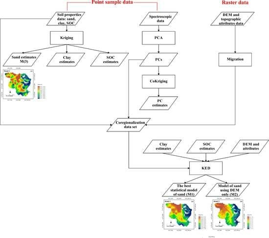
2.7. Mapping Methods Comparison

The comparison between KED and ordinary kriging (OK) was carried out in cross-validation using the two statistics suggested by Carroll and Cressie [63]: the mean error (ME) and the root mean squared standardized error by standard deviation of kriging (RMSSE):
M E = 1 n α = 1 n z * ( x α ) z ( x α )
R M S S E = α = 1 n [ z * ( x α ) z ( x α ) ] 2 σ 2 ( x α ) n
where z * ( x α ) is the estimated value at location x, z ( x α ) the measured value at the same location, and σ ( x α ) is the standard deviation of kriging (OK or KED) at the same location (x). ME was used to assess the unbiasedness of the estimation, and its optimal value should be about zero; RMSSE was used to assess estimation accuracy, and its optimal value should be about 1.
For the comparison, the correlation coefficient between observation and estimation as well as the one between standardized error and estimation were also calculated.

3. Results

3.1. Exploratory Data Analysis

The basic statistics of the soil attributes and elevation measured at 135 points are reported in Table 1. As can be seen, sand, silt, and clay exhibit sufficiently symmetrical distributions, while SOC shows a great positive asymmetry. Therefore, it was decided to transform SOC through a Gaussian anamorphosis function before interpolating it with ordinary kriging.
Regarding the diffuse reflectance spectra measurements, in Table 2, the results of principal components analysis (PCA) are reported. Only the principal components (eigenvectors) with an eigenvalue greater than 1 are reported in Table 2. It is important to note that the first PC explains more than 85%, due to the high correlation among the reflectance at the different bands, while the second explains only less than 10% of the total variance. Since each of the remaining four PCs explains just or less than 2% of the total variance, only the first two PCs were retained, which cumulatively explain almost 95%, in order to simplify the subsequent analyses and facilitate the interpretation of the radiometric indices.
The composition of the first two rotated PCs can be derived from Figure 2.
Practically, all bands (410–1760 nm) from the visible (Vis, 380–760 nm) to the near infrared (NIR, 760–1500 nm) and part of the short-wave infrared (SWIR, 1500–3000 nm), except for a narrow range centered on about the 1400 nm band, weigh positively and significantly on PC1 (Figure 3). This can then be interpreted as an indicator of the average diffuse reflectance of the soil in the indicated radiometric range and of its color. Furthermore, remembering that absorbance is inversely proportional to reflectance, the PC1 can also be assumed to be an inverse indicator of iron oxide concentration [64].
On the PC2, mainly the bands from 1760 to 2500 nm weigh positively and significantly (Figure 2), comprising the major absorption bands for OC (primarily 1772 nm; 1871 nm; and to a lesser extent 660 nm; 2070 nm; 2177 nm; 2246 nm; 2351 nm; 2483 nm) and for clay (mainly 2201 nm and to a lesser extent 1877 nm; 1904 nm; 2177 nm; 2192 nm; 2220 nm; 2492 nm) [64]. The PC2 can therefore be interpreted as an inverse indicator of SOC and clay concentrations.

3.1.1. LiDAR Data

Table 3 shows the basic statistics of elevation and topographic attributes obtained from LiDAR data and calculated at the nodes of a one-meter mesh grid. As can be seen, the study area, with a maximum height difference of about 300 m, is characterized by high variability in its topography. There are some very steep areas with slopes of about 72 degrees that are practically inaccessible and where it is impossible to take soil samples. LS and SPI also show very high outliers, and there are areas with negative curvature, which indicate a concave surface, and others with positive curvature (convex surface), with a prevalence of those with negative curvature (negative skewness).
The high variability of the topographic attributes can be explained by the changing morphology of the catchment under study (Figure 1), with an increasing elevation gradient from west to east and southeast. Furthermore, the area is characterized by a dense drainage network with numerous tributaries of the mainstream that produce deep and narrow incisions.
In the scope of applying the KED to the sand content data, all auxiliary variables had to have been calculated or estimated at the nodes of the 1 m DEM. Therefore, clay, SOC, PC1, and PC2 kriging estimates were added to the topographic attributes.

3.1.2. Soil Properties Data

An isotropic model consisting of a nugget effect and an exponential model with a range of 394.5 m and therefore an effective range of about 1185 m (approximately the maximum size of the basin in direction 132° from the north) was fitted to the experimental variogram of the clay content (Figure 4a).
This denotes a great continuity in the variation of clay content, as is evident from its kriging map (Figure 5a), in which the highest contents occurred in the lowest parts, whereas the lowest ones were in the highest parts in the east and southeast.
Different is the behavior shown by SOC, which was previously transformed to a Gaussian variable as mentioned before. An isotropic model, including a nugget effect and a spherical model with a range of 137 m, was fitted to the experimental variogram of its Gaussian transform (Figure 4b).
The variability of SOC is thus characterized by less continuity than that of clay, with spatial autocorrelation over a shorter range (137 m). The implication of the above is also evident in the back-transformed map of SOC’s kriging estimates (Figure 5b). It is characterized by a pattern of numerous small areas of limited size. However, two macro-areas can still be distinguished: one above the median line (132°N) of the basin with higher values and the part south of this line with lower values.

3.1.3. Spectroscopic Data

An isotropic LMC consisting of three basic structures: a nugget effect, a spherical model with a short-range of 159 m, and a spherical model with a long-range of 716 m, was fitted to the set of direct and cross-experimental variograms of PC1 and PC2 (Figure 6).
As can be deduced from Figure 6, both in PC1 and PC2, the largest spatial component is unfortunately represented by the discontinuity at the origin of the graphs (intercept). That is called the nugget effect and results from insufficient density of sampling with large unsampled areas. It is also shown that in the cross-variogram, the model reaches zero within a distance of about 150 m (very low sill). This means that the extraction and rotation of the PCs produced not only statistical but also quite spatial independence of the two components at a relatively short distance. This is also verified by the high distance from the intrinsic correlation curve (dashed line) in the cross-variogram, which represents the maximum possible spatial correlation between the two variables [37].
Figure 7a shows the map of PC1, which has a somewhat reverse pattern to that of SOC. This is consistent with the previously given interpretation of PC1 as a sort of spatial indicator of average soil reflectivity. It is known, in fact, that soils with a higher organic matter content are generally darker and therefore less reflective [64].
Figure 7b shows the map of PC2, with a large zone of higher values in the north. Interpretation becomes more difficult here, as the area at lower elevation (Figure 1) includes both zones with higher clay concentrations (northwest corner) (less reflective) and zones (south and southeast) with low clay and organic matter concentrations (more reflective). Actually, the diffuse reflection by soil in the range 1700–2500 nm depends on the presence of other components beyond the texture and organic carbon. Furthermore, selective absorption also depends on the particular composition of the clay and organic matter [27].

3.2. Coregionalization Data Set

The correlation matrix between sand content and all variables assumed to be potential auxiliary variables is reported in Table 4. As can be seen, apart from the expected high negative correlation with clay and the smaller positive correlation with elevation, the other correlations are rather low. It was therefore decided to exclude SPI and curvature as possible auxiliary variables, but to retain SOC and TWI. The reason was to account for possible local influences of organic carbon and water content on the estimation of sand content because, generally, the different contents of sand can affect the soil moisture and the rate of decomposition and stabilization of the organic carbon [65]. On the other hand, spatial correlations might also be nonlinear and therefore not evaluated by Pearson’s correlation coefficient.

3.3. Kriging with External Drift

3.3.1. Trend Estimation

For the trend calculation, various combinations (T = 17) of internal (a linear function of x, y coordinates) and external drift (different linear combinations of the ten auxiliary variables selected) were compared. For the internal drift, it was preferred to consider only a linear function of the coordinates (deterministic-type variation), treating most of the variation in sand content related to spatial coordinates as stochastic and then describing it by the generalized covariance function. As can be seen from the examination of Table 5a, in which the various trend models are sorted according to mean rank, the best model with the lowest mean rank and also the lowest mean square error was the one consisting of a constant coefficient plus clay content as an auxiliary variable. This result, on the other hand, was quite predictable given the strong relationship between sand and clay, which are generally measured simultaneously in the laboratory. It therefore has little practical value since the main advantage of such predictive models is to use as predictors auxiliary variables that are more easily measured, at a lower cost, and thus more available than the primary interest variable. This statistically optimal model will then be used only as a reference, but the focus will be on other predictive models that use auxiliary variables other than textural ones.
The inclusion of the spectroscopic variables (f3, f4) after clay and SOC degrades the model, albeit slightly, with a lower mean error but a higher mean square error and mean rank. However, spectroscopic measurements, although easier to obtain than those of soil properties such as clay and SOC, require specific instrumentation, trained personnel, and a certain amount of measurement time. Furthermore, unless these measurements are made in proximal sensing with adapted equipment, they are rarely available in raster format. In the above results, it is surprising that the trend model with the inclusion of the first topographical attribute (elevation), although significantly correlated with sand content (Table 4), occupies the fifth position with a lower mean absolute error but a significantly higher mean square error and mean rank. The inclusion of the other topographic attributes worsened the performance of the model even further.

3.3.2. Generalized Covariance Function (GCf) Identification

With regard to the estimation of the generalized covariance function, the model that realizes the jackknife estimator closest to one is the one consisting of the nugget effect plus the linear component with a scale equal to 200 m (Table 5b). The spatially uncorrelated component is approximately one order of magnitude larger than the spatially correlated one.
Synthesizing the two previous results on trend estimation and identification of GCf, it can therefore be said that according to the KED approach, all intrinsic spatial variation is stochastic with a prevalence of the spatially uncorrelated component (nugget effect).
In consideration of the fact that measurements of texture and, in general, all soil properties are demanding of both man-hours and costs, it was decided to assess how much the statistically optimal sand model degraded by considering only topographic attributes as auxiliary variables. These are generally more available (less expensive) and at a much higher sampling density than observations of soil properties.
Eight trend models were then compared (Table 6), subsequently adding all the other seven topographic attributes (TRI, aspect, slope, LS, curvature, SPI, and TWI) as auxiliary variables to the elevation.
The best model in terms of both minimum mean rank and minimum mean square error is the one that uses elevation as the only auxiliary variable (Table 6a). This is indeed the only topographic attribute that shows a significant correlation with sand content, while the correlations with the other attributes were rather low.
As far as the generalized covariance function is concerned, it consists again of two structures: the nugget effect and the linear component with a 200-m scale (Table 6). However, there was a marked prevalence of the spatially uncorrelated component, which was about two orders of magnitude higher than the structured component. In addition, there are no relevant statistical differences with the generalized covariance model that uses only the nugget effect as the basic structure. The exclusion of clay as an auxiliary variable in the trend therefore also resulted in an increase in randomness regarding the sand estimation variance.
Assuming ordinary kriging as the univariate reference approach, an isotropic model containing three basic structures was fitted to the experimental variogram of the sand content: a nugget effect, a spherical model with a range of 150.99 m, and a spherical model with a range of 513 m (Figure 8).
The variogram model appears to be well structured, upper-bounded, and with the spatial component at the shorter range approximately twice as large as the uncorrelated spatial component and the structured component at the longer range.

3.4. Comparison among the Three Approaches

The results of the cross-validation of the three models for estimating sand content are shown in Table 7. Model 1, whose trend contains only the clay content as an auxiliary variable, is assumed to be the best reference model; Model 2, in which the trend has only the topographic attribute of elevation; and Model 3, assumed to be the univariate reference model with no auxiliary variables.
As expected, Model 1 is the best in terms of observation-estimate correlation, lowest bias, best accuracy, and lowest correlation between standardized errors and estimates (systematic error). This result was already predicted by comparing the seventeen trend models with different combinations of auxiliary variables, including both soil attributes and topographic attributes (Table 5 and Table 6). However, Table 7 allows us to assess the actual advantage obtained by supplementing the sand content observations with elevation, obtained from high spatial resolution LiDAR data, as the auxiliary variable. Model 2 compared to Model 3 has a higher observation-estimate correlation, albeit a small one, a lower bias, and a lower standardized error-estimate correlation (less systematic error).
The previous results made it possible to compare the three models from a statistical point of view, essentially in terms of smoothing effect, bias, and accuracy. The purpose is now to continue the comparison in terms of mapping or graphical restitution of the sand content estimates and their corresponding uncertainties.
Maps of the sand content estimates for the three models are shown in Figure 9.
It is firstly to be said that the three maps are coherent in displaying the main structures of spatial dependence. However, it is possible to highlight clear differences among the maps. The one for Model 1 (clay as the auxiliary variable, Figure 9a) shows a high degree of spatial continuity and mostly reproduces the inverse relationship with the clay due to the strong negative correlation between the two variables. The Model 2 map (trend with elevation as the auxiliary variable, Figure 9b), although quite similar to the previous one, shows greater short-range variability due to the finer spatial resolution of elevation compared to the sampling scale of clay. Finally, the Model 3 map (no trend, Figure 9c) shows less spatial continuity compared with the one of Model 1 and is characterized by more numerous micro-structures of limited extent, probably due to the random nature of the spatial variation of sand content and the coarse and not even sampling scheme. In Figure 10, the uncertainty of the estimates, as expressed by the standard deviation of estimation, is compared for the three models.
Being OK and KED linear interpolators, the estimation standard deviation depends on the observation arrangement and the mathematical model of the variogram for Model 3 (ordinary kriging) and of the generalized covariance for Models 1 and 2 (kriging with external drift) [35]. Consistently, the three models show the lowest values in the central part, where sampling is densest, and the highest values at the edges of the area. However, compared to Model 3 (Figure 9c), which faithfully reproduces the sampling pattern with minima at the sampling locations, Models 1 (Figure 10a) and 2 (Figure 10b) reveal more spatial continuity with a greater accentuation of short-range variability for Model 2.

4. Discussion

The analysis of different trend models of soil sand content using different types of auxiliary variables, including topographic attributes from LIDAR data, reveals a general low control of topography on the spatial distribution of the soil sand content. This is a relatively unexpected result since topography controls a variety of processes occurring in the soil, including erosive processes, which in turn influence the spatial variation of particle size composition. Indeed, the dependence of sand content on topography is evident also in the study area, but the results show that this control is not predominantly of a deterministic nature (trend).
The interpretation of that might be that the particle size composition of the soil in this catchment is essentially related to several other properties that are not explicitly indicated in the trend (stochastic component of variation).
The above could also explain the characteristics of the generalized covariance function (which models the stochastic component of variation), in which spatially uncorrelated variability prevails over linearly structured variability. This prevalence can be attributed to two main causes: (1) the co-presence of different factors of variation that are not clearly made explicit in the model; and (2) excessive coarseness of sampling, unable to detect processes occurring in the soil at a finer scale.
Another relatively unexpected result is that apart from elevation, which shows a low correlation with sand content and is the only topographic attribute included as an auxiliary variable in M2, the other attributes show non-significant correlations. Probably, that was due to the uncertainty of their estimates and the high morphological variability mostly generated by denudation processes (landslides and water erosion) that affected the site [39,66]. These processes caused a reworking and a spatial redistribution of surficial soil.
The reason for the rather modest improvement of the univariate model M3, achieved by including elevation as an auxiliary variable in M2, may be attributed to the particular contextual characteristics discussed above. However, this should not dissuade from continuing to investigate the real advantages of using high spatial resolution LiDAR data to improve the prediction of soil attributes. Soil measurements are generally expensive, and the collection of soil samples at specific locations may be difficult or even impossible, as occurred in this case due to the extremely steep slope. It is therefore extremely useful to have a reliable sand content prediction model using the plethora of topographic data available in a high-resolution DEM.
The introduction of elevation as an auxiliary variable has also resulted in the addition of a micro-variability component in the M2 map that is not visible in the M1 map, which appears more noticeably smoothed despite being the best from a purely statistical point of view. This, which might appear to be an advantage in that it reveals sand variability at a scale of 1 m, has a risk, however. The risk is that this micro-variability reproduces topography-related variation and not the real sand-related variation when the correlation between the primary and auxiliary variables is not very strong. Hence, the need to appropriately choose the variables to be taken as predictors.
Moreover, the results highlight that the choice of the auxiliary variables can have a significant impact not only on the mapping of estimation but also on its uncertainty. Even if the same main macro-spatial structures are reproduced by the various models (M1, M2, and M3), there may be appreciable local differences, and only a careful validation process can help in choosing the optimal model. Moreover, at unsampled locations, not only is the value of the variable very critical, but also the uncertainty with which that variable is known and on which the decision is based (decision-making).
Finally, it is worth underlining that the approach proposed proved to be quite flexible (including any type of spatial variable) and scalar; therefore, it could be applied at the same fine spatial resolution over an area much larger than the basin depending on the availability of LiDAR data. However, the extendibility of a model calibrated over a small area to a larger region may raise accuracy problems due to the non-stationarity of the response variable. Nevertheless, the scalability of the model and the general availability of LiDAR data outweigh the practical usefulness of Model 2.

5. Conclusions

The main objective of this work was to evaluate whether combining observations of soil properties with LiDAR-derived topographic attributes can be considered an efficient and straightforward approach for mapping soil texture (sand content) both at fine resolution and at a large spatial scale. LiDAR provides topographical knowledge of a vast area at a finer spatial resolution compared to manual measurements. It would then be desirable to be able to apply this tool for accurate estimates of soil properties at fine resolution. Various linear trend models using different auxiliary variables were compared. The best model from a strictly statistical point of view was the one that used only the clay variable as an auxiliary variable. This result was expected given the close inverse relationship between these two soil textural components. However, the practical advantage to be gained from the use of this statistically optimal model would be very little since the two textural variables are generally determined at the same time in the laboratory. Therefore, it was decided to investigate the advantage in terms of estimation accuracy resulting from the use of LiDAR. Indeed, the improvement obtained by using only LiDAR data (elevation) compared to the univariate (no trend) model of sand content was rather marginal. This might be due to the extreme variability and complexity of the morphology of the environment under study and to the sampling, which was inevitably rather coarse and unevenly distributed.
However, we believe that the terrain morphology detected by LiDAR can affect the textural components of soil and, indirectly, moisture and available nutrients, which play an important role in forest dynamics and growth rates. The high-resolution maps of soil properties can in turn be used by forest managers for site-specific management by delineating areas that need treatment and thus can be used in precision forestry. These practices are highly sustainable because they use fewer resources, which has implications for climate change and the economy.
It is widely recognized that LiDAR elevation data are now becoming the new standard for the production of high-resolution DEMs worldwide, which should lead to the development of new and novel methods of soil property prediction. With the increased availability of data, an improvement in digital soil mapping (DSM) can also be achieved with the application of machine learning (ML) techniques to the development of trend models, leaving geostatistics to assess and model the stochastic component of spatial variation. Anyway, ML models [39] should be not just more accurate but also less of a black box, so that important scientific insights can be extracted from soil data and such models can serve as an effective source of information and knowledge.

Author Contributions

A.C. performed geostatistical analysis, interpreted the data, and wrote the paper; G.B. conceived and designed the experiments and soil sampling, analyzed and interpreted the data, designed the figures, and wrote the paper; M.C. carried out the spectroscopic analyses and cared the geological and pedological characterization of the site, the interpretation of the data and results, and contributed to write the paper; M.M. carried out the characterization of the forest, performed the analysis and interpretation of the LiDAR data and results, and contributed to write the paper; F.V.M. mainly carried out recording and analysis of the LiDAR data, and contributed to write the paper; G.S.M. conceived and designed the experiments, discussed the results, and contributed to write the paper. All authors have read and agreed to the published version of the manuscript.

Funding

This research was funded by the project “ALForLab” PON03PE_00024_1, co-funded by the National Operational Programme for Research and Competitiveness (PON R&C) 2007–2013, through the European Regional Development Fund (ERDF) and national resources (Revolving Fund—Cohesion Action Plan (CAP) MIUR).

Data Availability Statement

The data presented in this study are available on request.

Acknowledgments

The authors thank the reviewers of this paper for providing constructive comments, which have contributed to the improvement of the published version.

Conflicts of Interest

The authors declare no conflict of interest.

References

  1. Silvero, N.E.Q.; Demattê, J.A.M.; Minasny, B.; Rosin, N.A.; Nascimento, J.G.; Rodríguez Albarracín, H.S.; Bellinaso, H.; Gómez, A.M.R. Sensing Technologies for Characterizing and Monitoring Soil Functions: A Review. Adv. Agron. 2023, 177, 125–168. [Google Scholar]
  2. Ciampalini, R.; Follain, S.; Cheviron, B.; Le Bissonnais, Y.; Couturier, A.; Moussa, R.; Walter, C. Local Sensitivity Analysis of the LandSoil Erosion Model Applied to a Virtual Catchment. In Sensitivity Analysis in Earth Observation Modelling; Elsevier: Amsterdam, The Netherlands, 2017; pp. 55–73. [Google Scholar]
  3. Yost, J.L.; Hartemink, A.E. Chapter Four—Soil Organic Carbon in Sandy Soils: A Review. In Advances in Agronomy; Sparks, D.L., Ed.; Academic Press: Cambridge, MA, USA, 2019; Volume 158, pp. 217–310. [Google Scholar]
  4. Thomas, D.S.G. 11.18 Aeolian Paleoenvironments of Desert Landscapes. In Treatise on Geomorphology; Shroder, J.F., Ed.; Academic Press: San Diego, CA, USA, 2013; pp. 356–374. ISBN 978-0-08-088522-3. [Google Scholar]
  5. McBratney, A.B.; Minasny, B.; Whelan, B. Defining Proximal Soil Sensing. In Proceedings of the Second Global Workshop on Proximal Soil Sensing, Montreal, QC, Canada, 15–18 May 2011; Adamchuk, V.I., Viscarra Rossel, R.A., Eds.; McGill University: Montreal, QC, Canada, 2011; pp. 144–146. [Google Scholar]
  6. Viscarra Rossel, R.A.; Adamchuk, V.I.; Sudduth, K.A.; McKenzie, N.J.; Lobsey, C. Proximal Soil Sensing. An Effective Approach for Soil Measurements in Space and Time. Adv. Agron. 2011, 113, 237–282. [Google Scholar] [CrossRef]
  7. Mouazen, A.M.; Alexandridis, T.; Buddenbaum, H.; Cohen, Y.; Moshou, D.; Mulla, D.; Nawar, S.; Sudduth, K.A. Monitoring. In Agricultural Internet of Things and Decision Support for Precision Smart Farming; Castrignanò, A., Buttafuoco, G., Khosla, R., Mouazen, A., Moshou, D., Naud, O., Eds.; Elsevier: London, UK, 2020; pp. 35–138. ISBN 978-0-12-818373-1. [Google Scholar]
  8. Castrignanò, A.; Buttafuoco, G. Data Processing. In Agricultural Internet of Things and Decision Support for Precision Smart Farming; Castrignanò, A., Buttafuoco, G., Khosla, R., Mouazen, A., Moshou, D., Naud, O., Eds.; Elsevier Academic Press: London, UK, 2020; pp. 139–182. ISBN 9780128183731. [Google Scholar]
  9. Deutsch, C.V. A Review of Geostatistical Approaches to Data Fusion. In Geophysical Monograph Series; American Geophysical Union (AGU): Washington, DC, USA, 2007; Volume 171, pp. 7–18. ISBN 9781118666463. [Google Scholar]
  10. Nguyen, H.; Cressie, N.; Braverman, A. Spatial Statistical Data Fusion for Remote Sensing Applications. J. Am. Stat. Assoc. 2012, 107, 1004–1018. [Google Scholar] [CrossRef]
  11. Pickett, S.; Kolasa, J.; Jones, C. Ecological Understanding. The Nature of Theory and the Theory of Nature, 2nd ed.; Academic Press: New York, NY, USA, 2010; ISBN 9780125545228. [Google Scholar]
  12. Carpenter, S.R.; Armbrust, E.V.; Arzberger, P.W.; Chapin, F.S.; Elser, J.J.; Hackett, E.J.; Ives, A.R.; Kareiva, P.M.; Leibold, M.A.; Lundberg, P.; et al. Accelerate Synthesis in Ecology and Environmental Sciences. Bioscience 2009, 59, 699–701. [Google Scholar] [CrossRef]
  13. Peters, D.P.C. Accessible Ecology: Synthesis of the Long, Deep, and Broad. Trends Ecol. Evol. 2010, 25, 592–601. [Google Scholar] [CrossRef] [PubMed]
  14. Prince, A.; Franssen, J.; Lapierre, J.-F.; Maranger, R. High-Resolution Broad-Scale Mapping of Soil Parent Material Using Object-Based Image Analysis (OBIA) of LiDAR Elevation Data. Catena 2020, 188, 104422. [Google Scholar] [CrossRef]
  15. Banwart, S.A.; Nikolaidis, N.P.; Zhu, Y.-G.; Peacock, C.L.; Sparks, D.L. Soil Functions: Connecting Earth’s Critical Zone. Annu. Rev. Earth Planet. Sci. 2019, 47, 333–359. [Google Scholar] [CrossRef]
  16. Gillin, C.P.; Bailey, S.W.; McGuire, K.J.; Gannon, J.P. Mapping of Hydropedologic Spatial Patterns in a Steep Headwater Catchment. Soil Sci. Soc. Am. J. 2015, 79, 440–453. [Google Scholar] [CrossRef]
  17. Grebby, S.; Field, E.; Tansey, K. Evaluating the Use of an Object-Based Approach to Lithological Mapping in Vegetated Terrain. Remote Sens. 2016, 8, 843. [Google Scholar] [CrossRef]
  18. Soares, M.F.; Timm, L.C.; Siqueira, T.M.; dos Santos, R.C.V.; Reichardt, K. Assessing the Spatial Variability of Saturated Soil Hydraulic Conductivity at the Watershed Scale Using the Sequential Gaussian Co-Simulation Method. Catena 2023, 221, 106756. [Google Scholar] [CrossRef]
  19. Räsänen, A.; Virtanen, T. Data and Resolution Requirements in Mapping Vegetation in Spatially Heterogeneous Landscapes. Remote Sens. Environ. 2019, 230, 111207. [Google Scholar] [CrossRef]
  20. Maesano, M.; Santopuoli, G.; Moresi, F.; Matteucci, G.; Lasserre, B.; Scarascia Mugnozza, G. Above Ground Biomass Estimation from UAV High Resolution RGB Images and LiDAR Data in a Pine Forest in Southern Italy. IForest 2022, 15, 451–457. [Google Scholar] [CrossRef]
  21. Mendonça, R.L.; Paz, A.R.d. LiDAR Data for Topographical and River Drainage Characterization: Capabilities and Shortcomings. RBRH 2022, 27, e42. [Google Scholar]
  22. Debnath, S.; Paul, M.; Debnath, T. Applications of LiDAR in Agriculture and Future Research Directions. J. Imaging 2023, 9, 57. [Google Scholar] [CrossRef]
  23. Tarolli, P. High-Resolution Topography for Understanding Earth Surface Processes: Opportunities and Challenges. Geomorphology 2014, 216, 295–312. [Google Scholar] [CrossRef]
  24. Leempoel, K.; Parisod, C.; Geiser, C.; Daprà, L.; Vittoz, P.; Joost, S. Very High-resolution Digital Elevation Models: Are Multi-scale Derived Variables Ecologically Relevant? Methods Ecol. Evol. 2015, 6, 1373–1383. [Google Scholar] [CrossRef]
  25. Curcio, A.C.; Peralta, G.; Aranda, M.; Barbero, L. Evaluating the Performance of High Spatial Resolution UAV-Photogrammetry and UAV-LiDAR for Salt Marshes: The Cádiz Bay Study Case. Remote Sens. 2022, 14, 3582. [Google Scholar] [CrossRef]
  26. Riefolo, C.; Castrignanò, A.; Colombo, C.; Conforti, M.; Ruggieri, S.; Vitti, C.; Buttafuoco, G. Investigation of Soil Surface Organic and Inorganic Carbon Contents in a Low-Intensity Farming System Using Laboratory Visible and near-Infrared Spectroscopy. Arch. Agron. Soil Sci. 2020, 66, 1436–1448. [Google Scholar] [CrossRef]
  27. Demattê, J.; Morgan, C.; Chabrillat, S.; Rizzo, R.; Franceschini, M.; da Silva Terra, F.; Vasques, G.; Wetterlind, J. Spectral Sensing from Ground to Space in Soil Science: State of the Art, Applications, Potential, and Perspectives. In Land Resources Monitoring, Modeling, and Mapping with Remote Sensing; Thenkabail, P.S., Ed.; CRC Press: Boca Raton, FL, USA, 2015; pp. 661–732. ISBN 9780429089442. [Google Scholar]
  28. Viscarra Rossel, R.A.; Walvoort, D.J.J.; McBratney, A.B.; Janik, L.J.; Skjemstad, J.O. Visible, near Infrared, Mid Infrared or Combined Diffuse Reflectance Spectroscopy for Simultaneous Assessment of Various Soil Properties. Geoderma 2006, 131, 59–75. [Google Scholar] [CrossRef]
  29. Gozukara, G.; Zhang, Y.; Hartemink, A.E. Using PXRF and Vis-NIR Spectra for Predicting Properties of Soils Developed in Loess. Pedosphere 2022, 32, 602–615. [Google Scholar] [CrossRef]
  30. Minasny, B.; McBratney, A.B. Digital Soil Mapping: A Brief History and Some Lessons. Geoderma 2016, 264, 301–311. [Google Scholar] [CrossRef]
  31. Arrouays, D.; McBratney, A.; Bouma, J.; Libohova, Z.; Richer-de-Forges, A.C.; Morgan, C.L.S.; Roudier, P.; Poggio, L.; Mulder, V.L. Impressions of Digital Soil Maps: The Good, the Not so Good, and Making Them Ever Better. Geoderma Reg. 2020, 20, e00255. [Google Scholar] [CrossRef]
  32. Chen, S.; Arrouays, D.; Leatitia Mulder, V.; Poggio, L.; Minasny, B.; Roudier, P.; Libohova, Z.; Lagacherie, P.; Shi, Z.; Hannam, J.; et al. Digital Mapping of GlobalSoilMap Soil Properties at a Broad Scale: A Review. Geoderma 2022, 409, 115567. [Google Scholar] [CrossRef]
  33. Burrough, P.A. Principles of Geographical Information Systems for Land Resources Assessment; Oxford University Press: Oxford, UK, 1986; ISBN 0198545630. [Google Scholar]
  34. Matheron, G. The Theory of Regionalized Variables and Its Applications; Ecole Nationale Superieure des Mines de Paris: Paris, France, 1971; Volume 5. [Google Scholar]
  35. Chilès, J.-P.; Delfiner, P. Geostatistics: Modeling Spatial Uncertainty, 2nd ed.; Wiley Series in Probability and Statistics; John Wiley & Sons, Inc.: Hoboken, NJ, USA, 2012; ISBN 9781118136188. [Google Scholar]
  36. Wadoux, A.M.J.C.; Román-Dobarco, M.; McBratney, A.B. Perspectives on Data-Driven Soil Research. Eur. J. Soil Sci. 2020, 72, 1675–1689. [Google Scholar] [CrossRef]
  37. Wackernagel, H. Multivariate Geostatistics: An Introduction with Applications; Springer: Berlin/Heidelberg, Germany, 2003; ISBN 3540441425. [Google Scholar]
  38. Hudson, G.; Wackernagel, H. Mapping Temperature Using Kriging with External Drift: Theory and an Example from Scotland. Int. J. Climatol. 1994, 14, 77–91. [Google Scholar] [CrossRef]
  39. Moresi, F.V.; Maesano, M.; Collalti, A.; Sidle, R.C.; Matteucci, G.; Scarascia Mugnozza, G. Mapping Landslide Prediction through a GIS-Based Model: A Case Study in a Catchment in Southern Italy. Geosciences 2020, 10, 309. [Google Scholar] [CrossRef]
  40. Buttafuoco, G.; Castrignanò, A. Study of the Spatio-Temporal Variation of Soil Moisture under Forest Using Intrinsic Random Functions of Order k. Geoderma 2005, 128, 208–220. [Google Scholar] [CrossRef]
  41. Conforti, M.; Buttafuoco, G. Insights into the Effects of Study Area Size and Soil Sampling Density in the Prediction of Soil Organic Carbon by Vis-NIR Diffuse Reflectance Spectroscopy in Two Forest Areas. Land 2023, 12, 44. [Google Scholar] [CrossRef]
  42. ARSSA. Carta Dei Suoli Della Regione Calabria—Scala 1:250000. In Monografia Divulgativa; Servizio Agropedologia; Agenzia Regionale per Lo Sviluppo e per i Servizi in Agricoltura: Soveria Mannelli, Italy, 2003. [Google Scholar]
  43. Soil Survey Staff. Keys to Soil Taxonomy, 12th ed.; USDA-Natural Resources Conservation Service: Washington, DC, USA, 2014.
  44. Olaya, V. A Gentle Introduction to SAGA GIS; The SAGA User Group Ev: Gottingen, Germany, 2004; Volume 208. [Google Scholar]
  45. Wilson, J.P.; Gallant, J.C. Terrain Analysis: Principles and Applications; John Wiley & Sons, Inc.: New York, NY, USA, 2000; ISBN 978-0-471-32188-0. [Google Scholar]
  46. Florinsky, I.V. Digital Terrain Analysis in Soil Science and Geology, 2nd ed.; Academic Press Inc.: Cambridge, MA, USA, 2016; ISBN 9780128046326. [Google Scholar]
  47. Sidari, M.; Ronzello, G.; Vecchio, G.; Muscolo, A. Influence of Slope Aspects on Soil Chemical and Biochemical Properties in a Pinus Laricio Forest Ecosystem of Aspromonte (Southern Italy). Eur. J. Soil Biol. 2008, 44, 364–372. [Google Scholar] [CrossRef]
  48. Conforti, M.; Longobucco, T.; Scarciglia, F.; Niceforo, G.; Matteucci, G.; Buttafuoco, G. Interplay between Soil Formation and Geomorphic Processes along a Soil Catena in a Mediterranean Mountain Landscape: An Integrated Pedological and Geophysical Approach. Environ. Earth Sci. 2020, 79, 59. [Google Scholar] [CrossRef]
  49. Conforti, M.; Lucà, F.; Scarciglia, F.; Matteucci, G.; Buttafuoco, G. Soil Carbon Stock in Relation to Soil Properties and Landscape Position in a Forest Ecosystem of Southern Italy (Calabria Region). Catena 2016, 144, 23–33. [Google Scholar] [CrossRef]
  50. Renard, K.G.; Foster, G.R.; Weesies, G.A.; McCool, D.K.; Yoder, D.C. Predicting Soil Erosion by Water: A Guide to Conservation Planning with the Revised Universal Soil Loss Equation (RUSLE); Agriculture Handbook No. 703; US Department of Agriculture: Washington, DC, USA, 1997; ISBN 0160489385.
  51. Moore, I.D.; Gessler, P.E.; Nielsen, G.A.; Peterson, G.A. Soil Attribute Prediction Using Terrain Analysis. Soil Sci. Soc. Am. J. 1993, 57, 443–452. [Google Scholar] [CrossRef]
  52. Sequi, P.; De Nobili, M. Determinazione Del Carbonio Organico. In Metodi di Analisi Chimica del Suolo; Violante, P., Ed.; Franco Angeli: Roma, Italy, 2000; pp. 18–25. [Google Scholar]
  53. Soil Science Division Staff. Soil Survey Manual. USDA Handbook 18; Ditzler, C., Scheffe, K., Monger, H.C., Eds.; Government Printing Office: Washington, DC, USA, 2017.
  54. Rock, B.N.; Williams, D.L.; Moss, D.M.; Lauten, G.N.; Kim, M. High-Spectral Resolution Field and Laboratory Optical Reflectance Measurements of Red Spruce and Eastern Hemlock Needles and Branches. Remote Sens. Environ. 1994, 47, 176–189. [Google Scholar] [CrossRef]
  55. Shepherd, K.D.; Walsh, M.G. Development of Reflectance Spectral Libraries for Characterization of Soil Properties. Soil Sci. Soc. Am. J. 2002, 66, 988. [Google Scholar] [CrossRef]
  56. Castrignanò, A.; Quarto, R.; Venezia, A.; Buttafuoco, G. A Comparison between Mixed Support Kriging and Block Cokriging for Modelling and Combining Spatial Data with Different Support. Precis. Agric. 2019, 20, 193–213. [Google Scholar] [CrossRef]
  57. Jackson, J.E. User’s Guide to Principal Components; John Wiley & Sons: New York, NY, USA, 2003; ISBN 978-0-471-47134-9. [Google Scholar]
  58. Cattell, R.B. The Scientific Use of Factor Analysis in Behavioral and Life Sciences; Springer: Boston, MA, USA, 1978; ISBN 978-1-4684-2264-1. [Google Scholar]
  59. Yong, A.G.; Pearce, S. A Beginner’s Guide to Factor Analysis: Focusing on Exploratory Factor Analysis. Tutor Quant. Methods Psychol. 2013, 9, 79–94. [Google Scholar] [CrossRef]
  60. SAS (Statistical Analysis System). Software Package Version 9.2; SAS Institute Inc.: Cary, NC, USA, 2017. [Google Scholar]
  61. Webster, R.; Oliver, M.A. Geostatistics for Environmental Scientists; Statistics in Practice; John Wiley & Sons, Ltd.: Chichester, UK, 2007; ISBN 9780470517277. [Google Scholar]
  62. Matheron, G. The Intrinsic Random Functions and Their Applications. Adv. Appl. Probab. 1973, 5, 439–468. [Google Scholar] [CrossRef]
  63. Carroll, S.S.; Cressie, N. A Comparison of Geostatistical Methodologies Used to Estimate Snow Water Equivalent. J. Am. Water Resour. Assoc. 1996, 32, 267–278. [Google Scholar] [CrossRef]
  64. Heege, H.J. Sensing of Natural Soil Properties. In Precision in Crop Farming: Site Specific Concepts and Sensing Methods: Applications and Results; Heege, H.J., Ed.; Springer: Dordrecht, The Netherlands, 2013; pp. 51–102. ISBN 978-94-007-6760-7. [Google Scholar]
  65. Telles, E.d.C.C.; de Camargo, P.B.; Martinelli, L.A.; Trumbore, S.E.; da Costa, E.S.; Santos, J.; Higuchi, N.; Oliveira, R.C. Influence of Soil Texture on Carbon Dynamics and Storage Potential in Tropical Forest Soils of Amazonia. Glob. Biogeochem. Cycles 2003, 17, 1040. [Google Scholar] [CrossRef]
  66. Lucà, F.; Robustelli, G.; Conforti, M.; Fabbricatore, D. Geomorphological Map of the Crotone Province (Calabria, South Italy). J. Maps 2011, 7, 375–390. [Google Scholar] [CrossRef]
Figure 1. Location of the study area and soil sampling points.
Remotesensing 15 04416 g001
Figure 2. Flowchart of the proposed methodology for improving the spatial prediction of sand content.
Remotesensing 15 04416 g002
Figure 3. Pattern of loadings multiplied by 100 of the first two principal components with values above 68.73 (black dotted line). The number 68.73 is the root mean square of all the values multiplied by 100 in the matrix of PC loadings.
Remotesensing 15 04416 g003
Figure 4. Experimental variograms (filled circle) and the fitted models (solid red line) for clay (a) and soil organic carbon (SOC) (b) concentrations. Experimental variances (horizontal dashed lines) are also shown. The symbol G before the SOC stands for Gaussian-transformed data.
Remotesensing 15 04416 g004
Figure 5. Maps of clay (a) and soil organic carbon (b) concentrations obtained with univariate ordinary kriging. The white areas within the maps are outcropping rocks.
Remotesensing 15 04416 g005
Figure 6. Linear model of coregionalization (LMC) of PC1 and PC2. Black points are the experimental variograms; red solid lines are the fitted models; red dash-dotted lines in the cross-variogram are the hull of perfect correlation; and a black dashed line is the experimental variance.
Remotesensing 15 04416 g006
Figure 7. Maps of the (a) first (PC1) and (b) second (PC2) principal components calculated from diffuse reflectance spectra. The white areas within the maps are outcropping rocks.
Remotesensing 15 04416 g007
Figure 8. Experimental variogram (filled circle) and the fitted model (solid red line) for clay concentration. Experimental variance (horizontal dashed line) is also shown.
Remotesensing 15 04416 g008
Figure 9. Maps of the sand content estimates using the three models: (a) Model 1, in which the trend includes only the clay content as an auxiliary variable; (b) Model 2, in which the trend includes only elevation; and (c) Model 3, with no trend. The white areas within the maps are outcropping rocks.
Remotesensing 15 04416 g009
Figure 10. Maps of the standard deviation of sand estimation using the three models: (a) Model 1, in which the trend includes only the clay content as an auxiliary variable; (b) Model 2, in which the trend includes only elevation; and (c) Model 3, with no trend. The white areas within the maps are outcropping rocks.
Remotesensing 15 04416 g010
Table 1. Summary statistics for the contents of sand, silt, clay, and soil organic carbon.
StatisticsSandSiltClaySOC
Minimum (%)39.001.007.000.67
Median (%)63.0022.0015.002.38
Mean (%)62.6321.3416.032.66
Maximum (%)86.0040.0029.0011.02
Stand. Dev. (%)9.736.725.041.30
Skewness (-)−0.260.000.722.69
Kurtosis (-)2.863.013.1115.58
Table 2. Decomposition of the correlation matrix of diffuse reflectance data into principal components (PC) (only PCs with eigenvalues greater than 1 are reported).
PCEigenvalueDifferenceExplained Variance (%)Cumulative Explained Variance (%)
1186.61166.3485.2185.21
220.2715.899.2694.47
34.380.812.0096.47
43.572.051.6398.10
51.520.400.6998.79
61.120.610.5199.31
Table 3. Summary statistics for the topographic attributes.
StatisticsElevationSlopeAspectLSSPITRITWICurvature
(m)(°)(-)(-)(-)(-)(-)(-)
Minimum1020.530.00−1.000.000.000.000.00−84.37
Median1168.2622.45245.524.600.010.285.900.16
Mean1171.0223.40213.275.050.230.315.98−0.02
Maximum1340.8372.86360.00112.631131.307.2324.0389.76
Stand. Dev.65.7911.44104.173.365.740.191.654.47
Skewness (-)0.180.45−0.602.2365.101.491.74−1.61
Kurtosis (-)2.272.902.0424.176394.888.7112.4440.59
Table 4. Correlation matrix of the coregionalization data set. In bold are the significant correlation coefficients with a probability level of p < 0.001.
VariablesSandClaySOCPC1PC2ElevationSlopeAspectLSSPITRITWICurvature
Sand1
Clay−0.761
SOC−0.080.021
PC1−0.050.07−0.591
PC2−0.190.28−0.13−0.041
Elevation0.42−0.370.26−0.36−0.181
Slope−0.170.080.10−0.190.03−0.171
Aspect0.18−0.10−0.01−0.06−0.040.200.051
LS−0.150.050.00−0.18−0.03−0.140.850.041
SPI−0.040.06−0.060.07−0.09−0.06−0.13−0.160.041
TRI−0.190.090.10−0.160.14−0.230.890.010.75−0.081
TWI−0.020.02−0.210.11−0.170.11−0.48−0.13−0.080.60−0.431
Curvature−0.080.210.08−0.050.300.02−0.060.07−0.33−0.25−0.07−0.371
Table 5. Automatic structure identification. T stands for trial; x, y: coordinates. For identifying the external drift, different linear combinations (T1 to T17) of the selected ten auxiliary variables were used: f1. clay; f2. SOC; f3. PC1; f4. PC2; f5. elevation; f6. slope; f7. aspect; f8. LS; f9. TRI; f10. TWI.
(a) Identification of the Order k
Mean ErrorMean Squared ErrorMean Rank
TrialRing 1Ring 2TotalRing 1Ring 2TotalRing 1Ring 2Total
T1: 1 f10.260−0.645−0.19744.02049.22046.6407.0436.9246.983
T7: 1 f1 f20.256−0.654−0.20347.21051.99049.6207.1377.1277.132
T9: 1 f1 f2 f30.529−0.676−0.07955.44058.05056.7607.9337.5747.752
T11: 1 f1 f2 f3 f40.576−0.601−0.01861.68063.08062.3808.3098.0528.179
T12: 1 f1 f2 f3 f4 f50.382−0.632−0.12964.53069.02066.7908.3598.0548.205
T2: 1 x y f10.600−1.021−0.21748.78065.71057.3207.3018.2657.787
T8: 1 x y f1 f20.745−0.934−0.10252.06067.75059.9707.5688.3927.983
T10: 1 x y f1 f2 f30.770−0.889−0.06764.92074.87069.9408.4188.5718.495
T13: 1 f1 f2 f3 f4 f5 f60.734−1.036−0.15877.28080.66078.9908.9678.7548.860
T14: 1 f1 f2 f3 f4 f5 f6 f70.884−0.888−0.00986.14096.73091.4809.4669.2449.354
T15: 1 f1 f2 f3 f4 f5 f6 f7 f80.748−0.871−0.068102.200103.600102.9009.9179.5769.745
T16: 1 f1 f2 f3 f4 f5 f6 f7 f8 f91.008−0.7830.105136.400121.700129.00010.3289.6639.993
T3: 1 f20.769−1.257−0.253108.500115.700112.10010.10410.13710.121
T17: 1 f1 f2 f3 f4 f5 f6 f7 f8 f9 f101.588−0.8740.347204.800163.000183.70011.02910.18810.605
T5: 1 f31.118−0.7350.184112.900119.100116.00010.29710.47610.387
T4: 1 x y f21.408−1.1370.125116.400163.900140.30010.51010.92210.717
T6: 1 x y f31.518−0.5310.485117.900158.400138.30010.31611.08010.701
Count of measures: Ring 1 = 1260; Ring 2 = 1281; Total = 2541 Average Neighborhood Radius: 386.57 m
(b) Covariance Identification
S1 = Nugget effect; S2 = Order 1 Generalized Covariance (G.C.), Scale = 200 m
Explained/Theorical Variance Ratios Generalized covariance
Mean square error (Q)Ring 1Ring 2RingsJackknife test S1S2
0.7010.9591.0070.9840.98532.3805.021
0.7030.9231.0400.9830.98341.3500.000
0.7171.0260.8310.9100.8940.00025.150
Table 6. Automatic structure identification. T stands for trial. For identifying the external drift, different linear combinations (T1 to T8) of topographic attributes as auxiliary variables were used: f1. elevation; f2. TRI; f3. Aspect; f4. Slope; f5. LS; f6. Curvature; f7. SPI; f8. TWI.
(a) Identification of the Order k
Mean ErrorMean Squared ErrorMean Rank
TrialRing 1Ring 2TotalRing 1Ring 2TotalRing 1Ring 2Total
T1: 1 f10.525−0.1880.16589.660100.50095.15089.660100.50095.150
T2: 1 f1 f20.8730.1370.501109.100113.500111.300109.100113.500111.300
T3: 1 f1 f2 f30.7910.0080.395116.000115.900116.000116.000115.900116.000
T4: 1 f1 f2 f3 f40.710−0.0110.345163.300142.300152.700163.300142.300152.700
T5: 1 f1 f2 f3 f4 f50.7490.0800.410155.400141.700148.500155.400141.700148.500
T6: 1 f1 f2 f3 f4 f5 f60.7700.0300.396132.700126.800129.700132.700126.800129.700
T7: 1 f1 f2 f3 f4 f5 f6 f70.4210.1730.295176.500163.200169.800176.500163.200169.800
T8: 1 f1 f2 f3 f4 f5 f6 f7 f80.1790.0800.129204.400186.800195.500204.400186.800195.500
Count of measures: Ring 1 = 3271; Ring 2 = 3343; Total = 6614 Average Neighborhood Radius: 493.06 m
(b) Covariance Identification
S1 = Nugget effect; S2 = Order 1 Generalized Covariance (G.C.), Scale = 200 m; S3 = Spline G.C., Scale = 200 m; S4 = Order 3 G.C., Scale = 200 m
Explained/Theorical Variance Ratios Generalized covariance
Mean square error (Q)Ring 1Ring 2RingsJackknife testS1S2S3S4
0.6290.9891.0141.0021.00382.4700.8260.0000.000
0.6290.9871.0161.0021.00384.1200.0000.0000.000
0.6770.9560.8210.8790.8700.00047.9800.0000.000
Table 7. Results of the cross-validation test for the three models: (1) The trend includes only the clay content as an auxiliary variable; (2) the trend includes only elevation; and (3) there is no trend. RMSSE is the root mean squared standardized error by standard deviation of kriging; r is the correlation coefficient between observation and estimation; ρ is the correlation coefficient between standardized error and estimation.
ModelMean ErrorRMSSErρ
1−0.02150.970.780.02
20.02520.900.380.02
3−0.13981.130.350.16
Disclaimer/Publisher’s Note: The statements, opinions and data contained in all publications are solely those of the individual author(s) and contributor(s) and not of MDPI and/or the editor(s). MDPI and/or the editor(s) disclaim responsibility for any injury to people or property resulting from any ideas, methods, instructions or products referred to in the content.

