


Sentinel-1 Response to Canopy Moisture in Mediterranean Forests before and after Fire Events


Abstract
:
1. Introduction
2. Materials and Methods
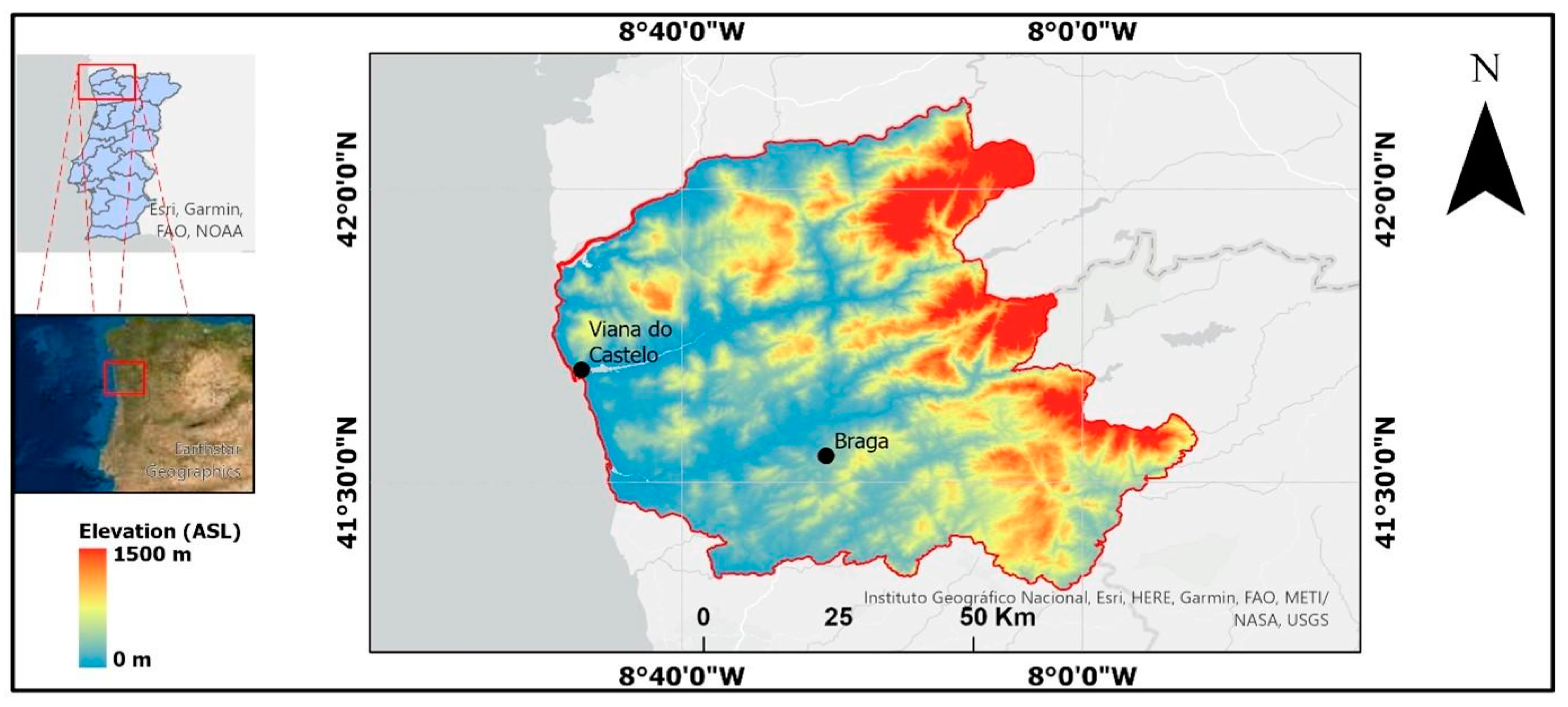
2.1. Study Area
2.2. SAR Imagery
2.3. Fire Maps
2.4. Tree Cover Map
2.5. Drought Code Map
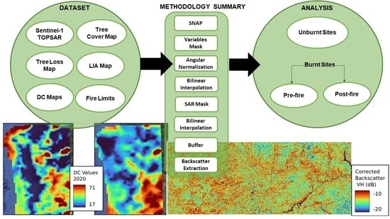
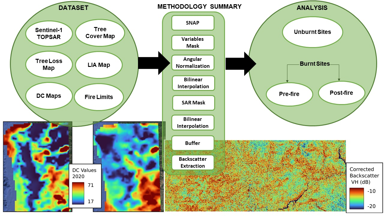
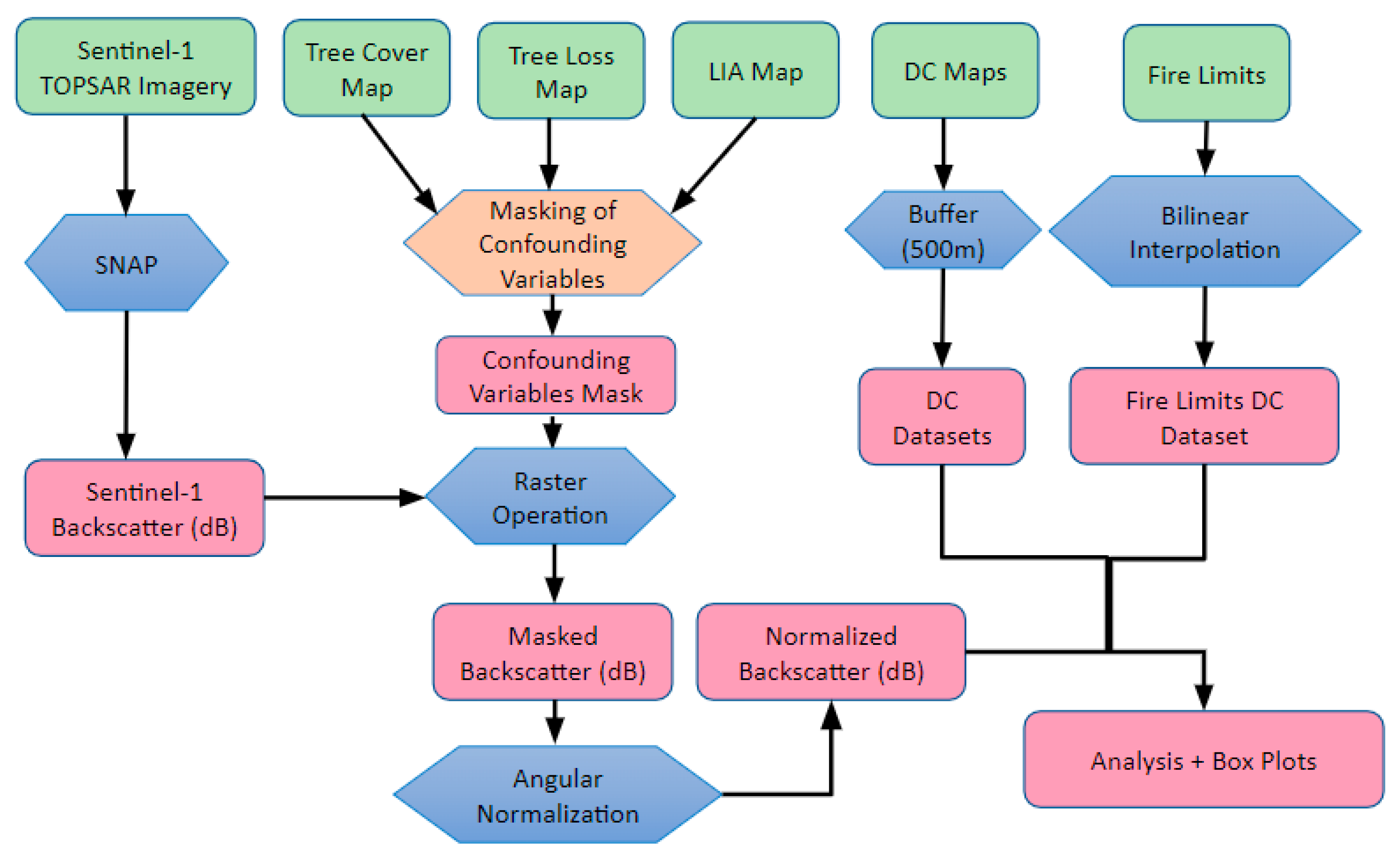
2.6. Data Processing

2.6.1. Local Incidence Angle Masking
2.6.2. Tree Cover Masking
2.6.3. Forest Loss Masking
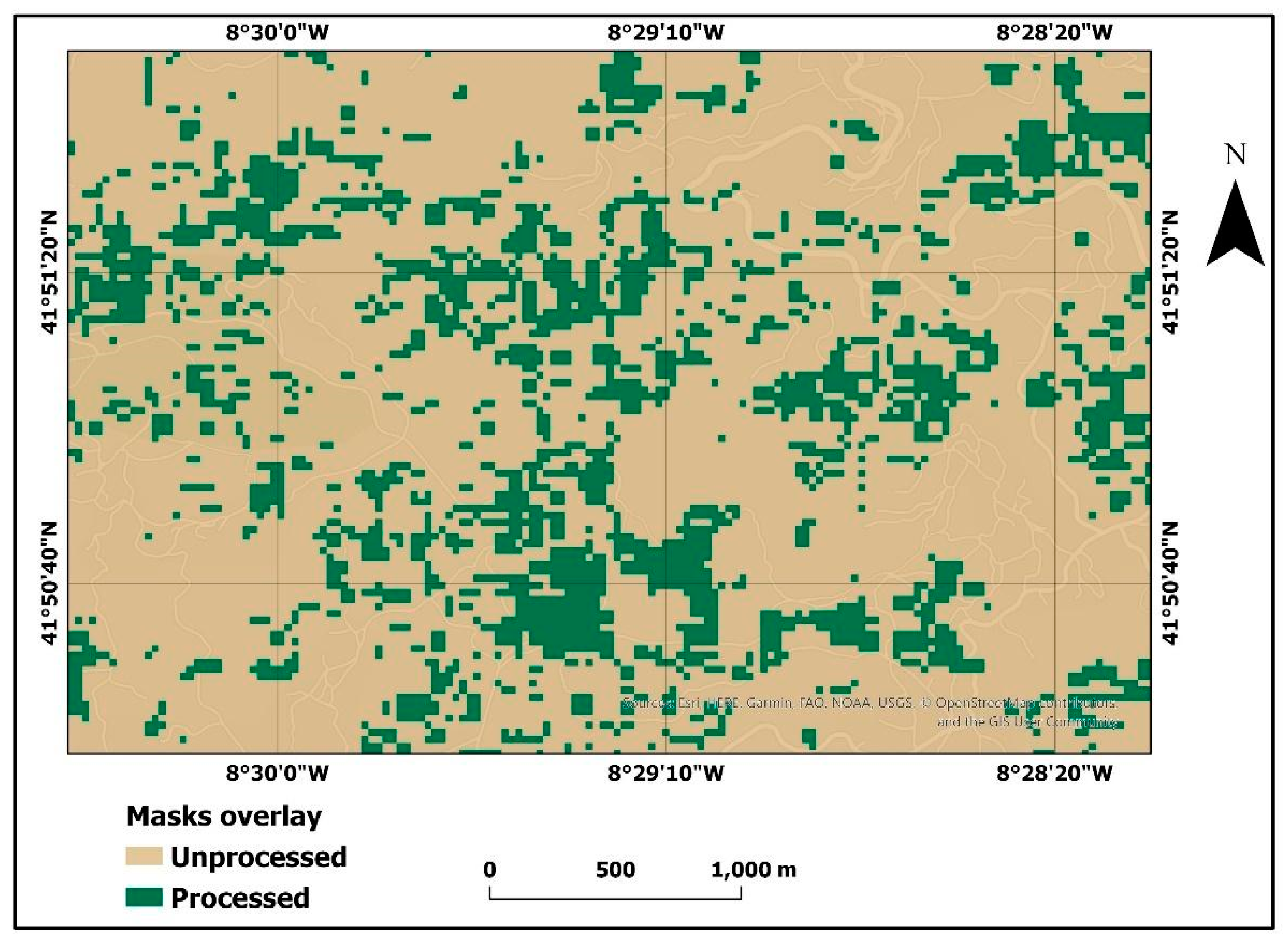
2.6.4. Cumulative Mask
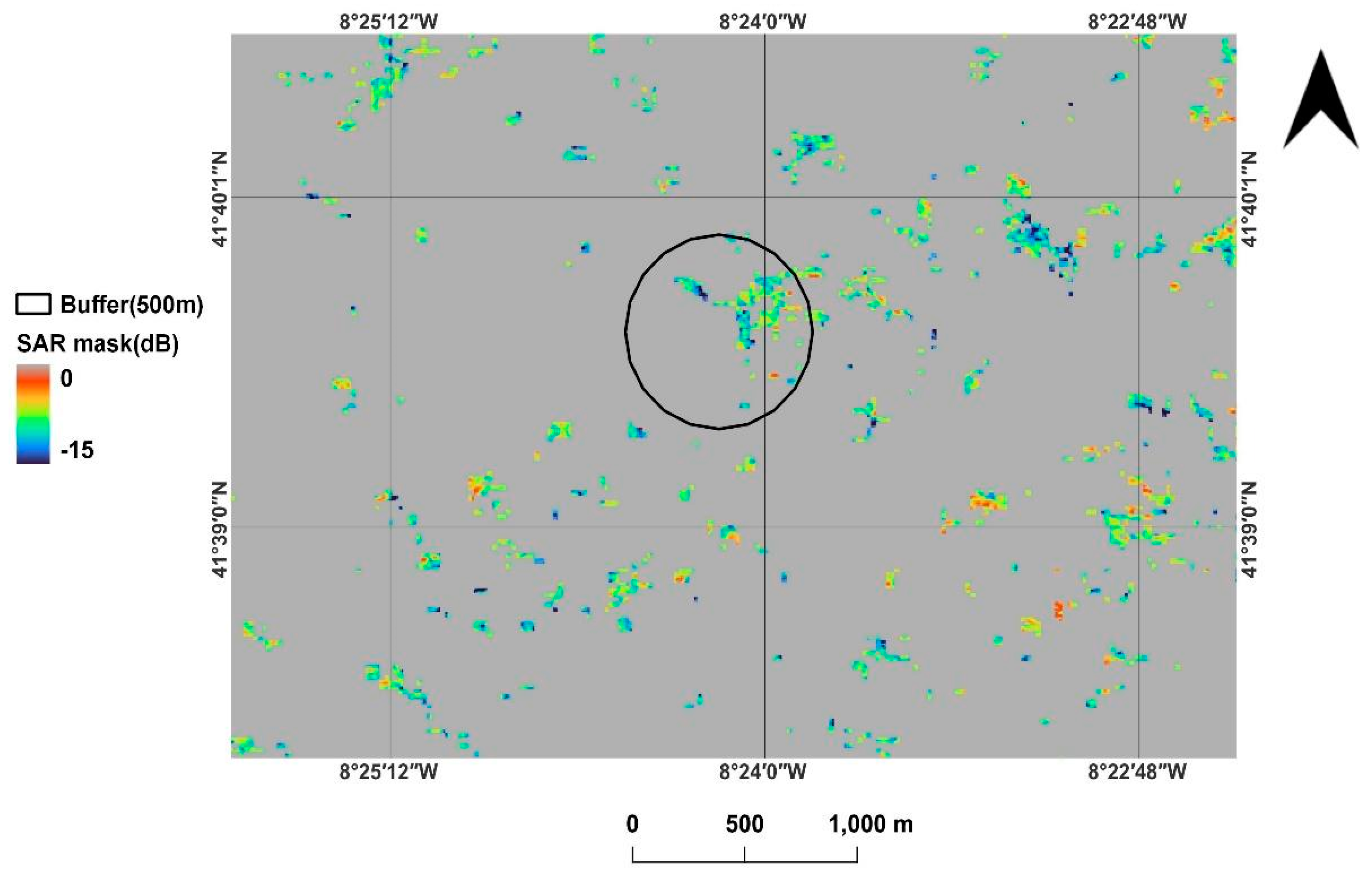
2.6.5. Backscatter Values Extraction
3. Results
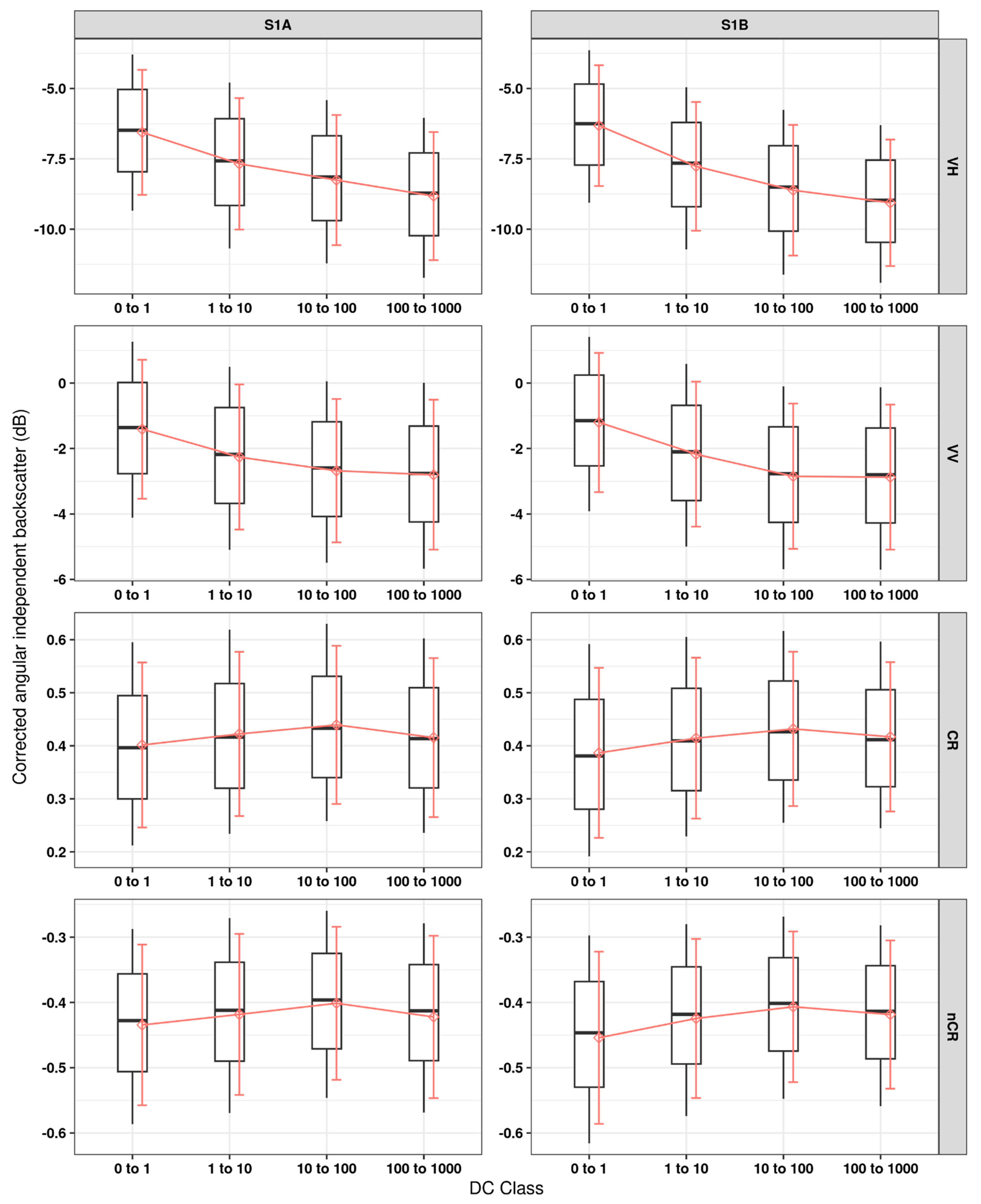
3.1. Unburnt Areas

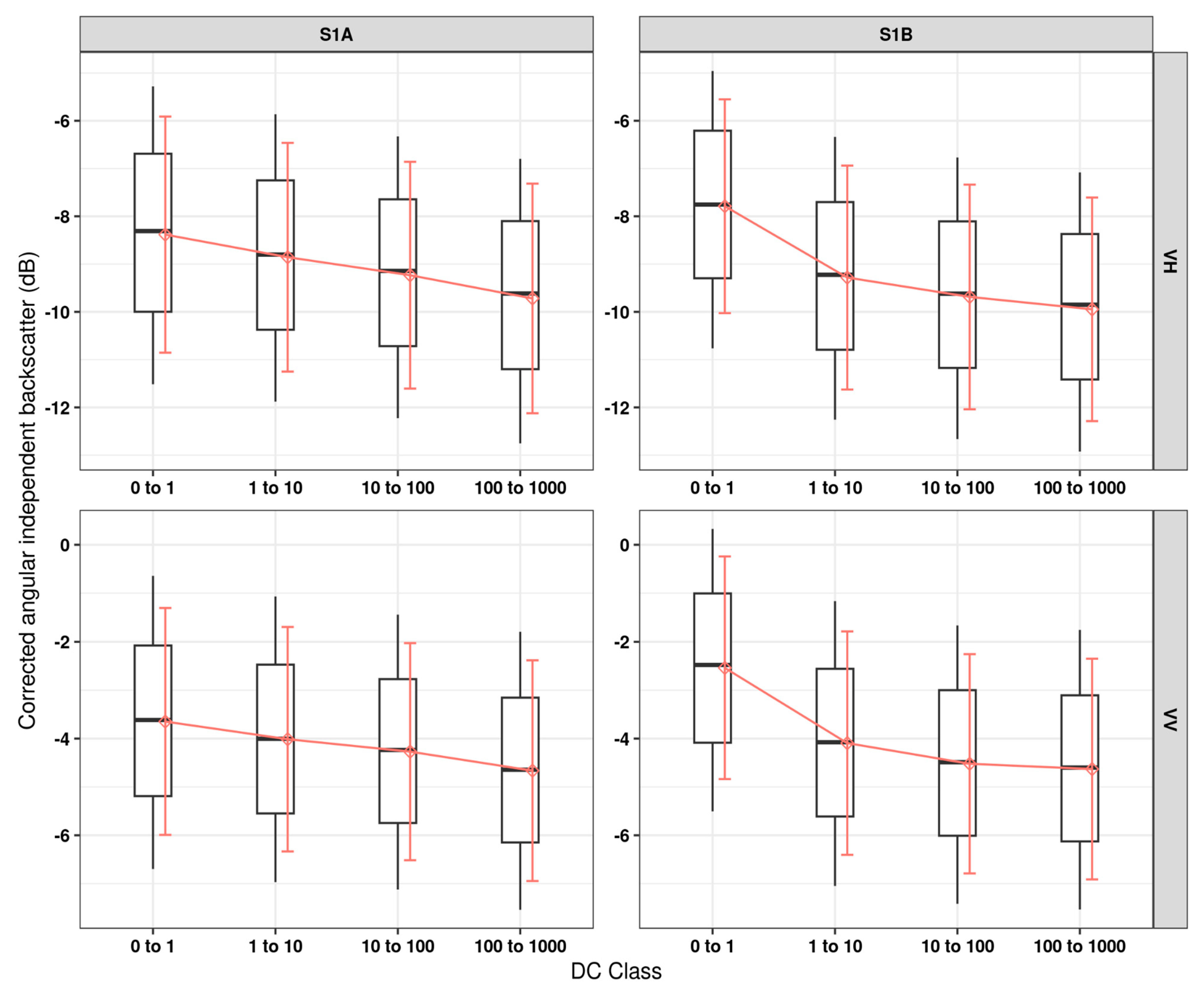
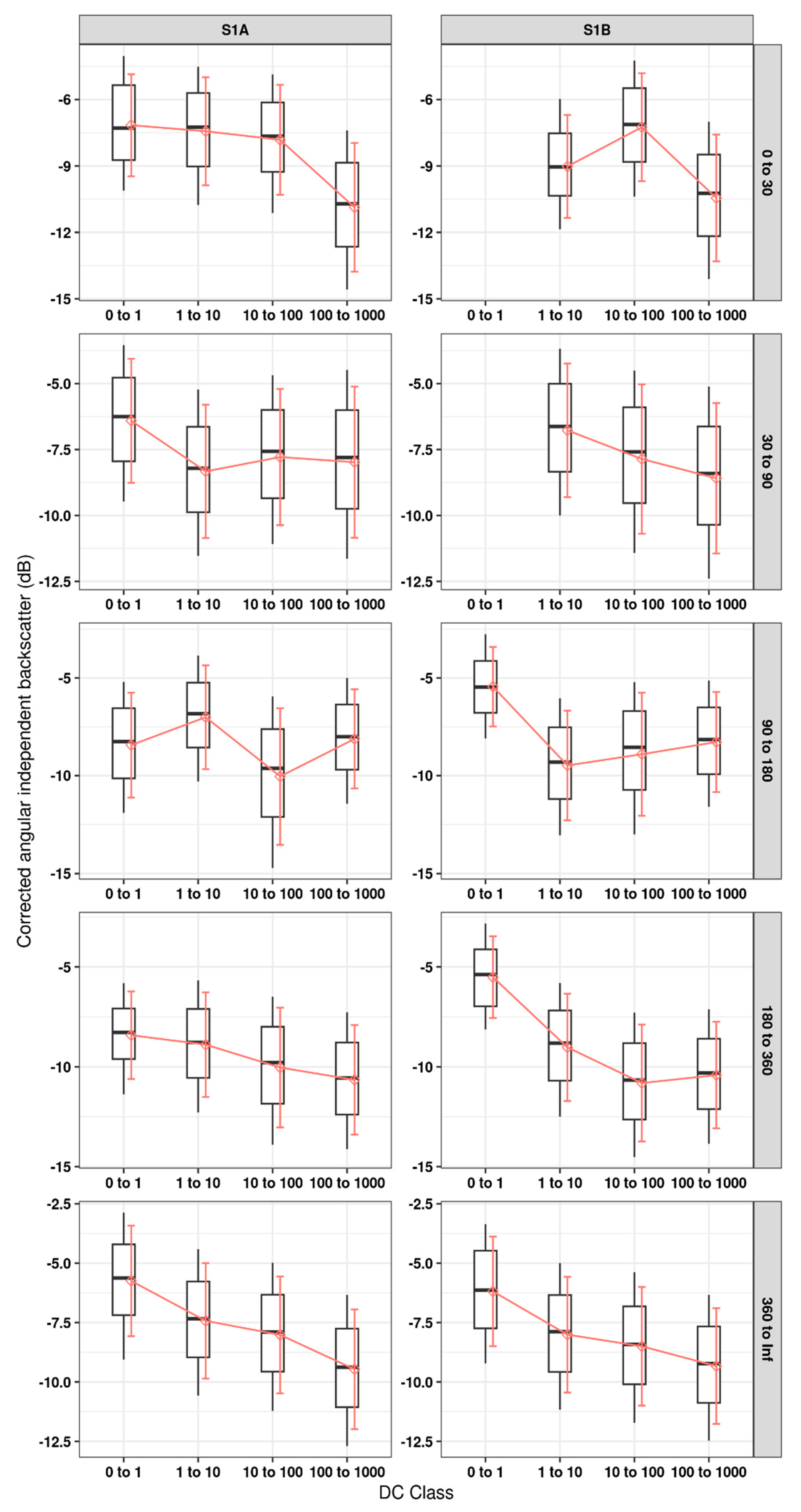
3.2. Burnt Areas
4. Discussion
5. Conclusions
Author Contributions
Funding
Data Availability Statement
Acknowledgments
Conflicts of Interest
References
- Pinto, M.M.; DaCamara, C.C.; Trigo, I.F.; Trigo, R.M.; Turkman, K.F. Fire danger rating over Mediterranean Europe based on fire radiative power derived from Meteosat. Nat. Hazards Earth Syst. Sci. 2018, 18, 515–529. [Google Scholar] [CrossRef]
- Pyne, S.J. Eternal Flame: An Introduction to the Fire History of the Mediterranean. In Earth Observation of Wildland Fires in Mediterranean Ecosystems; Springer: Berlin/Heidelberg, Germany, 2009; pp. 11–26. [Google Scholar]
- Gonçalves, A.C.; Sousa, A.M.O. The Fire in the Mediterranean Region: A Case Study of Forest Fires in Portugal. Mediterranean Identities—Environment, Society, Culture; InTech: London, UK, 2017; p. 311. [Google Scholar]
- Van Wagner, C. Development and Structure of the Canadian Forest Fire Weather Index System; Forestry Technical Report, N°35; Canadian Forestry Service: Petawawa, ON, Canada, 1987; p. 13. [Google Scholar]
- Wotton, B.M. Interpreting and using outputs from the Canadian Forest Fire Danger Rating System in research applications. Environ. Ecol. Stat. 2009, 2, 107–131. [Google Scholar] [CrossRef]
- Leblon, B.; Kasischke, E.; Alexander, M.; Doyle, M.; Abbott, M. Fire Danger Monitoring Using ERS-1 SAR Images in the Case of Northern Boreal Forests. Nat. Hazards 2002, 27, 231–255. [Google Scholar] [CrossRef]
- Yang, G.; Di, X. Adaptation of Canadian Forest Fire Weather Index System and Its Application. In Proceedings of the IEEE International Conference on Computer Science and Automation Engineering, Shanghai, China, 10–12 June 2011; pp. 55–58. [Google Scholar]
- Dimitrakopoulos, A.P.; Bemmerzouk, A.M.; Mitsopoulos, I.D. Evaluation of the Canadian fire weather index system in an eastern Mediterranean environment. Meteorol. Appl. 2011, 18, 83–93. [Google Scholar] [CrossRef]
- Oldford, S.; Leblon, B.; Maclean, D.; Flannigan, M. Predicting slow-drying fire weather index fuel moisture codes with NOAA-AVHRR images in Canada’s northern boreal forests. Int. J. Remote Sens. 2006, 27, 3881–3902. [Google Scholar] [CrossRef]
- Available online: https://www.ecmwf.int/sites/default/files/elibrary/2012/17412-describing-ecmwfs-forecasts-and-forecasting-system.pdf (accessed on 22 January 2022).
- Leblon, B. Monitoring Forest Fire Danger with Remote Sensing. Nat. Hazards 2005, 35, 343–359. [Google Scholar] [CrossRef]
- Rostami, A.; Shah-Hosseini, R.; Asgari, S.; Zarei, A.; Aghdami-Nia, M.; Homayouni, S. Active Fire Detection from Landsat-8 Imagery Using Deep Multiple Kernel Learning. Remote Sens. 2002, 14, 992. [Google Scholar] [CrossRef]
- Available online: https://cwfis.cfs.nrcan.gc.ca/background/summary/fwi (accessed on 22 January 2022).
- Vetrita, Y.; Prasasti, I.; Haryani, N.S.; Priyatna, M.; Rokhis Khomarudin, M. Drought and Fine Fuel Moisture Code Evaluation: An Early Warning System for Forest/Land Fire using Remote Sensing Approach. Int. J. Remote Sens. 2012, 9, 140–147. [Google Scholar] [CrossRef]
- Lee, J.-S.; Pottier, E. Polarimetric Radar Imaging: From Basics to Applications (Optical Science and Engineering); CRC Press: Boca Raton, FL, USA, 2009; pp. 5–6. [Google Scholar]
- Ruiz-Ramos, J.; Marino, A.; Boardman, C.P. Using Sentinel 1-SAR for monitoring long-term variation in burnt forest areas. In Proceedings of the International Geoscience and Remote Sensing Symposium (IGARSS), Valencia, Spain, 22–27 July 2018; pp. 4901–4904. [Google Scholar]
- Bourgeau-Chavez, L.L.; Leblon, B.; Charbonneau, F.; Buckley, J.R. Assessment of polarimetric SAR data for discrimination between wet versus dry soil moisture conditions. Int. J. Remote Sens. 2013, 34, 5709–5730. [Google Scholar] [CrossRef]
- Abbott, K.N.; Leblon, B.; Staples, G.C.; Maclean, D.A.; Alexander, M.E. Fire danger monitoring using RADARSAT-1 over northern boreal forests. Int. J. Remote Sens. 2007, 28, 1317–1338. [Google Scholar] [CrossRef]
- Bourgeau-Chavez, L.L.; Riordan, K.; Garwood, G. Monitoring Fuel Moisture and Improving the Prediction of Wildfire Potential in Boreal Alaska with Satellite C-Band Imaging Radar. In Proceedings of the IEEE International Geoscience and Remote Sensing Symposium, Boston, MA, USA, 8–11 July 2008; pp. 864–866. [Google Scholar]
- Leblon, B.; Bourgeau-Chavez, L.; San-Miguel-Ayanz, J. Use of Remote Sensing in Wildfire Management. In Sustainable Development—Authoritative and Leading Edge Content for Environmental Management, 1st ed.; Curkovic, S., Ed.; IntechOpen: London, UK, 2012; Chapter 3; p. 63. [Google Scholar]
- Torres, R.; Snoeij, P.; Geudtner, D.; Bibby, D.; Davidson, M.; Attema, E.; Potin, P.; Rommen, B.; Floury, N.; Brown, M.; et al. GMES Sentinel-1 mission. Remote Sens. Environ. 2012, 120, 9–24. [Google Scholar] [CrossRef]
- Soudani, K.; Delpierre, N.; Berveiller, D.; Hmimina, G.; Vincent, G.; Morfin, A.; Dufrêne, É. Potential of C-band Synthetic Aperture Radar Sentinel-1 time-series for the monitoring of phenological cycles in a deciduous forest. Int. J. Appl. Earth Obs. Geoinf. 2021, 12, 102505. [Google Scholar] [CrossRef]
- Sutariya, S.; Hirapara, A.; Meherbanali, M.; Tiwari, M.K.; Singh, V.; Kalubarme, M. Soil Moisture Estimation using Sentinel-1 SAR Data and Land Surface Temperature in Panchmahal District, Gujarat State. Int. J. Environ. Geoinformatics 2021, 8, 65–77. [Google Scholar] [CrossRef]
- Wang, L.; Quan, X.; He, B.; Yebra, M.; Xing, M.; Liu, X. Assessment of the Dual Polarimetric Sentinel-1A Data for Forest Fuel Moisture Content Estimation. Remote Sens. 2019, 11, 1568. [Google Scholar] [CrossRef]
- Available online: http://ecofun.fc.ul.pt/Activities/Desertification2014/docs2/SousaUva_The%20Portuguese%20National%20Forest%20Inventory.pdf (accessed on 14 January 2022).
- Kottek, M.; Grieser, J.; Beck, C.; Rudolf, B.; Rubel, F. World Map of the Köppen-Geiger climate classification updated. Meteorol. Z. 2006, 15, 259–263. [Google Scholar] [CrossRef] [PubMed]
- Available online: https://www.ipma.pt/pt/oclima/normais.clima/1981-2010/normalclimate8110.jsp (accessed on 14 January 2014).
- Pereira, M.G.; Trigo, R.M.; da Camara, C.C.; Pereira, J.M.C.; Leite, S.M. Synoptic patterns associated with large summer forest fires in Portugal. Agric. For. Meteorol. 2005, 129, 11–25. [Google Scholar] [CrossRef]
- San-Miguel-Ayanz, J.; Durrant, T.; Boca, R.; Maianti, P.; Libertá, G.; Artes Vivancos, T.; Jacome Felix Oom, D.; Branco, A.; De Rigo, D.; Ferrari, D.; et al. Forest Fires in Europe, Middle East and North Africa 2020; Publications Office of the European Union: Luxembourg, 2021; p. 70. [Google Scholar]
- Paulo, B.; Giuseppe, A.; Roberto, B.; Andrea, C.; Jan, K.; Giorgio, L.; San-Miguel-Ayanz, J.; Guido, S.; Ernst, S.; Hans-Helmut, D. Forest Fires in Europe 2006; Publications Office of the European Union: Luxembourg, 2007; p. 25. [Google Scholar]
- Schubert, A.; Miranda, N.; Geudtner, D.; Small, D. Sentinel-1A/B Combined Product Geolocation Accuracy. Remote Sens. 2017, 9, 607. [Google Scholar] [CrossRef]
- San-Miguel-Ayanz, J.; Durrant, T.; Boca, R.; Maianti, P.; Libertá, G.; Artés-Vivancos, T.; Oom, D.; Branco, A.; de Rigo, D.; Ferrari, D.; et al. Advance Report on Forest Fires in Europe, Middle East and North Africa 2021; Publications Office of the European Union: Luxembourg, 2022; p. 4. [Google Scholar]
- Enes, T.; Lousada, J.; Aranha, J.; Cerveira, A.; Alegria, C.; Fonseca, T. Size-density trajectory in regenerated maritime pine stands after fire. Forests. 2019, 10, 1057. [Google Scholar] [CrossRef]
- Hansen, M.C.; Potapov, P.V.; Moore, R.; Hancher, M.; Turubanova, S.A.; Tyukavina, A.; Thau, D.; Stehman, S.V.; Goetz, S.J.; Loveland, T.R.; et al. High-Resolution Global Maps of 21st-Century Tree cover Change. J. Sci. 2013, 342, 850–853. [Google Scholar]
- Ciobotaru, A.M.; Patel, N.; Pintilii, R.D. Tree cover loss in the Mediterranean region—An increasingly serious environmental issue. Forests 2021, 12, 1341. [Google Scholar] [CrossRef]
- Di Giuseppe, F.; Vitolo, C.; Krzeminski, C.; Barnard, C.; Maciel, C.; San-Miguel-Ayanz, J. Fire Weather Index: The skill provided by the European Centre for Medium-Range Weather Forecasts ensemble prediction. Nat. Hazards Earth Syst. Sci. 2020, 20, 2365–2378. [Google Scholar] [CrossRef]
- Turner, J.A. The Drought Code Component of the Canadian Forest Fire Behaviour System; Canadian Forestry Service Headquarters: Ottawa, ON, Canada, 1972; p. 5. [Google Scholar]
- Available online: https://effis.jrc.ec.europa.eu/about-effis/technical-background/fire-danger-forecast (accessed on 14 February 2022).
- Kaplan, G.; Fine, L.; Lukyanov, V.; Manivasagam, V.S.; Tanny, J.; Rozenstein, O. Normalizing the local incidence angle in sentinel-1 imagery to improve leaf area index, vegetation height, and crop coefficient estimations. Land 2021, 10, 680. [Google Scholar] [CrossRef]
- O’Grady, D.; Leblanc, M.; Gillieson, D. Relationship of local incidence angle with satellite radar backscatter for different surface conditions. Int. J. Appl. Earth Obs. Geoinf. 2013, 24, 42–53. [Google Scholar] [CrossRef]
- Vollrath, A.; Mullissa, A.; Reiche, J. Angular-based radiometric slope correction for Sentinel-1 on Google Earth Engine. Remote Sens. 2020, 12, 1867. [Google Scholar] [CrossRef]
- Paluba, D.; Laštovička, J.; Mouratidis, A.; Štych, P. Land cover-specific local incidence angle correction: A method for time-series analysis of forest ecosystems. Remote Sens. 2021, 13, 1743. [Google Scholar] [CrossRef]
- Huang, W.; Sun, G.; Ni, W.; Zhang, Z.; Dubayah, R. Sensitivity of multi-source SAR backscatter to changes in forest aboveground biomass. Remote Sens. 2015, 7, 9587–9609. [Google Scholar] [CrossRef]
- Mathieu, R.; Main, R.; Roy, D.P.; Naidoo, L.; Yang, H. The Effect of Surface Fire in Savannah Systems in the Kruger National Park (KNP), South Africa, on the Backscatter of C-Band Sentinel-1 Images. Fire 2019, 2, 37. [Google Scholar] [CrossRef]
- Kellndorfer, J. Using SAR Data for Mapping Deforestation and Forest Degradation. In The SAR Handbook: Comprehensive Methodologies for Forest Monitoring and Biomass Estimation; Flores-Anderson, A.I., Herndon, K.E., Thapa, R.B., Cherrington, E., Eds.; NASA: Huntsville, AL, USA, 2019; p. 68. [Google Scholar]
- Meyer, F. Spaceborne Synthetic Aperture Radar: Principles, Data Access, and Basic Processing Techniques. In The SAR Handbook: Comprehensive Methodologies for Forest Monitoring and Biomass Estimation; Flores-Anderson, A.I., Herndon, K.E., Thapa, R.B., Cherrington, E., Eds.; NASA: Huntsville, AL, USA, 2019; p. 28. [Google Scholar]
- Shorachi, M.; Kumar, V.; Steele-Dunne, S.C. Sentinel-1 SAR Backscatter Response to Agricultural Drought in The Netherlands. Remote Sens. 2022, 14, 2435. [Google Scholar] [CrossRef]
- Imperatore, P.; Azar, R.; Calo, F.; Stroppiana, D.; Brivio, P.A.; Lanari, R.; Pepe, A. Effect of the Vegetation Fire on Backscattering: An Investigation Based on Sentinel-1 Observations. IEEE J. Sel. Top. Appl. 2017, 10, 4478–4492. [Google Scholar] [CrossRef]
- Tanase, M.A.; Santoro, M.; de La Riva, J.; Pérez-Cabello, F.; le Toan, T. Sensitivity of X-, C-, and L-Band SAR Backscatter to Burn Severity in Mediterranean Pine Forests. IEEE Trans. Geosci. Remote Sens. 2010, 48, 3663. [Google Scholar] [CrossRef]
- Belenguer-Plomer, M.; Chuvieco, E.; Tanase, M. Temporal Decorrelation of C-Band Backscatter Coefficient in Mediterranean Burned Areas. Remote Sens. 2019, 11, 2661. [Google Scholar] [CrossRef] [Green Version]
- Zhou, Z.; Liu, L.; Jiang, L.; Feng, W.; Samsonov, S.V. Using long-term SAR backscatter data to monitor post-fire vegetation recovery in tundra environment. Remote Sens. 2019, 11, 2230. [Google Scholar] [CrossRef]
- Tanase, M.; de la Riva, J.; Santoro, M.; Pérez-Cabello, F.; Kasischke, E. Sensitivity of SAR data to post-fire forest regrowth in Mediterranean and boreal forests. Remote Sens. Environ. 2011, 115, 2075–2085. [Google Scholar] [CrossRef]
- Tanase, M.A.; Santoro, M.; Aponte, C.; de la Riva, J. Polarimetric Properties of Burned Forest Areas at C- and L-Band. IEEE J. Sel. Top. Appl. 2014, 7, 267–276. [Google Scholar] [CrossRef]
- Bernhard, E.-M.; Stein, E.; Twele, A.; Gähler, M. Synergistic use of optical and radar data for rapid mapping of forest fires in the European Mediterranean. ISPRS Archives. 2012, 4, 27–32. [Google Scholar] [CrossRef]
- LaRocque, A.; Phiri, C.; Leblon, B.; Pirotti, F.; Connor, K.; Hanson, A. Wetland Mapping with Landsat 8 OLI, Sentinel-1, ALOS-1 PALSAR, and LiDAR Data in Southern New Brunswick, Canada. Remote Sens. 2020, 12, 2095. [Google Scholar] [CrossRef]
- Vaglio Laurin, G.; Puletti, N.; Tattoni, C.; Ferrara, C.; Pirotti, F. Estimated Biomass Loss Caused by the Vaia Windthrow in Northern Italy: Evaluation of Active and Passive Remote Sensing Options. Remote Sens. 2021, 13, 4924. [Google Scholar] [CrossRef]


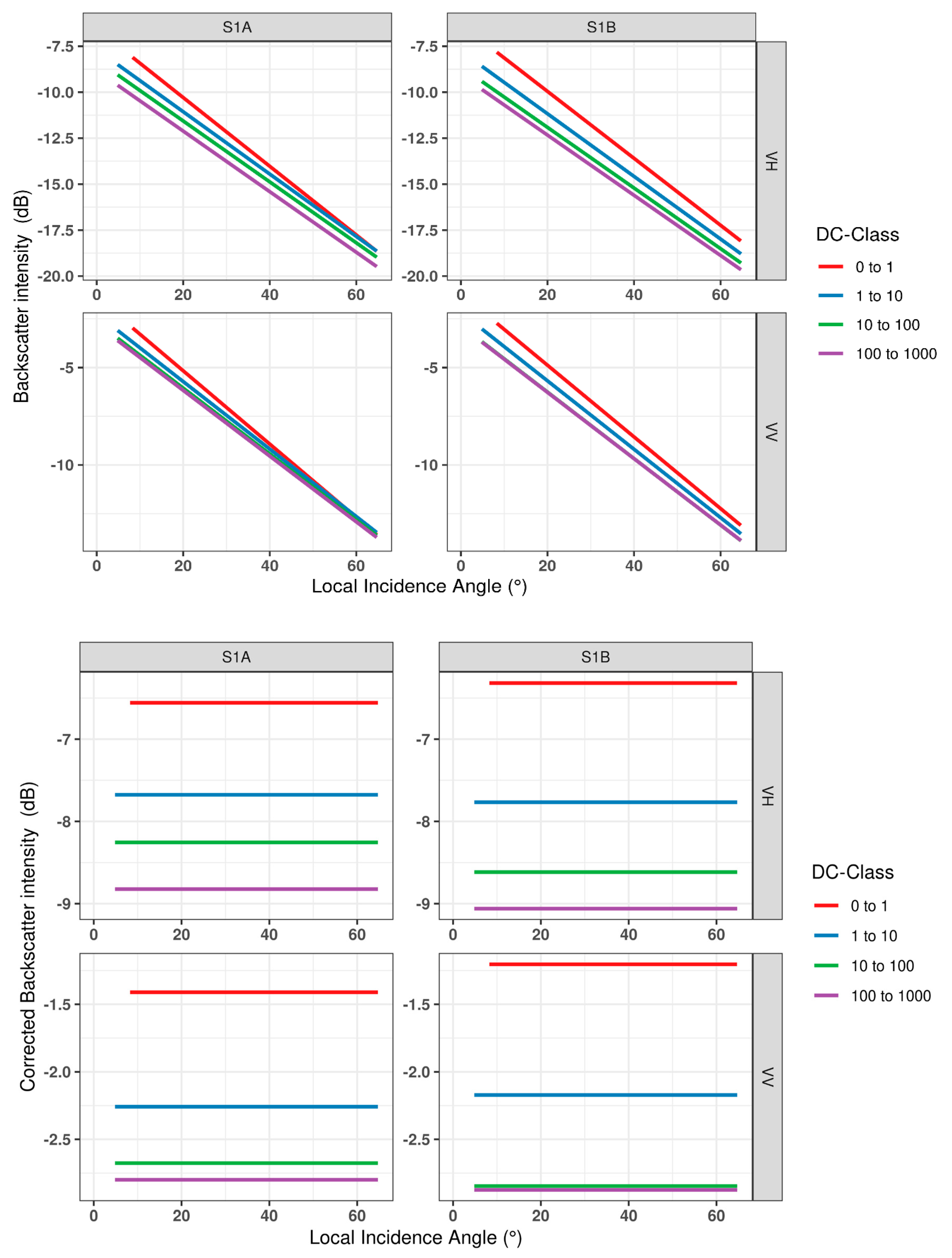
| Sensor & Pol. | _ | DC-Class | Mean (dB) | Mean DC | Linear Regression Parameters | ||
|---|---|---|---|---|---|---|---|
| Equation | R2 | N | |||||
| S1A | 0 to 1 | −13.61 | 0.58 | y = −6.20 + −0.19(x) | 0.408 | 83413 | |
| VV | 1 to 10 | −13.99 | 3.94 | y = −7.55 + −0.17(x) | 0.331 | 735476 | |
| 10 to 100 | −14.45 | 35.26 | y = −8.07 + −0.17(x) | 0.328 | 666649 | ||
| 100 to 1000 | −14.98 | 346.90 | y = −8.70 + −0.17(x) | 0.324 | 1143507 | ||
| S1B | 0 to 1 | −13.24 | 0.61 | y = −6.14 + −0.19(x) | 0.421 | 35631 | |
| VV | 1 to 10 | −14.14 | 4.48 | y = −7.60 + −0.17(x) | 0.344 | 703635 | |
| 10 to 100 | −14.77 | 35.75 | y = −8.41 + −0.17(x) | 0.326 | 772728 | ||
| 100 to 1000 | −15.16 | 343.66 | y = −8.91 + −0.17(x) | 0.329 | 1114588 | ||
| S1A | 0 to 1 | −8.51 | 0.58 | y = −0.94 + −0.20(x) | 0.438 | 83341 | |
| VH | 1 to 10 | −8.73 | 3.92 | y = −2.11 + −0.18(x) | 0.366 | 739908 | |
| 10 to 100 | −9.02 | 35.24 | y = −2.48 + −0.17(x) | 0.365 | 667006 | ||
| 100 to 1000 | −9.17 | 342.10 | y = −2.65 + −0.17(x) | 0.356 | 1117419 | ||
| S1B | 0 to 1 | −8.17 | 0.61 | y = −0.99 + −0.19(x) | 0.431 | 35537 | |
| VH | 1 to 10 | −8.76 | 4.49 | y = −1.97 + −0.18(x) | 0.377 | 702264 | |
| 10 to 100 | −9.23 | 35.75 | y = −2.63 + −0.18(x) | 0.364 | 771789 | ||
| 100 to 1000 | −9.24 | 343.68 | y = −2.70 + −0.17(x) | 0.359 | 1113898 | ||
| Polarization | Sensor | DC Class Pair | Mean Backscatter Difference. | Lower end Confidence Interval | Upper end Confidence Interval |
|---|---|---|---|---|---|
| VV | B-A | −0.85 | −0.92 | −0.78 | |
| S1A | C-B | −0.42 | −0.45 | −0.39 | |
| D-C | −0.12 | −0.15 | −0.09 | ||
| B-A | −0.97 | −1.07 | −0.86 | ||
| S1B | C-B | −0.67 | −0.70 | −0.64 | |
| D-C | −0.03 | −0.06 | 0.00 | ||
| VH | B-A | −1.12 | −1.19 | −1.04 | |
| S1A | C-B | −0.58 | −0.61 | −0.55 | |
| D-C | −0.57 | −0.60 | −0.54 | ||
| B-A | −1.45 | −1.56 | −1.34 | ||
| S1B | C-B | −0.85 | −0.88 | −0.82 | |
| D-C | −0.44 | −0.47 | −0.42 |
Disclaimer/Publisher’s Note: The statements, opinions and data contained in all publications are solely those of the individual author(s) and contributor(s) and not of MDPI and/or the editor(s). MDPI and/or the editor(s) disclaim responsibility for any injury to people or property resulting from any ideas, methods, instructions or products referred to in the content. |
© 2023 by the authors. Licensee MDPI, Basel, Switzerland. This article is an open access article distributed under the terms and conditions of the Creative Commons Attribution (CC BY) license (https://creativecommons.org/licenses/by/4.0/).
Share and Cite
Pirotti, F.; Adedipe, O.; Leblon, B. Sentinel-1 Response to Canopy Moisture in Mediterranean Forests before and after Fire Events. Remote Sens. 2023, 15, 823. https://doi.org/10.3390/rs15030823
Pirotti F, Adedipe O, Leblon B. Sentinel-1 Response to Canopy Moisture in Mediterranean Forests before and after Fire Events. Remote Sensing. 2023; 15(3):823. https://doi.org/10.3390/rs15030823
Chicago/Turabian StylePirotti, Francesco, Opeyemi Adedipe, and Brigitte Leblon. 2023. "Sentinel-1 Response to Canopy Moisture in Mediterranean Forests before and after Fire Events" Remote Sensing 15, no. 3: 823. https://doi.org/10.3390/rs15030823