Monitoring Corn Nitrogen Concentration from Radar (C-SAR), Optical, and Sensor Satellite Data Fusion

Abstract

Corn (Zea mays L.) nitrogen (N) management requires monitoring plant N concentration (Nc) with remote sensing tools to improve N use, increasing both profitability and sustainability. This work aims to predict the corn Nc during the growing cycle from Sentinel-2 and Sentinel-1 (C-SAR) sensor data fusion. Eleven experiments using five fertilizer N rates (0, 60, 120, 180, and 240 kg N ha⁻¹) were conducted in the Pampas region of Argentina. Plant samples were collected at four stages of vegetative and reproductive periods. Vegetation indices were calculated with new combinations of spectral bands, C-SAR backscatters, and sensor data fusion derived from Sentinel-1 and Sentinel-2. Predictive models of Nc with the best fit (R² = 0.91) were calibrated with spectral band combinations and sensor data fusion in six experiments. During validation of the models in five experiments, sensor data fusion predicted corn Nc with lower error (MAPE: 14%, RMSE: 0.31 %Nc) than spectral band combination (MAPE: 20%, RMSE: 0.44 %Nc). The red-edge (704, 740, 740 nm), short-wave infrared (1375 nm) bands, and VV backscatter were all necessary to monitor corn Nc. Thus, satellite remote sensing via sensor data fusion is a critical data source for predicting changes in plant N status.

1. Introduction

Nitrogen (N) is the most limiting nutrient for corn (Zea mays L.) production, with fertilization via inorganic fertilizers being one of the most relevant sources [1,2,3]. Nitrogen fertilizer requirement is estimated as the difference between soil nutrient supply and crop demand linked to the target yield [4]. This estimation is not simple, and the optimal fertilizer N rate calculation presents a significant degree of uncertainty [5], mainly linked to environmental conditions during the crop growing season. Although traditional methods can adequately estimate fertilizer N needs based on soil analysis at or right before sowing time [6,7,8,9], these methods do not consider seasonal weather conditions [10]. Therefore, improved techniques for monitoring crop N status should be explored to better inform decisions on fertilization and adjust crop N needs. The crop N nutrition index (NNI) is a diagnostic method based on the characterization of plant biomass (W) and N concentration (Nc), which allows for the identification of changes in crop N status during growing [11]. However, determining the mentioned parameters (W and Nc) is labor-intensive, time-consuming, and expensive [12]. Hence, it is necessary to explore a novel method to characterize and address this complex challenge and adapt crop N requirements more efficiently.

Remote sensing, mainly linked to the utilization of transmittance and spectral reflectance proximal sensors, has been evaluated as an appropriate option to monitor corn N status [13,14]. Proximal sensors collect information close to the crop canopy at distances of less than 100 cm, for which reflectance or transmittance sensors (chlorophyll meters) are used [15]. For the proximal reflectance sensor, a critical component of the NNI, Nc, has been modeled from the utilization of vegetation indices (based on the infrared and visible regions of the spectrum) [16]. For example, vegetation indices measured from proximal reflectance sensors such as CropCircle^TM and GreenSeeker^TM and the SPAD index from the SPAD^TM chlorophyll meter have been used to monitor N demand and adjust fertilization needs in situ [13,14,15,16,17,18]. Several investigations reported a significant level of Nc prediction from vegetation indices with red-edge bands, such as normalized difference red-edge (NDRE) and red-edge vegetation index (RERVI), determined from proximal sensors [13,14,17]. In addition, model performance has been reported to improve when using a combination of vegetation indices [13,14]. Past research [18], using the normalized difference vegetation index (NDVI) and NDRE, developed a combined vegetation index (canopy chlorophyll content index, CCCI) to predict overall within-canopy N content for wheat (Triticum aestivum L.). Additionally, the CCCI demonstrated good ability in predicting corn Nc during vegetative stages [14]. More recently, it has been reported that the simplified CCCI (SCCCI = NDRE/NDVI) successfully predicted leaf Nc [13]. However, the fundamental drawback of these sensors is their low spatial coverage since they measure close to, or in contact with, the plant, which is unsuitable for evaluating a whole field and capturing the spatial variability of Nc [19,20]. Optical sensors onboard satellites are an alternative to monitoring the crop N status, allowing the capturing of the corn’s spatio-temporal variability at the field scale.

Satellite remote sensing tools obtain information on land and water surfaces through remote observations of electromagnetic radiation reflected or emitted by the Earth’s surface [21]. Remote sensors can be classified as passive (optical) or active (radar). Passive remote sensing detects solar energy reflected and emitted by the Earth instead of that generated by a sensor. With remote optical sensors, vegetation indices have been developed to monitor biophysical parameters related to N management in corn [22,23]. Currently, remote optical sensors on Sentinel-2 satellite platforms observe the visible spectrum, red-edge, near-infrared, and short-wave infrared. The spectral (multispectral), radiometric, temporal (revisit time), and spatial resolutions are high [24]. The European Space Agency (ESA) provides observations from Sentinel-2 openly and freely. For these reasons, crop monitoring in precision agriculture with Sentinel-2 has been successful [25]. More recently, the importance of the red-edge spectrum for monitoring corn chlorophyll content from Sentinel-2 remote optical sensors has been highlighted [26]. Thus, vegetation indices combining red-edge bands from remote sensing tools can improve the current monitoring of corn Nc during its growth cycle. However, these sensors have the disadvantage of not receiving land surface information in cloudy conditions [21,27]. An alternative is found in C-band Synthetic Aperture Radar (C-SAR) systems that can relieve Earth surface information at night or during inclement weather, except in the most severe conditions [21]. Therefore, remote optical sensors could monitor corn Nc throughout its growth cycle complemented with C-SAR systems.

The C-SAR sensors emit their energy, making them independent of solar and ground radiation [21]. The C-SAR system emits a microwave (5.4 GHz) electromagnetic pulse to measure the time and intensity of the echo reflected from the Earth’s surface (backscatter) [21,28]. The C-SAR system can control the direction of the emitted electric field in horizontal (H) and vertical (V) polarizations. In addition, it can receive wave returns on both H and V channels. The C-SAR backscatters are highly sensitive to plant structural differences (stalk:leaf ratio, height, wet and dry W, and water content), while optical indices saturate during advanced corn growth stages [28,29]. The C-SAR backscatters have been used to monitor the biophysical parameters of different crops [30,31,32,33], specifically corn [34,35,36]. Radar vegetation indices with backscatters were adjusted to dry W in oilseed rape (Brassica napus L.) [37]. In addition, normalization of C-SAR backscatter to local incidence angle (LIA) has been shown to improve crop monitoring [38]. Currently, the ESA openly and freely provides active observations from the C-SAR system on the Sentinel-1 satellite platforms. The Sentinel-1 C-band synthetic aperture radar (SAR) instruments support operation in both single-polarization (HH or VV) and dual-polarization (HH+HV or VV+VH) modes, with high temporal and spatial resolutions; the exact resolution depends on the operational mode and the observation scene [21]. Therefore, Sentinel-1 and Sentinel-2 are powerful tools for monitoring growing crops. However, these sensors have yet to be calibrated for monitoring the Nc throughout the entire crop cycle.

Previous studies have focused on determining corn’s Nc through proximal sensors and monitoring other biophysical characteristics of corn through remote sensing techniques [13,14,35,39,40]. Recent research has advanced crop monitoring by utilizing red-edge bands [26] or manipulating C-SAR data from remote sensing [38]. These methods can provide valuable information for real-time monitoring of crop N status and predicting Nc during the growing season, which can aid in making informed decisions about fertilizer application. However, there is still a need to improve the estimation of Nc in corn by exploring data fusion approaches that integrate Sentinel-1 and Sentinel-2 data. This study aims to test sensor data fusion of spectral bands and C-SAR backscatters to more accurately predict the Nc of the entire corn crop cycle, which leads to more precise N fertilization management for corn and better predictions of crop N needs.

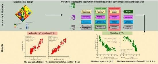
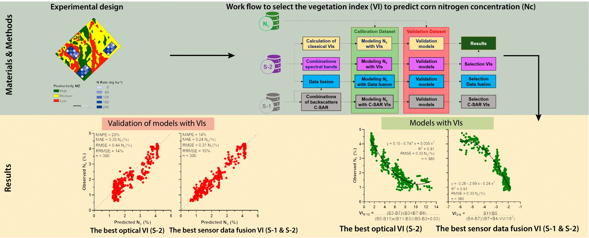
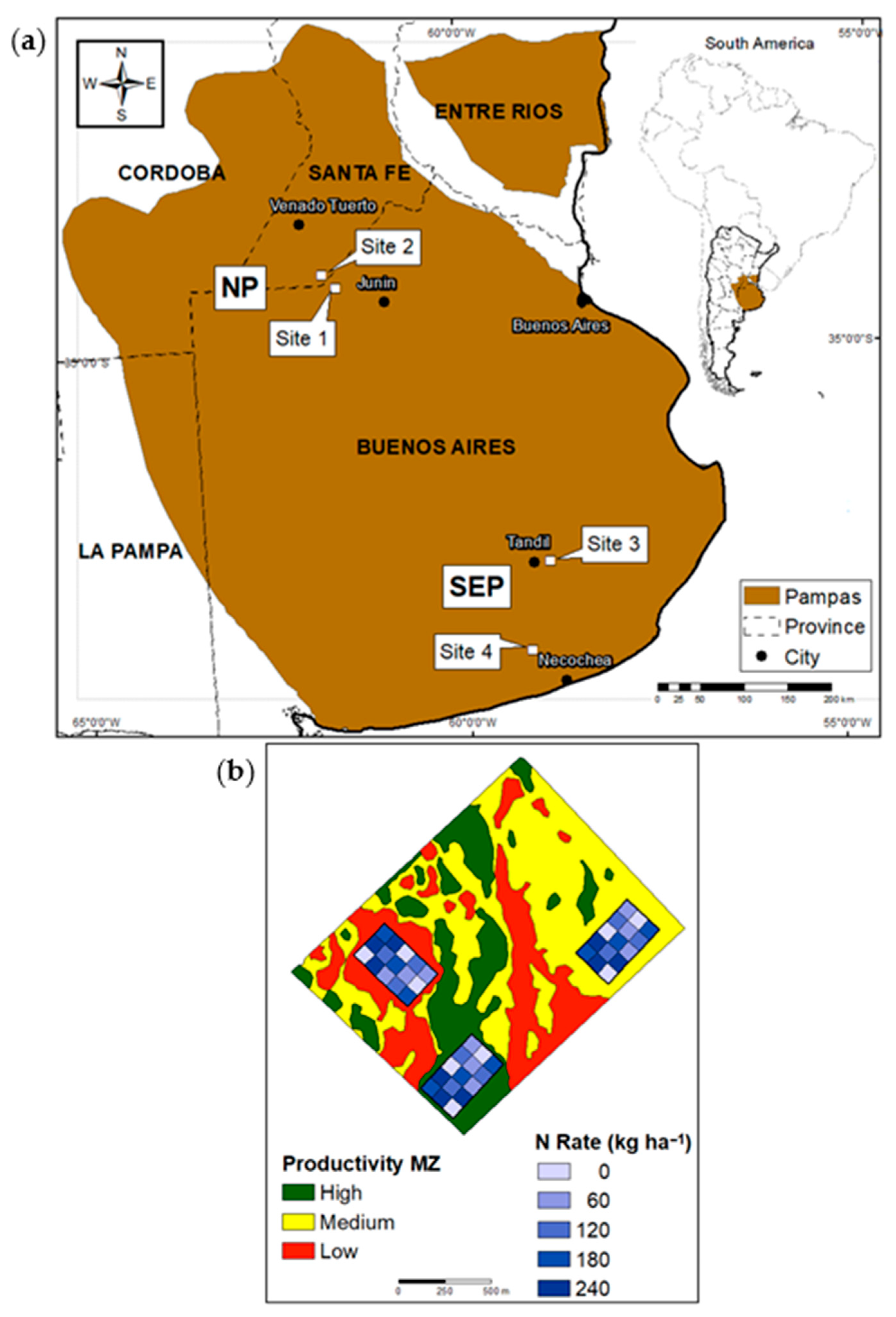
2. Materials and Methods

A conceptual framework was developed to test all options to model corn Nc from the calculation of vegetation indices (VIs), the combination of spectral bands, and the data fusion integrating these options with C-SAR backscatters for calibration and then validation datasets (Figure 1).

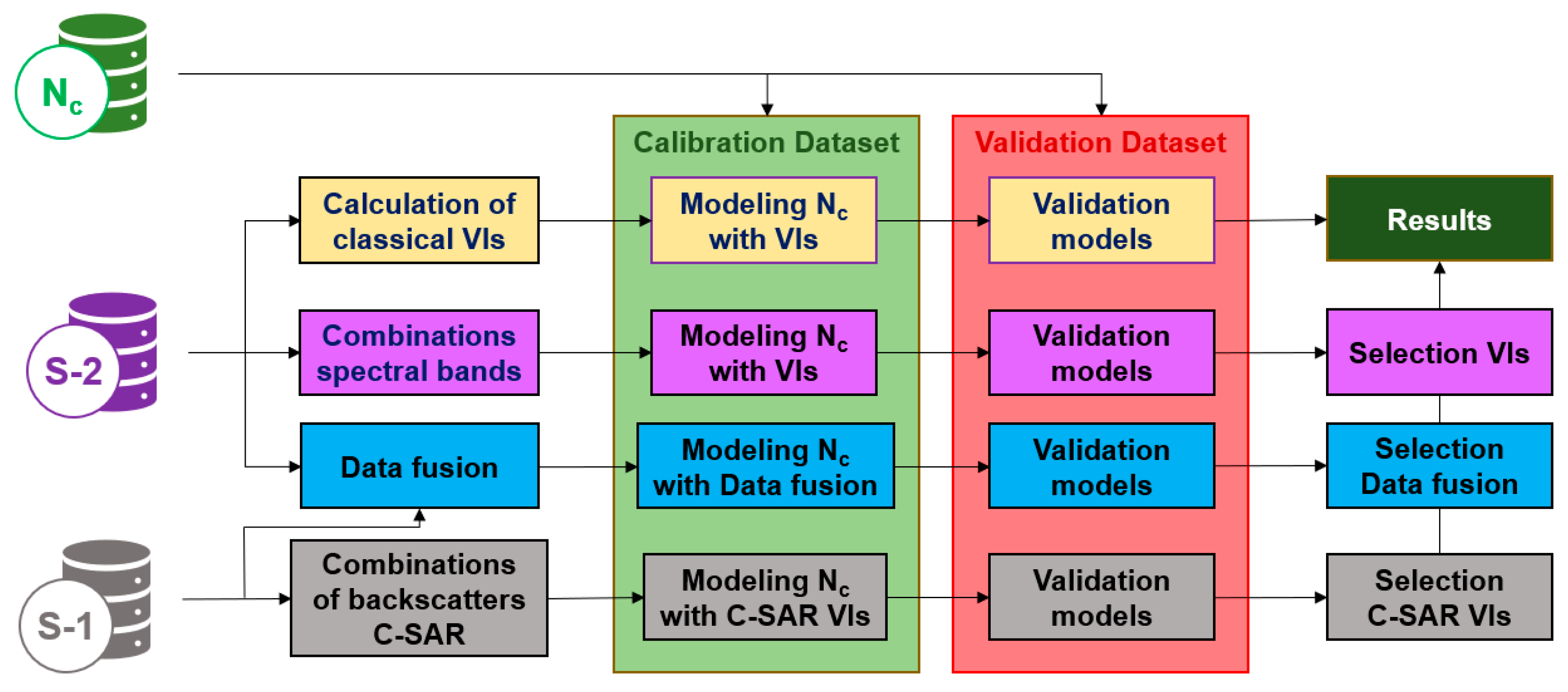
2.1. Description of Field Studies

During the 2020–2021 corn growing season, 11 field experiments were conducted on four commercial farms (sites) in the Pampas region of Argentina. The Pampas region is one of the world’s most productive areas and is characterized by deep Mollisol soils with dark horizons [41]. The sites were selected and grouped into two subregions with contrasting soil and climate conditions (

Table 1. Corn management characteristics (sowing and harvest date, plant density), soil texture, soil organic matter (SOM), and nitrate–nitrogen (NO₃⁻–N) content for 11 experiments.

Site	Exp (MZ)	Sowing Date	Harvest Date	Plant Density Plants m−2	Soil Texture (0–20 cm)	SOM (0–20 cm) g kg−1	NO3−–N (0–60 cm) kg ha−1
1	1(VH)	22 September	23 March	9.0	Sandy loam	3.8	72
	2(L)	22 September	23 March	8.0	Loamy sand	2.5	42
	3(H)	23 September	23 March	9.0	Sandy loam	3.7	70
	4(M)	23 September	23 March	8.5	Sandy loam	3.5	46
2	5(H)	24 September	23 March	8.9	Sandy loam	2.9	48
	6(L)	25 September	22 March	7.8	Loamy sand	2.2	34
	7(M)	29 September	22 March	8.3	Sandy loam	2.7	36
3	8(H)	7 November	19 May	6.7	Loam	5.9	46
	9(L)	7 November	19 May	4.7	Clay loam	5.6	40
4	10(H)	21 November	26 May	4.4	Loam	5.5	78
	11(L)	21 November	26 May	3.4	Clay loam	5.5	90

Exp: experiment number, MZ: productive management zones, VH: very high, H: high, M: medium, L: low.

and Figure 2): (i) northern Pampas (NP) (Site 1 and Site 2; sub-humid Pampa subregion; Typic Hapludoll/Typic Argiudoll soils; 975 mm mean annual precipitation; 19.2 °C mean annual air temperature) and (ii) south-eastern Pampas (SEP) (Site 3 and Site 4; humid Pampa subregion; Typic Argiudoll soils; 950 mm mean annual precipitation; 13.5 °C mean annual air temperature) [42]. Soils from the SEP present a loamy texture and a soil organic matter (SOM) concentration ranging from 50 to 60 g kg⁻¹ on the surface horizon. In contrast, the soils from the NP are characterized by a sandy loam and silty loam texture and a lower SOM concentration (20 to 30 g kg⁻¹) compared to the SEP [43].

Within each site, each experiment was located in different management zones (MZ) delimited according to historical yields of the last five years, topography according to the digital elevation model, water accumulation and slope maps, and the average and coefficient of variation of the NDVI from the last five summer crops [44] (Figure 2). The MZ determined varied from two to four depending on the site (i.e., four MZ at Site 1, three MZ at Site 2, and two MZ at Sites 3 and 4), totaling in 11 experiments.

In each experiment, the experimental design was a randomized complete block with three replications and five fertilizer N rates of 0, 60, 120, 180, and 240 kg N ha⁻¹. The N source was urea (46-0-0) applied at corn sowing. Plant density and sowing date in each field were optimal according to farmer management. Based on soil testing information, phosphorus, sulfur, potassium, and micronutrients were not limited. The experimental unit size varied between 60 × 60 and 80 × 80 m, with an area of analysis of 50 × 50 m.

In each experimental unit, plant samples were collected at ground level during corn’s sixth, tenth, and fourteenth developed leaf and flowering growth stages (V₆, V₁₀, V₁₄, and R₁, respectively, [45]) (

Table 2. Dates of sampling, satellite observations, and cumulative precipitation since planting for the 2020–2021 corn season for each experiment by stage.

Exp	Sampling Stage	Sampling Date	Satellite Observation Acquisition		Cumulative Precipitation (mm)
			Sentinel-1	Sentinel-2
1, 2, 3, and 4 (Site 1)	V6	10 and 11 November	6 and 12 November	7 and 12 November	118
	V10	3 and 4 December	30 November and 6 December	27 November and 7 December	153
	V14	21 and 22 December	18 and 24 December	17 and 22 December	194
	R1	5 and 6 January	5 January	1 January	198
5, 6, and 7 (Site 2)	V6	11 November	6 and 12 November	7 and 17 November	94
	V10	4 December	30 November and 6 December	7 and 27 November	114
	V14	20 December	18 and 24 December	17 and 22 December	114
	R1	6 January	5 January	1 January	163
8 and 9 (Site 3)	V6	14 December	14 December	14 December	25
	V10	2 January	1 January	31 December and 3 January	33
	V14	23 January	19 and 25 January	23 January	181
	R1	4 February	31 January and 6 February	4 February	181
10 and 11 (Site 4)	V6	29 and 30 December	1 January	26 and 30 December	96
	V10	22 January	19 and 25 January	20 and 23 January	182
	V14	5 February	6 February	4 February	205
	R1	20 February	18 and 24 February	22 February	306

). The sampling scheme represented pixels with 10 to 20 m spatial resolution [24]. Local sampling consisted of 12 individual plants according to the Elemental Sampling Unit (ESU) scheme of the VALERI methodology [46]. The collected plants were air-dried in an oven at 60 °C, ground, and passed through a 0.5 mm sieve for chemical analysis. The Nc in corn plants was determined by the Kjeldahl method [47].

2.2. Remote Sensing Data

In a Geographic Information System (GIS) environment, sampling point locations were digitized and represented as point entities (shapes). The data from Sentinel-1 and Sentinel-2 remote sensing observations were transferred to these entities by applying an appropriate data extraction function. Sentinel-2 observations had an average temporal resolution of five days and a spatial resolution of 10 or 20 m, depending on the spectral band. Sentinel-2 observations were obtained at Level-2A Bottom-Of-Atmosphere (BOA) reflectance. The nomenclature of the spectral bands was B2 (blue, 492 nm, 10 m), B3 (green, 559 nm, 10 m), B4 (red, 665 nm, 10 m), B5 (red-edge 1, 704 nm, 20 m), B6 (red-edge 2, 740 nm, 20 m), B7 (red-edge 3, 780 nm, 20 m), B8 (near-infrared, 833 nm, 10 m), B8A (865 nm, 20 m), B11 (short-wave infrared spectral range 1, 1375 nm, 20 m), and B12 (short-wave infrared spectral range 2, 1612 nm, 20 m).

The C-SAR backscatters (Sentinel-1) were in Ground Range Detected (GRD) and interferometric wide-swath (IW) mode. The orbit was downward with an incidence angle range of 30–45°. Preprocessing was conducted with the tools available through the ESA Sentinels Application Platform (SNAP, version: 8.0) software package as established by [48]: Apply Orbit File–Thermal Noise Removed–Removed GRD Border Noise–Radiometric Calibration–Multi-looking (4 × 4)–Speckle (Lee 3 × 3)–Range Doppler Terrain Correction. Vertical–horizontal (VH) and vertical–vertical (VV) backscatters were obtained in dB normalized by Beta Naught (β₀) and at a spatial resolution of 10 m. VH and VV backscattering values were normalized by the local angle of incidence (LIA) proposed by [38] and represented as VHxLIA and VVxLIA.

When the plant sampling dates did not correspond with the satellite observation dates, the weighted average of the energy values of the two observations closest to the sampling date was calculated. In the case of Sentinel-2, this methodology was applied to the spectral bands. For Sentinel-1, the specific methodology consisted of multiplying the local angle of incidence (LIA) by the LIA-corrected VH and VV backscatters. The result was the LIA-corrected VH and VV backscatters in SNAP, and these backscatters were multiplied by LIA, resulting in the nomenclatures VHxLIA and VVxLIA. Weighed means were calculated on the sampling date for the four variables (VH, VV, VHxLIA, and VVxLIA). The weighting was based on the number of days since the sample date.

2.2.1. Traditional Vegetation Indices

Sentinel-2 spectral bands were used to derive those traditional vegetation indices commonly used in the literature (Table S1 in Supplementary Materials). These indexes were computed over plant sample locations and at different phenological stages (V₆, V₁₀, V₁₄, and R₁).

2.2.2. Combinations of Spectral Bands and C-SAR Backscatters and Data Fusion

The 14 vegetation indices presented in

Table 3. Vegetation indices for a combination of a, b, and c.

Vegetation Index (VI)	Equation
VI1	a − b
VI2	a/b
VI3	(a − b)/(a + b)
VI4	(a − b)/(a + b + 0.25) × 1.25
VI5	(a − b)/(a + b + 0.5) × 1.5
VI6	(a − b)/(a + b + 0.75) × 1.75
VI7	(2a + 1 − (√((2a + 1)2 − 8 × (a − b)))/2
VI8	(a − b)/(a + b − c)
VI9	(a2 − b × c)/(a2 + b × c)
VI10	100 × (a − b) − 10 × (a − c)
VI11	(a − b) − 0.2 × (a − c) × (a/b)
VI12	(a − b) × (b − c)/(a − c + 0.03)
VI13	(a − b)/(a + b)/(a − c)/(a + c)
VI14	2.5 × (a − b)/(a + 6 × b − 7.5 × c) + 1
Combined	VI1-14/VI2-14 (with a, b, and c randomly assigned)

are helpful for satellite monitoring of N in corn [12,13,14,22] and are referenced in Table S1 of the Supplementary Material. Vegetation indices were calculated using spectral bands (B2, B3, B4, B5, B6, B7, B8, B8A, B11, and B12) and Sentinel-1 VH and VV backscatters, which were either corrected or not corrected by the LIA (VHxLIA and VVxLIA). The VH and VV backscatter values were in absolute decibel values divided by 100, and those of VHxLIA and VVxLIA were also in absolute values divided by 10,000. This step was necessary to standardize the VH and VV values between 0 to 1 so that they were similar to the scale of the lower-resolution spectral bands. The values of VHxLIA and VVxLIA were 1000 to 10,000 because they resulted from VH times LIA, i.e., 43 × 34. Thus, in the vegetation index equations, VH appears as VH/10² and VHxLIA as VHxLIA/10⁴. This way, backscatter values similar to those of the Sentinel-2 spectral bands were obtained.

Each spectral band and the C-SAR backscatters were evaluated as variables a, b, and c of the 14 vegetation index formulas presented in Table 3. All potential combinations of the available spectral bands and backscatters were considered while creating different vegetation indices, such as NDVI, SAVI, SR, and others. Furthermore, each vegetation index was divided by another to obtain combined vegetation indices. In this case, the divisor index formula utilized random assignment of a, b, and c as spectral bands and backscatters during each iteration.

The methodology for evaluating and selecting models is shown in Figure 3, and it employs an iterative function (loop) to process the data. The spectral bands and C-SAR backscatters were used to calculate the vegetation indices as variables a, b, and c of the formulas in Table 3. For this, a matrix (M) was entered with the type of experiment (calibration or validation), the observed variable, the spectral bands, and the C-SAR backscatters. The input data was matrix M = [Nc, B2, B3, B4, B5, B6, B7, B8, B8A, B11, B12, VH/10², VV/10², VHxLIA/10⁴, VVxLIA/10⁴, experiment]. During each iteration, three columns of M (except Nc and experiment) were assigned as variables a, b, and c, which were used to calculate the vegetation indices formulated in Table 3. Combined vegetation indices were also calculated, dividing each vegetation index by all successor formulas of its numbering in Table 3 by assigning three columns of M as the variables a, b, and c at random. For example, six combined vegetation indices were generated from VI₈ resulting from the following ratios: VI₈/VI₉, VI₈/VI₁₀, VI₈/VI₁₁, VI₈/VI₁₂, VI₈/VI₁₃, and VI₈/VI₁₄. Figures S1 and S2 of the supplementary material show detail about this process.

Continuing in the same iteration, after the individual and combined vegetation indices were calculated, they were compiled together with M in a new matrix called VIs. In the VIs matrix, the points identified with the calibration experiment id were selected. These points were assigned to a new matrix called Cal. The Cal matrix (Figure S2) fitted each vegetation index to the Nc using linear and second-degree polynomial regression models. The significance of each generated model was then evaluated by determining the p-value of the regressor parameters, specifically β₁ for linear models and both β₁ and β₂ for quadratic polynomial models. Further, each model was diagnosed according to the assumptions of linearity (“RESET”), normality (“Kolmogorov–Smirnov”), homoscedasticity (“Breusch–Pagan”), and autocorrelation (“Durbin–Watson”). When autocorrelation was significant, the iterative module “cochrane.orcutt” [49,50,51] was applied. Models that had significant β₁ and β₂ regressor parameters (p-value < 0.05) and exceeded the diagnostic assumptions were validated in the validation experiments (Figure 3).

Proceeding within the same iteration, in each of the five validation experiments, the Nc prediction error was determined according to the mean absolute percentage error (MAPE), a metric used to evaluate the predictive performance of the regressor models [52]. The MAPE values obtained from the five validation experiments were averaged to obtain the validation MAPE. The MAPE of the calibration set was also calculated. The final MAPE was calculated as the maximum value between the validation and calibration MAPE values. Each final MAPE of each vegetation index was compared to the slightest stored prediction error (e). If the final MAPE was found to be less than the e value, the value of e was updated to the current MAPE, and the VI associated with the model was recorded as the model predictor. This procedure recounted in one iteration was performed in each iteration (cycles) until all spectral bands and C-SAR backscatters were combined. Thus, by utilizing the MAPE metric, the modeled Nc was obtained from the vegetation index with the lowest prediction error at the end of the iteration process. Thus, the best vegetation indices were selected from all possible combinations of the C-SAR backscatters, spectral bands, and spectral bands with C-SAR backscatters (sensor data fusion). More details are given in Figure S2 in the supplementary material.

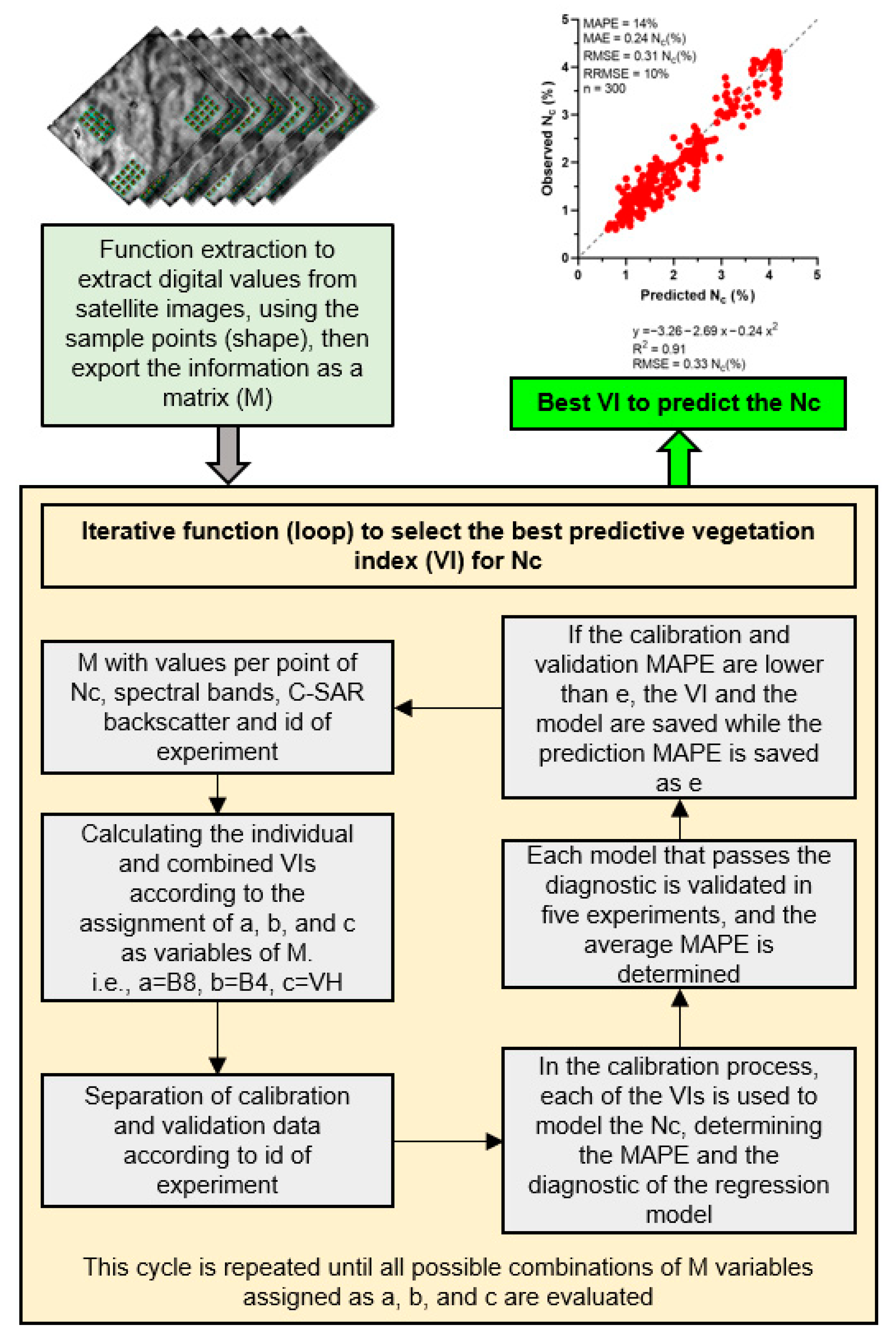
2.3. Statistical Analysis

The calibration dataset was six experiments at Sites 1 and 4. The validation dataset was five experiments at Sites 2 and 3. The Nc was modeled with the calibration dataset, and the calibrated models were validated with the validation dataset. Therefore, the statistical analysis comprised two parts; the first was to model Nc with linear and quadratic models from the vegetation indices of six experiments (Sites 1 and 4). The second was to evaluate the prediction error of the modeled Nc for data from five experiments in contrasting environments (Sites 2 and 3). The coefficient of determination (R²) and root-mean-square error (RMSE) were calculated for the calibration experiments. For each experiment’s validation, RMSE, the RMSE relative to the observed mean (RRMSE), the mean absolute error (MAE), and the MAPE were determined as statistical metrics of the prediction error. The errors of the five experiments were then averaged for each prediction error metric. The analyses were conducted using R software R version 3.6.3 (www.r-project.org, accessed on 1 July 2022).

$$\mathrm{MAPE} \left(\%\right)=\frac{1}{n} {\displaystyle \sum }_{\mathrm{i}=1}^{\mathrm{n}}\frac{\left|y_i-{\widehat{y}}_i\right|}{y_i}\times 100$$

(1)

$$\mathrm{RMSE}=\sqrt{ \frac{1}{n} {\displaystyle \sum }_{i=1}^n {\left(y_i-{\widehat{y}}_i\right)}^2}$$

(2)

$$\mathrm{RRMSE} \left(\%\right)=\frac{\mathrm{RMSE}}{y_{maximum}-y_{minimum}}\times 100$$

(3)

$$\mathrm{MAE}=\frac{1}{n} {\displaystyle \sum }_{\mathrm{i}=1}^n\left|y_i-{\widehat{y}}_i\right|$$

(4)

where $y_i$ is of observed Nc, ${\widehat{y}}_i$ is the corresponding predicted Nc, n is the number of samples, and $y_{maximum}$ and $y_{minimum}$ are the maximum and minimum observed Nc.

3. Results

From the field data collection, the Nc values were normally distributed, and the averages at V₆, V₁₀, V₁₄, and R₁ were 3.80, 2.37, 1.58, and 1.21%, respectively. At all sites, Nc increased with the N rate (

Table 4. Plant nitrogen concentration (Nc) for each nitrogen (N) rate, crop growth stage, and experiment (Exp). Each value represents the average of 3 replicates.

N Rate (kg ha−1)	Exp 1	Exp 2	Exp 3	Exp 4	Exp 5	Exp 6	Exp 7	Exp 8	Exp 9	Exp 10	Exp 11
	Nc (%)	Nc (%)	Nc (%)	Nc (%)	Nc (%)	Nc (%)	Nc (%)	Nc (%)	Nc (%)	Nc (%)	Nc (%)
	V6
0	3.76 d 1	3.42 d	3.71 c	3.70 c	3.57 b	3.64 c	3.48 b	2.95 b	3.07 b	3.26 c	3.38 b
60	4.09 c	4.17 c	4.04 b	4.19 b	3.93 a	3.98 b	3.99 b	2.98 b	3.49 a	3.11 c	3.64 a
120	4.18 bc	4.41 ab	4.23 ab	4.21 b	3.98 a	4.14 a	4.13 ab	3.26 a	3.18 b	3.54 b	3.69 a
180	4.30 ab	4.22 bc	4.32 a	4.19 b	4.08 a	3.92 b	4.28 a	2.86 ab	3.22 b	3.80 a	3.58 a
240	4.44 a	4.48 a	4.31 a	4.60 a	4.03 a	4.04 ab	4.14 ab	3.41 a	3.09 b	3.69 ab	3.66 a
	V10
0	2.04 c	2.14 d	2.21 d	2.50 d	1.54 c	1.54 c	1.59 c	2.04	2.45 a	2.01 d	1.85 b
60	2.57 b	2.36 c	2.45 c	2.99 c	2.05 b	2.09 b	2.00 b	2.08	2.08 b	2.29 c	2.00 b
120	2.55 b	2.58 b	2.62 bc	3.06 c	2.08 b	2.33 ab	2.34 a	2.05	2.44 a	2.25 c	2.29 a
180	2.89 a	2.78 b	2.69 b	3.26 b	2.24 ab	2.26 ab	2.52 a	2.12	2.43 a	2.49 b	2.24 a
240	2.82 a	2.86 a	2.90 a	3.46 a	2.33 a	2.42 a	2.37 a	2.20	2.58 a	2.72 a	2.32 a
	V14
0	1.41 c	1.34 d	1.42 c	0.82 d	0.96 c	1.20 d	1.07 d	1.21 c	1.29 d	1.05 c	0.95 c
60	1.48 c	1.65 c	1.60 c	1.62 c	1.54 a	1.53 c	1.44 c	1.57 b	1.32 cd	1.26 b	1.21 b
120	1.67 bc	1.94 b	1.94 b	1.83 b	1.34 b	1.81 ab	1.78 b	1.87 a	1.49 c	1.40 b	1.29 ab
180	1.81 ab	1.96 b	1.90 b	1.84 ab	1.73 a	1.68 bc	2.01 a	1.76 ab	1.85 b	1.41 b	1.46 a
240	1.85 a	2.25 a	2.14 a	2.03 a	1.58 a	1.93 a	1.88 ab	1.82 ab	2.08 a	1.62 a	1.33 ab
	R1
0	0.81 b	0.95 d	0.99 b	0.97 c	0.66 d	0.66 c	0.68 c	0.89 c	0.92 d	0.98 b	1.08 c
60	0.94 b	1.15 c	1.08 b	1.15 c	0.78 cd	0.87 b	0.83 c	1.12 a	1.04 cd	1.37 a	1.43 b
120	1.18 a	1.21 bc	1.38 a	1.35 b	0.86 bc	1.20 a	1.17 b	1.19 a	1.17 bc	1.43 a	1.43 b
180	1.30 a	1.38 b	1.52 a	1.51 b	1.02 b	1.37 a	1.38 b	1.23 a	1.30 ab	1.49 a	1.56 b
240	1.36 a	1.66 a	1.54 a	1.71 a	1.27 a	1.38 a	1.49 a	1.26 a	1.44 a	1.50 a	1.78 a

¹ Means of Nc followed by the same letter within an experiment and growth stage are not significantly different by LSD test (p < 0.05). For example, the average of ‘a’ is higher than ‘b’ while the average of ‘b’ is higher than ‘c’ and the average of ‘c’ is higher than ‘d’.

). As the crop developed, Nc changes between the minimum and maximum N rate increased from 15% in V₆ to 74% in R₁. In addition, during V₆, V₁₀, and R₁, the average corn Nc was higher in the calibration dataset than the validation dataset (Figure 4).

Nine of the ten traditional vegetation indices that best predicted Nc had the red-edge band as their constituent feature (

Table 5. Results of calibration and validation of corn nitrogen concentration (Nc) with classical vegetation indices and ranking position according to the mean absolute percent error (MAPE).

Ranking Position	Vegetation Indices	Calibration (n = 360)		Validation (n = 300)
		R2	RMSE (%Nc)	RMSE (%Nc)	RRMSE (%)	MAE (%Nc)	MAPE (%)
1st	RVI2	0.76	0.54	0.51	15	0.41	30
2nd	MNDVI	0.80	0.48	0.56	17	0.46	31
3rd	SRRE	0.75	0.54	0.53	16	0.43	31
4th	DCNI	0.73	0.57	0.53	16	0.41	32
5th	RVI1	0.69	0.60	0.55	17	0.45	32
6th	RERNDVI	0.65	0.64	0.52	16	0.42	32
7th	REP	0.75	0.55	0.57	17	0.45	33
8th	NDWI	0.53	0.75	0.61	19	0.51	35
9th	SCCCI	0.70	0.60	0.62	17	0.49	37
10th	NDRE	0.63	0.66	0.65	20	0.51	37

RMSE: root-mean-square error of the error. RRMSE: RMSE relative to the observed mean. MAE: the mean absolute error. MAPE: the mean absolute percent error. The description of the acronyms of the vegetation indices is in Table S1 of the supplementary material.

). During calibration, MNDVI was the index with the best fit to Nc, and RVI2 had the lowest prediction error during validation. Therefore, despite having problems with residuals, the red-edge vegetation indices demonstrated the best modeling performance of Nc.

Models with combinations of C-SAR backscatters and traditional vegetation indices did not pass any of the four assumptions of a regression model. However, the vegetation indices selected from combinations of spectral bands and sensor data fusion surpassed these four assumptions by applying the “cochrane.orcutt” module during the corn Nc modeling (Figure 5). The fit of the calibrated models was high, with R² values greater than 0.9. In addition, both selected vegetation indices are developed with red-edge (B5 and B7) and short-wave infrared spectral range (B11) spectral bands. Moreover, the vegetation index selected from the sensor data fusion contained VV in its formulation.

The indices found (Figure 5) were more accurate in predicting Nc in the validation dataset than the traditional vegetation indices (Table 5). Furthermore, Nc prediction errors with the sensor data fusion (MAPE: 14%, MAE: 0.24 %Nc; RMSE: 0.31 %Nc, RRMSE: 10%) were lower than those observed with the optical vegetation index alone (MAPE: 20%, MAE: 0.35 %Nc; RMSE: 0.44 %Nc, RRMSE: 14%) (Figure 6). Thus, the modeling and prediction of Nc with the vegetation index selected from sensor data fusion were a balance between variance and bias. This assertion was observed when the calibration metrics were high (R²: 0.91 and RMSE: 0.33 %Nc), and the prediction metrics in the validation dataset were also high, with a RRMSE of 10% and MAPE of 14% (Figure 6). Figure 6a,b had differences in the distribution of points concerning the bisector (line 1:1). For the sensor data fusion, the points had an error mean distribution closer to zero (bisector) than the optical ones. The combination of spectral bands underestimated Nc in the 2.5 and 3.5% values, while the sensor data fusion had lower overestimation and underestimation of Nc throughout the growing season of corn. In summary, the models calibrated with vegetation indices selected from the combination of spectral bands and sensor data fusion presented a proper fit. Still, the latter was more accurate in predicting Nc during the corn cycle.

4. Discussion

This study provides new insights on the main benefits for utilizing sensor data fusion, integrating spectral bands and C-SAR backscatters, for predicting the Nc of corn during its growing season. The utilization of multiple data sources, as proposed in this study, represents an innovative approach to improve crop monitoring and management. Moreover, the developed models presented the advantage of being useful in predicting corn Nc in different growth stages from V₆ to R₁.

Previous research evaluated corn monitoring from a single data source or by multiplying a vegetation index by plant height [53]. These studies have shown that prediction errors can be high, particularly when trying to predict during the entire crop cycle of corn. In contrast, the vegetation index selected from sensor data fusion in this study was shown to outperform the overall accuracy of traditional vegetation indices, as well as the prediction accuracy reported in previous research with proximal sensors [13,14,16,53,54]. The complementarity of data from different sensors was crucial for corn Nc monitoring. Optical sensors are sensitive to chlorophyll activity and C-SAR signals to plant structure (leaves, stems, and cobs) and soil surface [21,31,34,40,55]. Therefore, sensor data fusion predicted Nc accurately because it integrated information from different biophysical parameters associated with corn N status. In addition, using Sentinel-1/2 provides a greater opportunity to transfer this approach to other regions worldwide.

The accuracy of Nc prediction with the selected vegetation index from the combination of spectral bands was more significant than that observed with traditional vegetation indices and those reported for proximal sensors [14,16,56,57]. The high spectral resolution of Sentinel-2 sensors in the red-edge spectrum (B5, B6, and B7 of 704, 740, and 740 nm) played a crucial role in these results. Red-edge vegetation indices from proximal sensors were reported for Nc monitoring [13,14,54]. Additionally, the use of short-wave infrared (B11 of 1375 nm) was found to be essential for these results; this spectrum is positively related to leaf water content, a variable associated with corn vigor and N status [58]. Therefore, for data fusion and combining bands, the high spectral resolution of Sentinel-2 improves Nc monitoring and highlights the need to continue developing new vegetation indices to target crops’ biophysical and chemical traits more directly.

Limitations of this study are mainly linked to the narrow geographical and crop genetic scope tested. In addition, limitations linked to the remote sensor (spatial, spectral, and temporal resolution) tested in this study should also be noted. Future research should aim to test the results of this study over a wider geographical region and with a wider range of soils, climates, genotypes, and management conditions. Another relevant point should focus on technologies for mapping (with high resolution) changes in soil N, with the goal of developing more precise estimations of soil N supply for crop growth within a field [59]. Lastly, the rapid changes in genetic improvement and delayed N accumulation in modern corn genotypes [60,61] highlight the need for future inclusion of hyperspectral bands in order to advance in N monitoring, which will allow for precise readjustments of N fertilization and reduce the environmental footprint of this practice in agriculture.

Overall, this study provides a promising approach for improving crop N diagnosis through sensor data fusion, specifically a combination of spectral bands and C-SAR backscatters. It adds to the growing body of literature that suggests remote sensing data can be used to improve crop monitoring and management, and it highlights the potential for utilizing multiple data sources to improve crop monitoring and management.

5. Conclusions

Sensor data fusion (C-SAR backscatters and spectral bands) demonstrated the highest prediction accuracy of corn Nc. In addition, combining spectral bands in an index was more accurate than other VIs for monitoring Nc. Furthermore, the prediction errors obtained with sensor data fusion and band combinations were lower than those reported by previous studies with proximal sensors. The red-edge bands (associated with chlorophyll content) and short-wave infrared spectral range (associated with leaf water content), and VV backscatter (associated positively with crop moisture and structure), were crucial for monitoring corn N status. Therefore, monitoring Nc from satellite remote sensing is a powerful tool for corn N diagnosis throughout the entire growing cycle. Future research could improve upon these results with the integration of hyperspectral sensors.

References

1. Carciochi, W.D.; Massigoge, I.; Lapaz Olveira, A.; Reussi Calvo, N.I.; Cafaro La Menza, F.; Saínz Rozas, H.R.; Barbieri, P.A.; Di Napoli, M.; Gonzalez Montaner, J.; Ciampitti, I.A. Cover Crop Species Can Increase or Decrease the Fertilizer-nitrogen Requirement in Maize. Agron. J. 2021, 113, 5412–5423. [Google Scholar] [CrossRef]
2. Orcellet, J.M.; Reussi Calvo, N.I.; Saínz Rozas, H.R.; Wyngaard, N.; Echeverría, H.E. Anaerobically Incubated Nitrogen Improved Nitrogen Diagnosis in Corn. Agron. J. 2017, 109, 291–298. [Google Scholar] [CrossRef]
3. Reussi Calvo, N.I.; Wyngaard, N.; Orcellet, J.M.; Saínz Rozas, H.R.; Echeverría, H.E. Predicting Field-Apparent Nitrogen Mineralization from Anaerobically Incubated Nitrogen. Soil Sci. Soc. Am. J. 2018, 82, 502–508. [Google Scholar] [CrossRef]
4. Stanford, G. Rationale for Optimum Nitrogen Fertilization in Corn Production. Environ. Qual. 1973, 2, 159–166. [Google Scholar] [CrossRef]
5. Correndo, A.A.; Lanza Lopez, O.; Almeida, L.F.A.; Ciampitti, I.A. Yield Response to Nitrogen Management in a Corn-Soybean Sequence in North Central Kansas—2021 Season. Kansas Agric. Exp. Stn. Res. Rep. 2022, 8, 128. [Google Scholar] [CrossRef]
6. Barbieri, P.A.; Echeverría, H.E.; Saínz Rozas, H.R. Alternatives for Nitrogen Diagnosis for Wheat with Different Yield Potentials in the Humid Pampas of Argentina. Commun. Soil Sci. Plant Anal. 2012, 43, 1512–1522. [Google Scholar] [CrossRef]
7. Pagani, A.; Echeverría, H.E.; Andrade, F.H.; Saínz Rozas, H.R. Characterization of Corn Nitrogen Status with a Greenness Index under Different Availability of Sulfur. Agron. J. 2009, 101, 315–322. [Google Scholar] [CrossRef]
8. Pagani, A.; Echeverría, H.E.; Saínz Rozas, H.R.; Barbieri, P.A. Dosis Óptima Económica de Nitrógeno En Maíz Bajo Siembra Directa En El Sudeste Bonaerense. Cienc. Suelo 2008, 26, 183–193. [Google Scholar]
9. Saínz Rozas, H.R.; Calviño, P.A.; Echeverría, H.E.; Barbieri, P.A.; Redolatti, M. Contribution of Anaerobically Mineralized Nitrogen to the Reliability of Planting or Presidedress Soil Nitrogen Test in Maize. Agron. J. 2008, 100, 1020–1025. [Google Scholar] [CrossRef]
10. Saínz Rozas, H.R.; Echeverría, H.E. Relación Entre Las Lecturas Del Medidor de Clorofila (Minolta SPAD 502) En Distintos Estadios Del Ciclo Del Cultivo de Maíz y El Rendimiento En Grano. Rev. Fac. Agron. Plata 1998, 103, 37–44. [Google Scholar]
11. Plénet, D.; Lemaire, G. Relationships between Dynamics of Nitrogen Uptake and Dry Matter Accumulation in Maize Crops. Determination of Critical N Concentration. Plant Soil 2000, 216, 65–82. [Google Scholar] [CrossRef]
12. Muñoz-Huerta, R.F.; Guevara-Gonzalez, R.G.; Contreras-Medina, L.M.; Torres-Pacheco, I.; Prado-Olivarez, J.; Ocampo-Velazquez, R.V. A Review of Methods for Sensing the Nitrogen Status in Plants: Advantages, Disadvantages and Recent Advances. Sensors 2013, 13, 10823–10843. [Google Scholar] [CrossRef] [PubMed]
13. Barzin, R.; Lotfi, H.; Varco, J.J.; Bora, G.C. Machine Learning in Evaluating Multispectral Active Canopy Sensor for Prediction of Corn Leaf Nitrogen Concentration and Yield. Remote Sens. 2022, 14, 120. [Google Scholar] [CrossRef]
14. Li, F.; Miao, Y.; Feng, G.; Yuan, F.; Yue, S.; Gao, X.; Liu, Y.; Liu, B.; Ustin, S.L.; Chen, X. Improving Estimation of Summer Maize Nitrogen Status with Red Edge-Based Spectral Vegetation Indices. Field Crops Res. 2014, 157, 111–123. [Google Scholar] [CrossRef]
15. Oliveira, L.F.; Scharf, P.C.; Vories, E.D.; Drummond, S.T.; Dunn, D.; Stevens, W.G.; Bronson, K.F.; Benson, N.R.; Hubbard, V.C.; Jones, A.S. Calibrating Canopy Reflectance Sensors to Predict Optimal Mid-Season Nitrogen Rate for Cotton. Soil Sci. Soc. Am. J. 2012, 77, 173–183. [Google Scholar] [CrossRef]
16. Zhao, B.; Duan, A.; Ata-ul-karim, S.T.; Liu, Z.; Chen, Z.; Gong, Z.; Zhang, J.; Xiao, J.; Liu, Z.; Qin, A.; et al. Exploring New Spectral Bands and Vegetation Indices for Estimating Nitrogen Nutrition Index of Summer Maize. Eur. J. Agron. 2018, 93, 113–125. [Google Scholar] [CrossRef]
17. Chen, P.; Nicolas, T.; Wang, J.; Philippe, V.; Huang, W.; Li, B. New Index for Crop Canopy Fresh Biomass Estimation. Spectrosc. Spectr. Anal. 2010, 30, 512–517. [Google Scholar] [CrossRef]
18. Fitzgerald, G.; Rodriguez, D.; O’Leary, G. Measuring and Predicting Canopy Nitrogen Nutrition in Wheat Using a Spectral Index-The Canopy Chlorophyll Content Index (CCCI). Field Crops Res. 2010, 116, 318–324. [Google Scholar] [CrossRef]
19. Pagani, A. Manejo Sitio-Específico de Nutriente. In Fertilidad de Suelos y Fertilización de Cultivos; Echeverría, H.E., García, F.O., Eds.; Editorial INTA: Buenos Aires, Argentina, 2014; pp. 839–870. [Google Scholar]
20. Scharf, P.C.; Kitchen, N.R.; Sudduth, K.A.; Davis, J.G.; Hubbard, V.C.; Lory, J.A. Field-Scale Variability in Optimal Nitrogen Fertilizer Rate for Corn. Agron. J. 2005, 97, 452–461. [Google Scholar] [CrossRef]
21. Campbell, J.B.; Wynne, R.H.; Thomas, V.A. Introduction to Remote Sensing, 6th ed.; The Guilford Press: New York, NY, USA, 2022. [Google Scholar] [CrossRef]
22. Misra, G.; Cawkwell, F.; Wingler, A. Status of Phenological Research Using Sentinel-2 Data: A Review. Remote Sens. 2020, 12, 2760. [Google Scholar] [CrossRef]
23. Morris, T.F.; Murrell, T.S.; Beegle, D.B.; Camberato, J.J.; Ferguson, R.B.; Grove, J.; Ketterings, Q.; Kyveryga, P.M.; Laboski, C.A.M.; McGrath, J.M.; et al. Strengths and Limitations of Nitrogen Rate Recommendations for Corn and Opportunities for Improvement. Agron. J. 2018, 110, 1–37. [Google Scholar] [CrossRef] [Green Version]
24. ESA. Sentinel Online-ESA. Available online: https://sentinel.esa.int/web/sentinel/home (accessed on 8 June 2019).
25. Segarra, J.; Buchaillot, M.L.; Araus, J.L.; Kefauver, S.C. Remote Sensing for Precision Agriculture: Sentinel-2 Improved Features and Applications. Agronomy 2020, 10, 641. [Google Scholar] [CrossRef]
26. Madonsela, S.; Cho, M.A.; Naidoo, L.; Main, R.; Majozi, N. Exploring the Utility of Sentinel-2 for Estimating Maize Chlorophyll Content and Leaf Area Index across Different Growth Stages. J. Spat. Sci. 2021, 1–13. [Google Scholar] [CrossRef]
27. Moreira, A.; Prats-Iraola, P.; Younis, M.; Krieger, G.; Hajnsek, I.; Papathanassiou, K.P. A Tutorial on Synthetic Aperture Radar. IEEE Geosci. Remote Sens. Mag. 2013, 1, 6–43. [Google Scholar] [CrossRef]
28. Ulaby, F.T.; Long, D.G. (Eds.) Microwave Radar and Radiometric Remote Sensing; University of Michigan Press: Ann Arbor, MI, USA, 2014. [Google Scholar] [CrossRef]
29. Baup, F.; Villa, L.; Fieuzal, R.; Ameline, M. Sensitivity of X-Band (Σ0, γ) and Optical (NDVI) Satellite Data to Corn Biophysical Parameters. Adv. Remote Sens. 2016, 5, 103–117. [Google Scholar] [CrossRef]
30. Canisius, F.; Shang, J.; Liu, J.; Huang, X.; Ma, B.L.; Jiao, X.; Geng, X.; Kovacs, J.M.; Walters, D. Tracking Crop Phenological Development Using Multi-Temporal Polarimetric Radarsat-2 Data. Remote Sens. Environ. 2017, 210, 508–518. [Google Scholar] [CrossRef]
31. Mandal, D.; Kumar, V.; Lopez-Sanchez, J.M.; Bhattacharya, A.; McNairn, H.; Rao, Y.S. Crop Biophysical Parameter Retrieval from Sentinel-1 SAR Data with a Multi-Target Inversion of Water Cloud Model. Int. J. Remote Sens. 2020, 41, 5503–5524. [Google Scholar] [CrossRef]
32. Setiyono, T.D.; Quicho, E.D.; Holecz, F.H.; Khan, N.I.; Romuga, G.; Maunahan, A.; Garcia, C.; Rala, A.; Raviz, J.; Collivignarelli, F.; et al. Rice Yield Estimation Using Synthetic Aperture Radar (SAR) and the ORYZA Crop Growth Model: Development and Application of the System in South and South-East Asian Countries. Int. J. Remote Sens. 2018, 40, 8093–8124. [Google Scholar] [CrossRef]
33. Yang, H.; Yang, G.; Gaulton, R.; Zhao, C.; Li, Z.; Taylor, J.; Wicks, D.; Minchella, A.; Chen, E.; Yang, X. In-Season Biomass Estimation of Oilseed Rape (Brassica Napus L.) Using Fully Polarimetric SAR Imagery. Precis. Agric. 2018, 20, 630–648. [Google Scholar] [CrossRef]
34. El Hajj, M.; Baghdadi, N.; Bazzi, H.; Zribi, M. Penetration Analysis of SAR Signals in the C and L Bands for Wheat, Maize, and Grasslands. Remote Sens. 2019, 11, 31. [Google Scholar] [CrossRef] [Green Version]
35. Hosseini, M.; McNairn, H.; Mitchell, S.; Dingle Robertson, L.; Davidson, A.; Homayouni, S. Synthetic Aperture Radar and Optical Satellite Data for Estimating the Biomass of Corn. Int. J. Appl. Earth Obs. Geoinf. 2019, 83, 101933. [Google Scholar] [CrossRef]
36. Liao, C.; Wang, J.; Shang, J.; Huang, X.; Liu, J.; Huffman, T. Sensitivity Study of Radarsat-2 Polarimetric SAR to Crop Height and Fractional Vegetation Cover of Corn and Wheat. Int. J. Remote Sens. 2018, 39, 1475–1490. [Google Scholar] [CrossRef]
37. Zhang, W.; Chen, E.; Li, Z.; Zhao, L.; Ji, Y.; Zhang, Y.; Liu, Z. Rape (Brassica Napus L.) Growth Monitoring and Mapping Based on Radarsat-2 Time-Series Data. Remote Sens. 2018, 10, 206. [Google Scholar] [CrossRef]
38. Kaplan, G.; Fine, L.; Lukyanov, V.; Manivasagam, V.S.; Tanny, J.; Rozenstein, O. Normalizing the Local Incidence Angle in Sentinel-1 Imagery to Improve Leaf Area Index, Vegetation Height, and Crop Coefficient Estimations. Land 2021, 10, 680. [Google Scholar] [CrossRef]
39. Hosseini, M.; Mcnairn, H.; Mitchell, S.; Dingle, L.; Davidson, A.; Homayouni, S. MethodsX Integration of Synthetic Aperture Radar and Optical Satellite Data for Corn Biomass Estimation. MethodsX 2020, 7, 100857. [Google Scholar] [CrossRef]
40. Hosseini, M.; McNairn, H.; Mitchell, S.; Davidson, A.; Di Robertson, L. Combination of Optical and SAR Sensors for Monitoring Biomass over Corn Fields. In Proceedings of the IGARSS 2018–2018 IEEE International Geoscience and Remote Sensing Symposium (IGARSS), Valencia, Spain, 22–27 July 2018; pp. 5952–5955. [Google Scholar] [CrossRef]
41. Panigatti, L. Argentina: 200 Años, 200 Suelos; INTA: Buenos Aires, Argentina, 2010; p. 345. Available online: https://inta.gob.ar/sites/default/files/script-tmp-inta-200-suelos.pdf (accessed on 7 May 2022).
42. Matteucci, S.D. Ecorregión Pampa; Morello, J., Matteucci, S., Rodríguez, A., Silva, M., Eds.; Orientación Gráfica Editora: Buenos Aires, Argentina, 2012; pp. 391–446. [Google Scholar]
43. Saínz Rozas, H.R.; Echeverría, H.E.; Angelini, H.P. Niveles de Carbono Orgánico y Ph En Suelos Agrícolas de Las Regiones Pampeana y Extrapampeana Argentina. Cienc. Suelo 2011, 29, 29–37. [Google Scholar]
44. Córdoba, M.A.; Bruno, C.I.; Costa, J.L.; Peralta, N.R.; Balzarini, M.G. Protocol for Multivariate Homogeneous Zone Delineation in Precision Agriculture. Biosyst. Eng. 2016, 143, 95–107. [Google Scholar] [CrossRef]
45. Ritchie, S.W.; Hanway, J.J. How a Corn Plant Develops; Special Report No. 48; Iowa State University of Science and Technology, Cooperative Extension Service: Ames, IA, USA, 1986; pp. 1–21. [Google Scholar]
46. Baret, F.; Weiss, M.; Allard, D.; Garrigues, S.; Leroy, M.; Jeanjean, H.; Fernandes, R.; Myneni, R.; Privette, J.; Morisette, J. VALERI: A Network of Sites and a Methodology for the Validation of Medium Spatial Resolution Land Satellite Products. Remote Sens. Environ. 2021, hal-03221068. Available online: https://hal.inrae.fr/hal-03221068 (accessed on 10 June 2022).
47. Bremner, J.M.; Mulvaney, C.S. Nitrogen-Total. In Methods of Soil Analysis, Part 2: Chemical Methods; Page, A.L., Miller, R.H., Keeney, D.R., Eds.; American Society of Agronomy, Soil Science Society of America: Madison, WI, USA, 1982; pp. 595–624. [Google Scholar]
48. Filipponi, F. Sentinel-1 GRD Preprocessing Workflow. Proceedings 2019, 18, 11. [Google Scholar] [CrossRef]
49. Cochrane, D.; Orcutt, G.H. Application of Least Squares Regression to Relationships Containing Auto-Correlated Error Terms. J. Am. Stat. Assoc. 1949, 44, 32–61. [Google Scholar] [CrossRef]
50. Verbeek, M. Heteroskedasticity and Autocorrelation. In A Guide to Modern Econometerics; Verbeek, M., Ed.; John Wiley & Sons: Hoboken, NJ, USA, 2017; pp. 97–138. [Google Scholar]
51. Spada, S.; Quartagno, M.; Tamburini, M.; Robinson, D. Package ‘orcutt’: Estimate Procedure in Case of First Order Autocorrelatio. Available online: https://mirror.rcg.sfu.ca/mirror/CRAN/web/packages/orcutt/orcutt.pdf (accessed on 15 July 2022).
52. Lawrence, K.D.; Klimberg, R.K.; Lawrence, S.M. Fundamentals of Forecasting Using Excel; Industrial Press: New York, NY, USA, 2009. [Google Scholar]
53. Lu, J.; Cheng, D.; Geng, C.; Zhang, Z.; Xiang, Y.; Hu, T. Combining Plant Height, Canopy Coverage and Vegetation Index from UAV-Based RGB Images to Estimate Leaf Nitrogen Concentration of Summer Maize. Biosyst. Eng. 2021, 202, 42–54. [Google Scholar] [CrossRef]
54. Li, D.; Miao, Y.; Ransom, C.J.; Bean, G.M.; Kitchen, N.R.; Fernández, F.G.; Sawyer, J.E.; Camberato, J.J.; Carter, P.R.; Ferguson, R.B.; et al. Corn Nitrogen Nutrition Index Prediction Improved by Integrating Genetic, Environmental, and Management Factors with Active Canopy Sensing Using Machine Learning. Remote Sens. 2022, 14, 394. [Google Scholar] [CrossRef]
55. Ameline, M.; Fieuzal, R.; Betbeder, J.; Berthoumieu, J.F.; Baup, F. Estimation of Corn Yield by Assimilating SAR and Optical Time Series into a Simplified Agro-Meteorological Model: From Diagnostic to Forecast. IEEE J. Sel. Top. Appl. Earth Obs. Remote Sens. 2018, 11, 4747–4760. [Google Scholar] [CrossRef]
56. Xu, M.; Liu, R.; Chen, J.M.; Liu, Y.; Shang, R.; Ju, W.; Wu, C.; Huang, W. Retrieving Leaf Chlorophyll Content Using a Matrix-Based Vegetation Index Combination Approach. Remote Sens. Environ. 2019, 224, 60–73. [Google Scholar] [CrossRef]
57. Zhang, J.; Sun, H.; Gao, D.; Qiao, L.; Liu, N.; Li, M.; Zhang, Y. Detection of Canopy Chlorophyll Content of Corn Based on Continuous Wavelet Transform Analysis. Remote Sens. 2020, 12, 2741. [Google Scholar] [CrossRef]
58. Holzman, M.E.; Rivas, R.E.; Bayala, M.I. Relationship between Tir and Nir-Swir as Indicator of Vegetation Water Availability. Remote Sens. 2021, 13, 3371. [Google Scholar] [CrossRef]
59. Guerrero, A.; De Neve, S.; Mouazen, A.M. Chapter One-Current sensor technologies for in situ and on-line measurement of soil nitrogen for variable rate fertilization: A review. Adv. Agron. 2021, 168, 1–38. [Google Scholar] [CrossRef]
60. Ciampitti, I.A.; Camberato, J.J.; Murrell, S.T.; Vyn, T.J. Maize Nutrient Accumulation and Partitioning in Response to Plant Density and Nitrogen Rate: I. Macronutrients. Agron. J. 2013, 105, 783–795. [Google Scholar] [CrossRef]
61. Fernandez, J.A.; DeBruin, J.; Messina, C.D.; Ciampitti, I.A. Late-Season Nitrogen Fertilization on Maize Yield: A Meta-Analysis. Field Crops Res. 2020, 247, 107586. [Google Scholar] [CrossRef]
62. Tucker, C.J. Red and Photographic Infrared Linear Combinations for Monitoring Vegetation. Remote Sens. Environ. 1979, 8, 127–150. [Google Scholar] [CrossRef]
63. Bendig, J.; Yu, K.; Aasen, H.; Bolten, A.; Bennertz, S.; Broscheit, J.; Gnyp, M.L.; Bareth, G. Combining UAV-Based Plant Height from Crop Surface Models, Visible, and near Infrared Vegetation Indices for Biomass Monitoring in Barley. Int. J. Appl. Earth Obs. Geoinf. 2015, 39, 79–87. [Google Scholar] [CrossRef]
64. Woebbecke, D.M.; Meyer, G.E.; Von Bargen, K.; Mortensen, D.A. Color Indices for Weed Identification Under Various Soil, Residue, and Lighting Conditions. Trans. ASAE Am. Soc. Agric. Eng. 1995, 38, 259–269. [Google Scholar] [CrossRef]
65. Metternicht, G. Vegetation Indices Derived from High-Resolution Airborne Videography for Precision Crop Management. Int. J. Remote Sens. 2003, 24, 2855–2877. [Google Scholar] [CrossRef]
66. Gitelson, A.A.; Kaufman, Y.J.; Stark, R.; Rundquist, D. Novel Algorithms for Remote Estimation of Vegetation Fraction. Remote Sens. Environ. 2002, 80, 76–87. [Google Scholar] [CrossRef]
67. Michez, A.; Bauwens, S.; Brostaux, Y.; Hiel, M.-P.; Garré, S.; Lejeune, P.; Dumont, B. How Far Can Consumer-Grade UAV RGB Imagery Describe Crop Production? A 3D and Multitemporal Modeling Approach Applied to Zea Mays. Remote Sens. 2018, 10, 1798. [Google Scholar] [CrossRef]
68. Hunt, E.R.; Daughtry, C.S.T.; Eitel, J.U.H.; Long, D.S. Remote Sensing Leaf Chlorophyll Content Using a Visible Band Index. Agron. J. 2011, 103, 1090–1099. [Google Scholar] [CrossRef]
69. Rouse, J.W.J.; Haas, R.H.; Schell, J.A.; Deering, D.W. Monitoring Vegetation Systems in the Great Plains with ERTS. In Proceedings of the Third Earth Resources Technology Satellite Symposium, Greenbelt, MD, USA, 10–14 December 1973; Freden, S.C., Becker, M.A., Eds.; Scientific and Technical Information Office, National Aeronautics and Space Administration: Washington, DC, USA, 1974; Volume 1, pp. 309–317. [Google Scholar]
70. Jordan, C.F. Derivation of Leaf-Area Index from Quality of Light on the Forest Floor. Ecology 1969, 50, 663–666. [Google Scholar] [CrossRef]
71. Huete, A.R. A Soil-Adjusted Vegetation Index (SAVI). Remote Sens. Environ. 1988, 25, 295–309. [Google Scholar] [CrossRef]
72. Gitelson, A.A.; Merzlyak, M.N. Signature Analysis of Leaf Reflectance Spectra: Algorithm Development for Remote Sensing of Chlorophyll. J. Plant Physiol. 1996, 148, 494–500. [Google Scholar] [CrossRef]
73. Rondeaux, G.; Steven, M.; Baret, F. Optimization of Soil-Adjusted Vegetation Indices. Remote Sens. Environ. 1996, 55, 95–107. [Google Scholar] [CrossRef]
74. Qi, J.; Chehbouni, A.; Huete, A.R.; Kerr, Y.H.; Sorooshian, S. A Modified Soil Adjusted Vegetation Index. Remote Sens. Environ. 1994, 48, 119–126. [Google Scholar] [CrossRef]
75. Gao, B. NDWI A Normalized Difference Water Index for Remote Sensing of Vegetation Liquid Water From Space. Remote Sens. Environ. 1996, 58, 257–266. [Google Scholar] [CrossRef]
76. Raper, T.B.; Varco, J.J. Canopy-Scale Wavelength and Vegetative Index Sensitivities to Cotton Growth Parameters and Nitrogen Status. Precis. Agric. 2015, 16, 62–76. [Google Scholar] [CrossRef]
77. Dash, J.; Curran, P.J. The MERIS Terrestrial Chlorophyll Index. Int. J. Remote Sens. 2004, 25, 5403–5413. [Google Scholar] [CrossRef]
78. Mutanga, O.; Skidmore, A.K. Narrow Band Vegetation Indices Overcome the Saturation Problem in Biomass Estimation. Int. J. Remote Sens. 2004, 25, 3999–4014. [Google Scholar] [CrossRef]
79. Chang, J.; Shoshany, M. Red-Edge Ratio Normalized Vegetation Index for Remote Estimation of Green Biomass. In Proceedings of the 2016 IEEE International Geoscience and Remote Sensing Symposium (IGARSS), Beijing, China, 10–15 July 2016; pp. 1337–1339. [Google Scholar]
80. Clevers, J.G.P.W.; Jong, S.M.D.E.; Epema, G.F. Derivation of the Red Edge Index Using the MERIS Standard. Int. J. Remote Sens. 2002, 23, 3169–3184. [Google Scholar] [CrossRef]
81. Haboudane, D.; Miller, J.R.; Tremblay, N.; Zarco Tejada, P.J.; Dextraze, L. Integrated Narrow-Band Vegetation Indices for Prediction of Crop Chlorophyll Content for Application to Precision Agriculture. Remote Sens. Environ. 2002, 81, 416–426. [Google Scholar] [CrossRef]
82. Chen, P.; Haboudane, D.; Tremblay, N.; Wang, J.; Vigneault, P.; Li, B. New Spectral Indicator Assessing the Efficiency of Crop Nitrogen Treatment in Corn and Wheat. Remote Sens. Environ. 2010, 114, 1987–1997. [Google Scholar] [CrossRef]
83. Daughtry, C.S.T.; Walthall, C.L.; Kim, M.S.; Brown de Colstoun, E.; McMurtrey, J.E., III. Estimating Corn Leaf Chlorophyll Concentration from Leaf and Canopy Reflectance. Remote Sens. Environ. 2000, 74, 229–239. [Google Scholar] [CrossRef]
Figure 1. The conceptual framework for testing vegetation indices (VIs) derived from optical sensors, the combination of spectral bands, and integration of sensor data fusion to model corn nitrogen concentration (Nc). S-2: spectral bands from Sentinel-2; S-1: C-SAR data from Sentinel-1.
Remotesensing 15 00824 g001
Figure 2. (a) Location of the experimental sites in the northern (NP) and south-eastern (SEP) regions of the Argentine Pampas; (b) Example of Site 2 map showcasing the implementation of the fertilizer nitrogen (N) rate experiments within different productive management zones (MZ) of the field. Site 1: 34°25′01″S, 61°32′46″W; Site 2: 34°16′16″S, 61°43′89″W; Site 3: 37°18′40″S, 58°54′47″W; Site 4: 38°14′02″S, 59°10′40″W.
Remotesensing 15 00824 g002
Figure 3. Workflow for selecting the best vegetation index (VI) for modeling and predicting corn plant nitrogen concentration (Nc). MAPE: mean absolute percentage error; e: slightest stored prediction error.
Remotesensing 15 00824 g003
Figure 4. Plant nitrogen concentration (Nc) in the calibration and validation datasets according to crop growth stage (for green circle, n = 90 and for red squares, n = 75). Means of Nc followed by the same letter within a growth stage are not significantly different by LSD test (p < 0.05).
Remotesensing 15 00824 g004
Figure 5. Plant nitrogen concentration (Nc) in corn modeled with vegetation indices (VI) selected from (a) the combination of spectral bands and (b) sensor data fusion for the whole crop cycle. VI suffixes refer to the formula used according to Table 3 (e.g., VI8/12 is VI8 divided by VI12). The spectral bands from Sentinel-2 were B3 (green, 559 nm), B4 (red, 665 nm), B5 (red-edge 1, 704 nm), B6 (red-edge 2, 740 nm), B7 (red-edge 3, 780 nm), and B11 (short-wave infrared spectral range 1, 1375 nm); C-SAR backscatter from Sentinel-1 was VV in decibels with absolute values. A and B are significant models (p-value < 0.001). RMSE: root-mean-square error.
Remotesensing 15 00824 g005
Figure 6. Validation of predictive models for plant N concentration (Nc) using vegetation indices (VI) selected from the combination of spectral bands (a) and sensor data fusion (b) (Figure 5) for the whole crop cycle. RMSE: root-mean-square error of the error. RRMSE: RMSE relative to the observed mean. MAE: the mean absolute error. MAPE: the mean absolute percent error.
Remotesensing 15 00824 g006