Multi-UAV Mapping and Target Finding in Large, Complex, Partially Observable Environments

Abstract

Coordinating multiple unmanned aerial vehicles (UAVs) for the purposes of target finding or surveying points of interest in large, complex, and partially observable environments remains an area of exploration. This work proposes a modeling approach and software framework for multi-UAV search and target finding within large, complex, and partially observable environments. Mapping and path-solving is carried out by an extended NanoMap library; the global planning problem is defined as a decentralized partially observable Markov decision process and solved using an online model-based solver, and the local control problem is defined as two separate partially observable Markov decision processes that are solved using deep reinforcement learning. Simulated testing demonstrates that the proposed framework enables multiple UAVs to search and target-find within large, complex, and partially observable environments.

1. Introduction

Recent years have seen an explosion in the use of unmanned aerial vehicles (UAVs) to a range of problems. However, many of these tasks require the system to operate in a variety of partially observable environments. The field of search and action tasks has an abundance of problems with this limitation, including but not limited to search and rescue [1], environmental sampling and data collection [2,3,4], the pursuit of targets in complex environments [5,6], and the underground mining and surveying of confined spaces [7].

In addition to the difficulty of environmental uncertainty, these tasks are often also time-sensitive and benefit from the application of multi-agent solutions. However, the coordination of multiple agents over partially observable environments remains an area of exploration within the field of robotic planning and control.

In pursuit of enabling multiple agents to operate in partially observable environments, this paper proposes a modeling approach and planning and control software framework. The long term aim is the application of this framework to a number of remote sensing problem spaces, from searching for a variety of environments such as disaster zones, buildings, caves systems, and open or forested areas, to surveying potentially hazardous or difficult to reach points of interest.

The main contributions of this work are as follows:

• Improvements to the existing NanoMap library [8] to provide additional GPU-accelerated planning and control functionality
• Extension of the NanoMap library to enable the efficient simulation of search and mapping problems for use with deep reinforcement learning algorithms.
• A modeling approach and software framework for enabling multiple UAV agents to search and target-find in uncertain environments containing targets of uncertain location.
• Validation of this multi-UAV framework in a simulated environment

The structure of this paper is as follows:

Section 2 outlines related works and the contribution of this work.

Section 3 defines the research problem and system requirements of the framework.

Section 4 defines the planning and control framework and introduces the major components.

Section 5 outlines how the NanoMap Library is extended to provide timely path finding solutions and the information required by the framework.

Section 6 outlines the global planner component and details how the multi-agent planning problem is formulated as a decentralized partially observable Markov decision process (DEC-POMDP).

Section 7 outlines the local controller component and details how the local control problem is formulated as two partially observable Markov decision processes (POMDPs). It also outlines how deep reinforcement learning (DRL) was applied to generate policies for these POMDPs.

Section 8 details the software architecture for the system.

Section 9 provides evaluation of the system.

Section 10 concludes, outlining the goals for future work.

2. Related Works

Remote sensing problems have a number of properties that can make them difficult for autonomous systems to solve. One major difficulty is that remote sensing problem environments often contain terrain that is too difficult for ground robots to efficiently traverse. As a result, UAVs have seen an increase in their application to these problems [9], with the platform able to ignore many terrain-based difficulties. The application of multi-UAV systems to remote search and mapping tasks would prove particularly useful, enabling UAV-based systems to search or survey environments in minimal time.

Unfortunately, difficult terrain is not the only challenge these problems present. Uncertainty in the environment, uncertainty in the location of the objective or target, and uncertainty in localization all contribute heavily to the difficulty of remote search and mapping tasks.

Modeling uncertainty within robotics problems is often carried out by first defining the problem as a POMDP [10] with solutions often provided using model-based algorithms and solvers [11,12,13]. Model-based POMDP approaches have been used for UAV-based planning and control under uncertainty in the past. Vanegas and Gonzalez [14] applied a model-based solver to target-find in the presence of sensor, localization, and target uncertainty, but operated within a limited and known environment. Zhu et al. [15] propose a system for multi-UAV target finding under motion and observation uncertainty using a decentralized model-based POMDP approach. However, the complexity and size of the environments is limited, the obstacles are known prior to operation, and the rate of the motion planner is limited to 1Hz, limiting the suitability of the approach in the presence of dynamic hazards. Galvez-Serna et al. [16] propose a model-based POMDP framework for planning autonomous UAV planetary exploration missions, validating the performance with simulated and real-world flight testing. Unfortunately, the hazards are known prior to operation and the environment complexity is low.

While model-based solvers show promise for UAV target-finding under uncertainty, producing near-optimal solutions if the problem is modeled appropriately, they have a number of limitations. These limitations include discrete action spaces [11] or difficulty modeling continuous action spaces [12], pauses in operation to calculate the next optimal trajectory [11,12], and long pre-planning times for each new environment. Another key difficulty is that model-based solvers often assume a static environment that is known prior to operation. This prior information is often baked into the model at run-time, and changes in the environment require the problem to be resolved when the environment differs from the prior knowledge [11]. The difficulties and limitations of current model-based solvers for producing solutions to POMDPs with complex state and action spaces have limited their application.

An alternative approach to model-based solvers that has demonstrated exceptional performance when solving MDP and POMDP control tasks, from simulated robotic control tasks [17,18] to atari video games [19], is deep reinforcement learning (DRL). Increases in the performance of DRL-based solutions have resulted in the application of the technology to a variety of robotic planning and control tasks. A deep Q-network approach has been applied to the exploration and navigation of outdoor environments [20], and a multi-agent deep deterministic policy gradient method has been applied to multi-agent target assignment and path planning in the presence of threat areas [21]. Xue and Gonsalves [22] have applied DRL to vision-based UAVs for the purpose of avoiding obstacles. Both model-based and DRL-based POMDP solutions have been applied to single and multi-UAV problems containing a variety of uncertainties. However, the application of these solutions to the problem of multi-UAV search in uncertain environments with uncertain targets remains under-explored.

The application of DRL to search and mapping problems in uncertain environments also presents difficulties. While model-based solvers require a model of the problem during operation, DRL-based solvers require either training of the agent in the real-world or training on an adequate simulation of the problem. Unreal Engine has been used as a simulation environment for producing policies for UAV agents in the past [22,23], however a major drawback of Unreal Engine-based simulations for deep reinforcement learning is their computational cost and the difficulty of working with the game engine. Sapio et al. [24] have proposed a development toolkit to lower the difficulty of working with Unreal Engine, but the performance of the engine is still a limitation. Oftentimes, DRL does not require a high-fidelity simulation to train an effective policy, and sacrificing fidelity for performance can improve the iteration time when training policies by orders of magnitude. An easy to use, high-performance simulation environment for training agents to search and map in unknown and uncertain environments is not readily available.

Another difficulty faced by UAV agents during flight is access to sufficient computational resources. Recognising the increasing availability of CUDA [25] enabled single-board computers for remote sensing platforms, and prior work developed the GPU-accelerated probabilistic occupancy mapping library NanoMap [8]. However, while sensor input processing has been accelerated with NanoMap, processing and solving three-dimensional (3D) occupancy grids for planning purposes is still computationally expensive for the CPU limited hardware commonly found on UAVs. GPU-accelerated path-solving and planning tools for occupancy grids would help to conserve the resources agents need for other tasks. While GPU-based all-pairs shortest path algorithms for graphs exist and are actively being improved [26], such tools do not readily exist for use with NanoMap’s occupancy grids.

Localization is often a significant issue in robotics problems, and while POMDPs can be applied to the modeling of uncertainty in localization [14] with a measure of success, the quality of localization solutions continues to improve. Single sensor solutions [27], multi-sensor solutions [28], and even distributed localization solutions [29] are more capable than they have ever been. Even off-the-shelf visual inertial odometry solutions are quite capable, with Kim et al. [30] demonstrating the exceptional accuracy of the Apple ARKit. With localization solutions continuing to show improvements in hardware and software, this work maintains a focus on planning and control for problems containing uncertainty in the target and uncertainty in the environment and assumes localization is provided by a third-party solution.

Table 1. Research gaps and contributions.

Research Gap	Contribution
Efficient deep reinforcement learning environment for robotic search and mapping problems	Extended the NanoMap library for use with OpenAI gym style environments for fast training of search and mapping problems
GPU-accelerated occupancy grid solutions	Extended the NanoMap library with GPU-accelerated algorithms to assist with path-finding and planning operations in NanoMap’s 3D occupancy grids
Multi-UAV search and mapping under target and environment uncertainty	Developed a modeling approach and ROS [31] compatible multi-UAV planning and control framework for search and mapping problems containing target and environment uncertainty

outlines three research gaps identified within the literature and details the contributions of this work.

3. Research Problem and System Requirements

As discussed in Section 2, the solution to multi-agent planning and control for UAV remote sensing must tackle a number of actively explored research problems. A complete framework would be capable of managing the following sources of uncertainty:

• Uncertainty in the environment.
• Uncertainty in target location(s).
• Uncertain or limited communication between agents.
• Uncertainty in localization.

Due to the complexity of the problem, it was decided that development would focus primarily on producing a framework for problems that contained:

• Uncertainty in the environment.
• Uncertainty in target location(s).
• Limited communication between agents.

The largest assumption made for this iteration of the framework is that the agents have a method of global localization. The localization does not have to be perfect, but the framework assumes the agents have an accurate idea of their global position to enable cooperation between agents. Given the current state of localization technology as outlined in Section 2, this is not an unreasonable assumption. However, future development aims to integrate the management of localization uncertainty in order to streamline the application of the framework to more problems.

Including this main assumption, the three primary assumptions made for development are as follows:

• Communication between agents is reliable but limited.
• Global localization for each agent is accurate.
• Prior information of the environment is available, but may be incomplete.

The targeted problem uncertainties and desired performance can be mapped to the system requirements shown in

Table 2. System requirements mapping.

#	Desired Performance	System Requirement
1	Uncertainty in the Environment	The environment can contain obstacles unknown to the agent prior to operation.
2	Uncertainty in Target Location(s)	Target locations(s) are unknown prior to operation.
3	Limited Communication	Communication between agents must be kept to a minimum.
4	Multi-UAV Operation	At least three agents must be supported, however support for larger numbers is preferred.
5	Large and Complex Environments	The framework must be capable of operating on large and complex environments.
6	Simulated Validation	Validation of the planning and control solutions will be performed with simulated testing.

, with additional requirements added for practicality.

Requirement five was added because problems in large and complex environments benefit significantly from the application of multi-agent systems. Requirement six is a result of practical limitations related to testing. Access to three or more UAVs and a large environment in which to safely operate them was unavailable during this stage of development.

4. Framework Overview

The planning and control framework proposed in this work assumes the following multi-agent configuration.

Stated in Section 3, managing uncertainty within localization is a target for future development. For this iteration of the work, it is assumed a third-party module is maintaining accurate global localization. As can be seen in Figure 1, the planning and control framework receives localization and sensor data while transmitting information to and receiving information from the other agents. The framework uses the information available to produce velocity commands for an assumed hardware controller. The velocity commands generated by the framework control the agent such that it completes the desired tasks in cooperation with the other agents.

The planning and control framework can be broken down into three main components operating to produce the desired behavior, shown in Figure 2.

As Figure 2 illustrates, the sensor inputs and agent pose are processed into a NanoMap instance that manages information about the environment. This information is provided as required to the global planner and local controller. The global planner component is responsible for generating actions that direct the agent through the environment to complete the desired task in a cooperative fashion. Minimal information is shared between the global planners of each agent (only enough to satisfy the needs of the global planner model). Changing the DEC-POMDP model within the global planner component changes the high-level behavior of the agents.

The global planner component generates actions to be completed by the local controller. The local controller component is responsible for controlling the operation of the agent in potentially unknown and hazardous environments. Once the agent has completed the desired global action, the local controller reports the completion of the action to the global planner. In the case of the UAV search problem, the local controller contains two separate local control models, each producing different agent behavior. The modeling of the local control problem informs how an agent will interact with the environment and how an agent will behave in the presence of environmental uncertainty. A variety of robotic agents can be controlled granted the appropriate models are used within the local controller component.

The following Section 5, Section 6 and Section 7 outline, in more detail, the NanoMap instance, the global planner, and the local controller.

5. Generating Planning Solutions Using NanoMap

The key to the success of any planning and control system is access to accurate and timely information about the environment. The framework proposed by this work uses the NanoMap library for rapid integration of sensor measurements into a probabilistic 3D occupancy map. This work extends the NanoMap to track important planning-related information about the environment and to generate timely and complete path-finding solutions for the occupancy maps in use by the agent. The following sub-sections outline the additions made to the base NanoMap Library to enable this functionality. For more information on the software architecture of this framework and the underlying NanoMap library, see the NanoMap github entry at https://github.com/ViWalkerDev/NanoMap/tree/mdpi-planning-and-control-2023 (accessed on 26 June 2023).

5.1. NanoMap Configuration

The default NanoMap ‘Map’ Object contains a single OpenVDB [32] grid. This grid is treated as a probabilistic occupancy map of the environment and updated whenever a new sensor input and pose is provided. It tracks the probabilistic value of each voxel, with voxels being ‘activated’ after they cross a user-defined probabilistic occupancy threshold. An additional “planning grid” (P-Grid) is proposed by this work to provide the necessary path-finding and planning information required by the framework.

5.2. Solving Occupancy Maps for Target Finding Applications

During initialization, the P-Grid is created as a low-resolution copy of a prior grid of the environment. Currently, the P-Grid maps to the leaf-node level of an existing occupancy grid, with each voxel in the P-Grid representing the status of an entire leaf-node (8 × 8 × 8 voxels). Future work aims to decouple the resolution of the P-Grid and other occupancy grids. The P-Grid tracks whether a node contains information about the environment. The three states of a voxel in the P-Grid are UNKNOWN, VALID, and SAFE. UNKNOWN voxels map to nodes containing no information. VALID voxels map to nodes that are unsafe for the agent to travel to but may still contain information of importance, and SAFE voxels map to nodes that contain no obstacles. To determine the state of a voxel in the P-Grid, the following logic is applied to each node in the supplied occupancy grid:

• If the node contains ONLY the background value of the grid, it is considered UNKNOWN.
• Otherwise, if the node contains ANY occupied values it is considered VALID.
• Otherwise, if the node contains unoccupied values AND background values, it is also considered VALID.
• Otherwise, if the node only contains unoccupied values it is considered SAFE.

How this information is stored in the P-Grid can be seen in

Table 3. Voxel assignment in the P-Grid.

Voxel Type	Activity	Value
UNKNOWN	Inactive	0
VALID	Active	<0
SAFE	Active	>0

. Activity determines whether the voxel is UNKNOWN or KNOWN (VALID/SAFE). The value of the voxel determines whether it is VALID/SAFE. The P-Grid is an integer grid. SAFE voxels are given a positive integer, and VALID voxels given a negative integer. These integer values map to a corresponding index and when used together allow for spatial and index based lookup and operations on the P-Grid and related planning objects.

The P-Grid tracks which nodes might be worth considering as observation targets, which nodes are considered safe to traverse, and which nodes are not to be considered for traversal during planning. Currently, the framework restricts operation to environments where the general structure is known. The exploration of completely unknown environments is a focus of future works. Figure 3 shows an existing occupancy grid reduced to a P-Grid.

The example environment from Figure 3 is further reduced to the largest connected environment, with the planner ignoring inaccessible regions. This can be seen in Figure 4.

While the P-Grid is now a potentially useful representation of the environment, solving the environment requires extracting further information. One key piece of information that is used when planning is the shortest path between two locations in an environment. Sometimes a planner will use the shortest path directly or in the case of the tree roll-outs often performed by model-based POMDP solvers; the cost of a path is useful for calculating heuristics. Having access to accurate movement costs when the primary cost of a problem is the cost of movement can result in more efficient calculation of solutions to complex environments.

The following sub-sections outline the processing applied to the P-Grid to calculate the shortest paths and their lengths between all SAFE locations in the environment.

5.2.1. Segmenting the Environment

The next major step when processing a P-Grid is to further reduce the complexity of the path-finding problem. This is performed by breaking the global environment down into segmented groupings referred to as ‘clusters’. By segmenting the environment into clusters, the path-finding problem is broken into two levels: path-finding at the global level between clusters, and path-finding at the local level within each cluster.

Figure 5 shows a cluster that has been extracted from the example environment from Figure 3 and Figure 4.

Clusters are generated using a simple repulsion-based algorithm implemented using CUDA for parallel execution. This is performed in an attempt to split clusters naturally around narrow areas of the environment where boundary cross sections are low. Once the clusters are extracted, the boundaries are calculated for each cluster by determining which nodes within a cluster are adjacent with nodes belonging to another cluster. A boundary point is then calculated that is the location closest to the centre of a boundary. Each boundary point acts as a potential destination for path-planning between clusters at a global level. To calculate the paths between boundary points within a cluster, more processing is required.

5.2.2. Node Distances and Visibility

First, the visibility for every pair of nodes in a cluster is calculated. If a ray can be cast both to and from two nodes within a pair, those nodes are considered visible to each other, and the distance between them is recorded. This information forms the basis of the path-planning within a cluster. Some clusters will contain occlusions, resulting in no direct path existing between some nodes. Because these ray casting operations would be expensive if performed on the CPU, they are carried out in parallel on the GPU. To continue toward a solution, the environment is further reduced to its edges and vertices.

5.2.3. Edge Node Extraction and Reduction

The internal edges and vertices of an environment are useful when planning because of a property of concave polygons. The shortest path between two locations with no direct path within a concave polygon passes through the edges or vertices of such a polygon. Figure 6 shows this property in the case of a simple two dimensional (2D) concave polygon.

The P-Grid can be treated as a 3D concave polygon to take advantage of this property, requiring the extraction of the edge and vertex nodes of the 3D polygon defined by the interface of SAFE and VALID/UNKNOWN nodes. Figure 7 shows the spatial associations of vertex and edge nodes in 2D space and 3D space. Calculation of all the edge and vertex nodes is performed in parallel for all SAFE nodes within a cluster. A bit-wise approach was implemented to improve performance as it is possible to encode the information about the state of all 26 nodes that surround a node into the bits of a 32-bit integer. Once the correct 32 bit masks have been created, calculating the edge or vertex status of a node is as simple as performing the required bit-wise operations.

Nodes of interest are classified as vertex nodes and edge nodes depending on the configuration of occupied neighbors. For edges that are terminated by at least one vertex node, the edges between the termination nodes are deleted, preserving both terminal nodes. For edges that end in two edge nodes, the edge is collapsed into a single edge node located at the centre of the edge. Reducing edges in such a way lowers the cost of solving the graph of vertex nodes within a cluster. Depending on the environment and its complexity, reducing the vertices sacrifices a fraction of the quality of the solution in exchange for a faster solution. The subset of vertex and reduced edge nodes are referred to henceforth as vertex nodes.

Figure 8 illustrates the reduction of the environment from all nodes considered SAFE to the extracted vertex nodes of all clusters. As can be seen, the reduction in nodes is significant, reducing the problem complexity significantly.

5.2.4. Generating and Solving a Graph of Vertex Nodes

Given that the vertex nodes of a cluster are a subset of its nodes and the distances and visibility between all nodes within each cluster have been calculated, a graph representation of the vertex nodes within each cluster can be created.

To solve the entire vertex node graph map of a cluster in parallel using CUDA, Algorithm 1 is proposed. The algorithm builds out the optimal path between vertex nodes in an iterative fashion. During each iteration, for each node pair ‘X-Y’, starting at X, check each neighbor of X, Nx, for a path between Nx and Y. If a path exists and no other path exists for pair X-Y, record the neighbor Nx, the current depth of the search, and the combined score of the path (distance from X-Nx + distance from Nx-Y). If a path already exists for the X-Y pair, check the combined score of the new path against the old path. If the new path has a lower distance score, record Nx, the current depth of the search, and the score of the path.

If a new or improved path between any pair of nodes is found, mark the search to continue for another iteration. When no new or improved paths are discovered for any pair of nodes, the graph is solved.

5.2.5. Finding the Shortest Path between Cluster Nodes

With the vertex-graph for each cluster solved, the path between boundary points can be calculated. This is performed using Algorithm 2, the algorithm used for determining the shortest path between any two nodes within a cluster. Figure 9 outlines this process in two dimensions.

Once the distances between the boundary nodes within a cluster are calculated, the global problem can be solved.

5.2.6. Finding the Shortest Path between Global Nodes

The global problem is approached in a similar way to solving each cluster. In this case, the graph that needs to be solvedis created using the boundary nodes of each cluster. Each boundary node is neighbors with every other boundary node in its cluster and is also considered a neighbor of the boundary node of the neighboring cluster that it shares a boundary with. The scores for pairs of boundary nodes within a cluster are not the straight line distances as in the case of the vertex node graph; instead, they are the length of the shortest path between the two boundary points calculated using the algorithm outlined in the prior sub-section (Section 5.2.5).

Algorithm 1 Parallel graph solution

1: procedure ParallelGraphSolve($Graph$) 2:    Assign each node pair X-Y their own thread 3:    $solveMap\left[\right]$; 4:    $newSolveMap\left[\right]$; 5:    Represented as maps here, these are a combination of arrays in practice. 6:    $depth=0$; 7:    bool $solveExists=$ true; 8:    while $solveExists$ do 9:       $solveExists=$ false; 10:     On Each Thread 11:     procedure PairSolve(X,Y, solveExists, solveMap, newSolveMap, depth) 12:     $visibleneighbors\left[\right]=getGraphneighbors\left(X\right)$ 13:     bool $pairSolve=$false; 14:     for $neighbor$ : $visibleneighbors$ do 15:         $minScore$; 16:         if $solveMap\left[\right(X,Y\left)\right]$ exists then 17:             $minScore=solveMap\left[\right(X,Y\left)\right]$; 18:         else 19:             $minScore=MAXFLOAT$; 20:         end if 21:         $neighborDist=solveMap\left[\right(X,neighbor\left)\right]$; 22:         if $solveMap\left[\right(neighbor,Y\left)\right]$ exists then 23:             if $minScore==MAXFLOAT$ then 24:             $minScore=solveMap\left[\right(neighbor,Y\left)\right].score$; 25:             $minScore+=neighborDist$; 26:             $pairSolve=$ true; 27:             else 28:             $newScore=solveMap\left[\right(neighbor,Y\left)\right].score$; 29:             $newScore+=neighborDist$; 30:             if $newScore<minScore$ then 31:                     $pairSolve=$ true; 32:                     $minScore=newScore$; 33:             end if 34:             end if 35:         end if 36:     end for 37:     if $pairSolve$ then 38:         $solveExists=$ true; 39:         $newSolveMap\left[\right(X,Y\left)\right].score=minScore$; 40:         $newSolveMap\left[\right(X,Y\left)\right].neighbor=neighbor$; 41:         $newSolveMap\left[\right(X,Y\left)\right].depth=depth$; 42:     end if 43:       end procedure 44:       $solveMap=newSolveMap$; 45:       $depth++$; 46:    end while 47: end procedure

With a graph of boundary points constructed, a solution is found for all pairs of boundary points using the same algorithm proposed in Section 5.2.4 but applied to the global graph of boundary nodes instead of each graph of cluster vertex nodes.

Once the graph solution for all boundary nodes is solved, the shortest path for any two nodes in the global environment can be calculated. Algorithm 3 details the steps taken to calculate these paths. Because of the steps performed so far, this solution only involves a minimal series of lookup and comparison operations and is very fast. Figure 10 shows what this looks like for a 2D group of clusters.

Algorithm 2 Shortest path within a cluster

1: procedure PathWithinCluster($cluster,startNode,destNode$) 2:      $startVertex=closestVertex(cluster,startNode)$; 3:      $destVertex=closestVertex(cluster,destNode)$; 4:      Using the solution to the cluster vertex graph calculated. 5:      $vertexPath\left[\right]=vertexPath(startVertex,destVertex)$; 6:      $startIndex=0$; 7:      $destIndex=vertexPath.size\left(\right)$; 8:      while $straightLineExists(startNode,vertexPath[startIndex+1\left]\right)$ do 9:          $startIndex++$; 10:    end while 11:    while $straightLineExists(destNode,vertexPath[destIndex-1\left]\right)$ do 12:         $destIndex--$; 13:    end while 14:    $path\left[\right]\leftarrow startNode$; 15:    while $startIndex<=destIndex$ do 16:         $path\left[\right]\leftarrow vertexPath\left[startIndex\right]$; 17:         $startIndex++$; 18:    end while 19:    return $path\left[\right]$; 20: end procedure

Algorithm 3 Shortest global path algorithm

1: procedure ShortestGlobalPath($startNode,destNode$) 2:      $startCluster=clusterFromNode\left(startNode\right)$; 3:      $startBoundaries\left[\right]=clusterBoundaries\left(startCluster\right)$; 4:      $destCluster=clusterFromNode\left(destNode\right)$; 5:      $destBoundaries\left[\right]=clusterBoundaries\left(destCluster\right)$; 6:      $distStartToBoundaries\left[\right]$; 7:      $distDestToBoundaries\left[\right]$; 8:      for $boundary$ : $startBoundaries\left[\right]$ do 9:       $distStartToBoundaries\left[\right]\leftarrow distWithinCluster(startNode,boundary)$; 10:    end for 11:    for $boundary$ : $destBoundaries\left[\right]$ do 12:     $distDestToBoundaries\left[\right]\leftarrow distWithinCluster(destNode,boundary)$; 13:    end for 14:    $minDist=MAXFLOAT$; 15:    $bestStartBoundary$; 16:    $bestDestBoundary$; 17:    for $startBoundary$ : $startBoundaries\left[\right]$ do 18:     for $destBoundary$ : $destBoundaries\left[\right]$ do 19:      $dist=distStartToBoundaries\left[startBoundaryIndex\right]$; 20:      $dist+=distBetweenBoundaries(startBoundary,destBoundary)$; 21:      $dist+=distDestToBoundaries\left[destBoundaryIndex\right]$; 22:      if $dist<minDist$ then 23:          $minDist=dist$; 24:          $bestStartBoundary=startBoundary$; 25:          $bestDestBoundary=destBoundary$; 26:      end if 27:     end for 28:    end for 29:    $globalShortestPath\left[\right]=pathWithinCluster(startNode,bestStart)$ 30:    $globalShortestPath\left[\right]\leftarrow boundaryPath(bestStartBoundary,bestDestBoundary)$ 31:    $globalShortestPath\left[\right]\leftarrow pathWithinCluster(bestDestBoundary,destNode)$ 32:    return $globalShortestPath\left[\right]$ 33: end procedure

6. Global Planner

While the calculated path-planning solutions are useful, without an appropriate mission planner to guide the interest of an agent, they are insufficient when the position of the target is unknown. This is the purpose of the global planner component of this work. Within the software framework proposed by this work, each agent has their own global planner that is responsible for generating macro-actions. These macro-actions direct the UAV to points of interest, with the goal finding a target or observing an area within the environment. Similar to prior works [33], the global planner component utilizes the TAPIR solver library [34] and the adaptive belief tree (ABT) [11] algorithm to solve the proposed DEC-POMDP problem model and produce macro-actions for each agent. Figure 11 outlines the main components of the global planner.

Global Planner DEC-POMDP Model

This subsection details the DEC-POMDP problem formulation used by the global planner.

Table 4. Global planner POMDP formulation.

State-Space (S)	Graph map of global environment
	Agent locations
	Current search status for each agent
	Found status for each target
	Target location(s)
Observations (O)	Agent locations
	Search status for each agent
Actions (A)	Search current cluster
	Move to adjacent cluster
Rewards (R)	Move cost
	Search cost
	Opportunity cost of agent conflicts
	Reward for finding target(s)

details the DEC-POMDP formulation.

The state-space for the problem includes the graph of the global environment, the target location(s), the found status for each agent, the current agent locations, and the current search status for each agent. The environment representation is the graph created from the clusters of the global environment. Each cluster of the environment is a location to search or move to. This graph representation can be seen in Figure 12.

The set of actions is variable between problems and is dependent on the current node of an agent within the environment graph and the number of connections the current node has within the graph.

The observation space contains the location for each agent and the search status for those agents. Each agent’s search status is a boolean array with a size one greater than the number of targets. The first entry in the array details whether an agent has completed a search within the cluster that it currently inhabits. The other entries in the array detail which targets were observed during that search. Figure 13 shows the individual agent observation information for three separate agents in a graph environment and the combined observation used by each agent’s global planner.

Currently, communication is assumed to be minimal but reliable; however, a model that permits incomplete communication between agents could be used as a replacement or improvement to the current decentralized model.

The model is solved by each agent independently using the TAPIR POMDP solver library. For each agent, the corresponding solver only produces actions for the corresponding agent. Actions are randomly generated for the other agents during the tree roll-out of the planner. The solver then has the objective of producing a policy to complete the search of the environment while incurring the smallest cost possible given the assumed near-random nature of the other agents. Each observation of the location and search status of the other agents helps refine the belief of the planner, allowing an improved policy to be calculated during operation.

7. Local Controller

The local controller component for each agent is responsible for taking the action provided by the global planner and controlling the agent such that the action is completed. For the search and mapping problem, the proposed global planner only provides two types of actions: searching a cluster (search) or moving to a neighboring cluster (transit). Figure 14 outlines the main components of the local controller.

Using the NanoMap instance, the necessary information is provided to the low level controller to complete the global planner macro-action. In the case of a transit action, the local controller uses information about the environment to control the agent to transit to the desired cluster while avoiding obstacles. This mode of operation is called “transit mode”. The agent is required to make the transit to the neighboring cluster and avoid hazards, but the agent is not pushed to explore the environment.

“Search mode” applies a policy that controls the agent to search a cluster, leveraging information extracted from the prior knowledge of the environment and the agent’s current knowledge of the environment to help in directing the search.

In both modes, motion control is handled by a policy trained using deep reinforcement learning.

7.1. The Local Controller Problem Models

The local controller models are defined as POMDPs. Both modes share similarities in their observations and states, with the main differences occurring in their reward structures.

Table 5. Transit model.

State-Space (S)	Agent position and orientation
	Agent velocity
	Occupancy grid environment
	Desired transit goal
Observations (O)	Agent velocities
	Hazard and unknown distances relative to agent
	Steps until time-out
	Agent x, y, and z distances to transit goal
Actions (A)	Desired x, y, z, and yaw velocities within agent frame
Rewards (R)	Reward for movement toward goal
	Penalty for movement away from goal
	Reward for reaching transit goal
	Continuity cost for actions
	Cost for collision with hazards

and

Table 6. Search model.

State-Space (S)	Agent position and orientation
	Agent velocities (x, y, z, and yaw)
	Occupancy grid environment
	Desired search goals
Observations (O)	Observed agent velocities
	Observed agent velocities during prior step
	Agent actions during prior step
	Hazard and unknown distances relative to agent
	Steps until time-out
	Agent x, y, and z distances to search goals
Actions (A)	Desired x, y, z, and yaw velocities within agent frame
Rewards (R)	Reward for observing search goals
	Continuity cost for actions
	Cost for collision with hazards

outline the search and transit models.

The state-space for both problems contains the operating environment as defined by the map constructed by the agent, the position and orientation of the agent, and the velocity of the agent. Outside of the shared state information, each problem requires different goal information. The transit problem uses a single goal provided relative to the agent’s frame of reference that the agent must navigate toward. In the case of the search problem, the agent is provided with five nearby goals within the current cluster to observe. These goals update according to which areas have yet to be observed.

The actions set the desired x, y, z, and yaw velocities. The observations, rewards, and general operation of the models are described further below.

In the case of the transit problem, the agent is provided a goal it must reach, and reaching the goal provides the agent with a reward. During training, reaching a goal causes the generation of a new goal. The agent is also rewarded for each incremental move toward the transit goal.

In the case of the search problem, the agent is provided with five nearby points of interest to observe. Each time it observes a point of interest it is rewarded, and a new goal is generated from the remaining unobserved points of interest.

Both models share a collision cost and a continuity cost. The collision cost penalizes the agent for collisions, and the continuity cost rewards smooth and continuous actions, with the agent penalized for large changes in velocity between time steps.

The agent is provided with information about its surroundings via distance observations. These distance observations communicate the distance to unknown spaces and hazards according to the map constructed by the agent during operation. The observations map to a sphere projection to provide equal information coverage around the agent. Figure 15 shows the visual representation of these observations. Unknown cells are treated as potentially hazardous cells when generating the observations to prevent the agent moving through unknown space without first observing it.

Additional observations are required to avoid violating the Markov assumption. First, a ‘steps until timeout’ observation is required because without it, a termination of a training episode via time-out is treated the same as a termination via collision. This creates difficulties when attempting to generate a valid solution and can completely ruin the quality of the solution. Additionally, both the actions (velocity commands) and the velocity observations for the prior step are provided as observations to implement the continuity cost without breaking the Markov assumption.

7.2. Training the Agent

The training of the two local controller policies was carried out using the Stable Baselines 3 (SB3) library [35]. The Soft Actor Critic (SAC) algorithm [36] implemented by SB3 was used for producing policies for both POMDPs.

Training the agent required generating random occupancy grid environments and randomized goals within those environments. The agent was randomly spawned into one of these generated environments in a safe location, and its operation was simulated. NanoMap was extended via a number of ‘gym’ variants of the base classes to enable the management and calculation of training-specific agent states and observations within an environment. A python wrapper for this code was then written to provide a python based OpenAI gym environment to SB3. Figure 16 shows how NanoMap is utilized within an OpenAI gym style environment to provide access to C++ and GPU-accelerated operations when training an agent.

Once spawned into the random environment, the agent uses simulated sensing to construct an occupancy grid of the environment according to its observations. This occupancy grid is used to generate the environment-based hazard and unknown distance readings for the agent detailed in Section 7.1 and shown in Figure 15.

The use of NanoMap to simulate mapping and the generation of observations allows an agent to learn to navigate within the environment while considering the possibility that unknown obstacles may impede progress, and thus sensing these obstacles is critical to safe operation.

8. Software Architecture

This section and Figure 17 detail the software architecture of the framework. The framework leverages the Robotic Operating System 2 library (ROS) for managing multi-threaded execution and both intra-framework and inter-framework communication. The software architecture can be separated into a number of parts, detailed as follows:

• NanoMap Instance: Composed primarily of an agent manager and a planner instance. This component manages the prior and current environment information. The agent manager handles the processing of changes in the agent’s pose and sensor inputs to update the agent’s current environment knowledge. In the case of simulation, the manager generates the sensor input based on a provided simulation grid and a model of the sensor before processing that input into the agent’s map of the environment.
  The planner instance creates and manages the required planning information, as detailed in Section 5. It provides the required information to the global planner during instantiation to inform the global planner model definition. The planner instance also provides information to the macro action manager and search and transit clients as necessary.
• Online POMDP Solver: This component comprises the Tapir POMDP online solver and the global planner problem definition, defined in Section 6. The global planner problem definition is informed by the environment information provided by the NanoMap instance. Observations are received from and actions are sent to the NanoMap Tapir planner interface.
• C++ ROS Nodes: This collection of nodes is responsible for combining the necessary outputs from the other components to produce the desired behavior.

  –

  The NanoMap Tapir planner interface receives observations from the observation manager, provides those observations to the online POMDP solver, receives the preferred action from the solver, and provides that action to the action manager.

  –

  The observation manager uses ROS subscriber nodes to listen for updates to the information of the other agents. Changes in the primary agent information are provided by the action manager. The observation manager tracks when changes in agent information occur, and a new observation is generated to be processed by the planner interface.

  –

  The action manager receives actions from the tapir planner interface. This node converts the action from the tapir interface into a format more usable by the macro action manager and is responsible for updating the global level agent information when the macro action manager reports that an action has been completed. The updated global level agent information is published over an ROS topic to the other agents and also provided to the internal observation manager.

  –

  The macro action manager is responsible for taking the desired action and generating the appropriate goals for the transit and search policy clients depending on environment information. By using mode selection, it controls which of the two policy clients is actively sending requests.

  –

  The policy clients take the goals provided by the macro action manager, and the observations generated using the agent’s current environment information, and use this information to send requests to the policy servers to update the agent’s desired velocities.

• Python ROS Nodes: These two policy servers/services receive requests from the C++ policy clients and return the desired velocity commands according to the deep reinforcement learning-based policies detailed and trained in Section 7. These are currently run using Python nodes and not integrated into the C++ implementation because the Python Stable Baselines 3 library is required for inference. Future work aims to remove this requirement when performing inference by using C++ inference tools.
• Simulation-Specific Nodes: These two nodes are simulation-specific. The pose loop takes the desired velocities and updates the pose of the agent within the NanoMap instance at a rate of 100 hz. The view loop commands the gym instance to simulate the sensor input of the agent and update its information at a rate of 20 hz.

9. Evaluation

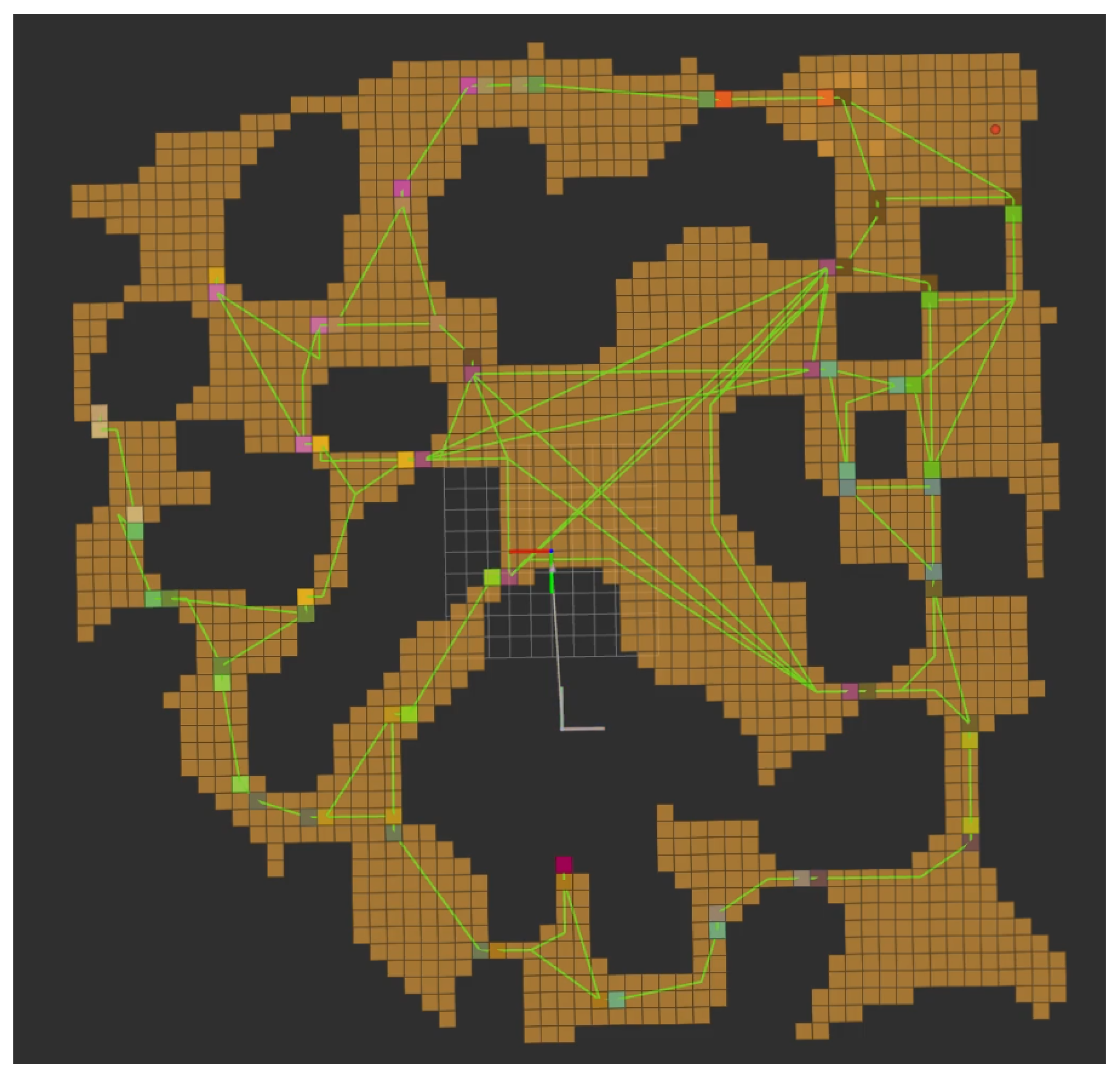
Evaluation of the framework was conducted with three sets of trials performed on the same randomly generated environment. The shape of the evaluation environment can be seen in Figure 18. A video can be found on the NanoMap Youtube Channel (https://youtu.be/FWLTIBuQVEw (accessed on 26 June 2023)) showing a selection of these trials. In the case of all trials, the time to complete a full search of the environment was recorded.

Table 7. Trial results.

Global Planner Trials
Agents	1	2	3	4	5
Average Time (sec)	288.8	165.2	116.4	90.8	73.8
Framework Trials  w/o  added obstacles
Agents	1	2	3	4	5
Average Time (sec)	351.2	192.4	132.2	N/A	N/A
Framework Trials  w/ added obstacles
Agents	1	2	3	4	5
Average Time (sec)	380.8	218.8	148.4	N/A	N/A

details the results for all three trials, with Figure 19, Figure 20, Figure 21 and Figure 22 providing visualizations of the results of the trials.

The first trial was used to test the performance of the global planner. This global planner trial used a fixed action completion time to assess the impact of increasing the number of agents when using only the decentralized global planner. Five tests runs were conducted for each agent configuration, and the results were averaged. The completion time data for the global planner trials can be seen in Table 5 and Figure 19.

Additionally for this trial, the number of rooms searched by each agent was tracked. These values were organized from largest to smallest for each test and averaged to obtain an understanding of how increasing the number of agents for the test environment affects individual agent efficiency. These results can be seen in Figure 20.

As can be seen from Table 7 and Figure 19, increasing the number of agents improves the time to complete a full search of the environment, demonstrating that even with minimal information sharing the agents are able to coordinate to improve target-finding performance. The improvement gained tapers off for the five agent trials, and this is a result reinforced by Figure 20. Figure 20 shows that for the test environment used in the trials, the use of three agents results in the number of searched rooms being well distributed across all agents. Figure 20 shows that an additional fourth agent still contributes somewhat to the search but illustrates that a fifth agent contributes very little. This behavior can be considered a result of the size and shape of the environment. The global graph map of the environment is not large enough to meaningfully benefit from more than four agents, with only a small contribution provided by a fifth agent.

The second and third trials were conducted to test the performance of the full framework, combining the output of the local controller and global planner to complete a full search of the simulated environment with and without added obstacles. These trials were completed for one, two, and three agent configurations.

In both the second and third set of trials, four and five agent configurations were not tested as a result of a software limitation that could not be resolved in the time available. GPU-based Stable Baselines 3 inference of the transit and search models could only be performed for 3 agents on a single machine. Attempting to perform policy inference for four agents at a single time on a single machine resulted in instability that crashed the Python ROS nodes used to control the agents.

Figure 21 and Figure 22 visualize the results of these trials, illustrating that increasing the number of agents translates to an improvement in the search time of the environment during the full operation of the framework. The second trial demonstrates how each instance of the framework can plan and control an agent to cooperatively search a large, partially observable, simulated environment. The third trial demonstrates that the framework is still capable of performing in an environment with increased uncertainty in the form of additional unknown obstacles. The average search times increased slightly as a consequence of these randomly introduced and unknown features. Improving the local controller model definitions and adding a more varied assortment of objects and obstacles to the training environment would further increase the performance of the control policies when operating in the presence of unknown obstacles.

10. Conclusions

This work extends the NanoMap library to provide GPU-accelerated planning and path-finding functionality for the occupancy grids produced by the library. Additional extensions were performed to enable the training of agents that require simulated sensing and mapping using Stable Baselines 3 and other approaches that use OpenAI gym style environments. Furthermore, a framework was developed that combines the NanoMap library, a DEC-POMDP model-based global planner, a deep reinforcement learning-based local controller, and ROS to enable multi-agent search and target finding for problems with target and environment uncertainty in large and complex environments. Simulated testing demonstrates the performance of the full framework for one, two, and three agent configurations and the performance of the global planner was validated for one, two, three, four, and five agent configurations.

Core aims for future work are as follows:

• The development and integration of a method for managing localization uncertainty within NanoMap and the framework.
• Streamlining the usability of the framework to provide researchers a flexible and high performance multi-agent planning and control framework for their own robotic solutions.
• Validation of the framework with real-world testing.

Additional aims to improve the utility of the framework include:

• Increasing the types of global planner and local controller models supported and available for use with the framework by default.
• Adding support for dynamic environments and hazards to NanoMap.
• Increasing the types of sensors and sensor data supported by NanoMap.

References

1. Tomic, T.; Schmid, K.; Lutz, P.; Domel, A.; Kassecker, M.; Mair, E.; Grixa, I.L.; Ruess, F.; Suppa, M.; Burschka, D. Toward a fully autonomous UAV: Research platform for indoor and outdoor urban search and rescue. IEEE Robot. Autom. Mag. 2012, 19, 46–56. [Google Scholar] [CrossRef] [Green Version]
2. Hodgson, A.; Kelly, N.; Peel, D. Unmanned aerial vehicles (UAVs) for surveying marine fauna: A dugong case study. PLoS ONE 2013, 8, e79556. [Google Scholar] [CrossRef] [Green Version]
3. Rojas, A.J.; Gonzalez, L.F.; Motta, N.; Villa, T.F. Design and flight testing of an integrated solar powered UAV and WSN for remote gas sensing. In Proceedings of the 2015 IEEE Aerospace Conference, Big Sky, MT, USA, 7–14 March 2015; pp. 1–10. [Google Scholar]
4. Kersnovski, T.; Gonzalez, F.; Morton, K. A UAV system for autonomous target detection and gas sensing. In Proceedings of the 2017 IEEE Aerospace Conference, Big Sky, MT, USA, 4–11 March 2017; pp. 1–12. [Google Scholar]
5. Borie, R.; Tovey, C.; Koenig, S. Algorithms and complexity results for graph-based pursuit evasion. Auton. Robot. 2011, 31, 317–332. [Google Scholar] [CrossRef]
6. Ward, S.; Hensler, J.; Alsalam, B.; Gonzalez, L.F. Autonomous UAVs wildlife detection using thermal imaging, predictive navigation and computer vision. In Proceedings of the 2016 IEEE Aerospace Conference, Big Sky, MT, USA, 5–12 March 2016; pp. 1–8. [Google Scholar]
7. Gohl, P.; Burri, M.; Omari, S.; Rehder, J.; Nikolic, J.; Achtelik, M.; Siegwart, R. Towards autonomous mine inspection. In Proceedings of the 2014 3rd International Conference on Applied Robotics for the Power Industry, Foz do Iguacu, Brazil, 14–16 October 2014; pp. 1–6. [Google Scholar]
8. Walker, V.; Vanegas, F.; Gonzalez, F. NanoMap: A GPU-Accelerated OpenVDB-Based Mapping and Simulation Package for Robotic Agents. Remote Sens. 2022, 14, 5463. [Google Scholar] [CrossRef]
9. Feroz, S.; Abu Dabous, S. Uav-based remote sensing applications for bridge condition assessment. Remote Sens. 2021, 13, 1809. [Google Scholar] [CrossRef]
10. Sondik, E.J. The optimal control of partially observable Markov processes over the infinite horizon: Discounted costs. Oper. Res. 1978, 26, 282–304. [Google Scholar] [CrossRef]
11. Kurniawati, H.; Yadav, V. An online POMDP solver for uncertainty planning in dynamic environment. In Robotics Research; Springer: Berlin/Heidelberg, Germany, 2016; pp. 611–629. [Google Scholar]
12. Silver, D.; Veness, J. Monte-Carlo planning in large POMDPs. Adv. Neural Inf. Process. Syst. 2010, 23. [Google Scholar]
13. He, R.; Brunskill, E.; Roy, N. PUMA: Planning Under Uncertainty with Macro-Actions. In Proceedings of the AAAI Conference on Artificial Intelligence, Atlanta, GA, USA, 11–15 July 2010. [Google Scholar]
14. Vanegas, F.; Gonzalez, F. Enabling UAV navigation with sensor and environmental uncertainty in cluttered and GPS-denied environments. Sensors 2016, 16, 666. [Google Scholar] [CrossRef] [PubMed] [Green Version]
15. Zhu, X.; Vanegas, F.; Gonzalez, F. An approach for multi-UAV system navigation and target finding in cluttered environments. In Proceedings of the 2020 International Conference on Unmanned Aircraft Systems (ICUAS), Athens, Greece, 1–4 September 2020; pp. 1113–1120. [Google Scholar]
16. Galvez-Serna, J.; Vanegas, F.; Brar, S.; Sandino, J.; Flannery, D.; Gonzalez, F. UAV4PE: An open-source framework to plan UAV autonomous missions for planetary exploration. Drones 2022, 6, 391. [Google Scholar] [CrossRef]
17. Ebert, F.; Finn, C.; Dasari, S.; Xie, A.; Lee, A.; Levine, S. Visual foresight: Model-based deep reinforcement learning for vision-based robotic control. arXiv 2018, arXiv:1812.00568. [Google Scholar]
18. Lillicrap, T.P.; Hunt, J.J.; Pritzel, A.; Heess, N.; Erez, T.; Tassa, Y.; Silver, D.; Wierstra, D. Continuous control with deep reinforcement learning. arXiv 2015, arXiv:1509.02971. [Google Scholar]
19. Badia, A.P.; Piot, B.; Kapturowski, S.; Sprechmann, P.; Vitvitskyi, A.; Guo, Z.D.; Blundell, C. Agent57: Outperforming the atari human benchmark. In Proceedings of the International Conference on Machine Learning, Online, 13–18 July 2020; pp. 507–517. [Google Scholar]
20. Maciel-Pearson, B.G.; Marchegiani, L.; Akcay, S.; Atapour-Abarghouei, A.; Garforth, J.; Breckon, T.P. Online deep reinforcement learning for autonomous UAV navigation and exploration of outdoor environments. arXiv 2019, arXiv:1912.05684. [Google Scholar]
21. Qie, H.; Shi, D.; Shen, T.; Xu, X.; Li, Y.; Wang, L. Joint optimization of multi-UAV target assignment and path planning based on multi-agent reinforcement learning. IEEE Access 2019, 7, 146264–146272. [Google Scholar] [CrossRef]
22. Xue, Z.; Gonsalves, T. Vision based drone obstacle avoidance by deep reinforcement learning. AI 2021, 2, 366–380. [Google Scholar] [CrossRef]
23. Anwar, A.; Raychowdhury, A. Autonomous navigation via deep reinforcement learning for resource constraint edge nodes using transfer learning. IEEE Access 2020, 8, 26549–26560. [Google Scholar] [CrossRef]
24. Sapio, F.; Ratini, R. Developing and Testing a New Reinforcement Learning Toolkit with Unreal Engine. In Proceedings of the International Conference on Human-Computer Interaction, Online, 26 June–1 July 2022; pp. 317–334. [Google Scholar]
25. Sanders, J.; Kandrot, E. CUDA by Example: An Introduction to General-Purpose GPU Programming; Addison-Wesley Professional: Boston, MA, USA, 2010. [Google Scholar]
26. Yang, S.; Liu, X.; Wang, Y.; He, X.; Tan, G. Fast All-Pairs Shortest Paths Algorithm in Large Sparse Graph. In Proceedings of the 37th International Conference on Supercomputing, Orlando, FL, USA, 21–23 June 2023; pp. 277–288. [Google Scholar]
27. Campos, C.; Elvira, R.; Rodríguez, J.J.G.; Montiel, J.M.; Tardós, J.D. Orb-slam3: An accurate open-source library for visual, visual–inertial, and multimap slam. IEEE Trans. Robot. 2021, 37, 1874–1890. [Google Scholar] [CrossRef]
28. Xu, X.; Zhang, L.; Yang, J.; Cao, C.; Wang, W.; Ran, Y.; Tan, Z.; Luo, M. A review of multi-sensor fusion slam systems based on 3D LIDAR. Remote Sens. 2022, 14, 2835. [Google Scholar] [CrossRef]
29. Wang, S.; Wang, Y.; Li, D.; Zhao, Q. Distributed Relative Localization Algorithms for Multi-Robot Networks: A Survey. Sensors 2023, 23, 2399. [Google Scholar] [CrossRef]
30. Kim, P.; Kim, J.; Song, M.; Lee, Y.; Jung, M.; Kim, H.G. A benchmark comparison of four off-the-shelf proprietary visual–inertial odometry systems. Sensors 2022, 22, 9873. [Google Scholar] [CrossRef]
31. Maruyama, Y.; Kato, S.; Azumi, T. Exploring the performance of ROS2. In Proceedings of the 13th International Conference on Embedded Software, Chengdu, China, 13–14 August 2016; pp. 1–10. [Google Scholar]
32. Museth, K.; Lait, J.; Johanson, J.; Budsberg, J.; Henderson, R.; Alden, M.; Cucka, P.; Hill, D.; Pearce, A. OpenVDB: An open-source data structure and toolkit for high-resolution volumes. In Proceedings of the Acm Siggraph 2013 Courses, Anaheim, CA, USA, 21–25 July 2013; p. 1. [Google Scholar]
33. Walker, O.; Vanegas, F.; Gonzalez, F. A framework for multi-agent UAV exploration and target-finding in GPS-denied and partially observable environments. Sensors 2020, 20, 4739. [Google Scholar] [CrossRef]
34. Klimenko, D.; Song, J.; Kurniawati, H. TAPIR: A Software Toolkit for Approximating and Adapting POMDP Solutions Online. In Proceedings of the Australasian Conference on Robotics and Automation, Melbourne, Australia, 2–4 December 2014; Volume 24. [Google Scholar]
35. Raffin, A.; Hill, A.; Ernestus, M.; Gleave, A.; Kanervisto, A.; Dormann, N. Stable baselines 3. J. Mach. Learn. Res. 2021, 22, 1–8. [Google Scholar]
36. Haarnoja, T.; Zhou, A.; Abbeel, P.; Levine, S. Soft actor-critic: Off-policy maximum entropy deep reinforcement learning with a stochastic actor. In Proceedings of the International Conference on Machine Learning, Stockholm, Sweden, 10–15 July 2018; pp. 1861–1870. [Google Scholar]
Figure 1. Multi-agent configuration.
Remotesensing 15 03802 g001
Figure 2. Planning and control framework.
Remotesensing 15 03802 g002
Figure 3. Reducing an occupancy grid to the SAFE nodes of a P-Grid. (a) Example environment occupancy grid. (b) SAFE nodes of example environment P-Grid.
Remotesensing 15 03802 g003
Figure 4. Environment reduced further, removing disconnected regions that are considered inaccessible. (a) P-Grid containing inaccessible regions. (b) Continuous P-Grid with inaccessible regions removed.
Remotesensing 15 03802 g004
Figure 5. A cluster generated while segmenting the environment.
Remotesensing 15 03802 g005
Figure 6. Shortest path through a concave polygon from start location (orange) to goal location (green) traverses a vertex (blue).
Remotesensing 15 03802 g006
Figure 7. Edges and vertices in 2D and 3D space (a) 2D vertex (green) to occupied cells (red). (b) 3D vertex (green) and edges (orange) to occupied cells (red).
Remotesensing 15 03802 g007
Figure 8. Further reducing the working cluster grids to their vertex nodes to reduce the solution complexity. (a) SAFE nodes of P-Grid. (b) Vertex nodes of P-Grid.
Remotesensing 15 03802 g008
Figure 9. 2D cluster path solve example. (a) Vertex nodes (blue), start node (green), and destination node (orange). (b) Closest vertices for start and destination retrieved, along with path between those vertices (blue). (c) Line of sight is checked for start and destination nodes against path nodes. (d) Final path retrieved, skipping unnecessary nodes.
Remotesensing 15 03802 g009
Figure 10. Calculating the global shortest path on a simplified 2D environment. (a) A 2D example environment with border nodes (purple), vertex nodes (blue), and a start node (orange). (b) Calculating the path to the target node (green) by comparing the length of the precomputed paths between border points (purple).
Remotesensing 15 03802 g010
Figure 11. Global planner.
Remotesensing 15 03802 g011
Figure 12. Global environment abstraction. (a) 2D view of example environment with calculated paths (green lines) between clusters (b) Abstracted graph representation of environment used by global planner.
Remotesensing 15 03802 g012
Figure 13. Global planner agents and their observations in the environment. Agent 1 (orange): In Node 1, has not completed a search in this node. Agent 2 (green): In Node 29, completed a search in this node and has not found the target. Agent 3 (purple): In Node 8, has completed a search in this node and has found the target.
Remotesensing 15 03802 g013
Figure 14. Local controller.
Remotesensing 15 03802 g014
Figure 15. Agent observations: (a) hazard observations (red), (b) unknown observations (orange), and (c) agent moving toward goal (purple sphere) while building map using simulated camera.
Remotesensing 15 03802 g015
Figure 16. Deep reinforcement learning simulation loop.
Remotesensing 15 03802 g016
Figure 17. Framework software architecture.
Remotesensing 15 03802 g017
Figure 18. 50 m × 50 m evaluation environment. Computed boundary points between clusters (coloured squares). Planner calculated paths between boundary points (green lines).
Remotesensing 15 03802 g018
Figure 19. Global planner trial search times.
Remotesensing 15 03802 g019
Figure 20. Agent search efficiency. Bar colours map to the scores received from the most effective agent to the least effective agent for any given agent configuration and test using the following order: orange (most effective), green, blue, purple, and red (least effective).
Remotesensing 15 03802 g020
Figure 21. Full framework search times (without unknown obstacles).
Remotesensing 15 03802 g021
Figure 22. Full framework search times (with randomly added unknown obstacles).
Remotesensing 15 03802 g022