Article

High-Resolution Image Products Acquired from Mid-Sized Uncrewed Aerial Systems for Land–Atmosphere Studies

Pacific Northwest National Laboratory (PNNL), Richland, WA 99352, USA
*
Author to whom correspondence should be addressed.
These authors also contributed equally to this work.
Remote Sens. 2023, 15(16), 3940; https://doi.org/10.3390/rs15163940
Submission received: 28 June 2023 / Revised: 3 August 2023 / Accepted: 3 August 2023 / Published: 9 August 2023

Abstract

:
We assess the viability of deploying commercially available multispectral and thermal imagers designed for integration on small uncrewed aerial systems (sUASs, <25 kg) on a mid-size Group-3-classification UAS (weight: 25–600 kg, maximum altitude: 5486 m MSL, maximum speed: 128 m/s) for the purpose of collecting a higher spatial resolution dataset that can be used for evaluating the surface energy budget and effects of surface heterogeneity on atmospheric processes than those datasets traditionally collected by instrumentation deployed on satellites and eddy covariance towers. A MicaSense Altum multispectral imager was deployed on two very similar mid-sized UASs operated by the Atmospheric Radiation Measurement (ARM) Aviation Facility. This paper evaluates the effects of flight on imaging systems mounted on UASs flying at higher altitudes and faster speeds for extended durations. We assess optimal calibration methods, acquisition rates, and flight plans for maximizing land surface area measurements. We developed, in-house, an automated workflow to correct the raw image frames and produce final data products, which we assess against known spectral ground targets and independent sources. We intend this manuscript to be used as a reference for collecting similar datasets in the future and for the datasets described within this manuscript to be used as launching points for future research.

1. Introduction

The ability to forecast the earth–atmosphere system relies on the comprehension of the mechanisms influencing the surface energy balance between the land surface and atmosphere [1,2,3,4]. The observational datasets on which this foundational knowledge has been built have traditionally relied on two sources: satellite imagery [5,6,7,8] and in situ surface measurements (towers) [1,4,9,10].
Land surface imagery traditionally used in atmospheric research comes from earth observation satellites including the Moderate Resolution Imaging Spectroradiometer (MODIS) [11], Landsat [12], Sentinel-2 [13], and other government-operated systems. These systems operate in sun-synchronous polar orbits and continually collect data at varying resolutions and revisit times [14]. While the observational data collected by satellites are useful for a plethora of studies, these data may not be suitable for applications which require either temporal control, since they are limited to revisit times determined by satellite orbits and cloud cover, or a spatial resolution finer than 10 m.
The data that inform the surface energy balance provided by flux or eddy covariance towers are from a staple of studies of land–atmosphere interactions and boundary layer meteorology [15]. The basic configuration of these systems consists of a net radiometer and sonic anemometer. While tower instrumentation is not weight- or power-constrained, its fixed location at a single altitude limits measurements to the surrounding environment. These individual sites can be used together as a network, such as FLUXNET, or to create a ‘site-averaged dataset’ [2,3,10,16]. Airborne measurements, though limited by payload weight and power usage, can overcome these platform limitations, sampling across a wider area than towers can provide and at a cadence and schedule that satellites cannot match.
One recent advancement to fill this gap has been the use of sUASs (<25 kg) with multispectral imager payloads. These multispectral imagers have been tested thoroughly on sUASs and have been featured in numerous publications [17,18,19]. These systems offer an advantage over satellite imagery in their ability to provide thermal and visible imagery at a higher resolution (~4 cm/pixel) and have been deployed successfully in the areas of precision agriculture, forestry, and civil engineering [20,21,22,23]. They are quick to deploy and redeploy, generally fly up to an altitude of 120 m Above Ground Level (AGL), and have a battery life of 20–40 min, capturing surface imagery at a ground speed of ~15 m/s. These imagers usually capture RGB, red-edge, and near-infrared (NIR) data, but some are equipped to synchronically collect thermal imagery (long-wave infrared; LWIR) while others collect hyperspectral wavelengths. The thermal imagery provides greater surface detail than infrared thermometers deployed on the same platform because the thermal imagers measure skin temperature for every pixel within the field of view. The raw image frames are aligned and stitched together to create high-resolution-image products, which are rectified via ground control points to create orthomosaics. Using the technique of structure from motion, the processing software can also create digital elevation models of the bare ground and canopy surface [24]. The calibrated multispectral data can be combined to derive atmospherically relevant surface properties such as albedo, surface reflectance, skin temperature, and various vegetative indices. It has been demonstrated that calibrated orthomosaics with one or two source energy budget models can be used to map surface radiation, improving upon the single point source that a flux station provides [25]. Using an sUAS as a platform to study the surface energy budget and assess surface heterogeneity is constrained by its limited battery lifetime and area coverage [26].
A better platform for assessing land surface–atmospheric coupling is a mid-size (Group 3) UAS (>25 kg and <600 kg) that can deploy continuously for multiple hours one to two times a day and can image an area suitable for cloud-resolving model spatial boundaries (~km2) at a spatial resolution on the order of ~1 m, one to two orders of magnitude greater than the current datasets used for atmospheric/land interaction studies. These platforms capture land surface imagery with repeatable accuracy via programmable flight plans and adaptable autopilots that adjust to the current wind vectors [27].
However, there are challenges with deploying these imagers designed for sUASs on mid-size UASs. Land surface images taken from higher altitudes may introduce artifacts from aerosol and water vapor scattering/absorption in the air column. When flying for longer durations, there will be fluctuations in irradiance due to changing solar angles and variability in the aerosol and water vapor concentration across the collection area [26]. In addition, the aircraft will experience stronger winds aloft, causing large differences in ground speed as the aircraft experiences headwinds and tailwinds, affecting the fidelity of the final orthorectified product. Additionally, a fixed-wing mid-size UAS is not as nimble as an sUAS. Thus, the aircraft will spend more time maneuvering to line up with the next flight line.
In this paper we address these challenges directly, evaluating calibration methodologies that include the use of reflectance tarps along our flight path for empirical line fit reflectance corrections. We experiment with different flight planning strategies and image capture techniques that ensure proper image overlap and capture with minimal time in the air. The utilization of the data from the downwelling light sensor version 2 (DLS2) to correct for changing solar illumination conditions is discussed. An intercomparison of the Altum thermal imager covering the same wavelength and a similar field of view (FOV) with a thermal infrared thermometer (IRT) onboard the UAS is also shown. Finally, we present orthomosaics generated in flight and propose future work and applications of this dataset.

2. Materials and Methods

The data presented in this paper were captured during flights with a mid-size, Group 3 UAS in November 2021 over the Department of Energy Atmospheric Radiation Measurement (ARM) Southern Great Plains (SGP) site and in February 2023 within the Pendleton, Oregon, UAS Range (PUR). The imager used in all flights is the Altum developed by MicaSense. The post-processing routine was developed at the Pacific Northwest National Laboratory (PNNL) using elements from MicaSense’s Python tools and the United States Geological Survey’s guide to structure-from-motion photogrammetry using the imagery processing software Agisoft MetaShape [28]. The final imagery products are orthomosaics with TIF extensions with reflectance values for red, green, blue, red-edge, near IR, and long-wave IR (thermal) bands and a digital elevation model (DEM).

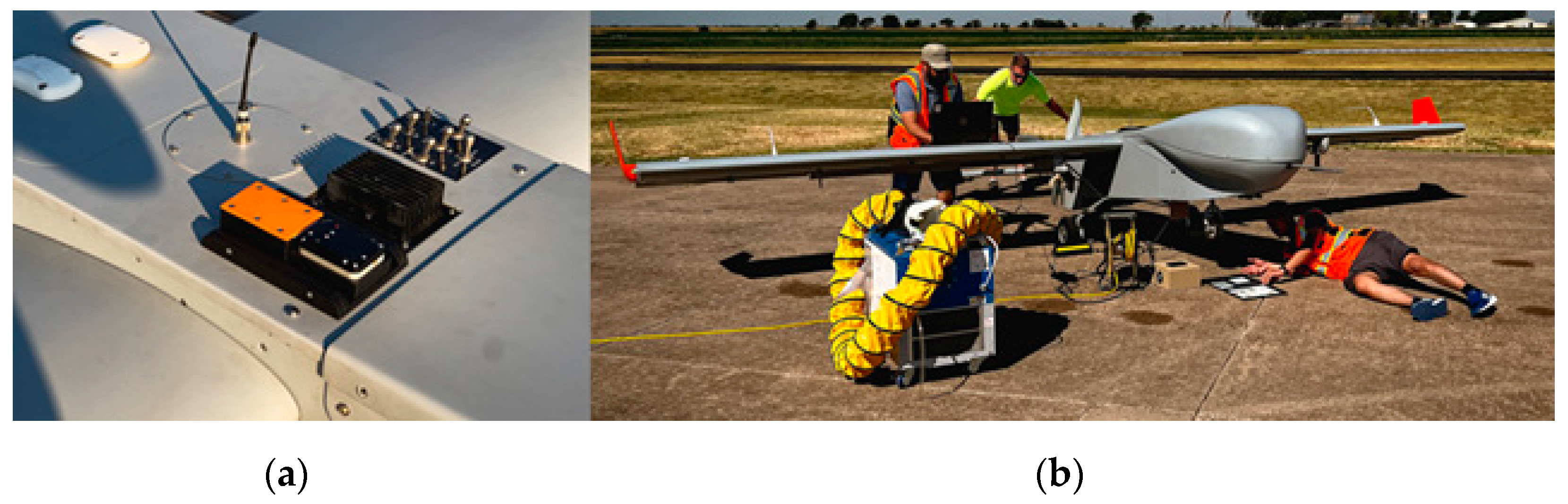
2.1. Mid-Size UAS Description

The ARM Aerial Facility (AAF) [29] has been operating the Navmar Science Corporation (NASC, Warminster, PA, USA) ArcticShark Uncrewed Aerial System (UAS) since 2017 [30]. The ArcticShark is a custom-built variant (TS-B3-XP-AS) of the standard TigerShark Block 3 (TS-B3-XP) UAS, which is optimized for routine atmospheric sampling with the addition of a variable pitch propeller, lower noise profile, lower vibration levels, and 3 kW of payload power [31]. The conditions of flight are more akin to a general aviation aircraft than a fixed-wing or multirotor sUAS. While the ArcticShark was undergoing upgrades and modifications in 2021, the AAF staff collaborated with the Mississippi State University (MSU) Raspet Flight Research Laboratory (RFRL) to fly the ArcticShark scientific payload on an RFRL TS-B3-XP TigerShark. A description of all the datasets obtained from the AAF payload can be found here [32]. A comparison between the TigerShark XP and ArcticShark is shown in Table 1.
The aircraft is operated using Cloud Cap’s Piccolo autopilot, which allows for repeatable, pre-programmed flight plan execution. The autopilot produces a log of aircraft performance variables including pitch, roll, and yaw, which can be compared to the imager’s metadata.

2.2. Altum Imager and Calibration

The MicaSense Altum imager is a commercial off-the-shelf synchronized multispectral and thermal camera combined with a GPS unit and downwelling light sensor [33]. The Altum sensor captures multispectral images of the land surface across five optical bands (48° horizontal FOV (HFOV) × 36.8° vertical FOV (VFOV)) and one long-wave infrared thermal band (57° HFOV × 44.3° VFOV). The spectral bands details are shown in Table 2. In the optical bands, the sensor measures reflected radiance and converts it to digital numbers (DN) using calibration coefficients. The emitted thermal data are recorded in the same manner.
The imager was mounted to the ventral side of each aircraft in the main payload bay. The camera was installed in the payload bay in a custom 3D printed case in the “landscape” position such that the HFOV was maximized for image overlap. The assembly was mounted directly to the aircraft rather than on a gimble to avoid obstructing the path of air feeding the engines. This configuration limits usable images to those collected during ‘straight and level’ flight, which we defined as ±3° in pitch and roll.
The DLS2 light sensor was mounted on the dorsal side of the aircraft on a custom plate parallel to the aircraft’s angle of attack from which it could be easily unclipped for pre-flight magnetometer calibrations (see Figure 1a). For our configuration, we used the DLS2’s integrated GPS for positional accuracy. Images were captured every 2 s, which provided sufficient time for the completion of the automatic thermal non-uniformity correction (NUC) for changing internal temperature of the sensor. The imager was powered from the aircraft’s onboard data acquisition system. Horizontal overlap was accounted for when creating the UAS’s preprogrammed flight plans for image capture.
The DLS2 provided synced measurements of direct and diffuse irradiance and sun-to-sensor angle. This information was recorded in the metadata of the TIFF images. These measurements were used to correct for changing lighting conditions along the flight path (such as changing cloud cover).
The standard calibration practice for collecting calibration data for an Altum multispectral camera is to take pre- and post-flight images of a calibration panel (15 × 15 cm) of known reflectance; see Figure 1. However, this method was infeasible for a mid-size UAS. To image the panel, the entire platform had to be tilted, resulting in different incoming solar incidence angles for the DLS2 unit and the panel. Additionally, post-flight panel captures with both the DLS2 and panel in sunlight were not possible due to the high solar elevation angle and the bulbous nose of the ArcticShark casting shadows on the panel. This calibration method was determined to be infeasible for mid-sized UASs. Instead, Tetracam™ calibration tarps with 11% and 48% absolute reflectance in the range of 400 nm to 850 nm were routinely imaged by the camera while in flight (See Figure 2). This method provided a far more accurate calibration and could be used to assess impacts from aerosol and water vapor (scattering) on measured surface reflectance.
For validation of the MicaSense™ thermal imager, a ventral Apogee SI-411-SS infrared thermometer (IRT) with a 44° FOV was flown. The Apogee IRT samples 60% of the Altum thermal sensor surface area. In our sampling area at the DOE ARM Southern Great Plains atmospheric observatory, there were a 25 m and a 10 m tower with a down-looking IRT (Heitronics 700). These Apogee and Heitronics IRTs have been compared over asphalt with good agreement [34].
One feature of operation which differed greatly between operating this camera on an sUAS and on a mid-size UAS was the treatment of target altitude. sUASs are generally flown under 14 CFR part 107 guidelines to a maximum altitude of 120 m (400 ft). Therefore, altitude control of these platforms by their autopilot is treated as a range between target altitude and a lower limit (target altitude − X). For larger aircraft, the programmed altitude is thought of as having a tolerance range treated as target altitude ± X. The Altum imager’s capture range is designed to be programmed using the sUAS method. Therefore, to set the Altum’s image capture to match the mid-size UAS’s flight altitude in the software, we use Formula (1).
Target Altitude|True = Target Altitude|Programmed − X [m],
X = desired range ± altitude
2 × X = programmed range 

2.3. Flight Pattern Development

The objective of the pre-programmed flight pattern is to acquire images with sufficient overlap between frames to derive a topographic surface while minimizing the time aloft. Completing the acquisition as quickly as possible minimizes the change in solar and atmospheric conditions. An overlap of 75% was adopted based on the software vendor’s recommendation for orthomosaic production. If 75% overlap is not achieved, the processing routine renders it as a gap or blank space in the final orthomosaic. For these deployments, a flight pattern commonly referred to as a “lawn mower” was used to capture imagery across a broad area. Initial flight patterns had the ArcticShark fly the sampling legs sequentially and covered an area of 10 km2. At 610 m AGL, the flight legs were 95 m apart to maintain 75% overlap between adjacent images (Figure 3). Because the turning radius of the aircraft significantly exceeds 0.5 × 95 m, this flight pattern resulted in rapid, banked (teardrop) turns at the end of the legs. This additional maneuvering greatly increased the flight time to 90 min for completion.
A more efficient method is to fly an alternating leg pattern where the turns can be planned to match the mid-size UAS’s turning radius. The alternating leg flight plan was first tested in the ArcticShark’s Piccolo flight simulator, which was developed by Cloud Cap. For a 9.2 km2 coverage, the flight was predicted to take an estimated 60 min at 610 m, with 95 m horizontal spacing between legs, and 30 min at 1220 m, with spacing between legs increased to 61 m. The benefits of flying higher and reducing sampling time are that it reduces changes in lighting conditions during sampling and saves on flight costs. During flight operations in February 2023, the ArcticShark flew the alternating leg pattern (Figure 3) at 915 m AGL, covering 7 km2 in 45 min, verifying the flight simulator estimates. This amount of time is nominally the same as it takes to capture a 1 km2 area with an sUAS platform.
Horizontal overlap is solely dependent on HFOV, the aircraft altitude, and the width of the flight legs, all of which are known before flight. The forward overlap is dependent on VFOV, the aircraft altitude, and ground speed. Only true airspeed (TAS) can be programmed by the Piccolo autopilot, not ground speed. Ground speed can be variable in flight due to winds aloft, and thus, there is no single capture rate that can be used to precisely maintain 75% overlap throughout the flight. The aircraft’s true airspeed is typically around 33 m/s, and 26 m/s is the fastest wind speed aloft at which the aircraft can operate. Thus, without winds, the ground speed is 33 m/s, and the maximum ground speed the UAS can theoretically experience in flight is 59 m/s. To ensure that the capture rate at a planned flight altitude is equal to or greater than 2 s, the capture rate is calculated using Equation (2). Sample capture rates are listed in Table 3. The practical reason for calculating capture rate rather than defaulting to an acquisition rate of 2 seconds is to reduce data storage and post-processing time.
T c a p t u r e = 1 O G s A 2 tan 1 2 V F O V ,
Tcapture = capture rate (s)                         
Gs = ground speed (m/s)                         
O = fractional overlap (e.g., 0.75 = 75%)
A = altitude (m)                                       
VFOV = vertical field of view (°)           
The variability in the ground speed, however, can be reduced by flying perpendicular to the wind direction, as shown in Figure 3. During flight operations in February 2023, this methodology was successfully demonstrated with the aircraft flying at a TAS of 33.3 ± 1 m/s in 15 m/s winds from 223°. The headings of the legs (155° and 335°) were determined by utilizing the North America Model (NAM) prediction of winds from 245°. Although this prediction was slightly incorrect, the ground speed on the 155° legs was 26 ± 1.4 m/s, and on the 335° legs, it was 37.5 ± 1.6 m/s. This 11.6 m/s difference in ground speed was roughly three times better than the 30 m/s expected difference had the aircraft flown parallel to the winds. The aircraft’s average crab angle (difference in the yaw direction from the heading) of 24.8 ± 40 had no impact on the ability to generate a merged mosaic. A second way to mitigate the impact of wind resistance is to fly at higher altitudes, as the camera does not require as fast an acquisition rate to maintain adequate frame overlap.

2.4. Post-Processing

Post-processing is the routine used to create analysis quality orthomosaics from individual raw frames. The first step is to apply radiometric corrections to each individual frame and convert the data from radiance images to reflectance. The next step involves stitching the images together to create an orthorectified mosaic, or orthomosaic, of the land surface with a corresponding DEM. Finally, we perform an empirical line fit to validate the reflectance measured at each altitude of image capture.
Each image is corrected for the sensor calibration, lens distortions, vignette effects, sun angle, and atmospheric effects (scattering and absorption). Traditionally with an sUAS, the standard operating procedure to convert UAS multispectral data to reflectance is to take pre- and post-flight measurements over an anisotropic target with known spectral properties (e.g. the panels mentioned in Section 2.3). These measurements are then used to calculate a coefficient to convert the DN directly to reflectance for each band in every image. Successful use of this procedure assumes that incoming solar radiation remains constant during the flight (constant lighting conditions). Such an assumption is frequently justified when flying short missions over small areas (10–20 min) but becomes problematic for longer missions and those taking place under partial cloud cover. Neither assumption is met for our application, requiring the development of an alternate processing workflow for the MicaSense data.
Since the longer flight times of mid-sized UASs result in changing solar conditions, we incorporate the DLS data into our correction approach. While in flight, the DLS2 measures incoming solar irradiance and sun angle at the precise time of image capture for each of the five bands of the camera and records this information in the metadata of the images. To calculate the apparent reflectance for each image frame, we ratio the DLS2 band spectral irradiance value to the radiance measured at the sensor (Equation (3)).
Rλ = π × Lλ/Iλ,
Rλ = band reflectance               
  Lλ = band radiance from image
   Iλ = band irradiance from DLS2
These data were further corrected by referencing the reflectance tarp values to determine empirical line fit coefficients for each band specific to a particular flight altitude. The corrected images were then input to the photogrammetry software Agisoft Metashape v1.4 to align and stitch the images into a larger composite image. The resulting image mosaics have a resolution of 20–60 cm/pixel depending on the altitude at which they were taken.
Our processing script follows the published USGS workflow to apply the structure from motion image algorithm in Agisoft to construct a dense cloud and 3D model of the surface [28]. The 3D model is used to produce a raster DEM of the area of image capture.
The final mosaics can be used to calculate leaf area index, albedo, and various other vegetative indices, such as Normalized Difference Vegetation Index (NDVI), Green Normalized Difference Vegetation Index (GNDVI), Normalized Difference Water Index (NDWI), surface temperature, and Enhanced Vegetation Index (EVI). From the thermal band, a mosaic of skin surface temperature is produced, and these measurements can be used to calculate evapotranspiration of vegetation crop stress indices.
We based our quantitative geometric and radiometric corrective schema on that described in Iqbal et al. 2018 [35]. The three-part semi-automated Python workflow we created is tailored for routine deployments, with user input required to specify the number of flying levels and the location of calibration tarps. The first script runs the uncorrected imagery through the MicaSense Python radiometric correction code so that the images are corrected for dark level, row gradient, and radiometric calibration to radiance. The second script uses Agisoft Metashape API code and automates the processes that would normally be done in the Agisoft Metashape GUI. Following the guidance of the USGS structure from motion workflow, we added parameters for camera alignment and gradual selection [24]. In the final part of the workflow, the empirical line fit is applied to the orthomosaics using published reflectance values for the tarps imaged at each flying level.
While not entirely open-source due to the licensing of Agisoft, our code, sample imagery data, and a step-by-step user guide are available for download via the ARM repository, and can be adapted for other imagery software APIs (such as Pix4d™), (https://github.com/ARM-DOE/camspec-air-processing, accessed on 23 July 2023). Both the unprocessed imagery collected and the final processed orthomosaics are available for download from the ARM archive (https://adc.arm.gov/discovery/#/results/s::camspec-air, accessed on 23 July 2023).

3. Results

The quality of orthomosaics produced with the Altum multispectral camera on a Group 3 UAS are discussed below. We found that this imager can collect surface data with a spatial resolution O(1 m), surpassing published datasets used for atmospheric science research, which use O(10–100 m) [3,6]. The orthomosaics of the caliber we produced can be used to probe the effects of surface heterogeneity at cloud resolving scales and at higher spatial resolutions than previous studies [2].

3.1. Calibration

Instead of the calibration panel, tarps of known reflectance, 11% and 48%, were overflown at multiple altitudes between 520–1360 m AGL (900–1740 m MSL) for calibration. Observing the tarps at different altitudes enabled the assessment of the effect of atmospheric scattering on data quality in addition to impacts from aerosol and water vapor. Figure 4 shows the published tarp reflectance values and mean 3 × 3 neighborhood pixel reflectance values centered on the tarps calculated for each altitude. For all altitude levels, individual tarps covered an area consisting of dozens of pixels and we selected a centered 3 × 3 subset of pixels to ensure that the neighborhood did not include edge values. We would expect more pronounced atmospheric scattering in the shortest wavelengths, thereby increasing the reflectance values in the corresponding bands. This effect would be especially noticeable over the dark target. We saw no such increase in reflectance values over either tarp, and in some cases, a decrease was observed. The apparent differences between the published tarp values and pixel values for the tarp images are likely due to noise in the DLS2 measurements used to ratio the image radiance values to reflectance. These data provided a valuable check, and the DLS2 sensor was returned to the vendor to further investigate the source of the offset.

3.2. Data Quality and Validation

3.2.1. Thermal Imagery Comparison to Infrared Thermometers

The IRT flown on the TigerShark (and ArcticShark) was an Apogee SI-411-SS that senses surface skin temperature using a thermopile [36]. Like the Altum thermal band, it also measures in the 8–14 μm wavelength range and has a similar FOV, allowing for excellent intercomparison between the sensors, as conducted in previous studies [37]. Serving as a further comparison, a 30 m tower at the SGP site is equipped with a Heitronics 700 IRT [38]. All three sensors were analyzed for flights covering the tower area. The aircraft Apogee and stationary Heitronics IRT sensors were compared only when their FOVs overlapped, demonstrating agreement within 0.25 °C during the day (Figure 5). The comparison of the UAS Apogee IRT to the Altum thermal band showed that the Altum sensor was, on average, 5 °C colder, which is consistent with the literature [34]. We believe that this is due to the thickness of the window on the thermal imager lens. Notably, Mei et al. found that the Apogee IRT surface temperature readings varied with altitude, likely resulting from changing internal temperature [32].
Referencing Figure 6, the aircraft flew a lawnmower pattern at 520 m AGL with the imager collecting images, climbed up to 1360 m AGL via a square based ladder pattern, and then performed a second lawn mower pattern at 1360 m AGL with the IRT and Altum in continuous operation. The reported surface temperature from the IRT decreased with altitude, affected by the colder temperatures aloft [32]. The Altum imager performs a thermal NUC correction for every 3° Celsius change in internal temperature. For the scatter plots, the thermal data within the FOV was averaged into a single point to compare the Altum thermal imagery with the IRT’s time series data. The Altum has a distinct cold bias when comparing skin surface temperature at both 520 and 1360 m AGL (Figure 6a,c). A weak trend in the bias is harder to detect (Figure 6a,b,d). A quantitative comparison is difficult as the IRT has a known dependence on internal temperature.

3.2.2. Multispectral Imagery: Comparison to Space-Born Multispectral and Hyperspectral Imagery

We compared the UAS imagery to satellite data for validation purposes over common ground features that were likely to be relatively stable—gravel pad, bare soil, and clear water (Figure 7). Two sources of multispectral satellite imagery were used for the comparison: DESIS and Sentinel-2. The DESIS hyperspectral sensor orbits on the US space station and collects data over the US at varying intervals. We downloaded a DESIS image for our area of interest, collected approximately four weeks before our mission (12 October 2021). The DESIS sensor has 235 bands of data, with five of those bands sharing a common center wavelength with Altum sensor bands. The Sentinel-2 platform, operated by the European Space Agency (ESA), consists of two satellites in complementary orbits. Each satellite carries a wide swath high-resolution multispectral imager with 13 spectral bands and collects data at a 10–60 m resolution every five days. We used Sentinel-2 data from an overpass on 11 October 2021.
Across the multispectral bands compared, the measurements taken from the Altum multispectral imager onboard the mid-sized UAS were within ±5% reflectance regardless of the surface sampled, with most samples within ±2% reflectance. The UAS measurements of the gravel pad had the best agreement to the satellite imagery, with four of five data points falling between the values of the satellite. This may have been because it was the least seasonally variable of the sampled surfaces between the sample dates, especially in the autumn, when the data were collected, which is a time period in Oklahoma in which the land surface can be markedly changed by precipitation and crop harvesting.

3.2.3. Other Validating Attributes

We can qualitatively assess the geometric and radiometric properties of imagery by inspecting the mosaics for distortion or holes in the final image. Using pre-programmed flight plans and the aircraft’s autopilot, we were generally able to achieve the necessary 75% image overlap required for aligning and mosaicking the images. The aircraft was successful in maintaining its flight path. In some cases where the aircraft flew nearly parallel with the winds, ground speed was elevated such that this overlap could not be achieved. Otherwise, using a capture rate of 2 seconds of overlap was sufficient to avoid distortion and gaps in the orthomosaics. We opted to disable hole filling to ensure that image distortion was minimized in the final mosaic.
Regarding the spatial accuracy of the orthomosaics, the Agisoft software performed an automated image-to-image alignment using the geometric information provided by the GPS inside the DLS2. No artifacts of misalignment are evident in the mosaics created from the individual image frames. The ground accuracy of the rectified orthomosaics was shifted from known features up to an offset of 18 m. To reduce this offset, ground control points can either be placed pre-flight or selected from distinct features in the image. Both methods would require human input to the workflow and were not employed here. Tight spatial accuracy was not a priority for this dataset; instead, the focus was on covering a large representative area of the sampled surface and processing with minimal human inputs. Image-to-image methods were tested to align the UAS image with a USGS orthophoto base, but the results were variable. The further refinement of these approaches is needed for incorporation into future versions of the automated workflow.

3.3. Final Products

Our final products include the multispectral data cube, thermal image, and a digital elevation model (DEM) stored as TIFF image mosaics. The multispectral reflectance imagery generated from each band can be leveraged to produce vegetative indices that shed light on different aspects of surface properties (e.g., Figure 8). The thermal imagery provides a distributed measure of skin temperature of the features in each pixel (soil, vegetation, water, etc.) The DEM provides high-resolution elevation information on both vegetation structure as well as topographic patterns across the image study area.
The final processed orthomosaics are available for download from the ARM archive (https://adc.arm.gov/discovery/#/results/s::camspec-air, accessed on 23 July 2023) [39].

4. Discussion and Conclusions

This manuscript may be used as a future reference for flying multispectral and thermal imagers on mid-sized UASs for atmospheric research. To account for variable ground speeds caused by the variable and stronger winds aloft, we recommend calculating the acquisition rate (Equation (2)) for each flight to ensure the 75% overlap required by certain post-processing routines. As we approach the threshold of the Altum’s fastest capture rate (1 Hz), the overlap requirements are limited by a ground speed of 59 m/s.
For the best calibration practices, we recommend using ground reference tarps placed in the target area to account for changing illumination conditions during extended flights. We developed an automated post processing workflow to address changing lighting conditions and the high volume of imagery collected. We assessed resulting orthomosaics against independent sources and found good agreement. While the 30–60 cm/pixel resolution of these orthomosaics is coarse compared to datasets captured on sUASs at lower altitudes (~4–10 cm/pixel) for precision agriculture science, civil engineering, etc., it is orders of magnitude finer than the data available in the atmospheric science community. Moreover, the lower spatial resolution is compensated by an increase in surface area captured. These types of datasets open new possibilities for informing and parameterizing surface energy budgets and the effects of surface heterogeneity on atmospheric processes. For example, the greater temporal flexibility of the UAS platform in this study could be used to sample evapotranspiration rates and leaf area index pre- and post-precipitation events. The future application of this processing routine can be used with the deployment of hyperspectral imagers for soil moisture detection or multispectral imagers with polarized lenses to enable target detection and classification. An ARM proposal call is scheduled to be announced in fall/winter 2024 to leverage this type of payload for scientific analysis.
As the computational complexity of models for land–atmosphere coupling increases, there is a community need for higher spatial resolution datasets to use for evaluation efforts and as initial and boundary condition data. For example, the state-of-the-art land surface model Noah-MP [40,41] has been used in convection-permitting resolutions at O(km) resolutions (He et al., 2019) [40] coupled with large eddy simulations (LES) at O(10–100 m) resolutions [41,42]. Such recent model developments will soon offer the possibility of representing land–atmosphere interactions at even finer scales, down to meters. This leaves many questions to be answered regarding the applicability of LSM model assumptions at such fine scales, requiring a large amount of evaluation data [2]. Not only are scales of modelling being refined, but new scientific questions are being posed, such as those regarding the impacts of urbanization and other human activities on the interactions between the land and atmosphere. Taken together, these considerations indicate a pressing demand for innovative data sources that can support the configuration and evaluation of current and future generations of models. Integrating UAS imagery into atmospheric modelling can play a part in meeting those demands. Reassessing what is currently known through model-based studies of land–atmosphere coupling at an unprecedentedly fine resolution can only be accomplished with commensurately higher resolution information about the surface driving conditions. This dataset will help drive advancement in the model complexity hierarchy from the idealized lower boundaries commonly used in LES today towards the highly complex and fully coupled models that the research community is progressing towards.

Author Contributions

L.G.—conceptualization and writing; I.G.-H.—software, formal analysis, writing review and editing; K.N.—software; H.M.—investigation; F.M.—writing review; J.T. (Jason Tomlinson)—supervision, writing review and editing; B.S.—funding acquisition, supervision, writing review and editing; J.T. (Jerry Tagestad)—data curation, writing review and editing. All authors have read and agreed to the published version of the manuscript.

Funding

This work has been supported by the Office of Biological and Environmental Research (OBER) at the US Department of Energy (DOE) via the Atmospheric Radiation Measurement (ARM) program. Battelle operates the Pacific Northwest National Laboratory (PNNL) for the DOE under contract DE-A06-76RLO 1830. The associated PNNL project number is 15990.

Data Availability Statement

The data are available at the ARM data repository under the name “camspec_air” and are free to download at adc.arm.gov [38,39]. A description of the IRT data [36] used in this analysis can be found in Mei et al. 2022 [32]. The ARM data center (ADC) includes sufficient metadata in each netCDF and TIF file to facilitate the user’s understanding and interpretation. This work is licensed under the Creative Commons Attribution 4.0 International License, a copy of which can be found at ARM.gov. The ARM Data repository follows FAIR data principles and has been accredited by the International Science Council CoreTrustSeal. The spectral imagery data submitted to the arvice follow the ARM data file standards [43]. The data are provided in tif and jpg format and use the naming convention: {site}{instrument}.{YYYYMMDD}.{HHMMSS}.{altitude(msl)}.{file ext}. For the orthomosaic tif images, there are six bands represented per pixel that represent surface reflectivity (skin temperature for the sixth band). For the DEM, each pixel represents an elevation. These images can be converted into gridded products that can be used for analysis. Raster calculations of these bands can produce albedo, leaf area index, skin temperature, and various vegetative indices (e.g., NDVI). The raw images are available on the archive as well but are not publicly displayed. To obtain a copy of the raw images, send an email directly to the ARM Data management center (adc@arm.gov) and the instrument mentor, Jerry Tagestad. An instrument webpage with a link to a handbook and a direct link to the data is provided here: https://arm.gov/capabilities/instruments/camspec-air (accessed on 23 July 2023). The code which was developed to process these images is available at the ARM Git repository: https://github.com/ARM-DOE/camspec-air-processing (accessed on 23 July 2023). While the code is open-source, Agisoft Metashape is a licensed software that is needed for parts of the software to run. Other Python libraries, which are free online, are needed to make the script work.

Acknowledgments

We acknowledge Colleen Kaul, PNNL and Koichi Sakaguchi, PNNL for their insightful knowledge about the current state of the atmosphere–land-surface interaction modelling community. We acknowledge the team of people who made these UAS operations possible. Air Vehicle Pilots: Stephen Hamilton, NASC, Brad Petty, NASC, Charley Zera, NASC, and Austin Wingo, MSU. Mission Commanders: Pete Carroll, PNNL, and Nolan Parker, MSU. UAS Technicians: Pete Carroll, PNNL, Mike Crocker, PNNL, Jonathan Stratman, PNNL, Andre Watson, PNNL, John Stephenson, PNNL, Conor White, MSU, and Miles Ennis, MSU. Payload Operators: Victor Aguilera-Vazquez, PNNL. Scientists: Mikhail Pekour, PNNL. Director of Flight Operations: Tim McLain, PNNL. Director of Maintenance: Andre Watson, PNNL. Visual Observers: Mike Hubbell, PNNL, Lupita Renteira, PNNL, Josh Torgenson, PNNL, Orlando Garayburu-Caruso, PNNL, Susanne Glienke, PNNL, Eric Fischer, PNNL, Clay Shires, MSU, Randy Welch, MSU, Cavin Skidmore, MSU, Peter McKinley, MSU, Taylor Eskridge, MSU, and Chase Jackson, MSU.

Conflicts of Interest

The authors declare no conflict of interest.

References

  1. Blyth, E.; Gash, J.; Lloyd, A.; Pryor, M.; Weedon, G.P.; Shuttleworth, J. Evaluating the JULES land surface model energy fluxes using FLUXNET data. J. Hydrometeorol. 2010, 11, 509–519. [Google Scholar] [CrossRef] [Green Version]
  2. Butterworth, B.J.; Desai, A.R.; Metzger, S.; Townsend, P.A.; Schwartz, M.D.; Petty, G.W.; Mauder, M.; Vogelmann, H.; Andresen, C.G.; Augustine, T.J.; et al. Connecting land–atmosphere interactions to surface heterogeneity in CHEESEHEAD19. Bull. Am. Meteorol. Soc. 2021, 102, E421–E445. [Google Scholar] [CrossRef]
  3. Niu, G.Y.; Yang, Z.L.; Mitchell, K.E.; Chen, F.; Ek, M.B.; Barlage, M.; Kumar, A.; Manning, K.; Niyogi, D.; Rosero, E.; et al. The community Noah land surface model with multiparameterization options (Noah-MP): 1. Model description and evaluation with local-scale measurements. J. Geophys. Res. Atmos. 2011, 116, 12. [Google Scholar] [CrossRef] [Green Version]
  4. Williams, M.; Richardson, A.D.; Reichstein, M.; Stoy, P.C.; Peylin, P.; Verbeeck, H.; Carvalhais, N.; Jung, M.; Hollinger, D.Y.; Kattge, J.; et al. Improving land surface models with FLUXNET data. Biogeosciences 2009, 6, 1341–1359. [Google Scholar] [CrossRef] [Green Version]
  5. Galleguillos, M.; Jacob, F.; Prévot, L.; French, A.; Lagacherie, P. Comparison of two temperature differencing methods to estimate daily evapotranspiration over a Mediterranean vineyard watershed from ASTER data. Remote Sens. Environ. 2011, 115, 1326–1340. [Google Scholar] [CrossRef]
  6. Huo, A.-D.; Li, J.-G.; Jiang, G.-Z.; Yang, Y. Temporal and spatial variation of surface evapotranspiration based on remote sensing in Golmud Region, China. Appl. Math. Inf. Sci. 2013, 7, 519–524. [Google Scholar] [CrossRef]
  7. Roerink, G.J.; Su, Z.; Menenti, M. S-SEBI: A simple remote sensing algorithm to estimate the surface energy balance. Phys. Chem. Earth Part B Hydrol. Oceans Atmos. 2000, 25, 147–157. [Google Scholar] [CrossRef]
  8. Tang, R.; Li, Z.L.; Jia, Y.; Li, C.; Chen, K.S.; Sun, X.; Lou, J. Evaluating one- and two-source energy balance models in estimating surface evapotranspiration from Landsat-derived surface temperature and field measurements. Int. J. Remote Sens. 2013, 34, 3299–3313. [Google Scholar] [CrossRef]
  9. Morrison, T.; Calaf, M.; Higgins, C.W.; Drake, S.A.; Perelet, A.; Pardyjak, E. The Impact of Surface Temperature Heterogeneity on Near-Surface Heat Transport. Bound. Layer Meteorol. 2021, 180, 247–272. [Google Scholar] [CrossRef]
  10. Pastorello, G.; Trotta, C.; Canfora, E.; Chu, H.; Christianson, D.; Cheah, Y.-W.; Poindexter, C.; Chen, J.; Elbashandy, A.; Humphrey, M.; et al. The FLUXNET2015 dataset and the ONEFlux processing pipeline for eddy covariance data. Sci. Data 2020, 7, 1–27. [Google Scholar] [CrossRef]
  11. National Aeronautics and Space Administration’s (NASA). Earth Observing System Data and Information System (EOSDIS) MODIS Data Products. Available online: https://modis.gsfc.nasa.gov/ (accessed on 23 July 2023).
  12. Using the U.S. Geological Survey (USGS) Landsat Level-1 Data Product. Available online: https://www.usgs.gov/landsat-missions/using-usgs-landsat-level-1-data-product (accessed on 23 July 2023).
  13. Sentinel Online—E.S.A. European Space Agency—Earth Online. Available online: https://sentinels.copernicus.eu/web/sentinel/home (accessed on 23 July 2023).
  14. Ustin, S.L.; Middleton, E.M. Current and near-term advances in Earth observation for ecological applications. Ecol. Process. 2021, 10, 1–57. [Google Scholar] [CrossRef] [PubMed]
  15. Aubinet, M.; Vesala, T.; Papale, D. Eddy Covariance, 1st ed.; Springer: Berlin/Heidelberg, Germany, 2012; pp. 978–994. [Google Scholar]
  16. Betts, A.K.; Ball, J.H. FIFE surface climate and site-average dataset 1987–1989. J. Atmos. Sci. 1998, 55, 1091–1108. [Google Scholar] [CrossRef]
  17. Brenner, C.; Thiem, C.E.; Wizemann, H.D.; Bernhardt, M.; Schulz, K. Estimating spatially distributed turbulent heat fluxes from high-resolution thermal imagery acquired with a UAV system. Int. J. Remote Sens. 2017, 38, 3003–3026. [Google Scholar] [CrossRef] [PubMed] [Green Version]
  18. Sankaran, S.; Zhou, J.; Khot, L.R.; Trapp, J.J.; Mndolwa, E.; Miklas, P.N. High-throughput field phenotyping in dry bean using small unmanned aerial vehicle based multispectral imagery. Comput. Electron. Agric. 2018, 151, 84–92. [Google Scholar] [CrossRef]
  19. Simpson, J.E.; Holman, F.; Nieto, H.; Voelksch, I.; Mauder, M.; Klatt, J.; Fiener, P.; Kaplan, J.O. High spatial and temporal resolution energy flux mapping of different land covers using an off-the-shelf unmanned aerial system. Remote Sens. 2021, 13, 1286. [Google Scholar] [CrossRef]
  20. Baena, S.; Moat, J.; Whaley, O.; Boyd, D.S. Identifying species from the air: UASs and the very high-resolution challenge for plant conservation. PLoS ONE 2017, 12, e0188714. [Google Scholar] [CrossRef] [Green Version]
  21. Khaliq, A.; Comba, L.; Biglia, A.; Ricauda Aimonino, D.; Chiaberge, M.; Gay, P. Comparison of satellite and UAS-based multispectral imagery for vineyard variability assessment. Remote Sens. 2019, 11, 436. [Google Scholar] [CrossRef] [Green Version]
  22. Mishra, D.R.; Cho, H.J.; Ghosh, S.; Fox, A.; Downs, C.; Merani PB, T.; Kirui, P.; Jackson, N.; Mishra, S. Post-spill state of the marsh: Remote estimation of the ecological impact of the Gulf of Mexico oil spill on Louisiana Salt Marshes. Remote Sens. Environ. 2012, 118, 176–185. [Google Scholar] [CrossRef]
  23. Nassar, A.; Aboutalebi, M.; McKee, M.; Torres-Rua, A.F.; Kustas, W. Implications of sensor inconsistencies and remote sensing error in the use of small unmanned aerial systems for generation of information products for agricultural management. In Autonomous Air and Ground Sensing Systems for Agricultural Optimization and Phenotyping III, Proceedings of the SPIE Commercial + Scientific Sensing and Imaging, Orlando, FL, USA, 21 May 2018; SPIE: Paris, France, 2018. [Google Scholar]
  24. Westoby, M.J.; Brasington, J.; Glasser, N.F.; Hambrey, M.J.; Reynolds, J.M. ‘Structure-from-Motion’ photogrammetry: A low-cost, effective tool for geoscience applications. Geomorphology 2012, 179, 300–314. [Google Scholar] [CrossRef] [Green Version]
  25. Nieto, H.; Kustas, W.P.; Torres-Rua, A.; Alfieri, J.G.; Gao, F.; Anderson, M.C.; White, W.A.; Song, L.; Alsina, M.M.; Prueger, J.H.; et al. Evaluation of TSEB turbulent fluxes using different methods for the retrieval of soil and canopy component temperatures from UAV thermal and multispectral imagery. Irrig. Sci. 2019, 37, 389–406. [Google Scholar] [CrossRef]
  26. McKee, M.; Torres-Rua, A.F.; Aboutalebi, M.; Nassar, A.; Coopmans, C.; Kustas, W.; Gao, F.; Dokoozlian, N.; Sanchez, L.; Alsina, M.M. Challenges that beyond-visual-line-of-sight technology will create for UAS-based remote sensing in agriculture. In Autonomous Air and Ground Sensing Systems for Agricultural Optimization and Phenotyping IV, Proceedings of the SPIE Commercial + Scientific Sensing and Imaging, Baltimore, MD, USA, 14–18 April 2019; SPIE: Paris, France, 2019. [Google Scholar]
  27. Piccolo Flight Management Systems. Available online: https://www.collinsaerospace.com/what-we-do/industries/military-and-defense/avionics/autopilot/piccolo-flight-management-systems (accessed on 19 July 2023).
  28. Over, J.-S.R.; Ritchie, A.C.; Kranenburg, C.J.; Brown, J.A.; Buscombe, D.D.; Noble, T.; Sherwood, C.R.; Warrick, J.A.; Wernette, P.A. Processing Coastal Imagery with Agisoft Metashape Professional Edition, Version 1.6—Structure From Motion Workflow Documentation; United States Geological Survey: Reston, VA, USA, 2021.
  29. Schmid, B.; Tomlinson, J.M.; Hubbe, J.M.; Comstock, J.M.; Mei, F.; Chand, D.; Pekour, M.S.; Kluzek, C.D.; Andrews, E.; Biraud, S.C.; et al. The DOE ARM Aerial Facility. Bull. Amer. Meteor. Soc. 2014, 95, 723–742. [Google Scholar] [CrossRef]
  30. De Boer, G.; Ivey, M.; Schmid, B.; Lawrence, D.; Dexheimer, D.; Mei, F.; Hubbe, J.; Bendure, A.; Hardesty, J.; Shupe, M.D.; et al. A Bird’s-Eye View: Development of an Operational ARM Unmanned Aerial Capability for Atmospheric Research in Arctic Alaska. Bull. Am. Meteorol. Soc. 2018, 99, 1197–1212. [Google Scholar] [CrossRef]
  31. UAVT Turboprop Engine on Display in Navmar ArcticShark at AUVSI XPONENTIAL. 2017. Available online: www.ajot.com/news/uavt-turboprop-engine-on-display-in-navmar-arcticshark-at-auvsi-xponential- (accessed on 1 May 2017).
  32. Mei, F.; Pekour, M.; Dexheimer, D.; de Boer, G.; Cook, R.; Tomlinson, J.; Schmid, B.; Goldberger, L.; Newsom, R.; Fast, J. Observational data from uncrewed systems over Southern Great Plains. Earth Syst. Sci. Data 2022, 14, 3423–3438. [Google Scholar] [CrossRef]
  33. MicaSense Altum and DLS2 Integration Guide. Available online: https://support.micasense.com/hc/en-us/articles/360010025413-Altum-Integration-Guide (accessed on 1 June 2022).
  34. Krishnan, P.; Meyers, T.P.; Hook, S.J.; Heuer, M.; Senn, D.; Dumas, E.J. Intercomparison of In Situ Sensors for Ground-Based Land Surface Temperature Measurements. Sensors 2020, 20, 5268. [Google Scholar] [CrossRef]
  35. Iqbal, F.; Lucieer, A.; Barry, K. Simplified radiometric calibration for UAS-mounted multispectral sensor. Eur. J. Remote Sens. 2018, 51, 301–313. [Google Scholar] [CrossRef]
  36. Tomlinson, J.; Morris, V. AAFIRT. ARM Aerial Facility- Unmanned Aircraft Systems, Tigershark (U3). (13 November 2021–15 November 2021). ARM Data Center [Dataset]. 2021. Available online: https://arm.gov/capabilities/instruments/irt-air (accessed on 23 July 2023).
  37. Collatz, W.; McKee, L.; Coopmans, C.; Torres-Rua, A.F.; Nieto, H.; Parry, C.; Elarab, M.; McKee, M.; Kustas, W. Inter-comparison of thermal measurements using ground-based sensors, UAV thermal cameras, and eddy covariance radiometers. In Autonomous Air and Ground Sensing Systems for Agricultural Optimization and Phenotyping III, Proceedings of SPIE Commercial + Scientific Sensing and Imaging, Orlando, FL, USA, 21 May 2018; SPIE: Paris, France, 2018. [Google Scholar]
  38. Howie, J.; Goldberger, L.; Morris, V. IRT 25M Infrared Thermometer: Ground Surface Temperature, Averaged 60-s at 25-m Height. (13 November–15 November 2021). ARM Data Center [Dataset]. 2021. Available online: https://arm.gov/capabilities/instruments/irt (accessed on 23 July 2023).
  39. Tagestad, J.; Nelson, K.; Goldberger, L.; Gonzalez-Hirshfeld, I. PI Data: Multispectral and Thermal Surface Imagery and Surface Elevation Mosaics (CAMSPEC-AIR). (9 July 2022–18 July 2022). ARM Data Center. 2023. Available online: https://arm.gov/capabilities/instruments/camspec-air (accessed on 23 July 2023).
  40. He, C.; Chen, F.; Barlage, M.; Liu, C.; Newman, A.; Tang, W. Can convection-permitting modelling provide decent precipitation for offline high-resolution snowpack simulations over mountains? J. Geophys. Res. Atmos. 2019, 124, 12631–12654. [Google Scholar] [CrossRef]
  41. Pressel, K.G.; Sakaguchi, K. Developing and Testing Capabilities for Simulating Cases with Heterogeneous Land/Water Surfaces in a Novel Atmospheric Large Eddy Simulation Code; PNNL-32009; LDRD Final Report; Pacific Northwest National Laboratory: Richland, WA, USA, 2021. [Google Scholar]
  42. Simon, J.S.; Bragg, A.D.; Dirmeyer, P.A.; Chaney, N.W. Semi-Coupling of a Field-Scale Resolving Land-Surface Model and WRF-LES to Investigate the Influence of Land-Surface Heterogeneity on Cloud Development. J. Adv. Model. Earth Syst. 2021, 13, e2021MS002602. [Google Scholar] [CrossRef]
  43. Mather, J. Introduction to Reading and Visualizing ARM Data; DOE Office of Science Atmospheric Radiation Measurement (ARM) Program; DOE/SC-ARM-TR-136. 1. 1.0.; Pacific Northwest National Laboratory: Richland, WA, USA, 2013. [Google Scholar]
Figure 1. (a) The DLS2 installed on the dorsal hatch of the ArcticShark. The Altum imager is installed on a 3D-printed bracket mount in the payload bay (not pictured). (b) The challenges of a pre-flight Altum calibration for a mid-sized UAS. The aircraft must be tilted for panel capture on the ground. Proper capture for calibration requires that the DLS light sensor and panel be in the same light. Often, the UAS cast a shadow on the panel. Instead, we chose to validate our measurements to large reflectance tarps deployed in the sample area.
Remotesensing 15 03940 g001
Figure 2. Field deployment of dark (a) and bright (b) calibration tarps with 11% reflectance and 48% reflectance, respectively.
Remotesensing 15 03940 g002
Figure 3. A flight plan demonstrating the alternating leg pattern. Note how waypoints 2 to 3 are not in sequential order. Because of the wide turning radius, the ArcticShark ‘jumps’ six legs to make the turns. The newer flight plan is faster and more efficient to use while flying.
Remotesensing 15 03940 g003
Figure 4. Apparent reflectance of calibration tarps across the spectral bands (shown as points) of the MicaSense sensor. Stars represent published reflectance values. Circles and triangles represent pixel values of reflectance images at different altitudes in meters. The spectral profile was collected at different altitudes to test for the effects of atmospheric scattering. On this day, we found no significant effect of atmospheric scattering, as there was no dependence on altitude. Note there is a deviation in the trend for the bright reference at altitudes 1300 and 1500 m, which we assume to be an erroneous reading from the DLS2.
Remotesensing 15 03940 g004
Figure 5. 13 November 2021 flight. Comparison of the UAS IRT (vendor Apogee) and the ARM 30 m tower-based ground IRT (vendor Heitronics). Data points are compared when the FOV of the UAS IRT partially or totally overlapped with the ground IRT independent of altitude.
Remotesensing 15 03940 g005
Figure 6. (a) Bias map comparing the Altum thermal imagery with the IRT at 900 m MSL (520 m AGL) using the subsequent line flight plan shown in Figure 3; (b) scatter plots of the same comparison points; (c) bias map comparing the Altum thermal imagery with the IRT at 1740 m MSL (1360 m AGL) using the subsequent line flight plan. This orthomosaic demonstrates a sample of data wherein the orthomosaic contains a void. We used the vendor-recommended overlap setting (75% overlap) for the creation of the mosaic and DEM. The software removes images without sufficient overlap, resulting in a void. (d) Scatter plots of the same comparison points.
Remotesensing 15 03940 g006
Figure 7. Comparison of UAS-acquired data with images from DESIS hyperspectral and Sentinel-2 (S2) sensors for common surfaces. The DESIS data were acquired four weeks before the UAS mission.
Remotesensing 15 03940 g007
Figure 8. (a) True color rendering of sample imagery captured at 820 m AGL; (b) raster-calculated normalized difference vegetative index (NDVI) for the same scene. The sample orthomosaics produced represent a swath of land from the −97.4977 to −97.47793 degree longitudes and the 36.58585 to 36.63781 degree latitudes (WGS84).
Remotesensing 15 03940 g008
Table 1. Description of mid-sized UASs.
ComponetTigerShark XPArcticShark
EngineHerbrandson 337UEL 801
Payload power available (W)8002500
Wingspan (m)6.66.6
Payload Weight (max, kg)2245
Gross Weight (kg)234295
Time Aloft 1 8–10 h8 h
Typical True Airspeed (m/s)3232
Nose typeStreamlineBulbous
1 payload and flight profile dependent.
Table 2. Centers and widths of the spectral bands recorded by the Altum by MicaSense.
NameCenterBandwidth
Blue475 nm32 nm
Green560 nm27 nm
Red668 nm14 nm
Red-edge717 nm12 nm
Near-infrared842 nm57 nm
Thermal11,000 nm6000 nm
Table 3. Estimated capture rates to achieve 75% overlap of frames by altitude and ground speed.
AGL (m)AGL (m)Capture Rate * (s)
Gs = 33 m/s
Capture Rate * (s)
Gs = 59 m/s
609~20003.1NA
914~30004.62.5
1220~40006.13.4
* While the capture rates are listed to the first decimal place, the image capture program can only be programmed in integers. Round down to determine the appropriate programmed capture rate.
Disclaimer/Publisher’s Note: The statements, opinions and data contained in all publications are solely those of the individual author(s) and contributor(s) and not of MDPI and/or the editor(s). MDPI and/or the editor(s) disclaim responsibility for any injury to people or property resulting from any ideas, methods, instructions or products referred to in the content.

