Multi-Difference Image Fusion Change Detection Using a Visual Attention Model on VHR Satellite Data

Abstract

For very-high-resolution (VHR) remote sensing images with complex objects and rich textural information, multi-difference image fusion has been proven as an effective method to improve the performance of change detection. However, errors are superimposed during this process and a single spectral feature cannot fully utilize the correlation between pixels, resulting in low robustness. To overcome these problems and optimize the performance of multi-difference image fusion in change detection, we propose a novel multi-difference image fusion change detection method based on a visual attention model (VA-MDCD). First, we construct difference images using change vector analysis (CVA) and spectral gradient difference (SGD). Second, we use the visual attention model to calculate multiple color, intensity and orientation features of the difference images to obtain the difference saliency images. Third, we use the wavelet transform fusion algorithm to fuse two saliency images. Finally, we execute the OTSU threshold segmentation algorithm (OTSU) to obtain the final change detection map. To validate the effectiveness of VA-MDCD on VHR images, two datasets of Jilin 1 and Beijing 2 are selected for experiments. Compared with classical methods, the proposed method has a better performance with fewer missed alarms (MA) and false alarms (FA), which proves that the method has a strong robustness and generalization ability. The F-measure of the two datasets is 0.6671 and 0.7313, respectively. In addition, the results of ablation experiments confirm that the three feature extraction modules of the model all play a positive role.

1. Introduction

In the rapidly changing modern society, phenomena such as soil erosion, geological disasters and deforestation occur from time to time [1]. To build a modern smart city [2,3], it is necessary to monitor information about changes in the land [4,5]. Remote sensing change detection refers to the analysis and identification of changes between remote sensing images using statistics and mathematical models [6]. We can obtain a large amount of ground surface details from very-high-resolution (VHR) remote sensing images, which can be used to compare geographic objects at different stages [7]. Detecting detailed changes in geographic objects has important implications for map updating, urban planning, management and disaster management [8,9].

With the development of satellite technology, the resolution of remote sensing images also increases [10,11,12]; the improvement in image resolution facilitates the acquisition of detailed information regarding ground objects, including their spatial, contrast and morphological relationships [13,14,15]. It is important to exploit the correlation between these detailed features. It is easy to describe subject changes in both changing and invariant regions with a single change image, but it is difficult to reveal the details of VHR images. With the development of computer science, computer vision has been applied to many fields of remote sensing [16]. It has become a hot point in remote sensing research of combination VHR image change detection and computer vision [17], which aims to detect changes in multidirectional relationships between images using computer vision and change detection algorithms.

Remote sensing change detection involves primarily two methods: image direct comparison and post-classification comparison [18]. The post-classification comparison method involves the classification of two images of different phases, followed by a comparison of the resulting ground feature types to obtain change detection results. However, this method only considers the current image, disregarding the interconnection between different time phase images, and it is difficult to label samples manually. Consequently, classification errors tend to accumulate and overlap between different objects, leading to inaccuracies during the detection process [19]. In contrast, the direct comparison method is a widely used and straightforward approach for comparing two images [20]. The quality of the direct comparison method relies on obtaining a difference image between images taken at two phases [21,22].

There are a variety of ways to produce difference images, such as the method of taking a logarithmic ratio of remote sensing images [23]. Although the logarithmic method produces relatively good difference images for dual-temporal images, it has been observed that the resulting images lack adequate ground information. Therefore, some researchers have proposed an iterative robust graph-based method for change detection. This method uses the K-nearest neighbor and image cross-mapping techniques to obtain the forward and backward difference images [24]; the Markov model is used to detect changes. Although the robustness is high, the iteration cycles of this method will affect the rate. For classical change detection methods, numerous scholars have conducted relevant research. Some researchers have proposed the use of spectral gradient difference (SGD) to describe the image difference [25]. This method is capable of detecting more prominent feature types. However, it has a disadvantage in that it only considers the spectral characteristics between images and does not take other features into account. 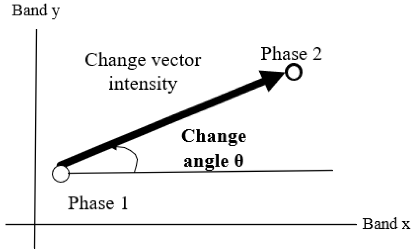Some researchers have proposed an unsupervised change detection method based on the hybrid spectral difference (HSD), which combines the spectral value and spectral shape by fusing the difference images of spectral correlation mapper (SCM) and SGD to describe the change in spectral shape [26]. One advantage of this method is that it can combine more change characteristics of the two images. One disadvantage is that many ground objects cannot be detected using a single pixel. Change vector analysis (CVA) was first used for change detection and applied to forest change [27]. This paper introduces a digital method for change detection using multi-temporal Landsat data. The method calculates the spectral change vectors of two different dates. This method works well in low-resolution images, but its disadvantage is that it only considers a single feature. Since ground objects in VHR images are more complex, applying this method to VHR remote sensing images will result in a lot of noise. To address this limitation, some researchers have proposed a change detection method that combines multiple indexes and uses CVA and SGD to construct a change difference image [28]. However, it has three disadvantages. First, although the two index algorithms are different, they both judge the changes based on image pixels. Second, although multiple index fusion can reduce part of salt and pepper noise, it still cannot use advanced features to express the whole VHR image. Third, multi-index fusion may lead to error superposition of change detection results.

In recent years, with the rapid development of various disciplines, various computer models have made outstanding progress in image processing, for example, machine learning models such as support vector machine (SVM) [29], random forest (RF) [30] and extreme learning machine (ELM) [31]. Visual saliency detection technology has also advanced in leaps and bounds, such as a spectral residual approach (SRA) [32], context-aware saliency detection (CASD) [33] and the richer convolutional features method [34]. Convolutional Neural Networks (CNN) for images have been developed in recent years, including U-Net [35], GoogleNet [36], ResNet [37], etc. These networks show strong effects in various fields of remote sensing. VHR image change detection is roughly divided into three categories. The first category is to extract the image features first and then compare them to get the change detection results. For example, some researchers have used classification CNNs, which are the main method for learning deep features from VHR remote sensing images, to detect building changes from RGB aerial photographs [38]. The second category is to use samples directly to train the change detection neural network model and then output the change image directly. For example, some researchers have used pre-trained image classification CNNs to extract change features [39]. Some researchers have used improved attention mechanisms for training networks to extract change information [40]. The third category uses some visual methods for unsupervised change detection based directly on images. For example, some researchers have proposed a base improved PCA-net model to implement VHR image change detection [41]. It exhibits an excellent performance in the field of VHR change detection. As we all know, most VHR images mainly include four bands. For remote sensing change detection, simply using these visual models to input RGB band information may cause the loss of spectral bands, thus affecting the change detection results. Therefore, it is very important to construct the correlation between remote sensing change detection algorithms and visual models.

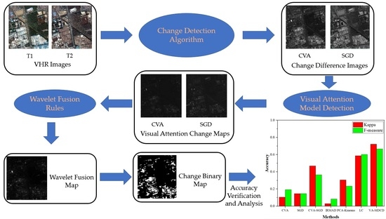
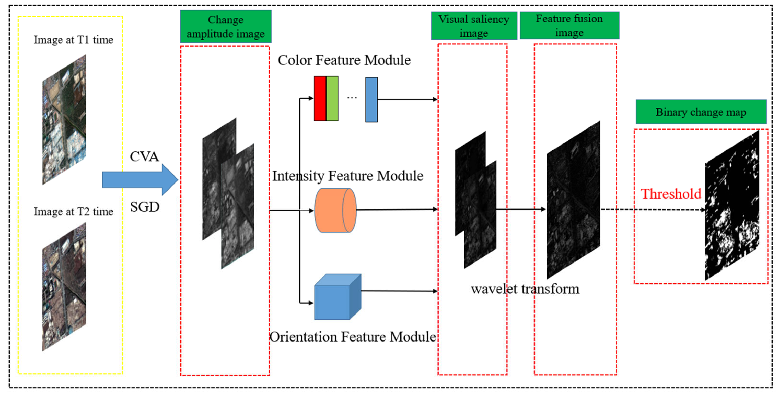
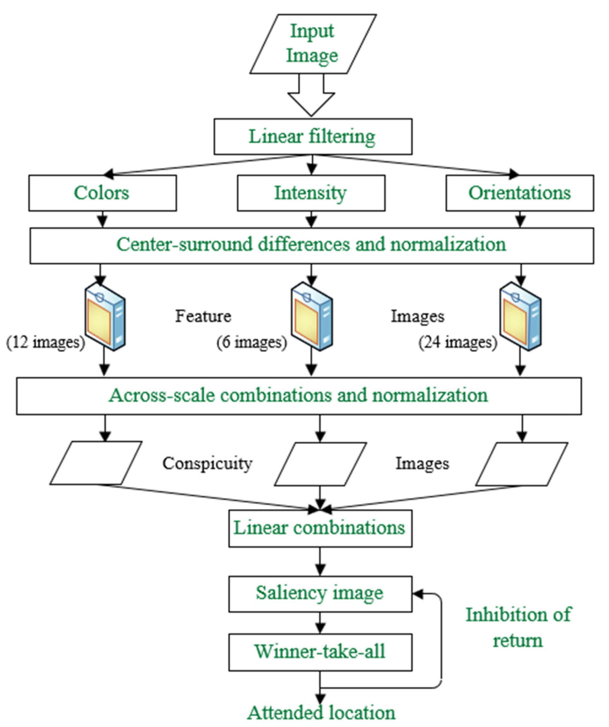
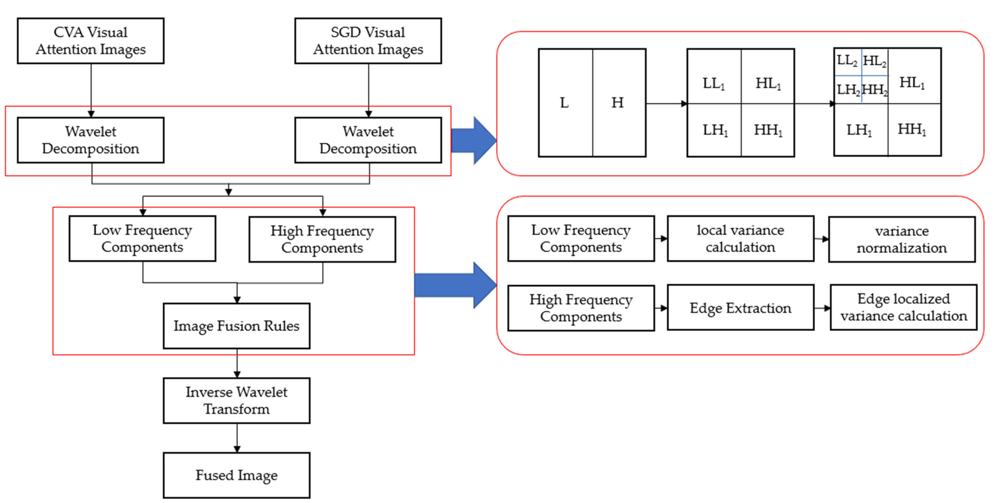
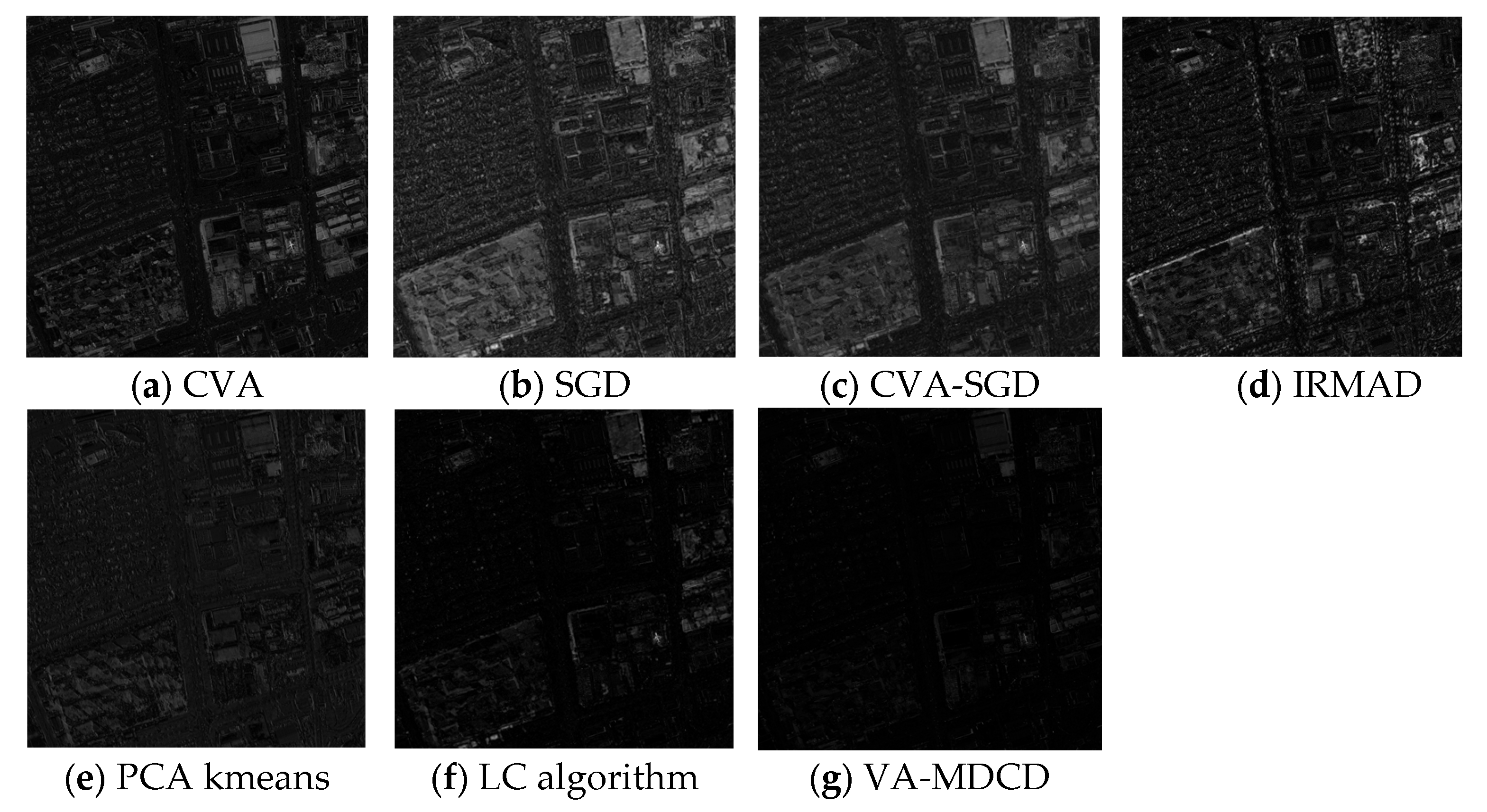
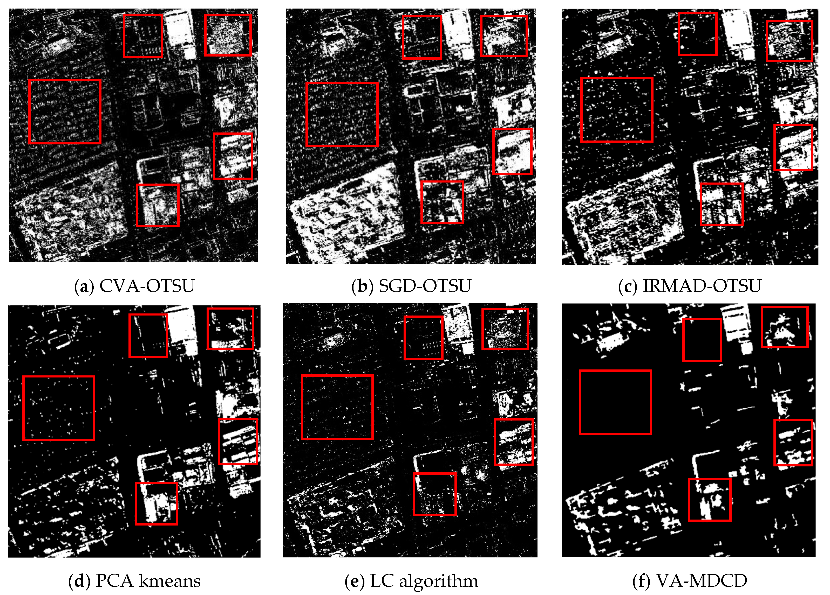
From the above analysis, it can be seen that some single feature indexes and their improved versions have different performance improvements in different aspects, but cannot express the global features of the image. The combined multi-index method does not perform well on highly complex VHR images. If a visual model is only used for VHR image change detection, the band information will be lost. Therefore, in order to overcome the problems mentioned above, we combine the visual attention model with difference image fusion and propose a multi-difference image fusion change detection algorithm based on visual attention (VA-MDCD). First, two difference images are calculated using CVA and SGD. Secondly, the two difference images are input into an Ltti visual model to calculate the color, intensity and orientation features of the images [42,43,44]. These features are combined to produce two saliency feature maps. Thirdly, a fusion result is obtained by performing the wavelet fusion algorithm [45] on two saliency feature images. Finally, the OTSU threshold segmentation algorithm (OTSU) [46] is used to obtain the change detection result. Notably, the Ltti model utilizes visual attention to enhance the efficiency and accuracy of the fusion process, providing a more robust solution for image fusion [42,43,44]. The VA-MDCD framework is designed to focus visual attention on areas of significant change. VA-MDCD can effectively combine image correlation to extract advanced features of images [47,48]. Before fusing the two indexes, VA-MDCD can significantly reduce the errors of the two indexes and focus on the real changes.

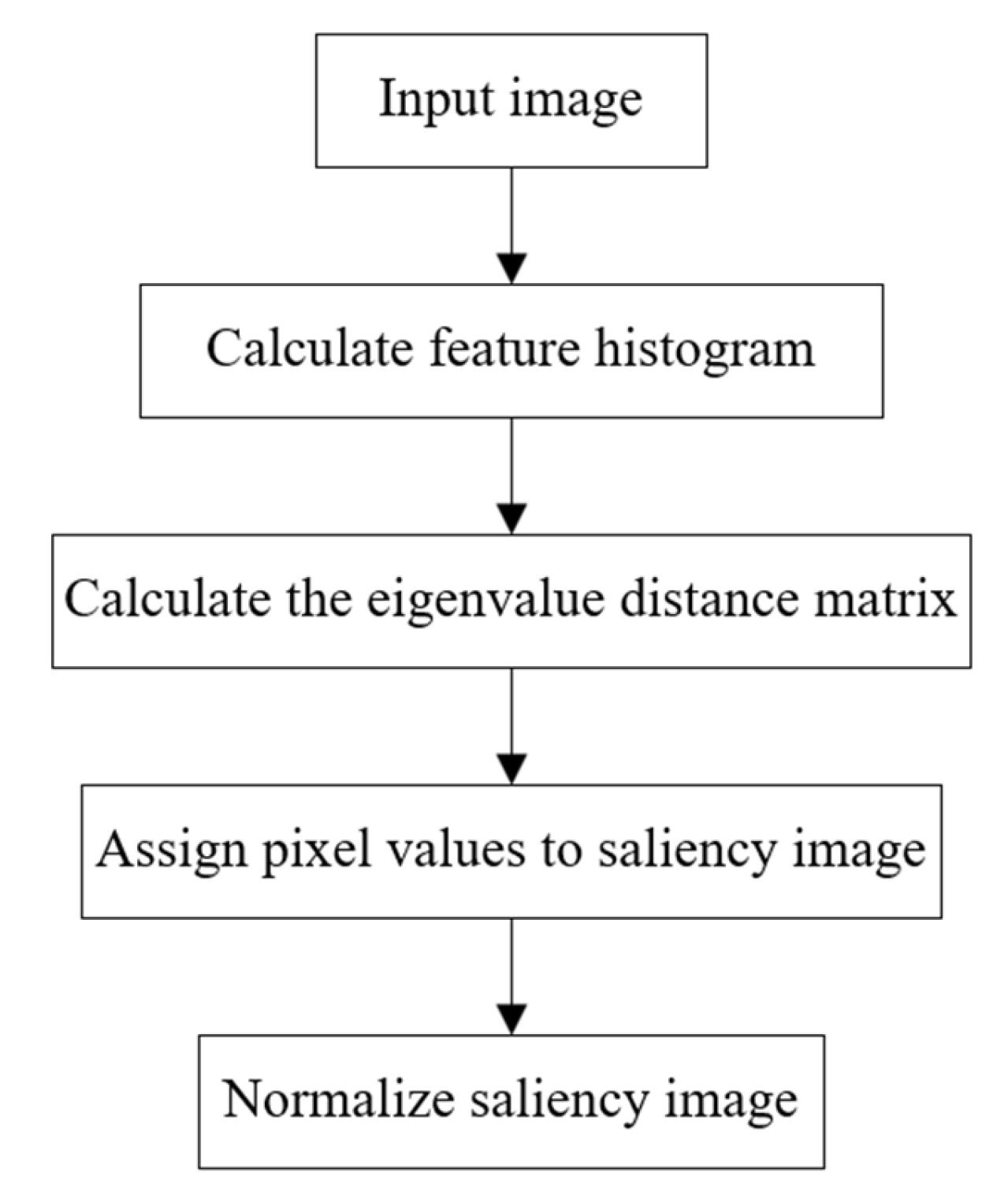
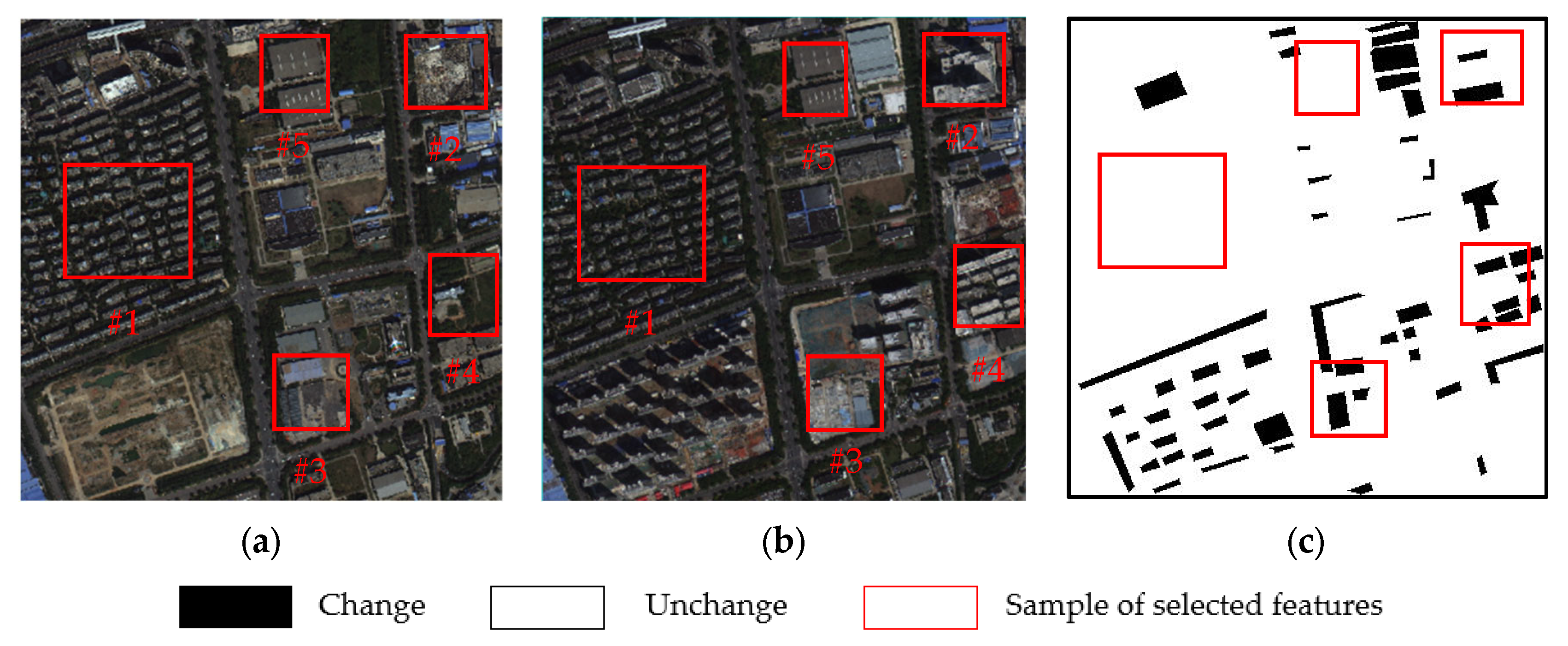
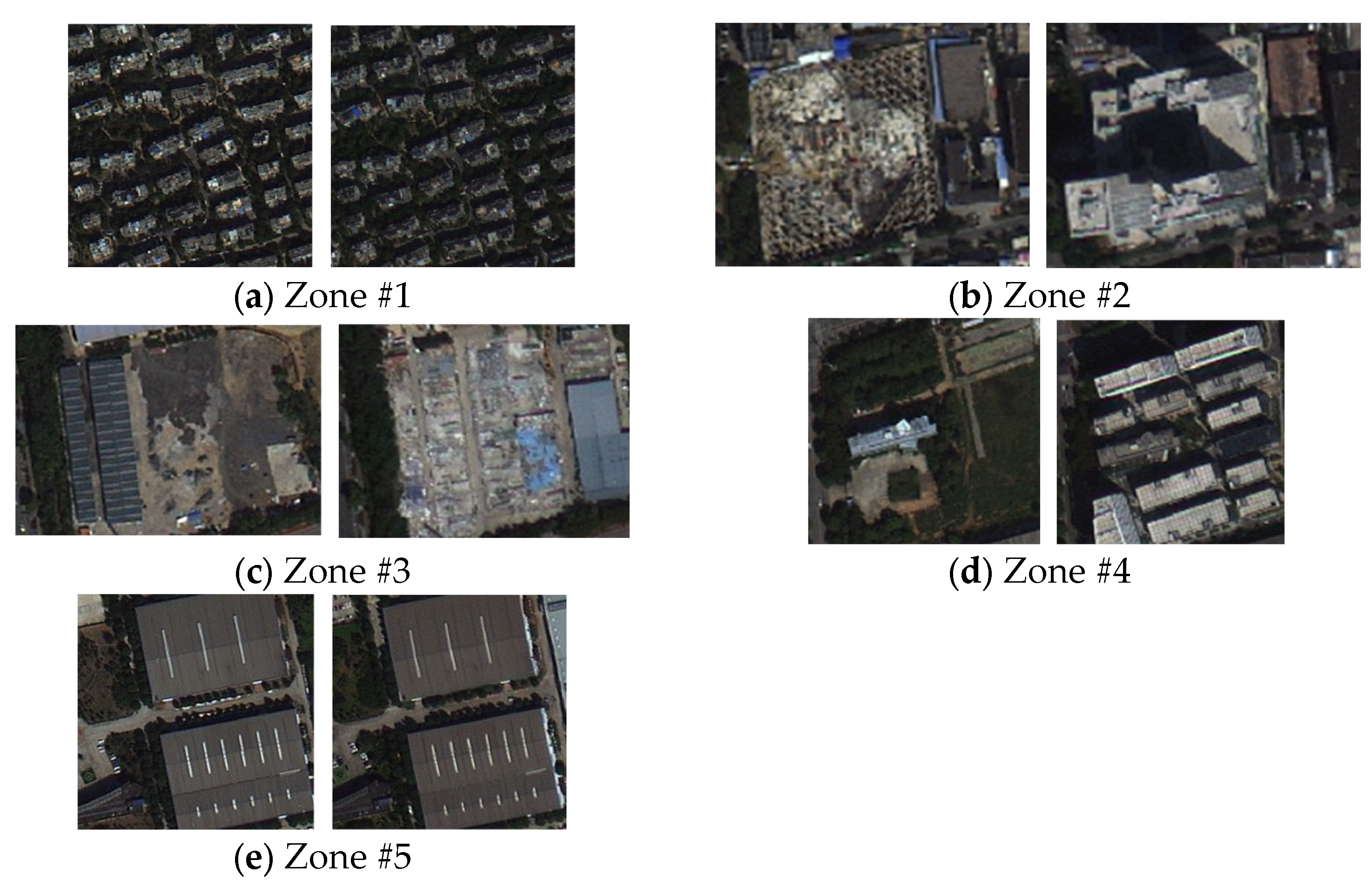
The highlights of this paper as follows: (1) a visual-attention-model-based change detection framework is proposed, which has a higher performance than the traditional multi-difference image fusion change detection method in VHR images with complex features; (2) the framework can detect changes in VHR images without the need for samples and can self-adapt to the extraction of change areas; (3) visual attention is added and a total of 42 change feature maps are computed to accurately capture changes. In total, the model has three change feature extraction modules, which compute 12 color feature maps, 6 intensity feature maps and 24 orientation feature maps (see Section 2.2.2 for specific algorithms).

In the rest of this article, Section 2 describes our proposed VA-MDCD approach and explains how to implement it. Section 3 presents our analysis of the results obtained in the two experiments. Section 4 details the design of ablation experiments to discuss the influence of different model structures on the proposed method, and Section 5 summarizes our conclusions.

2. Methods

The process of the VA-MDCD method proposed in this paper is shown in Figure 1. Firstly, we apply the CVA [27] and SGD [25] change detection algorithms to generate change amplitude images from VHR remote sensing data collected at identical locations during two distinct time periods. Secondly, we utilize a computer vision saliency algorithm to extract the saliency feature of each change amplitude image constructed by CVA and SGD, respectively. We use the Ltti model [42,43,44] for feature extraction and the Luminance Contrast (LC) algorithm [49,50] as a comparison. Thirdly, we use the wavelet transform [51] to fuse two saliency difference images. Finally, we use the OTSU algorithm to derive the binarized threshold segmentation outcomes and evaluate the change map [46].

The proposed VA-MDCD method utilizes the visual attention model to detect changes in images by leveraging color, intensity and orientation features. The fusion results represent the areas where CVA and SGD are salient together. It is also verified that this method has good detection results for complex backgrounds and complex terrain types. The specific algorithms are as follows.

2.1. Construct the Change Intensity Image

2.1.1. Change Vector Analysis

CVA [27,52] can characterize the changes in images regarding both their intensity and direction features. Figure 2 illustrates the direction and magnitude of the change vector, and we have established a separation threshold to delineate the changed and unchanged areas. Different ground objects have varying change angles, so we can classify change types according to these angles.

The principle is as follows: Set remote sensing images of phase T₁ and phase T₂ as G₁ and G₂, respectively, and pixel grey values of column j in row i are G₁ = (X_ij¹ (T₁), X_ij² (T₁), … X_ijⁿ(T₁))^T and G₂ = (X_ij¹ (T₂), X_ij²(T₂), … X_ijⁿ(T₂))^T, respectively. n is the number of selected bands and X_ij^k(T₁) is the grey value of the pixel in the T phase of column j in line i of the k band. By calculating the difference between G₁ and G₂, the change vector is obtained as follows:

$$\mathsf{\Delta }G={\mathrm{G}}_1-{\mathrm{G}}_2=\left[\begin{array}{c}{X}_{ij}{}^1(T_1)-X_{ij}{}^1(T_2)\\ X_{ij}{}^2(T_1)-X_{ij}{}^2(T_2)\\ ......................\\ X_{ij}{}^k(T_1)-X_{ij}{}^k(T_2)\\ ......................\\ X_{ij}{}^n(T_1)-X_{ij}{}^n(T_2)\end{array}\right]$$

(1)

|ΔG| is calculated from the following formula which describes information about changes in the entire image:

$$|\mathsf{\Delta }G|=\sqrt{{\displaystyle \sum _{k=1}^n{(X_{ij}{}^k(T_1)-X_{ij}{}^k(T_2))}^2}}$$

(2)

2.1.2. Spectral Gradient Difference

SGD [25] is a method that compares the spectral slope of two images captured by satellites in the same area during different time periods. The spectral slope refers to the rate at which the spectral response changes with wavelength [28].

The changing intensity of the spectral slope of the same object at the last two times can be calculated as follows:

$$Di{f}_K={\displaystyle \sum _{M=1}^N\left|\frac{(re{f}_{i,M+1}-re{f}_{j,M+1})-(re{f}_{i,M}-re{f}_{j,M})}{{\rho }^{’}{}_{M+1}-{\rho }^{’}{}_M}\right|}$$

(3)

In this formula, ref_i,M+1 is the spectral brightness value of the M + 1 band in the T₁ phase, ref_i,M is the spectral brightness value of the M band, ref_j,M+1 is the spectral brightness value of the M + 1 band in the T₂ phase, and ref_j,M is the spectral brightness values of the M band. ρ^’_M+1 and ρ^’_M are the normalized wavelengths of the corresponding bands and Dif_K is the change intensity of the two slope vectors. The larger the value, the more likely the surface cover will change in the area; otherwise, the probability is lower. Finally, it is necessary to set a threshold to determine whether there is a change.

2.2. Visual Attention Model

The Ltti model is a computer vision attention model [42,43,44]. In this model, three kinds of features are used to represent the image, which are color, intensity and orientation. The model is shown in Figure 3. Firstly, feature pyramids are constructed. Secondly, feature images are calculated. Finally, visual saliency images are calculated.

2.2.1. Feature Extraction

An intensity image I is I = (r + g + b)/3, where r, g and b are the red, green and blue channels of the input image. I is used to create a Gaussian pyramid I(σ), where σ ∈ [0...8] is the scale. The four color channels are R = r − (g + b)/2 for red, G = g − (r + b)/2 for green, B = b − (r + g)/2 for blue and Y = (r + g)/2 − |r − g|/2 − b for yellow. Four Gaussian pyramids, R(σ), G(σ), B(σ) and Y(σ), are created from these color channels [53,54].

2.2.2. Feature Image

All features are calculated using a set of methods called center–surround methods (Figure 3). The center is c ∈ {2,3,4} and the surround is s = c + d, where d ∈ {3,4}. The center and surround values are used to derive the feature image:

$$\left\{\begin{array}{l}I(c,s)=\left|I(c)\mathrm{\Theta }I(s)\right|\\ RG(c,s)=\left|(R(c)-G(c))\mathrm{\Theta }(G(s)-R(s))\right|\\ BY(c,s)=\left|(B(c)-Y(c))\mathrm{\Theta }(Y(s)-B(s))\right|\\ O(c,s,\theta )=\left|O(c,\theta )\mathrm{\Theta }O(s,\theta )\right|\end{array}\right.$$

(4)

In the above formula, I (c, s) is the intensity feature. Above, Θ represents interpolating a coarse scale to a fine scale and subtracting matrix elements. RG (c, s) and BY (c, s) are used to represent color features. O (c, s, θ) is the orientation feature image, which is generated by comparing the orientation information between the center and surround scales, where the value range of θ is θ ∈ {0°, 45°, 90°, 135°}. A total of 6 intensity features, 12 color features and 24 orientation features were calculated.

2.2.3. Saliency Image

Saliency images are computed on a scale of 4, with $\overline{I}$ representing intensity, $\overline{C}$ representing color and $\overline{O}$ representing orientation. ⊕ represents cross-scale addition:

$$\left\{\begin{array}{l}\overline{I}=\underset{c=2}{\overset{4}{\oplus }}\underset{s=c+3}{\overset{c+4}{\oplus }}N(I(c,s))\\ \overline{C}=\underset{c=2}{\overset{4}{\oplus }}\underset{s=c+3}{\overset{c+4}{\oplus }}[N(RG(c,s))+N(BY(c,s))]\end{array}\right.$$

(5)

The four orientation values are combined together to obtain the following orientation saliency image:

$$\overline{O}={\displaystyle \sum _{\theta \in \{0^{\mathrm{o}},{45}^{\mathrm{o}},{90}^{\mathrm{o}},{135}^{\mathrm{o}}\}}N(}\underset{c=2}{\overset{4}{\oplus }}\underset{s=c+3}{\overset{c+4}{\oplus }}N(O(c,s,\theta )))$$

(6)

The overall saliency image S is:

$$S=\frac{1}{3}(N(\overline{I})+N(\overline{C})+N(\overline{O}))$$

(7)

2.3. LC Saliency Detection Algorithm

Figure 4 shows the steps of the LC algorithm [49,50].

To calculate the distinct value of a pixel in an image, we compute its global contrast in the entire image. The saliency value of pixels can be obtained using the following formula:

$$SalS(I_k)={\displaystyle \sum _{\forall I_i\in I}|I_k}-I_i|$$

(8)

In this formula, I_k represents the grey value of pixel k, I_i represents all pixel points, where the value range of i is [1, N], and SalS(I_k) represents the significant value of pixel k.

2.4. Difference Feature Fusion and Segmentation

Figure 5 shows the wavelet fusion method. We establish a wavelet pyramid decomposition of the image by applying the wavelet transform to the saliency image. Then, we fuse the decomposition layers from high to low by using different fusion rules to combine different frequency components in each decomposition layer. Finally, we obtain a fused wavelet pyramid by performing the wavelet inverse transform on the fused pyramid. The resulting image after reconstruction is the fused image [51]. In addition to this, in the process of wavelet decomposition, L and H stand for low and high frequencies, respectively. The subscripts 1 and 2 represent the first and second level decompositions, and at each decomposition level, the image is decomposed into four frequency bands in vertical and horizontal directions. In addition to this, in the process of wavelet decomposition, L and H stand for low and high frequencies, respectively. The subscripts 1 and 2 represent the first and second level decompositions, and at each decomposition level, the image is decomposed into four frequency bands in the vertical and horizontal directions. In the wavelet fusion process, low frequencies are directly fused using local variance normalization, while high frequencies are first calculated by the Canny operator to compute the edge information, and then the local variance is computed [55,56].

2.4.1. Wavelet Decomposition

The basic principle of the wavelet transform is that L layer wavelet decomposition is carried out to obtain the 3L + 1 layer frequency band, including the low frequency baseband C_j and the high frequency sub-band Dh, Dv, Dd of layer 3L. The original image is represented by f (x, y), denoted by C₀. If the filter coefficient matrix corresponding to the scale coefficient and the wavelet coefficient are H and G, respectively, then the two-dimensional wavelet decomposition algorithm can be described as follows:

$$\left\{\begin{array}{l}{C}_{j+1}=H{C}_j{H}^T\\ D_{j+1}^h=G{C}_j{H}^T\\ D_{j+1}^v=H{C}_j{G}^T\\ D_{j+1}^d=G{C}_j{G}^T\end{array}\right.$$

(9)

where j represents the number of decomposition layers; h, v and d represent horizontal, vertical and diagonal directions, respectively; and H^T and G^T are conjugate transpose matrices of H and G, respectively.

2.4.2. Wavelet Fusion

After wavelet decomposition, the low frequency part of the image is the overview and average characteristics of the image and the high frequency part of the image reflects the details of the image, such as the edge of the image, and regional boundaries. Assuming that the low-frequency components are AA and AB, the local variance Var (i, j) AA and Var (i, j) AB of all pixels of AA and AB is calculated and normalized. Then, the normalized local variance is used for low-frequency fusion. Assuming that the high-frequency components of images A and B are DLA and DLB, the edge of each high-frequency component is extracted by the Canny operator, then the local variance of each element of the edge image is calculated. The high-frequency coefficient that represents the lth layer of the source image processed by the Canny operator is the average value of the lth layer of the source image extracted by the Canny operator, which is the local variance obtained by edge extraction of the high-frequency component of the lth layer of the source image. Then, the fused coefficient is reconstructed by a wavelet to obtain the fused image.

The low frequency fusion adopted in this paper adopts the fusion rule of mean square deviation normalization, and the high frequency fusion adopts the Canny operator for edge extraction. The local variance of each pixel is calculated because the high-frequency part is the edge area of the image, so this method is used. The Canny edge detection algorithm is a classic edge detection algorithm used to extract the edge of the image to better highlight high-frequency features.

2.4.3. OTSU Threshold Segmentation Algorithm

After difference image fusion, we use the OTSU [46] segmentation algorithm for image binarization. C₀ and C₁ are two classes whose pixel values have intervals of [1, …, T] and [T + 1, …, L], respectively, with T being the given critical value. σ_b²(T) and σ_w²(T) represent inter-class variance and intra-class variance, respectively, and the threshold of variance is:

$$T^{*}=\underset{1\le T<L}{\arg }\max \{{\sigma }_b^2(T)\}=\underset{1\le T<L}{\arg }\min \{{\sigma }_w^2(T)\}$$

(10)

3. Results

To validate the effectiveness of VA-MDCD, we selected two datasets for two experiments. The first dataset was two images taken by the Jilin-1 (JL-1) satellite [57]. The second dataset was two images taken by the Beijing-2 (BJ-2) satellite [58]. Both datasets include multispectral and panchromatic imagery. Before executing our algorithm framework, both datasets underwent precise preprocessing procedures. Firstly, the multispectral imagery underwent radiometric calibration, atmospheric correction and orthorectification. Secondly, the panchromatic imagery was subjected to radiometric calibration and orthorectification. Radiometric calibration was performed to eliminate interference from the sensor itself, the atmosphere, the solar zenith angle and terrain effects. Atmospheric correction was applied to effectively mitigate errors caused by atmospheric scattering, absorption and reflection. Orthorectification was conducted to bring the two temporal images closer to the orthorectified angle. Subsequently, the preprocessed multispectral and panchromatic images were fused using the Gram–Schmidt (G–S) algorithm [59]. Importantly, we finally performed geometric registration on the processed images at different times to ensure the correspondence of pixels between the two images. The land cover types of both images in the JL-1 dataset only included vegetation and impervious surface, while the images in the BJ-2 dataset only included impervious surface.

3.1. Experiment #1

3.1.1. Experimental Data

We have selected JL-1 VHR images as the data of experiment 1. JL-1 satellite remote sensing images have been successfully applied in urban streetlight extraction, surface water resources monitoring, forest ignition recognition, urban real-time traffic monitoring and others. The resolution of panchromatic images taken by the satellite is 0.72 m, and the resolution of multispectral images is 2.88 m. The JL-1 image pair was acquired in October 2018 and November 2019.

3.1.2. Change Detection Results and Statistical Analysis

The images have been cut to 1915 × 2101 pixels in the red, green, blue and near-infrared regions. The cropped images are shown in Figure 6. A reference change image was obtained through detailed field investigations and unmanned aerial vehicle (UAV) measurements, so the visual analysis has some prior knowledge. The black part is the actual change area.

In order to evaluate the improvements in the VA-MDCD method on multiple difference image fusion, five pairs of error-prone ground objects marked with red rectangles in the original image were selected as samples for analysis (Figure 7). The spectra of zones #1, 2, 6 and 7 changed in the two images, but they cannot be considered changed. Zones #3, 4 and 5 are vulnerable to rain erosion and cause false detections. They were therefore selected as samples for analysis.

All experiments were conducted under the same computer environment. To compare with this experiment and verify the reliability of this experiment, in addition to the proposed VA-MDCD method and LC algorithm, another five groups of comparison experiments were designed: the change results of the combination of CVA [27] and OTSU algorithms (CVA-OTSU); the change results of the combination of SGD [25] and OTSU (SGD-OTSU); the change results of CVA-SGD [28] fusion; iterative weighted multivariate [60] change detection (IRMAD-OTSU); and change detection based on PCA kmeans [61] (PCA kmeans). Figure 8a–g shows the change amplitude images of CVA, SGD, CVA-SGD, IRMAD, PCA kmeans, LC algorithm and VA-MDCD, respectively. From VA-MDCD, we can see that our method can well suppress most of the salt-and-pepper noise and spurious changes in CVA and SGD. Influenced by visual attention, our method is closer to human vision, and the magnitude of VA-MDCD changes is closer to the real changes. The change detection results are shown in Figure 9, where the white area is the changed area and the black area is the unchanged area.

3.1.3. Analysis and Discussion

A confusion matrix was introduced here to evaluate the accuracy. The overall accuracy (OA), false alarm rate (FA), missed alarm rate (MA), Kappa and F-measure were calculated using the confusion matrix, and the experimental results were quantitatively analyzed and evaluated by these coefficients [62].

The OA is the ratio of all correctly classified samples to total samples. The formula is as follows:

$$OA=\frac{TP+TN}{TP+TN+FP+FN}$$

(11)

where TP and TN represent the number of pixels that are actually changed and correctly detected as changed and the number of pixels that are actually unchanged and correctly detected as unchanged, respectively. FP and FN represent the number of pixels that are actually changed but incorrectly detected as unchanged and the number of pixels that are actually unchanged but incorrectly detected as changed, respectively. FA represents the ratio of the unchanged area detected as the changed area to the true unchanged area:

$$FA=\frac{FP}{FP+TN}$$

(12)

MA represents the ratio of the undetected area of change to the actual area of change:

$$MA=\frac{FN}{FN+TP}$$

(13)

Kappa is used to test the consistency of the results. The higher the Kappa value, the more accurate the result. The formula is as follows:

$$Kappa=\frac{(OA-PRE)}{(1-PRE)}$$

(14)

In this formula, PRE represents the consistent rate of the theoretical test results. The formula is as follows:

$$PRE=\frac{(TP+FP)(TP+FN)+(TN+FN)(TN+FP)}{{(TP+TN+FN+FP)}^2}$$

(15)

The F-measure coefficient is the arithmetic mean divided by the geometric mean; the larger the value, the more accurate the final change detection results. The formula is as follows:

$$F-measure=\frac{T{P}^2}{T{P}^2+FN+FP}$$

(16)

According to the accuracy evaluation table (

Table 1. The accuracy table of different change detection methods.

Methods	OA (%)	FA (%)	MA (%)	Kappa	F-Measure
CVA-OTSU	83.47	19.53	23.56	0.1055	0.1922
SGD-OTSU	79.55	26.45	20.22	0.1472	0.1460
CVA-SGD	89.36	17.16	22.47	0.4683	0.3645
IRMAD-OTSU	80.41	30.72	35.34	0.0291	0.0842
PCA kmeans	86.25	13.29	25.92	0.3056	0.2336
LC algorithm	91.54	11.74	27.36	0.5874	0.6018
VA-MDCD	94.50	8.59	23.28	0.7228	0.6671

) and the visualization results in Figure 10, the proposed VA-MDCD had a higher OA, Kappa and F-measure than other comparison methods. For VA-MDCD, they were 94.50%, 72.28% and 66.71%, respectively, and for the LC algorithm, they were 91.54%, 58.74% and 60.18%, respectively. The direct fusion of CVA and SGD could not distinguish spurious changes caused by different sun angles. It should be noted that there were still some noise and spurious variations in the proposed VA-MDCD, which slightly affected the accuracy. In general, based on the analysis of accuracy, we conclude that the VA-MDCD method proposed in this paper is effective and reliable. Furthermore, the FA of the proposed VA-MDCD was 8.59%, which was reduced by 8.57% compared to CVA-SGD. Although the proposed method falsely detected some building shadows, it could reduce the effect of CVA and SGD fusion errors.

Table 2. The number of pixels per sample.

Value	Zone #1	Zone #2	Zone #3	Zone #4	Zone #5	Zone #6	Zone #7
Number of pixels	92,880	61,180	60,532	56,225	6936	40,000	62,500

counts the pixel number of the selected five pairs of sample areas, and

Table 3. Number of pixels for error detection of each sample by different methods.

	Zone	CVA	SGD	CVA-SGD	VA-MDCD
Pixel value for error detection	Zone #1	541	977	1291	134
	Zone #2	3421	23,823	13,269	0
	Zone #3	25,816	51,185	18,571	1323
	Zone #4	24,594	41,272	29,533	397
	Zone #5	3213	1924	3918	552
	Zone #6	17,327	21,928	3635	0
	Zone #7	19,483	35,167	41,368	1451

details the false detection pixels of five pairs of samples by CVA, SGD, CVA-SGD and VA-MDCD. In Table 3, the number of false detection pixels of CVA-SGD was higher than that of CVA and SGD, and some were between CVA and SGD, but none of them had a reduced number of false detection pixels. Although the results of the VA-MDCD method also had a lot of pixel misdetection, compared with CVA-SGD, it could effectively improve the fusion effect of CVA and SGD. Although the FA of CVA-SGD was lower than that of both CVA and SGD, the number of misdetected pixels in specific areas was very high. The proposed VA-MDCD method reduced the total FA and the number of misdetected pixels in specific areas. The spectra of these features in zones #1, #2, #6 and #7 have changed, and we cannot actually consider them as changed zones, so there are only very few erroneous pixels in the VA-MDCD results, which proves that our method is able to remove spurious changes due to spectral effects very well.

3.2. Experiment #2

3.2.1. Experimental Data

We have selected BJ-2 VHR images as the data for experiment 2. The satellite consists of three optical remote sensing satellites in the 0.8 m panchromatic band and 3.2 m multi-spectral band, which can provide high-quality remote sensing images. The BJ-2 image pair was acquired in October 2018 and September 2021.

3.2.2. Change Detection Results and Statistical Analysis

The images were cut to 1500 × 1500 pixels in the red, green, blue and near-infrared regions. The cropped image is shown in Figure 11. A reference change detection image was obtained by visual interpretation and geographic analysis, and the black part is the actual changed area.

In experiment 2, we used red rectangles to select four pairs of ground objects in the original image that were easily affected by the shooting angle of the sensor (Figure 12).

All experiments were conducted under the same computer environment. To compare with this experiment and verify the reliability of this experiment, in addition to the proposed VA-MDCD method and LC algorithm, another five groups of comparison experiments were designed. The five methods are CVA [27], SGD [25], CVA-SGD [28], IRMAD [60] and PCA kmeans [61]. Figure 13a–g presents the change amplitude images of CVA, SGD, CVA-SGD, IRMAD, PCA kmeans, LC algorithm and VA-MDCD, respectively. From VA-MDCD, we can see that our method effectively suppresses the majority of salt-and-pepper noise and spurious changes, such as urban rooftops. VA-MDCD efficiently focuses attention on areas with salient changes. The change detection results are shown in Figure 14; the white area is the changed area and the black area is the unchanged area.

3.2.3. Analysis and Discussion

According to the accuracy evaluation table (

Table 4. The accuracy table of different change detection methods.

Methods	OA (%)	FA (%)	MA (%)	Kappa	F-Measure
CVA-OTSU	85.24	21.36	24.75	0.2258	0.1226
SGD-OTSU	86.58	18.94	17.39	0.1326	0.1865
CVA-SGD	90.21	15.75	22.65	0.5758	0.4903
IRMAD-OTSU	84.92	24.13	21.87	0.3714	0.2642
PCA kmeans	88.76	14.92	26.17	0.3940	0.2036
LC algorithm	91.02	12.76	25.63	0.5981	0.5487
VA-MDCD	94.74	6.19	18.94	0.8422	0.7313

) and the visualization results in Figure 15, the proposed VA-MDCD had a higher OA, Kappa and F-measure than other comparison methods. For VA-MDCD, they were 94.74%, 84.22% and 73.13%, respectively, and for the LC algorithm, they were 91.02%, 59.81% and 54.87%, respectively. In this verification area, the direct fusion method of CVA and SGD could not distinguish the errors caused by different sensor tilt angles. It was worth noting that there was still a small number of false detections in the proposed method, which slightly affected the accuracy of change detection. Overall, based on a quantitative analysis of the results, the FA of the proposed method was 6.19%, which was reduced by 9.56% compared to CVA-SGD. We conclude that the proposed VA-MDCD method is also reliable for quasi-urban area detection, and the proposed VA-MDCD can reduce the fusion error of CVA and SGD.

Table 5. The number of pixels per sample.

Value	Zone #1	Zone #2	Zone #3	Zone #4	Zone #5
Number of pixels	80,089	26,070	21,879	22,194	32,400

and

Table 6. Number of pixels for error detection of each sample by different methods.

	Zone	CVA	SGD	CVA-SGD	VA-MDCD
Pixel value for error detection	Zone #1	26,323	34,674	27,338	0
	Zone #2	9821	7334	14,935	652
	Zone #3	10,372	16,038	15,973	243
	Zone #4	3679	5614	6385	465
	Zone #5	8154	6012	7305	0

, respectively, show the total pixel values of the four pairs of samples and the number of misdetected pixels of CVA, SGD, CVA-SGD and VA-MDCD. Table 6 shows that the proposed VA-MDCD can effectively improve the fusion result of CVA and SGD. Among the four samples, the VA-MDCD method produced a low number of false detection pixels, and one sample even had 0. Although the overall effect CVA-SGD was better than CVA and SGD, it was less effective in some details. Therefore, we conclude that CVA-SGD can remove a lot of noise on the whole. However, because CVA-SGD only calculates spectral features, it could not represent the information of the whole image, so it was not effective to apply it to the VHR image. The proposed VA-MDCD could combine multiple features to effectively improve the performance of CVA-SGD applied to VHR images. It is worth noting that in zones #1 and 5 there is no change in the building morphology. Due to the spectral changes on the roofs, CVA, SGD and CVA-SGD would have detected them as areas of change, which is incorrect. However, VA-MDCD avoids this spurious change by integrating spatial correlation. Therefore, VA-MDCD has a strong performance in solving the problem of spurious changes due to spectral effects.

In general, both CVA and SGD could cause false detections on VHR images. CVA-SGD exhibited a slightly better performance compared to CVA and SGD, with a higher OA. However, noise remained present, and CVA-SGD did not eliminate the error accumulation of CVA and SGD in certain regions. In the results of IRMAD, both FA and MA were very high, with numerous errors and significant salt-and-pepper noise. This phenomenon shows that it is not feasible to use spectral features only in VHR images. Due to the consideration of contextual information in the image, PCA kmeans reduced the noise to some extent, but the performance was not efficient. Although the method combined with the LC algorithm eliminated some noise, the overall effect was not good. The reason was that the LC algorithm only calculated the contrast features of the image, which could not fully express the relationship between the pixels of the entire image. VA-MDCD not only had a good detection effect on VHR images, but also eliminated a lot of noise and low building shadows and could reduce the error superposition after the fusion of CVA and SGD, which was especially obvious. It was worth noting that the proposed VA-MDCD did not eliminate the shadows caused by tall buildings. The most important point is that the algorithm framework we designed is unsupervised, which can achieve good change detection results without any samples. Traditional algorithms are mostly unsupervised algorithms. Our algorithm performs better than traditional unsupervised algorithms, and it can be applied to VHR images. Therefore, the novelty of our algorithm is reflected here.

4. Discussion

4.1. Effect of Different Model Structures

As we all know, the combination of a computer vision algorithm and a change detection algorithm involves multiple processes, and each stage has uncertainty. We need to design experiments to justify the use of different modules to highlight the benefits of using different modules in the proposed method. We divided the model structure of the proposed method and designed ablation experiments to verify the influence of the color, intensity and orientation modules on the change detection results.

In addition to the proposed methods, the ablation experiments also include methods without color modules, methods without intensity modules and methods without orientation modules. The specific experimental results are summarized in Section 4.2.

4.2. Ablation Experiments

The change detection results of the designed experiment on the two datasets are shown in Figure 16. Here, the two datasets are named A and B. As can be seen from the results figure, the results of VA-MDCD show a good detection effect compared with the results with any of the three modules missing, and the textural structure is clear and the fragmented noise processing is better.

In addition, we also counted the F-measure values of the results generated by all model structures. The statistical figure is shown in Figure 17. It can be seen that the F-measure value and performance of the proposed VA-MDCD were higher than those produced by the other three model structures regardless of dataset. In dataset A, VA-MDCD improved by 6.33%, 1.18% and 4.41% compared to not using a color module, intensity module or orientation module, respectively. In dataset B, VAMDCD improved by 15.89%, 7.34% and 4.09% compared to not using a color module, intensity module or orientation module, respectively. The color module had the greatest impact on both datasets, since color plays the most important role in the magnitude image. VA-MDCD was affected by the lack of any kind of module, which indicates that the three feature extraction modules introduced can help improve the performance of VHR image change detection.

4.3. Comparison with Other Visual Saliency Models

To prove the effectiveness of the proposed method, we compared our method with two other commonly used visual saliency models. They are the Luminance Contrast [63,64] (LC) method and Spectral Residual (SR) method [32,65]. The LC algorithm is an effective method to calculate a spatial saliency map using image color statistics. The algorithm takes into account the computational linear complexity in the number of image pixels. A saliency map of an image is built on the grayscale contrast between image pixels. That is, the sum of the gray value distances between the pixel and all the pixels in the image is taken as the significance value of the pixel. The SR algorithm extracts and emphasizes high-frequency information by transforming the image in the frequency domain and calculating the spectral residue and regards it as salient information.

Figure 18 shows the change detection results of different selected visual saliency models, and

Table 7. F-measure values and running times of different visual saliency models.

Dataset	Model	F-Measure	Running Time (s)
A	LC algorithm	0.6018	73.14
	SR algorithm	0.6114	83.12
	Proposed VA-MDCD	0.6671	135.24
B	LC algorithm	0.5487	54.28
	SR algorithm	0.6003	71.06
	Proposed VA-MDCD	0.7313	103.48

shows the F-measure accuracy and running time of these models. From this, we can see that both LC algorithm and SR algorithm, although their running time is very short, can quickly detect the target area, but they have not eliminated the impact of noise and there are still many false changes. The LC algorithm only includes the relationship between the contrast of each pixel. Although the SR algorithm can be used to quickly calculate the significant region in the image, it may have some limitations in complex scenes, such as an insensitivity to color information and a limited ability to process images with complex backgrounds. Therefore, in relatively complex scenes, our method mimics human vision and combines multi-scale visual features to achieve more effective change detection results.

4.4. Model Complexity

In order to comprehensively evaluate the performance of the proposed framework, we need to compute statistics on the hardware facilities and computing time of the computer. In addition, we also need to evaluate the number of parameters of the whole model. Here, all experiments were conducted on all datasets and all experiments were conducted on an Intel Core i7-11800H CPU @ 2.3 GHz (16 GB RAM) with a NVIDIA GeForce Experience 3060 GPU. The model we developed was mainly implemented in matlab2019b and all the parameters and variables can be debugged on matlab2019b.

Table 8. The number of running parameters of different model structures and the running time of all methods on the two datasets A and B.

Dataset	Model Structure	Number of Running Parameters (k)	Running Time (s)
A	CVA	-	3.21
	SGD	-	2.94
	CVA-SGD	-	6.53
	IRMAD	-	1.79
	LC algorithm	-	73.14
	PCA kmeans	-	49.25
	without color	25.11	126.91
	without intensity	23.45	127.25
	without orientation	20.74	113.93
	VA-MDCD	26.32	135.24
B	CVA	-	2.67
	SGD	-	2.14
	CVA-SGD	-	5.33
	IRMAD	-	1.74
	LC algorithm	-	54.28
	PCA kmeans	-	39.58
	without color	25.11	88.72
	without intensity	23.45	97.86
	without orientation	20.74	87.25
	VA-MDCD	26.32	103.48

shows the running time and parameter number statistics of the different structural models. In addition, the algorithm running times of the comparison experiment in Section 3 are also listed. It can be seen from the table that the proposed VA-MDCD has more running parameters and takes more time than other models, but this increase can be ignored, which is worthwhile compared with the improvement in the performance of change detection.

5. Conclusions

The introduction of this paper summarized the limitations of conventional techniques while suggesting new approaches to overcome these shortcomings. We proposed a novel approach to detect changes in remote sensing images using an attention model in computer vision, which has been called VA-MDCD.

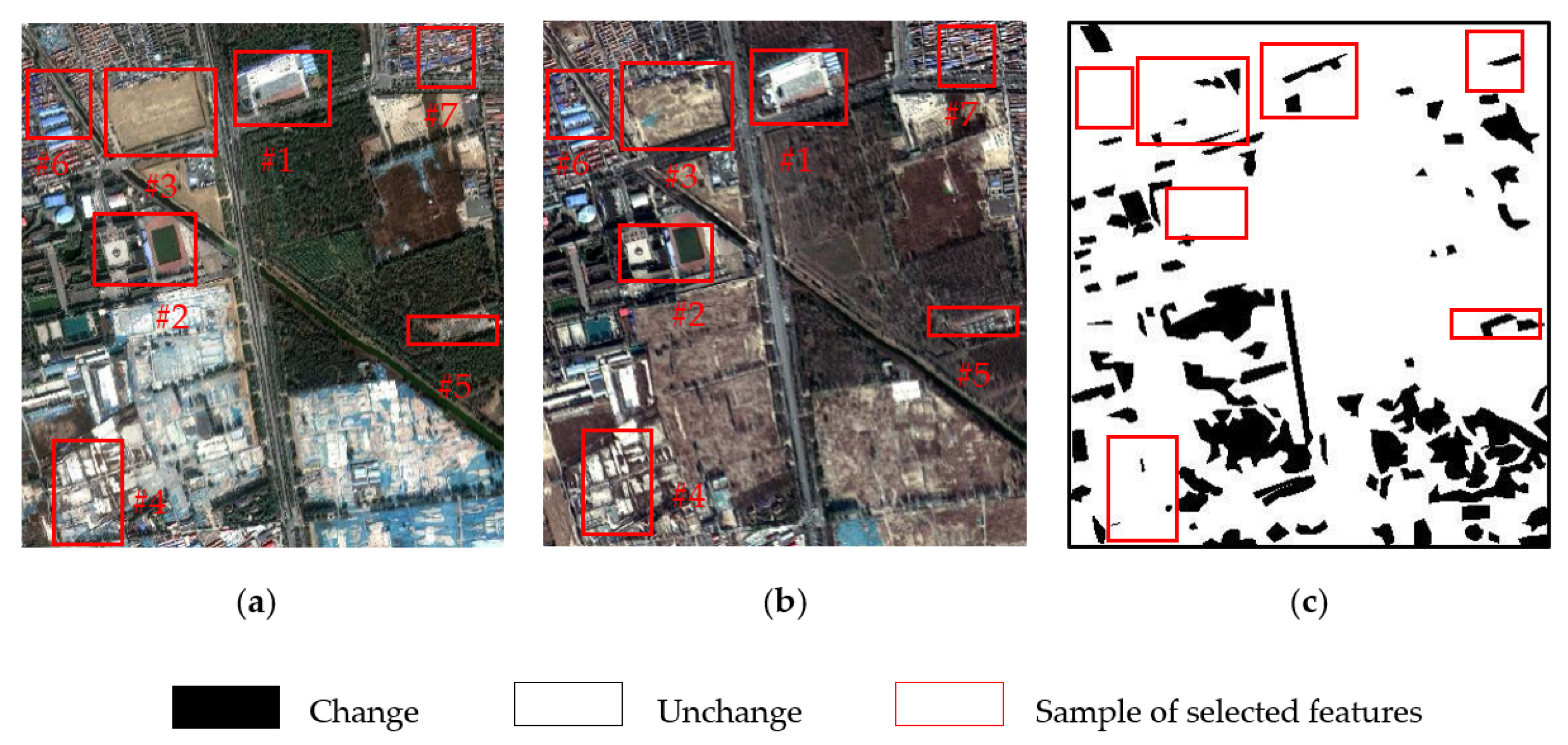
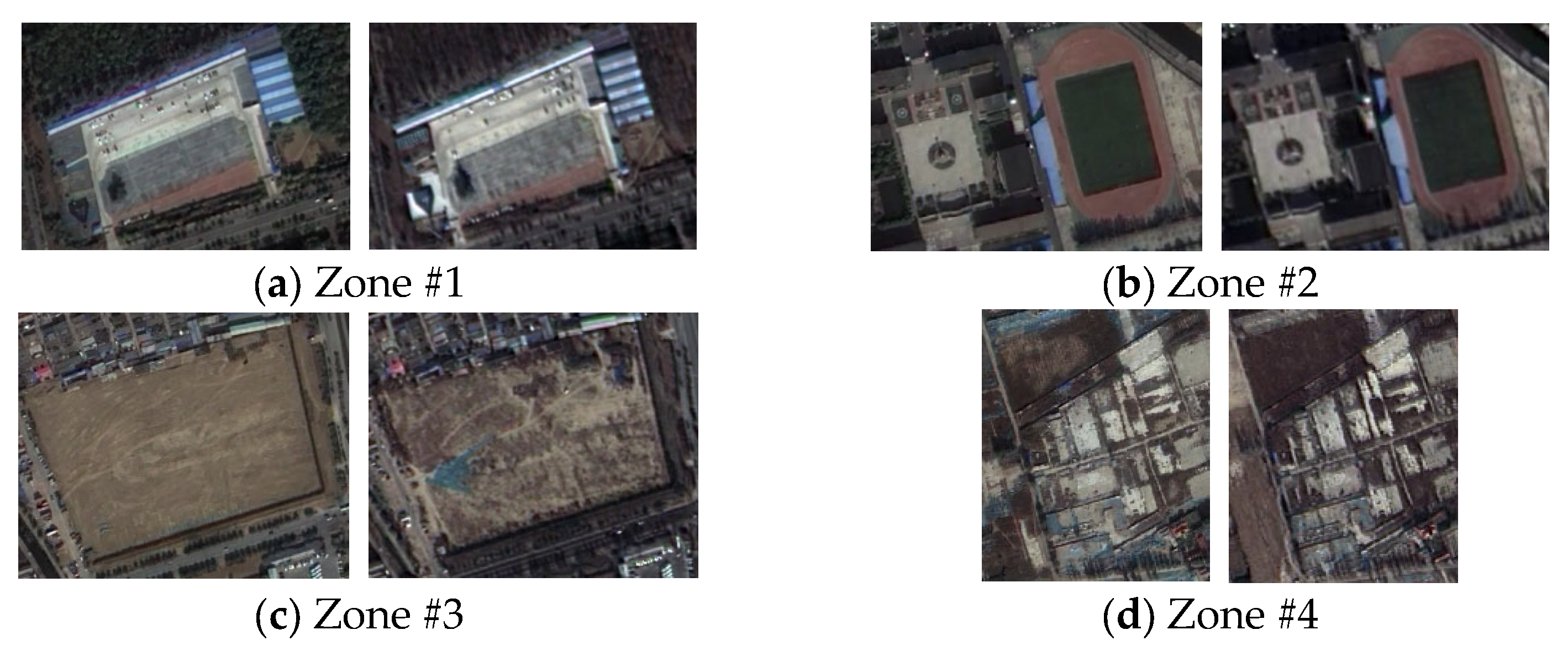
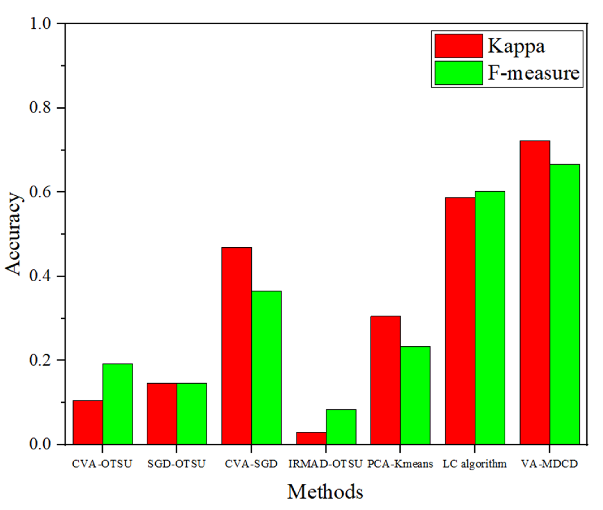
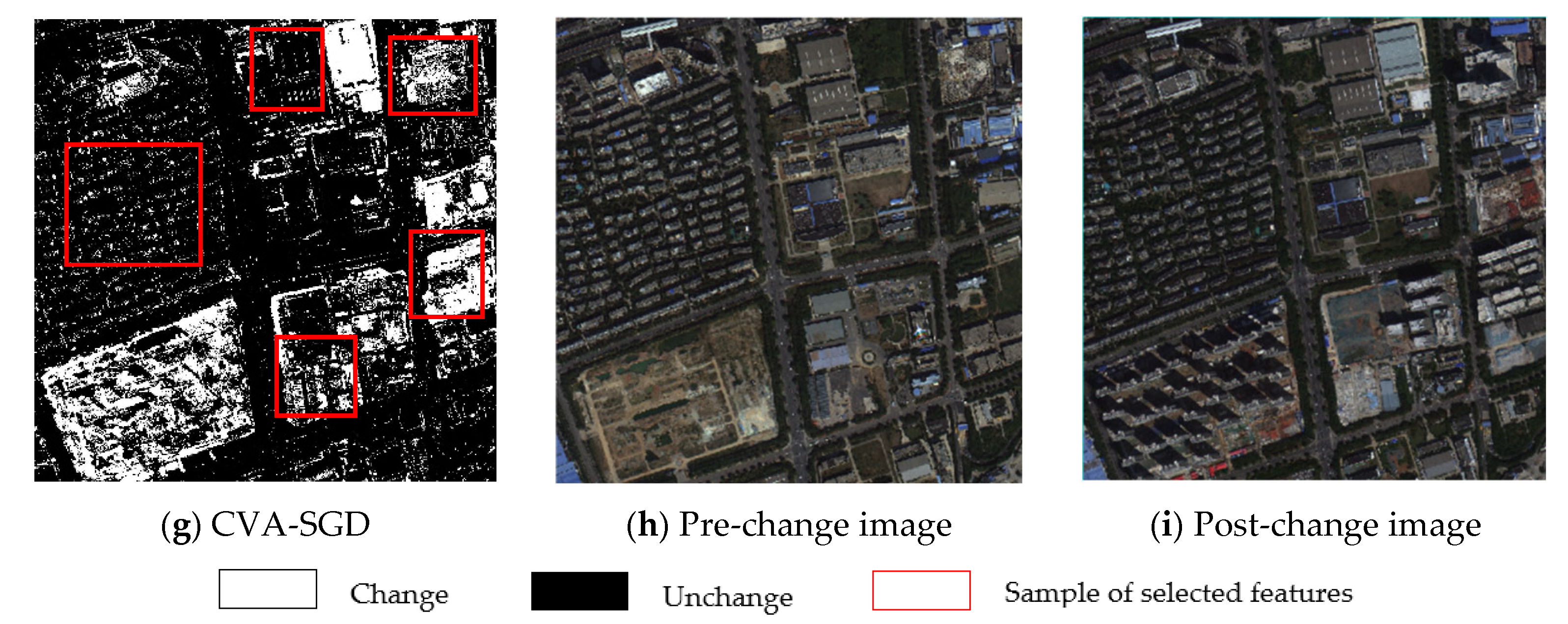
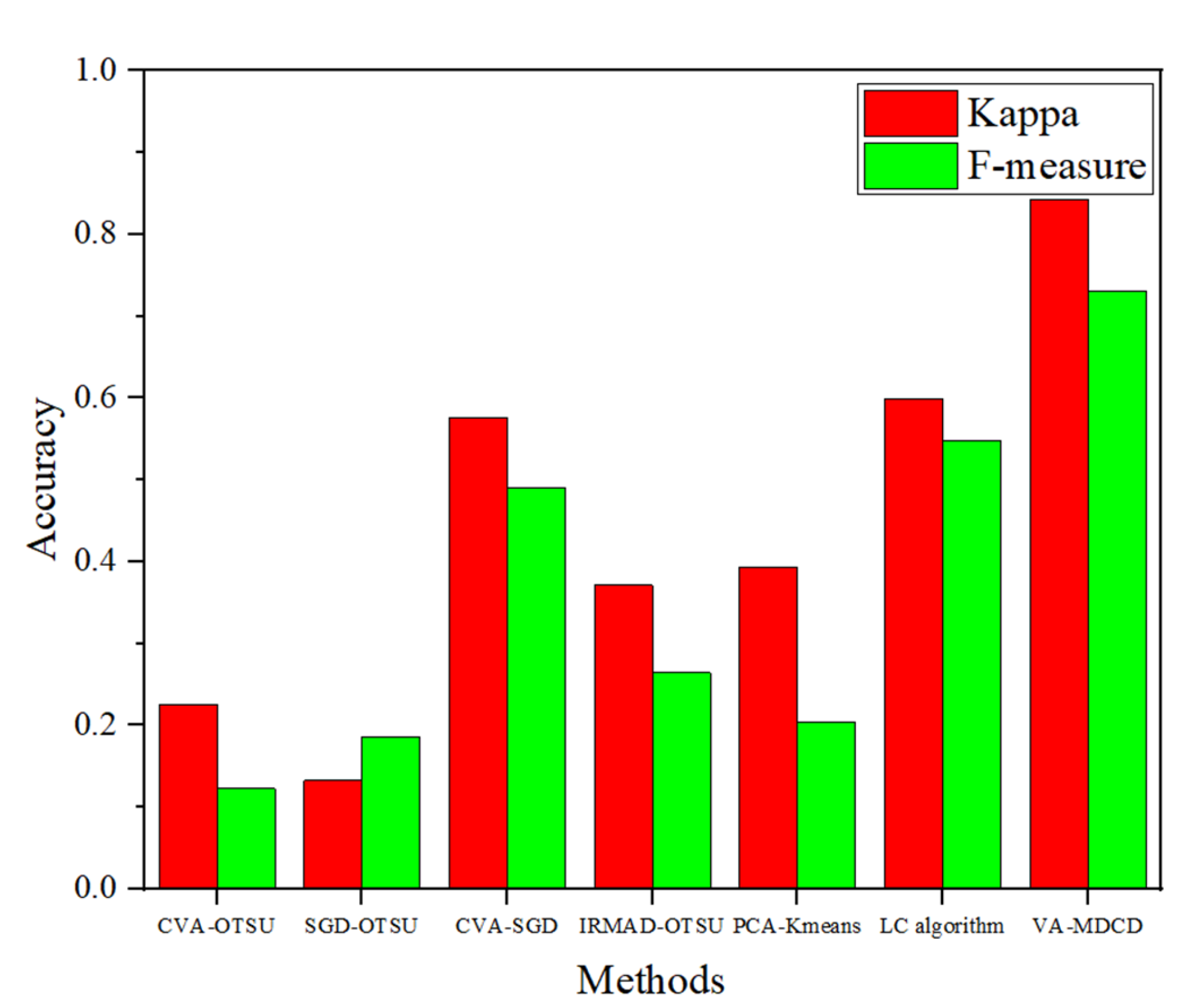
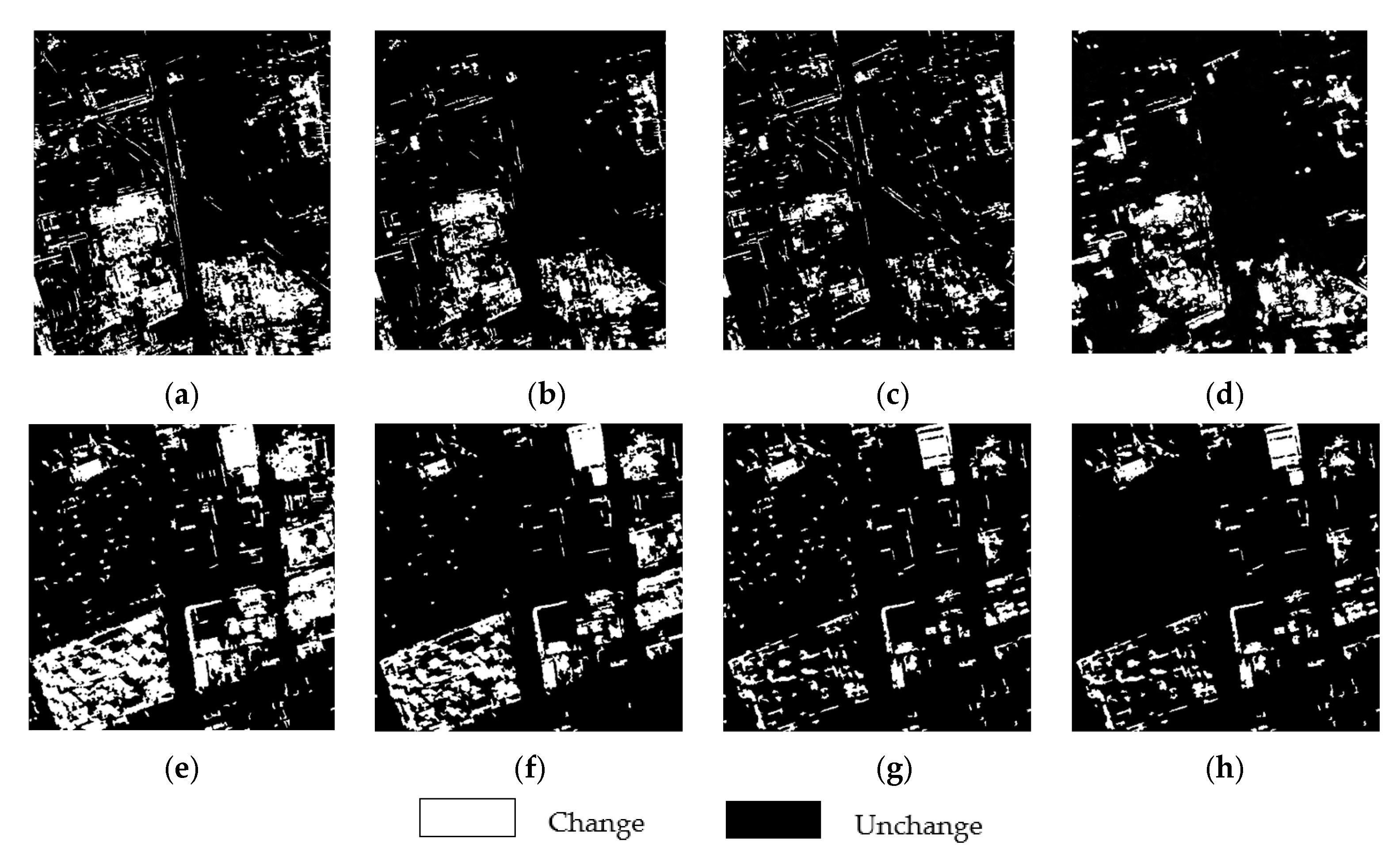
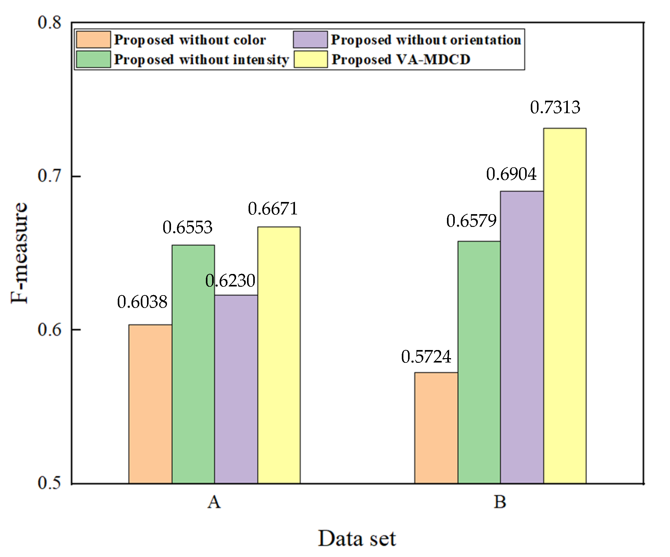
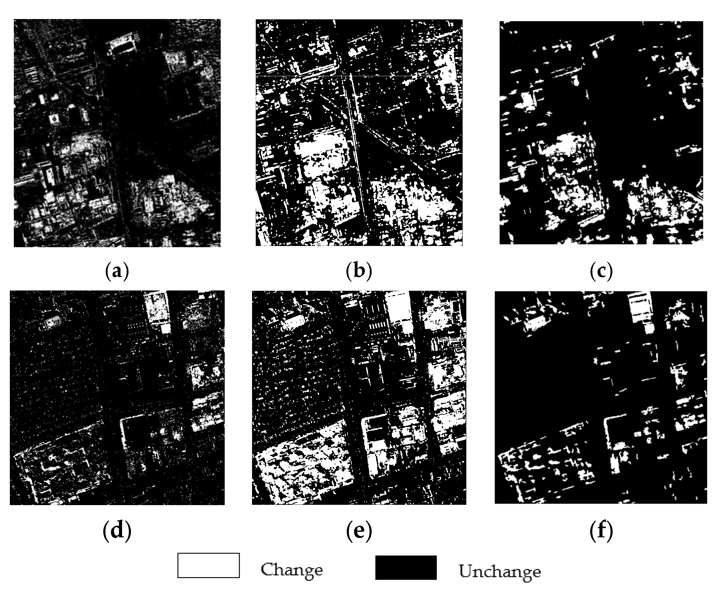
The experimental results obtained from two sets of VHR images validate the efficacy of the proposed VA-MDCD. First, our proposed VA-MDCD method can be used on VHR images and it can effectively identify the changes in VHR images. The experimental results show that this method not only has a higher F-measure and Kappa compared with other methods, but it can also reduce the FA of CVA-SGD. Second, the addition of a visual attention model helps to utilize the overall information of VHR images. Compared with the method using only spectral features, the proposed method can be applied to a wide range of VHR images. It not only contains the spectral information of the image, but also highlights the color, intensity and orientation information of the image. Third, after a statistical analysis of multiple pairs of samples that are easily affected by shooting angles, we conclude that the proposed VA-MDCD can reduce the error caused by the direct fusion of multiple difference images. In addition, we also designed an ablation experiment, and the model included four structures. Four groups of experiments were conducted on two datasets, respectively, and the F-measure value was calculated. The experimental results show that the proposed method has a higher F-measure, and the change detection effect of VA-MDCD proposed in this paper is better for both dataset compared to not using a color module, intensity module or orientation module.

The method in this paper is based on an improvement of unsupervised algorithms. Due to the lack of training samples, the method does not perform well when applied to extremely complex scenes. Therefore, in future studies, we will consider combining a visual attention model with deep learning and taking the visual attention model as the method of sample generation. This will not only reduce the complexity of manual sample labeling, but also generate reliable training samples.

References

1. Shahat Osman, A.M.; Elragal, A. Smart cities and big data analytics: A data-driven decision-making use case. Smart Cities 2021, 4, 286–313. [Google Scholar]
2. Grübel, J.; Thrash, T.; Aguilar, L.; Gath-Morad, M.; Chatain, J.; Sumner, R.W.; Hölscher, C.; Schinazi, V.R. The Hitchhiker’s Guide to Fused Twins: A Review of Access to Digital Twins In Situ in Smart Cities. Remote Sens. 2022, 14, 3095. [Google Scholar]
3. Zhu, J.; Wu, P. Towards effective BIM/GIS data integration for smart city by integrating computer graphics technique. Remote Sens. 2021, 13, 1889. [Google Scholar] [CrossRef]
4. Long, H.; Zhang, Y.; Ma, L.; Tu, S. Land use transitions: Progress, challenges and prospects. Land 2021, 10, 903. [Google Scholar]
5. Winkler, K.; Fuchs, R.; Rounsevell, M.; Herold, M. Global land use changes are four times greater than previously estimated. Nat. Commun. 2021, 12, 2501. [Google Scholar] [PubMed]
6. Asokan, A.; Anitha, J. Change detection techniques for remote sensing applications: A survey. Earth Sci. Inform. 2019, 12, 143–160. [Google Scholar]
7. Chughtai, A.H.; Abbasi, H.; Karas, I.R. A review on change detection method and accuracy assessment for land use land cover. Remote Sens. Appl. Soc. Environ. 2021, 22, 100482. [Google Scholar]
8. Du, P.; Liu, S.; Xia, J.; Zhao, Y. Information fusion techniques for change detection from multi-temporal remote sensing images. Inf. Fusion 2013, 14, 19–27. [Google Scholar]
9. Zhang, C.; Yue, P.; Tapete, D.; Jiang, L.; Shangguan, B.; Huang, L.; Liu, G. A deeply supervised image fusion network for change detection in high resolution bi-temporal remote sensing images. ISPRS J. Photogramm. Remote Sens. 2020, 166, 183–200. [Google Scholar]
10. Liu, Y.; Liu, J.; Ning, X.; Li, J. MS-CNN: Multiscale recognition of building rooftops from high spatial resolution remote sensing imagery. Int. J. Remote Sens. 2022, 43, 270–298. [Google Scholar]
11. Xin, J.; Zhang, X.; Zhang, Z.; Fang, W. Road extraction of high-resolution remote sensing images derived from DenseUNet. Remote Sens. 2019, 11, 2499. [Google Scholar]
12. Chen, F.; Qin, F.; Peng, G.; Chen, S. Fusion of remote sensing images using improved ICA mergers based on wavelet decomposition. Procedia Eng. 2012, 29, 2938–2943. [Google Scholar]
13. Gong, J.; Sui, H.; Sun, K.; Ma, G.; Liu, J. Object-level change detection based on full-scale image segmentation and its application to Wenchuan Earthquake. Sci. China Ser. E Technol. Sci. 2008, 51, 110–122. [Google Scholar]
14. Linke, J.; McDermid, G.; Laskin, D.; McLane, A.; Pape, A.; Cranston, J.; Hall-Beyer, M.; Franklin, S. A disturbance-inventory framework for flexible and reliable landscape monitoring. Photogramm. Eng. Remote Sens. 2009, 75, 981–995. [Google Scholar] [CrossRef]
15. Blaschke, T. Towards a framework for change detection based on image objects. Göttinger Geogr. Abh. 2005, 113, 1–9. [Google Scholar]
16. Ab Wahab, M.N.; Nazir, A.; Ren, A.T.Z.; Noor, M.H.M.; Akbar, M.F.; Mohamed, A.S.A. Efficientnet-lite and hybrid CNN-KNN implementation for facial expression recognition on raspberry pi. IEEE Access 2021, 9, 134065–134080. [Google Scholar] [CrossRef]
17. Pires de Lima, R.; Marfurt, K. Convolutional neural network for remote-sensing scene classification: Transfer learning analysis. Remote Sens. 2019, 12, 86. [Google Scholar]
18. Khelifi, L.; Mignotte, M. Deep learning for change detection in remote sensing images: Comprehensive review and meta-analysis. IEEE Access 2020, 8, 126385–126400. [Google Scholar]
19. Coppin, P.; Jonckheere, I.; Nackaerts, K.; Muys, B.; Lambin, E. Review ArticleDigital change detection methods in ecosystem monitoring: A review. Int. J. Remote Sens. 2004, 25, 1565–1596. [Google Scholar] [CrossRef]
20. Celik, T. Change detection in satellite images using a genetic algorithm approach. IEEE Geosci. Remote Sens. Lett. 2010, 7, 386–390. [Google Scholar] [CrossRef]
21. Bruzzone, L.; Prieto, D.F. Automatic analysis of the difference image for unsupervised change detection. IEEE Trans. Geosci. Remote Sens. 2000, 38, 1171–1182. [Google Scholar] [CrossRef] [Green Version]
22. Lu, D.; Li, G.; Moran, E. Current situation and needs of change detection techniques. Int. J. Image Data Fusion 2014, 5, 13–38. [Google Scholar] [CrossRef]
23. Sumaiya, M.; Kumari, R.S.S. Logarithmic mean-based thresholding for SAR image change detection. IEEE Geosci. Remote Sens. Lett. 2016, 13, 1726–1728. [Google Scholar] [CrossRef]
24. Sun, Y.; Lei, L.; Guan, D.; Kuang, G. Iterative robust graph for unsupervised change detection of heterogeneous remote sensing images. IEEE Trans. Image Process. 2021, 30, 6277–6291. [Google Scholar] [CrossRef] [PubMed]
25. Chen, J.; Lu, M.; Chen, X.; Chen, J.; Chen, L. A spectral gradient difference based approach for land cover change detection. ISPRS J. Photogramm. Remote Sens. 2013, 85, 1–12. [Google Scholar] [CrossRef]
26. Yan, Z.; Huazhong, R.; Desheng, C. The research of building earthquake damage object-oriented change detection based on ensemble classifier with remote sensing image. In Proceedings of the IGARSS 2018-2018 IEEE International Geoscience and Remote Sensing Symposium, Valencia, Spain, 22–27 July 2018; pp. 4950–4953. [Google Scholar]
27. Malila, W.A. Change vector analysis: An approach for detecting forest changes with Landsat. In Proceedings of the LARS Symposia, West Lafayette, IN, USA, 3–6 June 1980; 385p. [Google Scholar]
28. Xing, H.; Hou, D.; Lu, M.; Chen, J. A Land Cover Change Detection Method Based On Change Difference Map Fusion. ISPRS Ann. Photogramm. Remote Sens. Spat. Inf. Sci. 2019, IV-2/W5, 239–243. [Google Scholar] [CrossRef] [Green Version]
29. Hearst, M.A.; Dumais, S.T.; Osuna, E.; Platt, J.; Scholkopf, B. Support vector machines. IEEE Intell. Syst. Their Appl. 1998, 13, 18–28. [Google Scholar] [CrossRef] [Green Version]
30. Breiman, L. Random forests. Mach. Learn. 2001, 45, 5–32. [Google Scholar] [CrossRef] [Green Version]
31. Huang, G.-B.; Zhu, Q.-Y.; Siew, C.-K. Extreme learning machine: Theory and applications. Neurocomputing 2006, 70, 489–501. [Google Scholar]
32. Hou, X.; Zhang, L. Saliency detection: A spectral residual approach. In Proceedings of the 2007 IEEE Conference on Computer vision and Pattern Recognition, Minneapolis, MN, USA, 17–22 June 2007; pp. 1–8. [Google Scholar]
33. Goferman, S.; Zelnik-Manor, L.; Tal, A. Context-aware saliency detection. IEEE Trans. Pattern Anal. Mach. Intell. 2011, 34, 1915–1926. [Google Scholar] [CrossRef] [PubMed] [Green Version]
34. Liu, Y.; Cheng, M.-M.; Hu, X.; Wang, K.; Bai, X. Richer convolutional features for edge detection. In Proceedings of the IEEE Conference on Computer Vision and Pattern Recognition, Honolulu, HI, USA, 21–26 July 2017; pp. 3000–3009. [Google Scholar]
35. Ronneberger, O.; Fischer, P.; Brox, T. U-net: Convolutional networks for biomedical image segmentation. In Proceedings of the Medical Image Computing and Computer-Assisted Intervention–MICCAI 2015: 18th International Conference, Munich, Germany, 5–9 October 2015; Proceedings, Part III 18. Springer: Berlin/Heidelberg, Germany, 2015; pp. 234–241. [Google Scholar]
36. Zhong, Z.; Jin, L.; Xie, Z. High performance offline handwritten chinese character recognition using googlenet and directional feature maps. In Proceedings of the 2015 13th International Conference on Document Analysis and Recognition (ICDAR), Tunis, Tunisia, 23–26 August 2015; pp. 846–850. [Google Scholar]
37. Szegedy, C.; Ioffe, S.; Vanhoucke, V.; Alemi, A. Inception-v4, inception-resnet and the impact of residual connections on learning. In Proceedings of the AAAI Conference on Artificial Intelligence, San Francisco, CA, USA, 4–9 February 2017. [Google Scholar]
38. Nemoto, K.; Hamaguchi, R.; Sato, M.; Fujita, A.; Imaizumi, T.; Hikosaka, S. Building change detection via a combination of CNNs using only RGB aerial imageries. In Proceedings of the Remote Sensing Technologies and Applications in Urban Environments II, Warsaw, Poland, 11–12 September 2017; pp. 107–118. [Google Scholar]
39. Pomente, A.; Picchiani, M.; Del Frate, F. Sentinel-2 change detection based on deep features. In Proceedings of the IGARSS 2018-2018 IEEE International Geoscience and Remote Sensing Symposium, Valencia, Spain, 22–27 July 2018; pp. 6859–6862. [Google Scholar]
40. Lei, T.; Xue, D.; Ning, H.; Yang, S.; Lv, Z.; Nandi, A.K. Local and global feature learning with kernel scale-adaptive attention network for VHR remote sensing change detection. IEEE J. Sel. Top. Appl. Earth Obs. Remote Sens. 2022, 15, 7308–7322. [Google Scholar]
41. Wu, C.; Chen, H.; Du, B.; Zhang, L. Unsupervised change detection in multitemporal VHR images based on deep kernel PCA convolutional mapping network. IEEE Trans. Cybern. 2021, 52, 12084–12098. [Google Scholar] [CrossRef]
42. He, D.; Zhang, Y.; Song, H. A novel saliency map extraction method based on improved Itti’s model. In Proceedings of the 2010 International Conference on Computer and Communication Technologies in Agriculture Engineering, Chengdu, China, 12–13 June 2010; pp. 323–327. [Google Scholar]
43. Tang, Z.; Zhang, H.; Pun, C.M.; Yu, M.; Yu, C.; Zhang, X. Robust image hashing with visual attention model and invariant moments. IET Image Process. 2020, 14, 901–908. [Google Scholar]
44. Tang, T.; Hu, P.; Wu, G. Influence of promotion mode on purchase decision based on multilevel psychological distance dimension of visual attention model and data mining. Concurr. Comput. Pr. Exp. 2021, 33, e5587. [Google Scholar]
45. Li, H.; Manjunath, B.; Mitra, S.K. Multisensor image fusion using the wavelet transform. Graph. Models Image Process. 1995, 57, 235–245. [Google Scholar] [CrossRef]
46. Otsu, N. A threshold selection method from gray-level histograms. IEEE Trans. Syst. Man Cybern. 1979, 9, 62–66. [Google Scholar] [CrossRef] [Green Version]
47. Jia, Y.; Hao, C.; Wang, K. A new saliency object extraction algorithm based on Itti’s model and region growing. In Proceedings of the 2019 IEEE International Conference on Mechatronics and Automation (ICMA), Tianjin, China, 4–7 August 2019; pp. 224–228. [Google Scholar]
48. Tang, L.; Li, H.; Chen, T. Extract salient objects from natural images. In Proceedings of the 2010 International Symposium on Intelligent Signal Processing and Communication Systems, Chengdu, China, 6–8 December 2010; pp. 1–4. [Google Scholar]
49. Yan, Q.; Xu, L.; Shi, J.; Jia, J. Hierarchical saliency detection. In Proceedings of the IEEE Conference on Computer Vision and Pattern Recognition, Portland, OR, USA, 23–28 June 2013; pp. 1155–1162. [Google Scholar]
50. Liu, N.; Cao, Z.; Cui, Z.; Pi, Y.; Dang, S. Multi-layer abstraction saliency for airport detection in SAR images. IEEE Trans. Geosci. Remote Sens. 2019, 57, 9820–9831. [Google Scholar]
51. Amolins, K.; Zhang, Y.; Dare, P. Wavelet based image fusion techniques—An introduction, review and comparison. ISPRS J. Photogramm. Remote Sens. 2007, 62, 249–263. [Google Scholar] [CrossRef]
52. Nackaerts, K.; Vaesen, K.; Muys, B.; Coppin, P. Comparative performance of a modified change vector analysis in forest change detection. Int. J. Remote Sens. 2005, 26, 839–852. [Google Scholar] [CrossRef]
53. Adelson, E.H.; Anderson, C.H.; Bergen, J.R.; Burt, P.J.; Ogden, J.M. Pyramid methods in image processing. RCA Eng. 1984, 29, 33–41. [Google Scholar]
54. Lan, Z.; Lin, M.; Li, X.; Hauptmann, A.G.; Raj, B. Beyond gaussian pyramid: Multi-skip feature stacking for action recognition. In Proceedings of the IEEE Conference on Computer Vision and Pattern Recognition, Boston, MA, USA, 7–12 June 2015; pp. 204–212. [Google Scholar]
55. Ding, L.; Goshtasby, A. On the Canny edge detector. Pattern Recognit. 2001, 34, 721–725. [Google Scholar] [CrossRef]
56. Rong, W.; Li, Z.; Zhang, W.; Sun, L. An improved CANNY edge detection algorithm. In Proceedings of the 2014 IEEE International Conference on Mechatronics and Automation, Tianjin, China, 3–6 August 2014; pp. 577–582. [Google Scholar]
57. Xiao, A.; Wang, Z.; Wang, L.; Ren, Y. Super-resolution for “Jilin-1” satellite video imagery via a convolutional network. Sensors 2018, 18, 1194. [Google Scholar] [CrossRef] [PubMed] [Green Version]
58. Fan, Y.; Lou, D.; Zhang, C.; Wei, Y.; Jia, F. Information extraction technologies of iron mine tailings based on object-oriented classification: A case study of Beijing-2 remote sensing images of the Qianxi Area, Hebei Province. Remote Sens. Nat. Resour. 2021, 33, 153–161. [Google Scholar]
59. Hoffmann, W. Iterative algorithms for Gram-Schmidt orthogonalization. Computing 1989, 41, 335–348. [Google Scholar] [CrossRef]
60. Falco, N.; Marpu, P.R.; Benediktsson, J.A. Comparison of ITPCA and IRMAD for automatic change detection using initial change mask. In Proceedings of the 2012 IEEE International Geoscience and Remote Sensing Symposium, Munich, Germany, 22–27 July 2012; pp. 6769–6772. [Google Scholar]
61. Li, H.-C.; Longbotham, N.; Emery, W.J. Unsupervised change detection of remote sensing images based on semi-nonnegative matrix factorization. In Proceedings of the 2014 IEEE Geoscience and Remote Sensing Symposium, Quebec City, QC, Canada, 13–18 July 2014; pp. 1289–1292. [Google Scholar]
62. Stehman, S. Estimating the kappa coefficient and its variance under stratified random sampling. Photogramm. Eng. Remote Sens. 1996, 62, 401–407. [Google Scholar]
63. Wang, J.; Liu, J.; Zhang, Y.; Zhu, H.; Han, Y.; Zhang, Y.; Zhou, R.; Hong, Z.; Yang, S. An Image Strategy Based on Saliency Detection Using Luminance Contrast for Artificial Vision with Retinal Prosthesis. In Proceedings of the Sixth International Congress on Information and Communication Technology: ICICT 2021, London, UK, 25–26 February 2021; Springer: Berlin/Heidelberg, Germany, 2022; Volume 3, pp. 273–281. [Google Scholar]
64. Singh, S.K.; Srivastava, R. A novel probabilistic contrast-based complex salient object detection. J. Math. Imaging Vis. 2019, 61, 990–1006. [Google Scholar] [CrossRef]
65. Zhu, M.; Jiao, L.; Liu, F.; Yang, S.; Wang, J. Residual spectral–spatial attention network for hyperspectral image classification. IEEE Trans. Geosci. Remote Sens. 2020, 59, 449–462. [Google Scholar]
Figure 1. The flow chart of the proposed VA-MDCD.
Remotesensing 15 03799 g001
Figure 2. Change vector analysis.
Remotesensing 15 03799 g002
Figure 3. Model structure.
Remotesensing 15 03799 g003
Figure 4. The procedure of LC algorithm.
Remotesensing 15 03799 g004
Figure 5. The procedure of wavelet transform fusion.
Remotesensing 15 03799 g005
Figure 6. JL-1 remote sensing images (a) in 2018; (b) in 2019. (c) Ground truth image.
Remotesensing 15 03799 g006
Figure 7. The selected ground object samples.
Remotesensing 15 03799 g007aRemotesensing 15 03799 g007b
Figure 8. Change magnitude images on the JL-1 dataset.
Remotesensing 15 03799 g008
Figure 9. Change detection results. (a) CVA-OTSU; (b) SGD-OTSU; (c) IRMAD-OTSU; (d) PCA kmeans; (e) LC algorithm; (f) VA-MDCD; (g) CVA-SGD; (h) pre-change image; (i) post-change image.
Remotesensing 15 03799 g009
Figure 10. Kappa and F-measure coefficients of different change detection methods.
Remotesensing 15 03799 g010
Figure 11. BJ-2 remote sensing images (a) in 2018; (b) in 2021. (c) Ground truth.
Remotesensing 15 03799 g011
Figure 12. The selected ground object samples.
Remotesensing 15 03799 g012
Figure 13. Change magnitude images on BJ-2 dataset.
Remotesensing 15 03799 g013
Figure 14. Change detection results. (a) CVA-OTSU; (b) SGD-OTSU; (c) IRMAD-OTSU; (d) PCA kmeans; (e) LC algorithm; (f) VA-MDCD; (g) CVA-SGD; (h) pre-change image; (i) post-change image.
Remotesensing 15 03799 g014aRemotesensing 15 03799 g014b
Figure 15. Kappa and F-measure coefficients of different change detection methods.
Remotesensing 15 03799 g015
Figure 16. The change detection results of different model structures. (ad) are the four results of dataset A, namely the model without a color module, the model without an intensity module, the model without an orientation module and the proposed VA-MDCD method; (eh) are the four results of dataset B, namely the model without a color module, the model without an intensity module, the model without an orientation module and the proposed VA-MDCD method.
Remotesensing 15 03799 g016
Figure 17. The F-measure value of model change detection for different structures used in ablation experiments.
Remotesensing 15 03799 g017
Figure 18. Change detection results based on different visual saliency models. (a,d) are the change detection results of the LC algorithm for datasets A and B, respectively; (b,e) are the change detection results of the SR algorithm for datasets A and B, respectively; (c,f) are the change detection results of the VA-MDCD method for datasets A and B, respectively.
Remotesensing 15 03799 g018