Finding Misclassified Natura 2000 Habitats by Applying Outlier Detection to Sentinel-1 and Sentinel-2 Data

Abstract

The monitoring of Natura 2000 habitats (Habitat Directive 92/43/EEC) is a key activity ensuring the sufficient protection of European biodiversity. Reporting on the status of Natura 2000 habitats is required every 6 years. Although field mapping is still an indispensable source of data on the status of Natura 2000 habitats, and very good field-based data exist in some countries, keeping the field-based habitat maps up to date can be an issue. Remote sensing techniques represent an excellent alternative. Here, we present a new method for detecting habitats that were likely misclassified during the field mapping or that have changed since then. The method identifies the possible habitat mapping errors as the so-called “attribute outliers”, i.e., outlying observations in the feature space of all relevant (spectral and other) characteristics of an individual habitat patch. We used the Czech Natura 2000 Habitat Layer as field-based habitat data. To prepare the feature space of habitat characteristics, we used a fusion of Sentinel-1 and Sentinel-2 satellite data along with a Digital Elevation Model. We compared outlier ratings using the robust Mahalanobis distance and Local Outlier Factor using three different thresholds (Tukey rule, histogram-based Scott’s rule, and 95% quantiles in χ² distribution). The Mahalanobis distance thresholded by the 95% χ² quantile achieved the best results, and, because of its high specificity, appeared as a promising tool for identifying erroneously mapped or changed habitats. The presented method can, therefore, be used as a guide to target field updates of Natura 2000 habitat maps or for other habitat/land cover mapping activities where the detection of misclassifications or changes is needed.

1. Introduction

Natura 2000 is a Europe-wide network of protected areas established to protect endangered species and natural and near-natural habitats. The conservation and monitoring of Natura 2000 sites is defined in the European Habitat Directive 92/43/EEC, which states that the conservation status of Natura 2000 sites and habitats must be reported every six years. Because whole-country field investigations are time-consuming and costly [1], satellite imagery has emerged as a promising technology for the monitoring of Natura 2000 sites [2]. A suitable remote sensing method can significantly reduce the costs of Natura 2000 sites monitoring and improve public control over environmental protection [3,4].

So far, many studies have demonstrated the potential of satellite data for general monitoring of Natura 2000 sites or directly for detecting and mapping individual Natura 2000 habitats [5,6,7]. Studies based on the classification of multispectral (e.g., Rapid Eye, Sentinel-2) data [1,8], hyperspectral data [9,10,11], or fusion of multispectral and radar data (e.g., fusion of Sentinel-2 and Sentinel-1 [12,13]) achieve promising precision in the identification of individual habitats and encouraging results. However, the studies mostly focus on just a few habitats at the regional level; where a higher number of habitats were classified, the studies were only at a local level. The lack of studies dealing with the classification of a wide range of habitat types within large areas (e. g., whole countries) suggests that the remote-sensing-based classification of all habitats at the national level remains challenging and that field habitat mapping is still valuable for the monitoring of Natura 2000 habitats.

Although field mapping is still an indispensable source of data on the status of habitats and very good field-based data exist in some countries, keeping them up to date without employing remote sensing techniques can be an issue. The Czech Republic is one such example, where detailed (cartographic ratio of 1:10,000) field mapping of all Natura 2000 habitats nationwide was carried out in 2001–2014 [14], based on which a Habitat Layer of the Czech Republic was subsequently created [15,16]. This created a comprehensive data source not only for nature conservation and biodiversity research but also for various sectors of the state administration [14,17,18]. The habitat layer is now being updated, again using field mapping, but ways to simplify and speed up the update using remote sensing are being explored. For example, finding a method capable of identifying habitat segments that were likely misclassified in the original mapping or have changed since the last mapping could make the process more effective, directing field research toward such habitats. Hence, as in some other EU countries, the main challenge remains to keep such field-based data up to date, to clean possible mapping errors (i.e., misidentified habitat classes), and to reveal ongoing gradual or sudden habitat changes as automatically as possible with the least possible expenditure.

Change detection (CD) is a common remote sensing method used to reveal changes in the reflectance characteristics of the mapped surfaces, and many different CD methods have been developed over time (an overview can be found in reference [19]). The CD analysis could be challenging and affected by the detection of unwanted changes such as phenological stages, sudden climatic events (snow, hail, drought, etc.), or differences in observation geometry. It could also be susceptible to errors caused by atmospheric correction or differences in the used sensors [20]. Here, we are introducing a method based on the outlierness of a particular observation in the space of its spectral and other characteristics. The benefit of the proposed method lies in its capability to perform change detection under multi-temporal observation or even using observation from a single time point when comparing the data with existing classification. The robustness of the method consists in using the single-temporal change detection, where effects of climatic events, geometry, atmosphere, or sensors is minimized. The main idea of the method is that changed or misclassified classes should be identifiable as those differing from the correctly classified habitats. Therefore, we identified the possible habitat mapping errors or changes as the so-called “attribute outliers”, i.e., outlying observations in the feature space of all relevant (spectral and other) segment characteristics.

Using Sentinel-1 and Sentinel-2 data, this study aimed to develop a repeatable method for the identification of habitats that were potentially misidentified during field mapping or have changed since the mapping. In practical terms, such a method would help to target field efforts for mapping updates to such places.

2. Materials and Methods

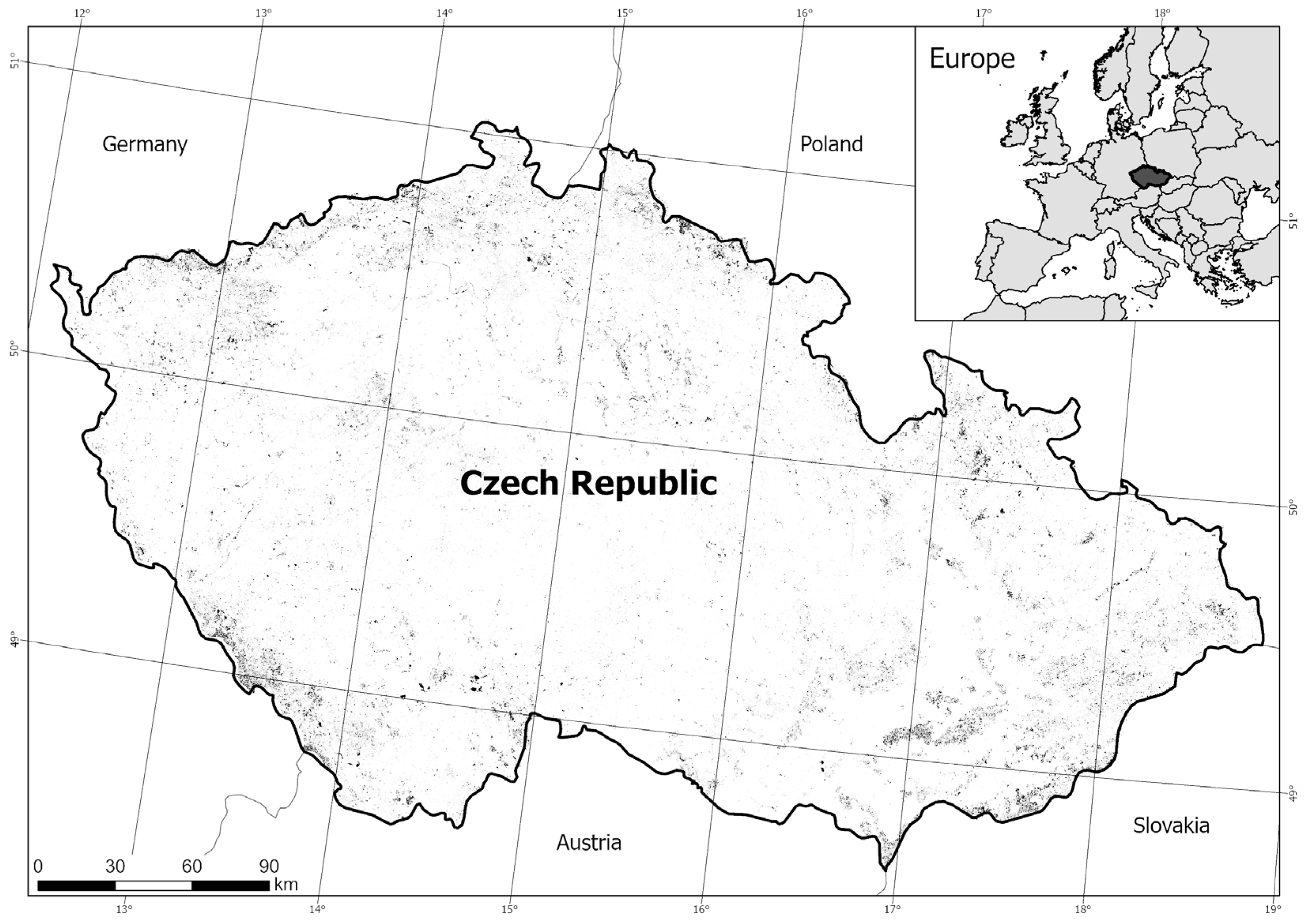
2.1. Study Area and Field-Based Habitat Data

We used the Habitat Layer of the Czech Republic (hereinafter Habitat Layer) covering the whole country for our research (see Figure 1). The Habitat Layer was originally created to delineate Special Areas of Conservation (SACs) under the Habitat Directive and its first version was completed in 2005. Since 2006, it has been systematically updated by field mapping led by Nature Conservation Agency, with one-twelfth of the Czech Republic mapped each year. The layer is available under a free open license from the Nature Conservation Agency (https://data.nature.cz, accessed on 5 December 2022).

To find potentially misclassified or substantially changed habitat segments, we used the basic division of the Habitat Catalogue [21], which is compatible with habitat types delimited in Annex I of the Habitats Directive. Hence, the list of Natura 2000 habitats used in our study was as follows: Water (Streams and water bodies); Wetlands (Wetlands and riverine vegetation); Mires (Springs and mires); Screes (Cliffs and boulder screes); Alpines (Alpine treeless habitats); Grass (Secondary grassland and heathland); Scrubs (Scrubs); and Forests (Woodland). A detailed description of the habitats is available in reference [21].

2.2. Satellite and DEM Data

We used Sentinel and Digital Elevation Model (DEM) data to find patches (segments) where habitats were potentially misidentified during mapping or have changed since mapping. The Sentinel satellites are operated by the European Commission, which provides the data free of charge. The Sentinel-2 satellite, with its 13 optical bands, is ideal for identifying the species composition of vegetation [22,23,24]. Despite the many advantages of Sentinel-2 satellites, the applicability in the Czech Republic is limited by cloud cover (Central Bohemia was completely cloud-free only during six satellite flybys in 2018 and only once in 2022). For this reason, we created one representative seamless and cloud-free mosaic of the Czech Republic within the growing season of the years 2018 and 2022 (details in Section 2.3).

To overcome the disadvantages of Sentinel-2 and deliver information about the temporal dynamics of Natura 2000 habitats during the growing season of the year under study, we used Sentinel-1 microwave observation because of its all-weather, day-to-night observation capacity. Since Sentinel-1 has its own illumination source, it allows you to have complete control over the polarization of the transmitted and received signal. Sentinel-1 measures in two polarizations: co-polarization VV (vertical emitting, vertical receiving) and cross-polarization VH (vertical emitting, horizontal receiving). While the source of the VV signal is direct reflections from the earth’s surface, or double reflections from mutually perpendicular objects (predominant in cities), the primary source of the VH signal is the so-called volume scattering, in which the signal enters the object and is subsequently reflected many times and interacts with each other. The result is a depolarization of the emitted V-polarized signal and an increase in the received H-polarized signal. The main source of volume scattering (represented by VH polarization) is vegetation. As shown in previous studies, VH polarization could respond well to the vegetation status [25,26,27,28,29] and, therefore, it was used in this study.

The digital elevation model EU DEM version 1.1 (https://land.copernicus.eu/imagery-in-situ/eu-dem/eu-dem-v1.1, accessed on 5 December 2022) was selected to calculate terrain characteristics. The elevation is defined here according to the European Vertical Reference System (EVRS). The spatial resolution is 25 m with an absolute error in elevation of ±7 m RMSE.

2.3. Spatial Data Processing

We used Habitat Layer segments (polygons) that were updated in the field in 2018 and 2022. We chose these two years both to fit the Sentinel-1 and -2 missions and to test the search for outliers on two samples (years) that are as far apart in time as possible. We worked only with natural and near-natural habitats, i.e., we excluded habitats strongly influenced or created by humans (category X according to the Czech Habitat Catalogue). We also excluded so-called mosaics, i.e., polygons consisting of several habitat types. To remove possible edge pixel problems, possible shadowing due to nearby obstacles or possible misregistration of product [30]; we shrunk the remaining polygons by 20 m, which is a spatial resolution in bands essential for vegetation identification of Sentinel-2. The registration of habitat polygons to satellite data was examined visually and no significant shift was observed. Subsequently, all the polygons smaller than the size of one pixel (i.e., 400 m²) were removed from the analysis. After this, 233,966 polygons remained for the outliers analysis.

We used the Sentinel-2 Global Mosaic service (https://apps.sentinel-hub.com/mosaic-hub/, accessed on 5 December 2022) to create a seamless mosaic over the whole Czech Republic covering the growing season (March-October) in the years 2018 and 2022. The resulting mosaic is formed from medoids of the pixels of each image cleared from clouds, cloud shadows, snow-covered areas, and areas significantly affected by the atmosphere. The medoid is a pixel with the smallest differences from other pixels at the same location but at different times. In this way, the most representative pixel at a given location was always selected [31]. Bands 1, 9, and 10 were omitted because their purpose is atmosphere description and, therefore, they have minimal added value for ground observation; moreover, they have a coarse resolution of 60 m per pixel, which does not correspond to the minimal polygon size. The final band selection is in

Table 1. Characteristic of Sentinel-2 Bands used for the final product.

Band Number	2	3	4	5	6	7	8	8a	11	12
Band name	Blue	Green	Red	Red Edge	Red Edge	Red Edge	NIR	Red Edge	SWIR	SWIR
Center (nm)	490	560	665	705	740	783	842	865	1610	2190
Width (nm)	65	35	30	15	15	20	115	20	90	180
Spatial resolution (m)	10	10	10	20	20	20	10	20	20	20

.

The microwave Sentinel-1 images were processed using the ASF HyP3 tool. The images were radiometrically corrected to the gamma-nought level (γ0). The terrain influence was removed using the Copernicus DEM digital terrain model terrain flattening. Additionally, 10 × 2 multi-looking was performed to suppress noise and obtain square pixels. The whole computation was performed using the algorithms of the GAMMA software 5.1.1. More information is available at https://hyp3-docs.asf.alaska.edu/guides/rtc_product_guide/, accessed on 6 December 2022.

The individual images were subsequently used to create nationwide mosaics at a step of one month during the growing season (March–October) for the years 2018 and 2022. We used the Quick Mosaic tool in ENVI 5.6 for the mosaic generation.

We used the EU DEM to account for the effects of elevation, slope, and exposure on cardinal directions of the spectral characteristics of habitats during the growing season. We calculated the average elevation for each polygon of the Natura 2000 habitat, as well as the average slope and the prevailing direction to the cardinal points. This was carried out in ArcGIS Pro 2.7.0 [32], using the Slope and Aspect functions.

The mean, median, and standard deviations were calculated for each mentioned Sentinel-1 and Sentinel-2 band. At the same time, the average slope and elevation were calculated along with the predominant exposure to the cardinal directions and the total polygon size. In total, 55 aggregated values for each of the 233,966 polygons were calculated using QGIS 3.22 [33] multiband zonal statistics. The overview of all the resulting variables is given in Appendix A.

2.4. Spectral Outliers Detection

As the main idea of this study states, the erroneously mapped habitats, or habitats that changed after their mapping, should be identifiable as those that differ in their attribute values from the correctly identified habitats of the same type. Therefore, we identified the possible habitat mapping errors as the so-called “attribute outliers”, i.e., outlying observations in the feature space of all relevant (spectral and other) segment characteristics. To characterize individual segments, we used the variables extracted for each polygon as described in the previous parts (see Appendix A). These variables were standardized to unit variance and zero mean. Subsequently, the principal component analysis (PCA) was applied to reduce the dimensionality of the feature space and prevent a redundant use of the same information stored in multiple mutually correlated features. The PCA was applied to each habitat type separately to reflect its specific attribute characteristics. To reduce the dimensionality, we then used the first n principal components that explained together 95% of the variability of the original features. With our data, the mean (±SD) n was 18 (±2.3) (see the biplots of the first two components for each habitat type in Appendix B).

We applied two principally different approaches to identify outliers in the space of the first n principal components. The first approach assumes the compactness of the segment characteristics distribution, i.e., that observations representing correctly mapped habitats (of a given type) lie close together while outliers are observations lying far from the center of this distribution. We used the robust Mahalanobis distance (hereafter referred to as MAH), as implemented in the robust package for R [34]. Mahalanobis distance is the distance of an observation from the center of the distribution relative to the thickness of the covariance ellipsoid in the corresponding direction. The estimation of the covariance ellipsoid itself is sensitive to the presence of outliers, and so we estimated it robustly using the method of Minimum Covariance Determinant [35] implemented in the same package. The result is a robust MAH distance computed for each segment.

The Local Outlier Factor (LOF [36]), implemented in the bigutilsr package for R, was the second approach we applied [37]. It relaxes the compactness assumption and identifies outliers as observations lying in locally “empty” or “sparse” parts of the distribution. To put it simply, each observation is evaluated based on its distance from neighbors relative to the mutual distances among these neighbors. The result is a relative LOF value computed for each observation.

For both approaches, the resulting MAH or LOF value had to be thresholded to decide whether the observation was an outlier or not. Similarly to PCA, this thresholding was performed for each habitat type separately. We applied three different types of thresholds. (1) First, we used the well-known Tukey rule, i.e., an outlier was the observation with the MAH/LOF value higher than the third quartile of all values plus 1.5 times their interquartile range. We used the modified version of this rule implemented in the package bigutilsr, corrected for a possible skewness of the distribution and for multiple comparisons [38]. (2) The second type of threshold we used, implemented in the same package as function hist_out, was based on the identification of a gap in the histogram of MAH/LOF values. The algorithm iteratively searches for an empty class in the histogram that lies above the 80th percentile of the data. If such a gap is found, all observations above this gap are considered outliers and the process is repeated for all the remaining observations. This is iterated until no gap is found. In each iteration, the class breaks are generated using the robust version of Scott’s rule [39]. This histogram-based approach has the advantage of being adaptable to the actual distribution of the data. (3) The third type of threshold was applied only to the MAH method and was based on an assumption that the MAH values follow the χ² distribution with n degrees of freedom, and identifies outliers as the observations lying above the (1–0.05/N)th quantile, where n is the number of variables, and N is the number of observations. The division by N is the Bonferroni correction for multiple testing. Because LOF values cannot be expected to follow the χ² distribution, this approach is not applicable to this method.

The combination of the MAH/LOF methods with the three types of thresholds gave rise to five different methods of identification of outliers, namely MAHTukey, MAHhist, MAHχ², LOFTukey, and LOFhist. Apart from these, a combination of all these five methods designated as “Any” was evaluated, in which an observation is classified as an outlier if it was identified as such by any of the remaining five methods.

2.5. Method Validation

We validated our method in two different ways. First, we randomly selected 722 segments and checked their “true” habitat type by visual assessment of the corresponding orthophoto image from Google Earth Pro. Because the assumed prevalence of the truly erroneously mapped segments was very low, we could not apply purely random sampling, as this would probably result in a sample with no true mistakes. Instead, we applied stratified random sampling, trying to equally represent in the validation sample the outliers identified by the individual methods in the individual habitat types, and then added a comparable number of randomly selected inliers (i.e., non-outliers) in each habitat type. Because of the highly unequal prevalence of outliers and habitat types in the dataset, and because the corresponding orthophoto image was not available for some segments and years or the “true” habitat could not be visually identified, the resulting validation sample was not completely balanced (see

Table 2. Numbers of classification errors and outliers (identified by the “Any” method) in the validation sample for the years 2018 and 2022.

Habitat Type	Mapping Errors 2018		Mapping Errors 2022		Outliers (“Any”) 2018		Outliers (“Any”) 2022
	Number	%	Number	%	Number	%	Number	%
Alpines	15	26.79	15	26.79	28	50.00	25	44.64
Scrubs	57	61.29	56	60.22	30	32.26	40	43.01
Forests	41	23.03	70	39.55	78	43.82	104	58.43
Wetlands	67	72.04	69	74.19	47	50.54	54	58.06
Mires	33	68.75	33	68.75	26	54.17	29	60.42
Screes	23	58.97	23	58.97	15	38.46	17	43.59
Grass	32	27.59	41	35.65	68	58.62	65	56.03
Water	14	14.14	23	23.23	70	70.71	72	72.73
Total	282	39.06	15	26.79	331	45.84	406	56.23

). We then compared the truly erroneously mapped segments with the outliers identified using the individual methods using sensitivity, specificity, positive predictive value (PPV), and negative predictive value (NPV), corrected for the partial verification bias (i.e., bias caused by unequal prevalences of true mistakes in the original and validation samples) using the extended Begg and Greenes method [40]. We computed these metrics both for all habitat types together (with applying a correction for their unequal prevalences) and for each habitat type individually. We also computed the bootstrapped 95% confidence intervals for these metrics. We used the PVBcorrect package for R [41] for these computations.

Second, we investigated how sensitive the presented methods are to different levels of destruction of Natura 2000 polygons. A typical cause of habitat destruction is the expansion of human activity [42]. For this reason, we identified polygons of natural habitats that are mapped as artificial surfaces in the OpenStreetMap (OSM) database. To achieve this, we extracted polygons of all buildings, quarries, parking, parking multistore, service, bicycle parking, and all roads except bridleways, cycleways, foodways, paths, all grade tracks, and unclassified roads from the OSM database. Since the road network is drawn only as a line, we created the resulting polygons using a 3 m buffer, which is the standard lane size in the country. By subsequently overlaying the polygon layer of natural habitats and the polygon layer of artificial surfaces from OSM, we calculated the percentage destruction for each polygon. For subsequent analysis, we selected only polygons with an overlap greater than 20% and we manually inspected them using orthophoto images to verify if they were really damaged. A total of 59 polygons with verified damage were selected (see Appendix E). We then identified for each polygon whether or not it was marked as an outlier by the “Any” method, which was the method performing best in the previous validation. Finally, we divided the damaged segments into classes based on their percentage destruction and, for each class, we calculated the percentage of damaged segments that were identified as outliers.

3. Results

The results showed that most polygons were probably correctly mapped during the ground survey and all the proposed methods identified only a small fraction (0.06–9.41%) of the input segments as outliers. The total number of identified outliers, however, differed substantially between the methods (see Figure 2). The lowest number of outliers (140 to 290 outliers, i.e., 0.06 to 0.12% of all analyzed segments, respectively) was identified by the LOF methods. The MAHhist and MAHTukey methods identified about 17 times more outliers (from 2377 to 4881, i.e., 1.02 to 2.09%). The largest number of outliers was identified by the MAHχ² method, which identified 20,401 (8.72%) and 22,002 (9.40%) outliers in 2018 and 2022, respectively. The results of the “Any” method was, obviously, most influenced by this largest number of outliers identified by the MAHχ² method, and, therefore, the resulting number of outliers for ANY was almost identical to MAHχ² with an additional 8 and 9 outliers identified by one of the LOF methods in 2018 and 2022, respectively. Compared to the differences between methods, the differences between years were minor (see Figure 2). The numbers of outliers identified in the individual habitat types, however, exhibited much larger interannual variability, and also differed largely between the types, both in totals and percentages (see Appendix C).

The structure of the validation sample is described in Table 2. The total number of outliers in particular years was slightly higher than the number of true classification errors. The prevalence of outliers was about 50–55%, while the prevalence of classification errors was about 40–45%. The difference between the number of outliers and classification errors varied a bit more for individual habitat types but, for most of the types, these values were also notably similar (see Table 2).

The sensitivity of individual methods after correcting for the partial verification bias and the unequal prevalence of habitat types (see Figure 3) was very low, especially for the methods using the histogram or Tukey rule thresholds, where it was between 0.1 and 3.9%. The corresponding specificities were above 98%. Applying the χ²-quantile threshold to the MAH method led to considerably higher sensitivity (17.3 resp. 21.6% in 2018 resp. 2022), at the cost of slightly lower specificity (93.2 resp. 94.3% in 2018 resp. 2022). Unsurprisingly, the “Any” method performed similarly to the MAHχ² method. The PPVs were surprisingly similar between the methods (about 40 to 60%), with the values from 2022 being consistently higher than those from 2018. Similarly, the NPV values ranged between 60 to 80% for all methods, with the values from 2022 being lower than those from 2018.

The variability in accuracy metrics between the individual habitat types (based on the MAHχ² method) was considerably higher (Figure 4), with the variability between years remaining low. For water habitats, all 14 and 23 mapping errors in 2018 and 2022, respectively, (see Table 2) were correctly identified as outliers, which led to a sensitivity of 100%. (It was, however, associated with the impossibility of computing confidence intervals due to the perfect separation problem.) The obvious cost of this high sensitivity of water habitats was slightly lower specificity, as the method actually marked 70 and 72 segments in 2018 and 2022, respectively, as outliers (see Table 2). The specificity, however, still remained above 80%. The second-best performance was observed for alpine habitats, with a sensitivity of about 70% and specificity of about 85%, accompanied by a PPV about 50% and NPV about 90%. Sensitivities of about 30–40% were found for forest and grassland habitats, with high specificities (more than 96%), as well as relatively high PPV and NPV. Wetlands showed a sensitivity of about 20%, specificity above 90%, and the highest PPV value (above 80%, although with a cost of NPV being only about 40%). The remaining habitat types (scrubs, mires, and screes) showed very low sensitivity values (about 5–10%).

Next, we evaluated the performance of the “Any” method with respect to the different levels of habitat destruction (Figure 5). We have found that, with as little as 20% of the area destroyed, the method was able to detect 78% of such degraded polygons. The detection capability increased further with increasing habitat destruction until it stabilized at around 91% for habitats with at least 60% of their area being destroyed.

4. Discussion

Even though the study area was the whole Czech Republic, with very difficult-to-classify habitats, our results show that the proposed method is partially successful in identifying mapping errors. When all habitat types are analyzed together, the MAHχ² method (i.e., the one with the highest sensitivity) would be able to reveal about 20% of real mapping errors, while only about 6% of correctly mapped segments would be misidentified as potential mapping errors. When the method identifies a segment as a possible mapping error, there would be about a 40–50% probability that it is truly a mapping error. The probability that a segment identified by the method as correctly mapped is truly correctly mapped would be about 80%.

Our results also show (see Figure 5) that the proposed method is effective even when only part of the habitat has been altered. For this part of the analysis, we only considered cases where a habitat destruction due to construction occurred. Even in the case of 20% habitat destruction, the proposed method detected a change in 78% of cases. The method’s reliability further increased to a maximum of 92% when 60% or more of the habitat was destroyed. This finding has important practical implications, as in most of the observed changes, the habitat is not completely destroyed, but rather gradually or partially transformed.

The proposed method is very flexible and suitable for many different applications. For example, a similar approach [43] was used to solve the one-class classification problem, where the authors also exploited outlier search from the overall hyperspectral data and achieved high classification accuracy that outperformed many other classifications approaches such as one-class random forests or positive and unsupervised learning.

The method showed the best performance for water habitats, where it revealed all mapping errors as outliers. It also performed relatively well for alpines, forests, grasslands, and wetlands, but the performance for other types was rather poor. Except for water, the sensitivities were generally not very high (the maximum was about 70% for alpines). Given the high specificities, however, it does not generate too much of a false signal and so even the relatively small fraction of revealed erroneously mapped habitats might still be valuable. The differences in the method performance between the habitat types can be easily explained by their spectral characteristics [44].

As we can see in Appendix D, some categories had more and some less different spectral characteristics. The water habitats are well separable from other categories (separability was above 1.9 (i.e., good separability) compared to other categories, except for wetlands. This was further reflected in Figure 6, where it can be seen that, in the case of map error occurrences, the habitat will probably appear as a significant attribute outlier. On the other hand, it can be seen from Appendix D that the category scrubs is very poorly separable from the others, except for water and alpines. Therefore, a slight change in the scrubs habitat (e.g., forestation or conversion to grassland) will not be revealed as an attribute outlier and such a change is difficult to detect. Figure 6 also suggests that there is quite clear inter-annual spectral variation within individual Natura 2000 habitats. This could further complicate some of the classical methods for classifying remote sensing data.

The low spectral separability of the habitat classes in our study area seems to prevent any reliable classification, which apparently contradicts results of other studies suggesting a high success rate of direct classification of the Natura 2000 habitats from satellite data. Based on Sentinel-2 satellite imagery, Le Dez et al. [5] was able to classify a total of 39 selected habitat types in an alluvial test site in western France covering an area of 260 km². They chose the random forest method for classification and the resulting accuracy was up to 98% when using a total of 9 images across the study period. Three selected grassland types were classified in Marcinkowska-Ochtyra [6] with an accuracy of up to 88% on a 25 km2 test site. A 72% success rate was achieved for a total of 18 different Natura 2000 habitat types in a study by Rapinel [7] on a 20 km² test site on the island of Corsica. However, these studies were always carried out on a limited sample of Natura 2000 habitat types and in a limited area.

In contrast to the aforementioned studies, habitat classification could be challenging for remote sensing at a whole country level. One reason is that, over a large area, the same habitats may be in different phenological phases at the same time (i.e., spectrally distinct from each other) and, thus, the classification algorithms may fail to assign them to the same habitat category, even though variables affecting phenology (e.g., elevation and terrain configuration) are also used for the classification. In this study, we suppressed the phenology problem using a medoid mosaic (see Section 2.5). A visual inspection of the results shows that a medoid mosaic effectively suppresses differences in phenology due to altitude and abrupt short-term habitat changes (e.g., water bloom). The second reason is that Natura 2000 habitat categories based on phytocenology are not always following spectral classes detectable by remote sensing. This leads to the definition of classes which do not necessarily correspond well with the remote sensing clusters (such as peatlands overgrown with bushes, dry wetlands, a forest that was in the early stage of development after planting, very sparse grass cover looking like bare soil, or scree completely overgrown with forest, etc.). This could be seen in Appendix D, where almost no or very limited separability of classes occurs over Natura 2000 habitats in the Czech Republic. In such cases, it is obvious that the traditional classification will not be able to classify the given categories correctly at a country level. However, the proposed method proved to be robust enough to be useful in this case as well.

The main limitation of our approach to monitoring Natura 2000 habitat change is that it still relies primarily on the spectral expression of the top layer of land cover. The possible addition of long wavelengths reference [45] or other (in situ sensor measurements) is allowed by the chosen method and could contribute to the resulting accuracy of the classifications. Another limit may occur in areas with very high cloud cover. Here, the medoid mosaic method may not have a sufficient number of cloud-free observations to capture the most representative pixel [46,47].

Despite the above-mentioned limitations, the proposed method proved to be applicable. In the future, it will certainly be interesting to validate this method with a detailed field survey. Unfortunately, it was not possible for the research team to perform a field validation at the level of the whole Czech Republic. However, a validation campaign will take place in the next few years thanks to the Nature Conservation Agency of the Czech Republic. Thanks to these data, we expect the future development and refinement of the method described above.

5. Conclusions

This paper shows that it is possible to use remote sensing, together with the proposed “attribute outliers” method for existing Natura 2000 field-based habitat maps, to detect changes that can then be examined in detail. This method proved to be very reliable in detecting even partial destruction of the habitat. However, it also shows that, in the case of a gradual change between habitat types, many changes remain unidentifiable and hidden in the attribute ambiguity of individual habitats.

The method based on the robust Mahalanobis distance thresholded by the 95% χ² quantile proved to be a promising tool for identifying erroneously mapped or changed habitats. Because of its high specificity, it can relatively reliably identify a certain fraction of habitats for which a subsequent terrain revision is likely to confirm a mapping error. In this way, the method can contribute to a significant improvement in the Natura 2000 mapping efforts, although some mapping errors will still remain unrevealed. The method performs best for water habitats, but it is usable for alpines, forests, grasslands, and wetlands as well. Furthermore, the proposed method has broad applicability for detecting misclassifications in remotely sensed data, such as land cover, and its performance is anticipated to improve when the classified classes align with discernible features identifiable from an aerial perspective.

References

1. Feilhauer, H.; Dahlke, C.; Doktor, D.; Lausch, A.; Schmidtlein, S.; Schulz, G.; Stenzel, S. Mapping the local variability of Natura 2000 habitats with remote sensing. Appl. Veg. Sci. 2014, 17, 765–779. [Google Scholar] [CrossRef]
2. Lang, S.; Mairota, P.; Pernkopf, L.; Schioppa, E.P. Earth observation for habitat mapping and biodiversity monitoring. Int. J. Appl. Earth Obs. Geoinf. 2015, 37, 1–160. [Google Scholar] [CrossRef]
3. Willis, K.S. Remote sensing change detection for ecological monitoring in United States protected areas. Biol. Conserv. 2015, 182, 233–242. [Google Scholar] [CrossRef]
4. Vanden Borre, J.; Paelinckx, D.; Mücher, C.A.; Kooistra, L.; Haest, B.; De Blust, G.; Schmidt, A.M. Integrating remote sensing in Natura 2000 habitat monitoring: Prospects on the way forward. J. Nat. Conserv. 2011, 19, 116–125. [Google Scholar] [CrossRef]
5. Le Dez, M.; Robin, M.; Launeau, P. Contribution of Sentinel-2 satellite images for habitat mapping of the Natura 2000 site ‘Estuaire de la Loire’ (France). Remote Sens. Appl. Soc. Environ. 2021, 24, 100637. [Google Scholar] [CrossRef]
6. Marcinkowska-Ochtyra, A.; Ochtyra, A.; Raczko, E.; Kopeć, D. Natura 2000 Grassland Habitats Mapping Based on Spectro-Temporal Dimension of Sentinel-2 Images with Machine Learning. Remote Sens. 2023, 15, 1388. [Google Scholar] [CrossRef]
7. Rapinel, S.; Rozo, C.; Delbosc, P.; Bioret, F.; Bouzillé, J.B.; Hubert-Moy, L. Contribution of free satellite time-series images to mapping plant communities in the Mediterranean Natura 2000 site: The example of Biguglia Pond in Corse (France). Mediterr. Bot. 2020, 41, 181–191. [Google Scholar] [CrossRef]
8. Löfgren, O.; Prentice, H.C.; Moeckel, T.; Schmid, B.C.; Hall, K. Landscape history confounds the ability of the NDVI to detect fine-scale variation in grassland communities. Methods Ecol. Evol. 2018, 9, 2009–2018. [Google Scholar] [CrossRef]
9. He, K.S.; Rocchini, D.; Neteler, M.; Nagendra, H. Benefits of hyperspectral remote sensing for tracking plant invasions. Divers. Distrib. 2011, 17, 381–392. [Google Scholar] [CrossRef]
10. Middleton, M.; Närhi, P.; Arkimaa, H.; Hyvönen, E.; Kuosmanen, V.; Treitz, P.; Sutinen, R. Ordination and hyperspectral remote sensing approach to classify peatland biotopes along soil moisture and fertility gradients. Remote Sens. Environ. 2012, 124, 596–609. [Google Scholar] [CrossRef]
11. Luft, L.; Neumann, C.; Itzerott, S.; Lausch, A.; Doktor, D.; Freude, M.; Blaum, N.; Jeltsch, F. Digital and real-habitat modeling of Hipparchia statilinus based on hyper spectral remote sensing data. Int. J. Environ. Sci. Technol. 2016, 13, 187–200. [Google Scholar] [CrossRef]
12. Schmidt, J.; Fassnacht, F.E.; Förster, M.; Schmidtlein, S. Synergetic use of Sentinel-1 and Sentinel-2 for assessments of heathland conservation status. Remote Sens. Ecol. Conserv. 2018, 4, 225–239. [Google Scholar] [CrossRef]
13. Erinjery, J.J.; Singh, M.; Kent, R. Mapping and assessment of vegetation types in the tropical rainforests of the Western Ghats using multispectral Sentinel-2 and SAR Sentinel-1 satellite imagery. Remote Sens. Environ. 2018, 216, 345–354. [Google Scholar] [CrossRef]
14. Pechanec, V.; Machar, I.; Pohanka, T.; Opršal, Z.; Petrovič, F.; Švajda, J.; Šálek, L.; Chobot, K.; Filippovová, J.; Cudlín, P.; et al. Effectiveness of Natura 2000 system for habitat types protection: A case study from the Czech Republic. Nat. Conserv. 2018, 24, 21–41. [Google Scholar] [CrossRef]
15. Härtel, H.; Lončáková, J.; Hošek, M. Mapování Biotopů v České Republice. Východiska, Výsledky, Perspektivy; Agentura Ochrany Přírody a Krajiny ČR: Praha, Czech Republic, 2009; ISBN 9788087051368. [Google Scholar]
16. Divíšek, J.; Chytrý, M.; Grulich, V.; Poláková, L. Landscape classification of the Czech Republic based on the distribution of natural habitats. Preslia 2014, 86, 209–231. [Google Scholar]
17. Schneider, J.; Ruda, A.; Kalasová, Ž.; Paletto, A. The forest stakeholders’ perception towards the NATURA 2000 network in the Czech Republic. Forests 2020, 11, 491. [Google Scholar] [CrossRef]
18. Bastian, O.; Neruda, M.; Filipová, L.; Machová, I.; Leibenath, M. Natura 2000 Sites as an Asset for Rural Development: The German-Czech Ore Mountains Green Network Project. J. Landsc. Ecol. 2012, 3, 41–58. [Google Scholar] [CrossRef]
19. Afaq, Y.; Manocha, A. Analysis on change detection techniques for remote sensing applications: A review. Ecol. Inform. 2021, 63, 101310. [Google Scholar] [CrossRef]
20. Coops, N.C.; Wulder, M.A.; White, J.C. Identifying and describing forest disturbance and spatial pattern: Data selection issues and methodological implications. In Understanding Forest Disturbance and Spatial Pattern: Remote Sensing and GIS Approaches; CRC Press (Taylor and Francis): Boca Raton, FL, USA, 2007. [Google Scholar]
21. Chytrý, M.; Kučera, T.; Kočí, M. Katalog Biotopů České Republiky; AOPK: Praha, Czech Republic, 2001. [Google Scholar]
22. Forkuor, G.; Dimobe, K.; Serme, I.; Tondoh, J.E. Landsat-8 vs. Sentinel-2: Examining the added value of sentinel-2’s red-edge bands to land-use and land-cover mapping in Burkina Faso. GIScience Remote Sens. 2018, 55, 331–354. [Google Scholar] [CrossRef]
23. Persson, M.; Lindberg, E.; Reese, H. Tree species classification with multi-temporal Sentinel-2 data. Remote Sens. 2018, 10, 1794. [Google Scholar] [CrossRef]
24. Otunga, C.; Odindi, J.; Mutanga, O.; Adjorlolo, C. Evaluating the potential of the red edge channel for C3 (Festuca spp.) grass discrimination using Sentinel-2 and Rapid Eye satellite image data. Geocarto Int. 2019, 34, 1123–1143. [Google Scholar] [CrossRef]
25. Ferrazzoli, P.; Paloscia, S.; Pampaloni, P.; Schiavon, G.; Solimini, D.; Coppo, P. Sensitivity of Microwave Measurements to Vegetation Biomass and Soil Moisture Content: A Case Study. IEEE Trans. Geosci. Remote Sens. 1992, 30, 750–756. [Google Scholar] [CrossRef]
26. Paloscia, S.; Macelloni, G.; Pampaloni, P. The relations between backscattering coefficient and biomass of narrow and wide leaf crops. In Proceedings of the IGARSS ‘98. Sensing and Managing the Environment. 1998 IEEE International Geoscience and Remote Sensing. Symposium Proceedings. (Cat. No.98CH36174), Seattle, WA, USA, 6–10 July 1998; pp. 100–102. [Google Scholar]
27. Macelloni, G.; Paloscia, S.; Pampaloni, P.; Marliani, F.; Gai, M. The relationship between the backscattering coefficient and the biomass of narrow and broad leaf crops. IEEE Trans. Geosci. Remote Sens. 2001, 39, 873–884. [Google Scholar] [CrossRef]
28. Dobrinić, D.; Gašparović, M.; Medak, D. Sentinel-1 and 2 time-series for vegetation mapping using random forest classification: A case study of northern croatia. Remote Sens. 2021, 13, 2321. [Google Scholar] [CrossRef]
29. Kaushik, S.K.; Mishra, V.N.; Punia, M.; Diwate, P.; Sivasankar, T.; Soni, A.K. Crop Health Assessment Using Sentinel-1 SAR Time Series Data in a Part of Central India. Remote Sens. Earth Syst. Sci. 2021, 4, 217–234. [Google Scholar] [CrossRef]
30. Cracknell, A.P. Review article Synergy in remote sensing-what’s in a pixel? Int. J. Remote Sens. 1998, 19, 2025–2047. [Google Scholar] [CrossRef]
31. Kirches, G. Algorithm Theoretical Basis Document Sentinel 2 Global Mosaics Copernicus Sentinel-2 Global Mosaic (S2GM) within the Global Land Component of the Copernicus Land Service. 2018. Available online: https://usermanual.readthedocs.io/en/1.1.2/_downloads/5a2d961d53dea1eb1117ec73e4cbff09/S2GM-SC2-ATBD-BC-v1.3.2.pdf (accessed on 20 December 2022).
32. Esri Inc. ArcGIS Pro 2.7.0. 2020. Available online: https://www.esri.com/ (accessed on 20 December 2022).
33. QGIS 3.22.1. 2021. Available online: https://qgis.org/ (accessed on 20 December 2022).
34. Wang, A.J.; Zamar, R.; Alfiomarazziinsthospvdch, A.M.; Yohai, V.; Salibian-barrera, M.; Maronna, R.; Zivot, E.; Rocke, D.; Martin, D.; Maechler, M. robust: Port of the S+ “Robust Library”; R package version 0.7-1. 2022. Available online: https://cran.r-project.org/package=robust (accessed on 22 January 2023).
35. Rousseeuw, P.J.; Van Driessen, K. A fast algorithm for the minimum covariance determinant estimator. Technometrics 1999, 41, 212–223. [Google Scholar] [CrossRef]
36. Breunig, M.M.; Kriegel, H.P.; Ng, R.T.; Sander, J. LOF: Identifying Density-Based Local Outliers. In Proceedings of the SIGMOD ‘00: Proceedings of the 2000 ACM SIGMOD International Conference on Management of Data, Dallas, TX, USA, 15–18 May 2000; pp. 93–104. [Google Scholar]
37. Privé, F. Utility Functions for Large-Scale Data; R package version 0.3.4. 2021. Available online: https://cran.r-project.org/package=bigutilsr (accessed on 22 January 2023).
38. Hubert, M.; Vandervieren, E. An adjusted boxplot for skewed distributions. Comput. Stat. Data Anal. 2008, 52, 5186–5201. [Google Scholar] [CrossRef]
39. Scott, D.W. On optimal and data-based histograms. Biometrika 1979, 66, 605–610. [Google Scholar] [CrossRef]
40. Arifin, W.N.; Yusof, U.K. Correcting for partial verification bias in diagnostic accuracy studies: A tutorial using R. Stat. Med. 2022, 41, 1709–1727. [Google Scholar] [CrossRef] [PubMed]
41. Arifin, W.N. PVBcorrect: Partial Verification Bias Correction for Estimates of Accuracy Measures in Diagnostic Accuracy Studies; R package version 0.1.1. 2023. Available online: https://rdrr.io/github/wnarifin/PVBcorrect/man/PVBcorrect.html (accessed on 22 January 2023).
42. Kirschner, V.; Franke, D.; Řezáčová, V.; Peltan, T. Poorer Regions Consume More Undeveloped but Less High-Quality Land Than Wealthier Regions—A Case Study. Land 2023, 12, 113. [Google Scholar] [CrossRef]
43. Shi, Z.; Li, P.; Sun, Y. An outlier generation approach for one-class random forests: An example in one-class classification of remote sensing imagery. In Proceedings of the 2016 IEEE International Geoscience and Remote Sensing Symposium (IGARSS), Beijing, China, 10–15 July 2016; pp. 5107–5110. [Google Scholar]
44. Perrone, M.; Di Febbraro, M.; Conti, L.; Divíšek, J.; Chytrý, M.; Keil, P.; Carranza, M.L.; Rocchini, D.; Torresani, M.; Moudrý, V.; et al. The relationship between spectral and plant diversity: Disentangling the influence of metrics and habitat types at the landscape scale. Remote Sens. Environ. 2023, 293, 113591. [Google Scholar] [CrossRef]
45. Zhang, H.; Zhu, J.; Wang, C.; Lin, H.; Long, J.; Zhao, L.; Fu, H.; Liu, Z. Forest growing stock volume estimation in subtropical mountain areas using PALSAR-2 L-Band PolSAR data. Forests 2019, 10, 276. [Google Scholar] [CrossRef]
46. Nazarova, T.; Martin, P.; Giuliani, G. Monitoring vegetation change in the presence of high cloud cover with sentinel-2 in a lowland tropical forest region in Brazil. Remote Sens. 2020, 12, 1829. [Google Scholar] [CrossRef]
47. Flood, N. Seasonal composite landsat TM/ETM+ Images using the medoid (a multi-dimensional median). Remote Sens. 2013, 5, 6481–6500. [Google Scholar] [CrossRef]
Figure 1. Study area (Czech Republic) with resulting 233,966 habitats used for this study (black color).
Remotesensing 15 04409 g001
Figure 2. Numbers of outliers identified using different methods (Local Outlier Factor (LOF), Mahalanobis distance (MAH)) in combination with different thresholds (Tukey rule (Tukey), the gap in the histogram (hist), χ2 distribution (χ2)) in the years 2018 and 2022.
Remotesensing 15 04409 g002
Figure 3. Accuracy metrics of the habitat classification error detection for the individual methods of spectral outlier detection. The method “Any” refers to the case when an outlier is identified if it is marked as an outlier by any of the remaining methods. Values are corrected for verification bias and reflect the unequal characteristics of the individual habitat types. The 95% confidence intervals are based on the percentiles of 999 bootstrap samples.
Remotesensing 15 04409 g003
Figure 4. Accuracy metrics of the habitat classification error detection for the individual habitat types, based on the MAHχ2 method. Values are corrected for verification bias. The 95% confidence intervals are based on the percentiles of 999 bootstrap samples.
Remotesensing 15 04409 g004
Figure 5. Percentage of correctly identified mapping errors out of 59 segments with a certain fraction of area covered by artificial surface, as a function of this fraction.
Remotesensing 15 04409 g005
Figure 6. Robust Mahalanobis distance for correctly and erroneously mapped segments based on the validation sample for years 2018 and 2022. The three types of thresholds used to identify outliers are depicted by the horizontal lines. The data points (gray dots) are jittered to avoid overplotting and displayed in light grey under the boxplots.
Remotesensing 15 04409 g006