The section begins by highlighting the theoretical underpinnings of the relative accuracy assessment method. Following that, the section elaborates on the characteristics and computational process of the WenSiM index. Finally, the section introduces the creation of a validation dataset for the study area by using stratified sampling theory.
3.1. Wasserstein-p Distance
The Wasserstein distance (earth mover’s distance, EMD) is a type of histogram similarity measure [
28,
29]. Compared to other similarity measures, like the Kullback–Leibler (KL) divergence and the Jensen–Shannon (JS) divergence, the Wasserstein distance has the advantage of being able to assess the similarity between two probability distributions that do not overlap at all. In addition, its value represents the minimum “cost” when two distributions are transformed into each other.
Let
be a metric space. For this study, we considered
to be compact d-dimensional Euclidean spaces, i.e.,
. Let
and
denote the set of Borel probability measures defined on
. The Wasserstein-p distance for
between two distributions
and
can be defined as Equation (1) with the cost functions
.
Here, is the set of all transportation plans whose marginals are and , respectively, . Additionally, represents the “cost” associated with transforming in probability distribution into in , and is the dimension size of the probability distribution. Thus, the Wasserstein p-distance reflects the “cost” of the optimal transportation plan.
According to Brenier’s theorem [
30], if
and
(with respect to the Lebesgue measure) are absolutely continuous probability measures, the Wasserstein p-distance can be equivalently calculated using Equation (2).
where
and
is used to indicate the pushforward of measure
.
Since LC products consist of pixels, they belong to a special two-dimensional discrete probability distribution and can be calculated numerically using a matrix. Thus, we focused on how to calculate the Wasserstein distance of absolute discrete probability measures in various dimensions.
The process of calculating higher-dimensional Wasserstein distance is difficult and complicated. But the development of the sliced Wasserstein distance provides a closed-form solution to the Wasserstein-p distance calculation problem [
31]. By reducing the probability distribution to one dimension through random projection, computing the Wasserstein distance becomes fast and straightforward [
32,
33].
The idea behind the sliced Wasserstein distance is to obtain the marginal distribution family (i.e., one-dimensional distribution) of high-dimensional probability distribution through linear random projection and then calculate the Wasserstein distance of two marginal distributions. The method transforms the challenging high-dimensional optimal transport problem into several one-dimensional optimal transport problems with closed-form solutions. Then, the sliced Wasserstein-p distance between two probability distributions
and
can be defined as in Equation (3).
where
and
denote all projections of marginal distributions
and
on the direction
, respectively, and
is the set of all possible directions on the unit sphere. It has also been proven that
satisfies sub-additivity and coincidence axioms, making it a genuine metric [
34].
Due to the various direction selections, calculating the corresponding projections during the actual process is still very complicated. To address the challenge of projection complexity while keeping the sample complexity constant, Deshpande et al. [
35] proposed a method to first find the most meaningful projection direction. The result obtained by Equation (4) in the projection direction
is known as the max sliced Wasserstein distance.
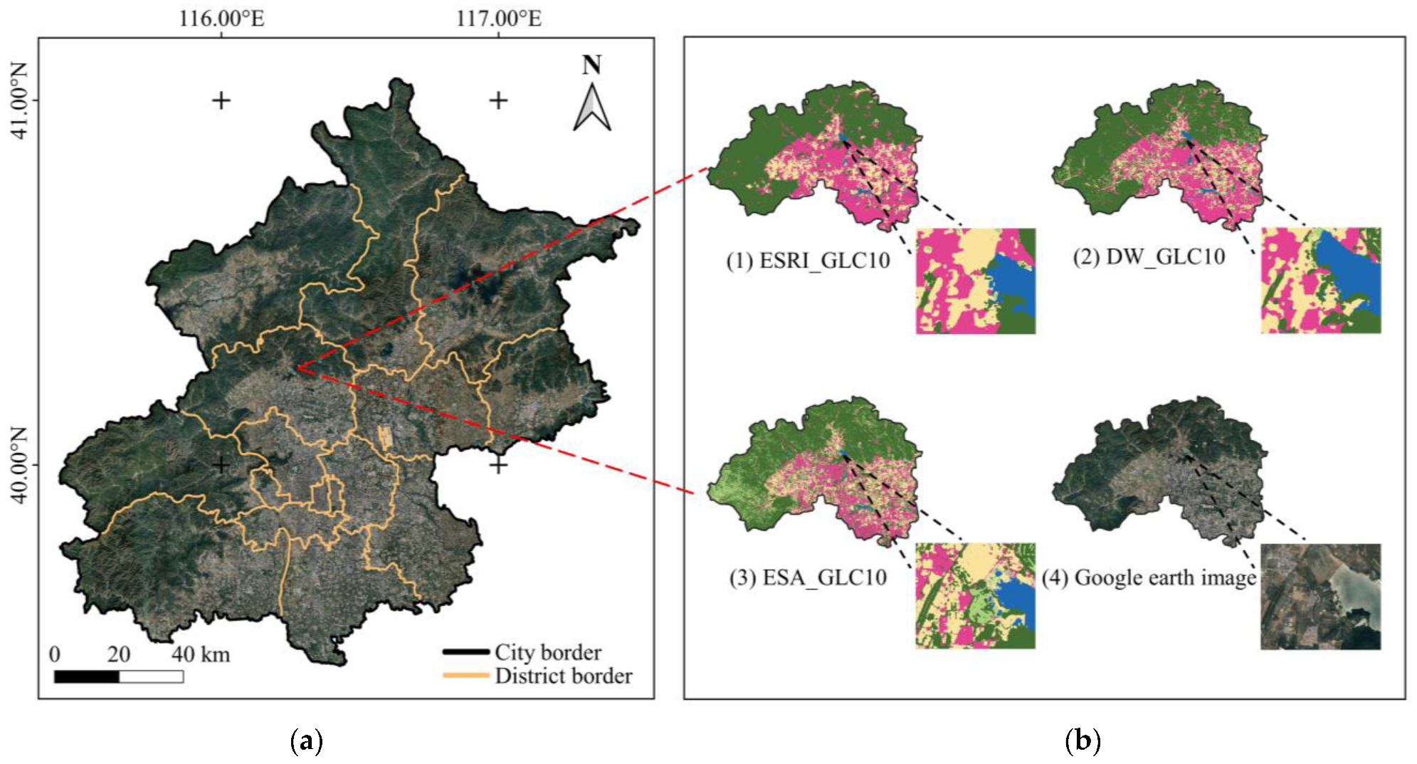
is an effective measure that overcomes the limitations of projection complexity. It can directly compute the difference between two-dimensional distributions. Therefore, in this study, it was employed to calculate the Wasserstein distance between LC products and the reference ground truth within the study area.
3.2. Wasserstein Similarity Index
This study divided the accuracy information carried by the LC products into two types: global feature information and spatial position information. Although the Wasserstein distance is effective in quantifying the similarity between products and the reference truth from a global feature perspective, its interpretability is affected because the total weight is evenly distributed among all pixels. Therefore, we normalized to ensure that the global feature similarity had a strict mathematical significance and was independent of the size of the study area.
The existence of target product A and reference truth B was assumed, whose matrix spaces are denoted as
and
, respectively. In the study area, there was a total of
land cover types, and the transformed numerical matrices satisfied
and
. Then,
can be defined as Equation (5).
where
represents the global feature similarity for the type
(
) in the study area, with
.
denoting the maximum centroid distance for the pixels of the land cover type
in A and B, which can be defined with Equation (6).
where
and
represent the pixels of the land cover type
in A and B, respectively.
denotes the centroid distance for the pixels of land cover type
in A and B. When the pixels in the two products are distributed in the diagonal corners of the area, the maximum centroid distance can be computed.
After considering the global feature information of the products comprehensively, there is also a need for an evaluation metric to assess spatial positional information. This study used the correlation coefficient to quantify the spatial position similarity between the target product and the reference truth. The correlation coefficient
can be defined with Equation (7), primarily reflecting the commonalities and differences in category composition between the product and the truth [
36].
Here, and represent the areas of type () for A and B, respectively. and are the average areas of each type in A and B, respectively within the study area.
With
and
serving as measures for different types of accuracy information, this study further introduced the Wasserstein similarity (WenSiM) between the target product A and reference truth B. The index comprehensively extracts accuracy information to reflect the overall similarity, and it is defined as follows:
where the
satisfies the condition
and
only when
, indicating that the target product and the reference truth are entirely identical in both spatial position and global features within the study area.
The WenSiM index fully takes use of more accuracy information to evaluate LC products. While maintaining properties such as symmetry, non-negativity, and identity, the WenSiM also possesses strict mathematical significance and interpretability. It is an excellent metric for accurately and rapidly assessing LC product accuracy. The detailed calculation process is summarized in Algorithm 1.
| Algorithm 1. (, , , , ) |
| 1: Initialize , |
| 2: Data preprocessing for , |
| 3: Repeat |
| 4: , |
| 5: |
| 6: |
| 7: |
| 8: |
| 9: |
| 10: Until |
| 11: |
| 12: Output |
3.3. Production of Validation Dataset
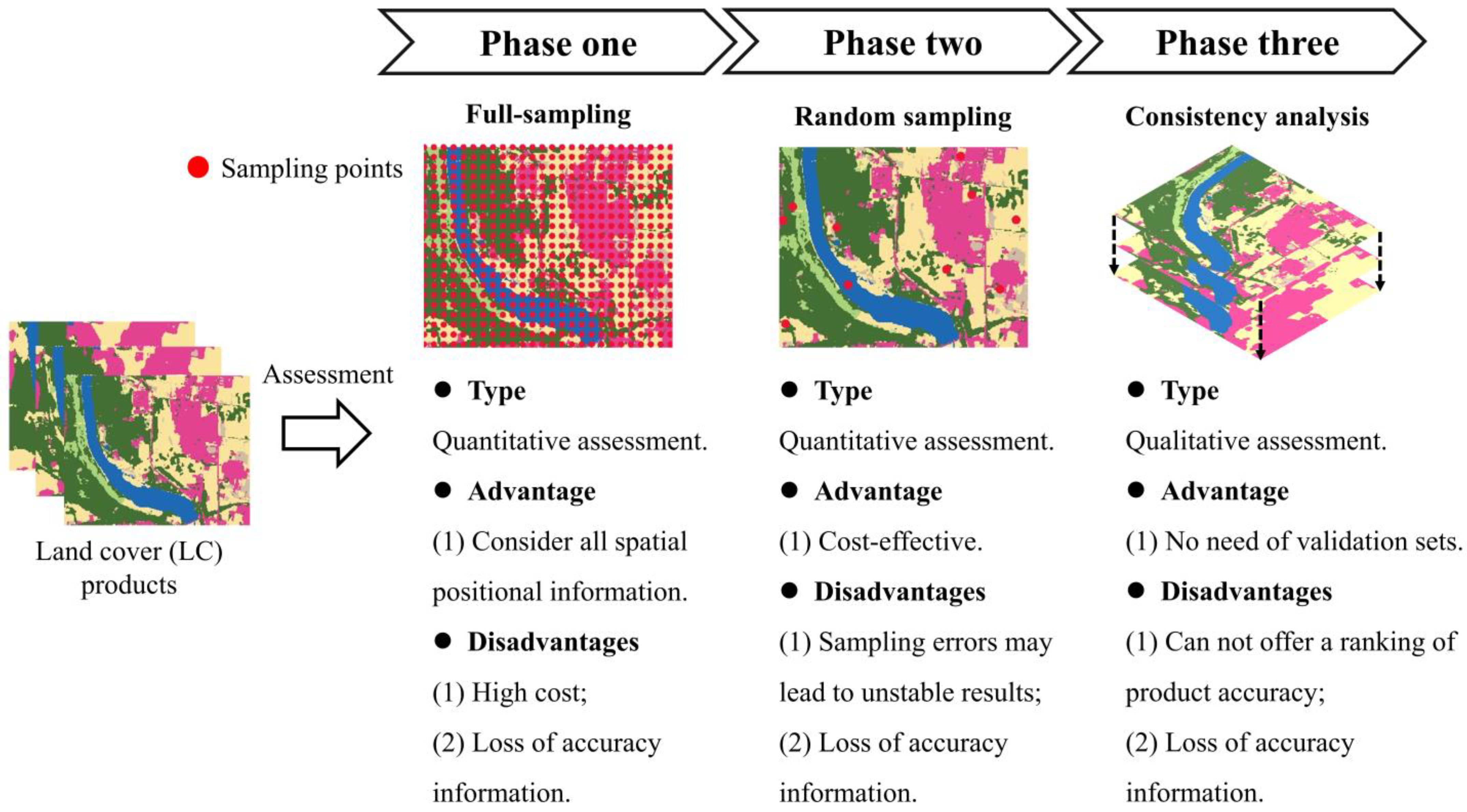
The evaluation method proposed in this paper can directly assess the accuracy of LC products without registration and validation datasets. In order to demonstrate the effectiveness and rationality of the WenSiM index, it is necessary to create a validation dataset to analyze the consistency between validation accuracy and assessment results.
Sampling is a crucial step in creating a validation dataset, as the sample size and sample variance determine the accuracy of the dataset. Although increasing the sample size is beneficial for improving accuracy, it also comes with the added cost of production. The optimal sampling scheme aims to obtain the most reliable validation results with the lowest cost [
37]. Therefore, once the sample size is determined, the key to improving the accuracy lies in reducing sample variance [
38].
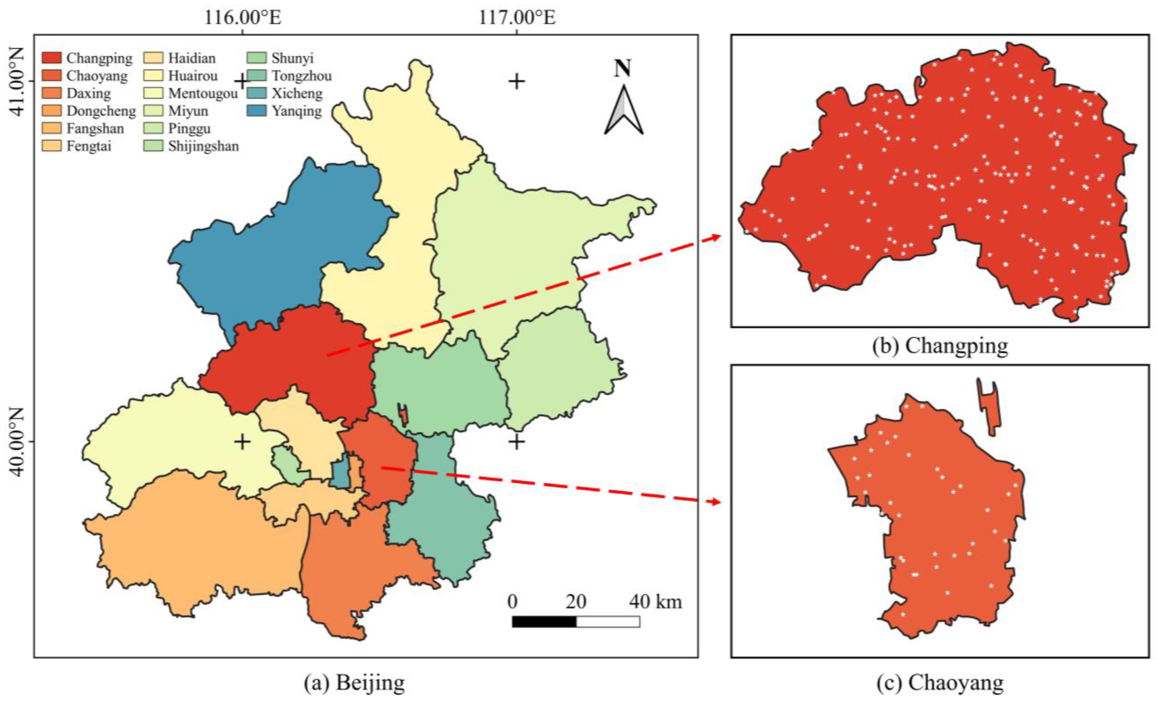
Stratified sampling (SS) is a great method to reduce variance and improve sampling accuracy when the sample size is constant [
39,
40]. To implement SS, it is crucial to confirm that every object in the sampling range shares similar properties. Subsequently, researchers can use a particular characteristic or rule to divide the population into
non-repeating sub-groups, each referred to as a layer. Finally, samples for each layer can be acquired through random sampling.
LC products possess both geographical and administrative attributes, allowing them to be divided into multiple levels using administrative boundaries. Therefore, researchers can divide the study area into
layers based on the characteristic. After getting sampling points through SS, an unbiased estimate of the variance
of all samples can be calculated by using Equation (9).
where
represents all samples, and
is the total population size.
and
are the weight parameter and the sampling ratio of layer
, respectively.
and
denote the number of samples and pixels in layer
, respectively;
is the sample mean of layer
; and the population variance of layer
can be written as
.
To minimize the objective function
, it is essential to choose an appropriate sample size and allocation method. This study adopted the Neyman optimal allocation method, which maximizes sampling accuracy by achieving a proportional distribution between
and
.
can be computed by Equation (10), where
is used to indicate the total number of samples.
The production method is based on SS theory and considers factors such as economic cost and sample quality, which involves scientifically selecting sample points to ensure that the accuracy meets research requirements. However, it is important to emphasize that the sample points selected through SS only reflect the spatial position information of the pixels and do not effectively reveal the global features formed by the pixels’ interactions.

 ,
, 
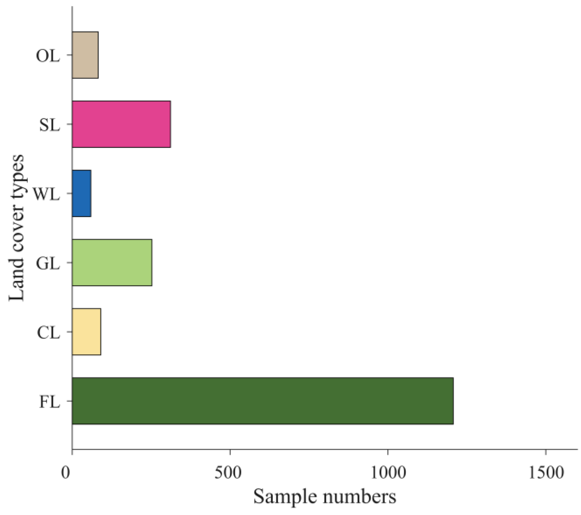
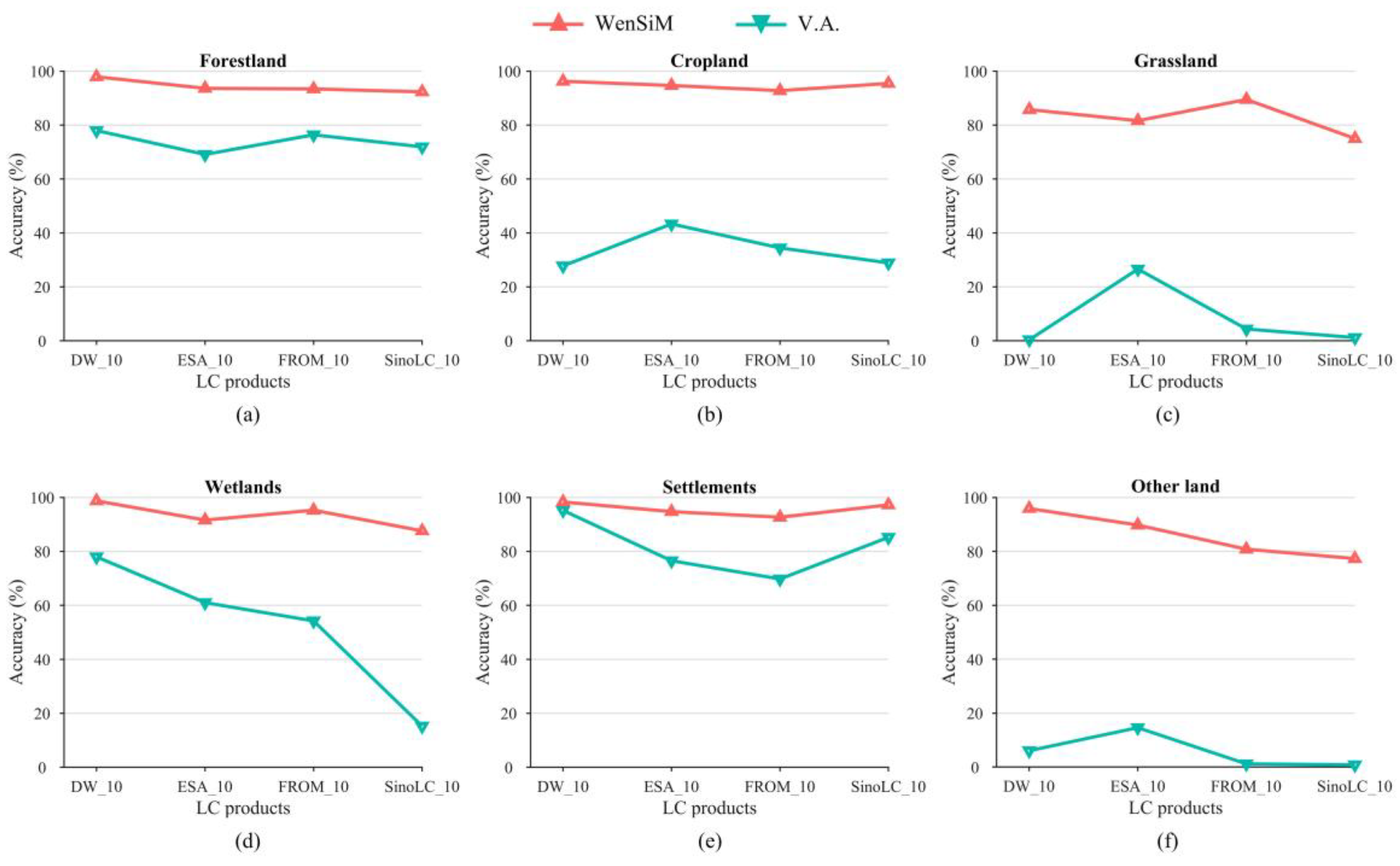
 Forestland
 Cropland
 Grassland
 Wetlands
 Settlements
 Other land


