DSSFN: A Dual-Stream Self-Attention Fusion Network for Effective Hyperspectral Image Classification

Abstract

Hyperspectral images possess a continuous and analogous spectral nature, enabling the classification of distinctive information by analyzing the subtle variations between adjacent spectra. Meanwhile, a hyperspectral dataset includes redundant and noisy information in addition to larger dimensions, which is the primary barrier preventing its use for land cover categorization. Despite the excellent feature extraction capability exhibited by convolutional neural networks, its efficacy is restricted by the constrained receptive field and the inability to acquire long-range features due to the limited size of the convolutional kernels. We construct a dual-stream self-attention fusion network (DSSFN) that combines spectral and spatial information in order to achieve the deep mining of global information via a self-attention mechanism. In addition, dimensionality reduction is required to reduce redundant data and eliminate noisy bands, hence enhancing the performance of hyperspectral classification. A unique band selection algorithm is proposed in this study. This algorithm, which is based on a sliding window grouped normalized matching filter for nearby bands (SWGMF), can minimize the dimensionality of the data while preserving the corresponding spectral information. Comprehensive experiments are carried out on four well-known hyperspectral datasets, where the proposed DSSFN achieves higher classification results in terms of overall accuracy (OA), average accuracy (AA), and kappa than previous approaches. A variety of trials verify the superiority and huge potential of DSSFN.

1. Introduction

With the advancement of space-borne remote sensing, the spectral resolution of satellite images has increased greatly. Compared to conventional remote sensing data, hyperspectral data offer a higher spectral resolution and more detailed feature information [1]. Various picture elements of different wavelengths can be subdivided and identified in spectral space based on factors such as spectral brightness, spatial structural attributes, or other information [2,3], as shown in Figure 1. Therefore, it is utilized extensively in urban planning [4], environmental monitoring [5], precision agriculture [6], forestry monitoring [7], ocean exploration [8], disaster monitoring [5,9], geological exploration [10], and even military applications [11]. Due to the limitations of the imaging technology, the sensor must generate a significant amount of redundant data in order to ensure an adequate exposure time and a reasonable energy for each band when developing hyperspectral data cubes, which adds to the storage and processing costs of the device [12]. During the analysis of hyperspectral data, not all bands are processed simultaneously. Instead, an ideal band combination is chosen, and band selection (BS) becomes necessary to preserve crucial information [13,14].

With minimal inter-band correlation and considerable spectral variability, the goal of band selection methods is to choose a subset of the original spectrum data based on specified criteria. These techniques not only resolve the potential dimensional catastrophe [15] brought on by the Hughes phenomenon, but they also maintain the physical significance of the original spectral bands and improve the interpretability of the resultant low-dimension features [16]. On the basis of their respective methodologies, hyperspectral band selection methods can be categorized as ranking-based, clustering-based, and search-based [17]. Methods based on sorting can pick subsets with a high degree of relevance. The clustering-based method may reduce data redundancy, while the combined approach can lessen the influence of noise bands on subsets of data. Sun et al. [18] proposed an adaptive band hierarchy (ADBH) clustering method and employed a band-based ranking strategy (E-FDPC). Wang et al. [19] introduced a fast neighborhood grouping BS method (FNGBS) that employs a coarse-to-fine grouping strategy for band clustering, minimizes redundancy, and ranks bands using the product of local density and information entropy. By the efficient band selection method, the original data’s spectral information is kept with greater interpretability and representativeness, thereby enhancing classification performance [20].

Classification is based on the fact that each pixel in the hyperspectral image (HSI) corresponds to a spectral curve representing optical and physical characteristics. The initial hyperspectral feature classification systems relied on empirical, subjective manual feature analysis. The support vector machines (SVM) [21] and k-nearest neighbors (K-NNs) [22] methods are two examples of machine learning techniques that were used for hyperspectral classification in the early stages of research. These methods are computationally straightforward and do not take advantage of the abundance of spatial information present in hyperspectral data, so they did not produce satisfactory classification results. Following the success of deep learning in computer vision, numerous deep learning classification approaches have been implemented in the hyperspectral image classification field. Chen et al. [23] classified hyperspectral pictures using stacked self-encoders, which marked the introduction of methods based on deep learning to the field of hyperspectral image classification. With its superior performance, convolutional neural networks (CNNs) are gradually becoming the method of choice for hyperspectral image categorization. The exiting research shows that feature extraction from shallow to deep plays a crucial role in the classification of hyperspectral images. CNNs often outperform other deep learning algorithms in feature extraction, primarily because their local connectivity and shared weight features enable them to learn spatial features while preserving the original structure and drastically lowering the number of network parameters [24]. In the early use of CNNs methods, only 1D [25], 2D [26], and 3D [27] convolutional neural networks were utilized for hyperspectral classification. Although the accuracy that can be attained with such simple forms of the approaches is restricted, this study presents ideas for future research on how to more effectively employ CNNs methods. Recent research has concentrated on determining how to use CNNs networks to effectively handle information in both spectral and spatial dimensions [28,29].

A traditional neural network typically consists of a single method for data processing, which can be conceptualized as a single stream. Dual-stream [30] neural networks were initially applied to human behavior recognition, wherein they were capable of concurrently processing two or more separate kinds of data. Xue et al. [31] used dual-stream network fusion to extract time-series features of different lengths and locations. Wan et al. [32] designed a parallel architecture to acquire independent spatial and channel dimensional information in order to generate more precise image captioning. This dual-stream concept is introduced to hyperspectral classification tasks in an effort to leverage the hidden information in the original data more efficiently. Zhang et al. [33] employed a 1-D CNN to extract spectral characteristics and a 2-D CNN to extract spatial-spectral features and then combined the features using a weighting mechanism to obtain excellent classification accuracy. Combining a CNN and a stacked denoising self-encoder, Hao et al. [34] suggested a dual-stream depth architecture. Using spectral picture components and spatial blobs, the categorization outcomes were predicted. Song et al. [35] developed a deep feature fusion network (DFFN) that fully exploits the complementarity between layers. To summarize these methodologies, researchers are continually attempting to determine how to combine spectral and spatial information more effectively. To extract spatial and spectral features, Cui et al. [36] developed a two-channel network structure. It also included a self-calibrating convolution module to capture the domain correlation of the context as the features were being extracted.

Despite the numerous CNN dual-stream hyperspectral image classification networks that have been proposed, these networks still suffer from the drawbacks of CNN models. For example, this method centers the network on sampling points and produces a patch of a fixed size while ignoring the scale information of HSI, where different features have different scales, and using the same size local patch inevitably results in poor classification of some feature categories. Because of this, the visual attention mechanism enables the network to choose the critical feature information on its own, reduces the impact of the irrelevant spatial information of the central pixel, and performs well in improving the final results of image classification. To effectively extract features, a 3D convolutional adaptive attention module for extracting joint spectral-spatial characteristics was initially developed in [37]. With the goal of extracting correlations and common spatial features in spectrum bands for the spectral and spatial attention components, respectively, Li et al. [38] proposed combining a spectral attention channel with a spatial attention channel. By merging various attention modules, Zhong et al. [39] were able to predict the relationships between spectral and spatial locations. The concept of integrating self-attention and adversarial attacks into hyperspectral image classification was initially proposed by Xu et al. [40], resulting in enhanced network robustness. Qing et al. [41] employed an improved three-dimensional multi-attention mechanism to concurrently handle the spatial spectral characteristics of hyperspectral images. Xia et al. [42] used a self-attentive approach to adaptive spatial feature fusion, a structure that employs a “divide and conquer” idea to reduce the number of model parameters and computations.

The attention mechanisms employed in hyperspectral classification approaches are integrated into the spectral and spatial information extraction network through stacking. Additionally, the multiscale extraction module is utilized to expand the perceptual field and deepen the layers of the CNN. However, this may result in a potential decline in performance. In light of this, we suggest a dual-stream classification network that leverages the self-attentive mechanism to capture spatial feature associations between the central pixel and its surrounding pixels. Furthermore, the network utilizes a residual pyramid structure to fully exploit the long-range correlation of spectral information for multi-scale feature extraction. Finally, the network achieves hyperspectral image classification through weighted fusion. The following are the primary contributions of this paper:

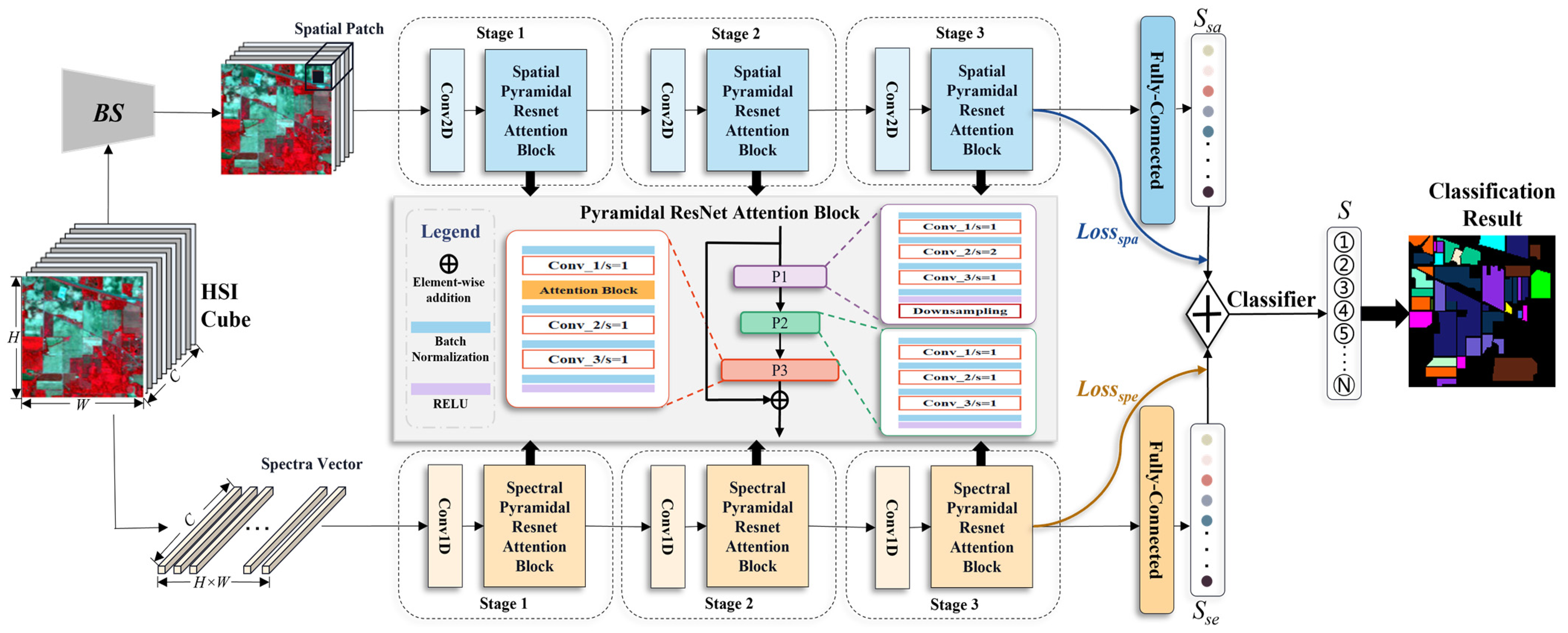
• A dual-stream hyperspectral classification network, DSSFN, is proposed. In comparison to the previous joint spectral-spatial network, not only does the self-attentive mechanism fully exploit the characteristics of hyperspectral data, but the pyramidal residual structure also achieves multi-scale feature extraction without deepening the network depth to generate high-quality feature discrimination results.
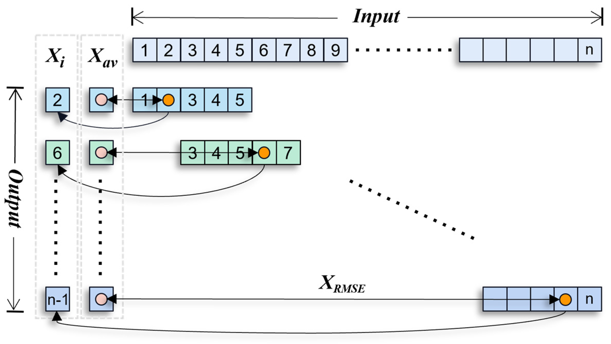
• To remove duplicate information in the original data, a novel sliding window-based band grouping method is adopted, and the matching filtering (MF)-based band sorting strategy is enhanced to further eliminate the influence of noisy bands and produce a more representative subset of bands.

The proposed method exhibits satisfactory hyperspectral image classification performance on four public datasets, which is highly competitive with other state-of-the-art methods. The remainder of this paper is organized as follows. Section 2 introduces the related basic approaches. Section 3 describes the dual-stream convolutional neural network and the self-attentive feature extraction module. Section 4 presents the experimental results and a discussion on the public dataset. Section 5 gives the conclusion.

2. The Basic Approach

This section presents an overview of the primary methodologies pertinent to the proposed approach, which are crucial for comprehending the entire network’s feature extraction process.

2.1. Hyperspectral Image Classification Based on CNNs

The hyperspectral data collected increasingly comprehensive information as imaging techniques advanced, producing greater data quantities and making data processing more challenging. Traditional classification methods can extract effective spectral features, but the linear simplicity of these models makes it challenging to deal with the complex spectral properties of classification [24]. In addition, misconceptions about high-dimensional and conventional space sometimes lead to a misinterpretation of HSI and inappropriate choices of data processing techniques [43]. As a subfield of machine learning, deep learning benefits from deeper networks, more sensors, and more neuron architectures. CNNs have the capability to accommodate various input data types, including one-dimensional (1D) vector data, two-dimensional (2D) planar data, and three-dimensional (3D) patterns. Unlike traditional neural networks, CNNs do not restrict the size of the input data, thereby enabling the network to learn from data of varying dimensions. These three characteristics are simultaneously present in hyperspectral data, with a 1D vector of data reflecting the value of a particular wavelength band above each pixel. Intercepting a 2D image enables the processing of each pixel’s surrounding class characteristics. 3D stereo data are the raw information of hyperspectral images. Figure 2 depicts the principle of the 1D,2D,3D convolution kernel for processing data of different dimensions.

Early 1D-CNN algorithms do not examine the spatial relationship of pixels and merely extract features based on spectral information, followed by end-to-end tuning. This method [24] requires more training samples and is challenging to implement in order to obtain the desired outcomes. CNNs are able to handle 2D images without altering the data’s original structure. Therefore, Liu et al. [44] recommended the use of 2D-CNN and demonstrated that the classification accuracy for hyperspectral images is much greater than that of 1D-CNN. Many traditional CNN designs, including AlexNet [45], have also been utilized for hyperspectral image categorization. However, the majority of CNN-based algorithms continue to extract spatial and spectral characteristics individually, making insufficient use of spatial and spectral correlation data. Li et al. [46] proposed using 3D-CNN in the classification of hyperspectral images, which can comprehend local variations in space and spectra and categorize them using crucial discriminative information. There remains potential for further optimization by employing a singular convolutional approach for classification. Hamida et al. [47] employed a fusion of 2D CNN and 3D CNN techniques, resulting in enhanced performance. However, the task of choosing the ideal number of network layers remains challenging. The effectiveness of image feature extraction is compromised when the neural network is either excessively deep or shallow. Therefore, the exploration of methods for optimizing the benefits of CNNs has become a prominent topic.

2.2. Band Selection Methods with Hyperspectral Images

The band selection methods can efficiently reduce the dimensions of hyperspectral data cubes while maintaining the pertinent feature information. The similarities between non-adjacent bands are typically less than those between neighboring bands because of the properties of hyperspectral data.

Several early band selection methods were developed to identify combinations of bands that preserved the best information. These methods included distance measures [48], information-theoretic approaches [49], and eigenanalysis methods [50]. One approach utilizes a divergence measure for hyperspectral band selection, requiring the computation of scatter for all band subsets. However, this task becomes considerably challenging when confronted with numerous bands in hyperspectral images [49]. Principal Component Analysis (PCA) is a method used for eigenanalysis in which the objective is to convert the original waveform data into a novel set of linear transformations that exhibit no correlation among themselves. To keep enough feature values, the feature amounts are ordered in descending order. Although the pixel information of hyperspectral images is preserved in this manner, the similarity and correlation between nearby spectra are not considered. In [51], spectral subsets are chosen by thresholding, which is substantially correlated with the classification performance, and hyperspectral data are separated by correlation generation curves of adjacent spectral bands. Through the application of a dynamic planning approach, the data were divided to produce the same performance improvement [52]. The clustering method selects all cluster centers and combines closely related bands into a single subset. However, this method disregards the data content [53,54]. In contrast to clustering methods, sorting methods quantify and rank the physical data of frequency bands. To produce subsets, the frequency bands with greater weights are selected [55,56]. Clustering- and sorting-based approaches by themselves frequently result in redundant band information. The integration of sorting and clustering methodologies facilitates the reduction in dimensionality in high-dimensional datasets [57].

For the neural network calculation to choose the hyperspectral subsets with more information and a lower correlation between bands, the data after dimension reduction will be advantageous. The selection of spectral subspace bands begins with the subdivision of subspaces, and the number and expression of subspaces are critical to the final outcome. Mathematical calculations can be employed to determine a strong correlation using coefficients.

2.3. Self-Attention in the Transformer

The previously mentioned convolutional neural network approaches for hyperspectral data feature extraction include flatness and learning consistency. These networks cannot fully take advantage of the medium- and long-range information in the spectrum dimension due to their low capacity for continuous spectral data. A CNN relies largely on the size of the convolution kernel to extract features; therefore, dilated convolution [58] is developed to pursue a bigger perceptual field. Nevertheless, the performance attained in this manner is restricted and cannot handle regions with arbitrary shapes.

The integration of the “attention mechanism” [59] imbues machines with human-like perceptual capabilities, enabling them to learn and identify the most pertinent regions within hyperspectral data. When applying this approach to neural networks, retrieved features can be better characterized. The self-attentive mechanism-based structure of Transformer is adaptable and easy to generalize. Transformer was initially implemented for natural language processing (NLP). The spectral vectors resemble the distribution of semantic vectors for words. The spatial classification of hyperspectral data requires the use of neighboring pixels inside the input region [60,61,62].

The principles of the self-attention mechanism and the multi-head attention mechanism are depicted in Figure 3.

Dosovitskiy et al. [63] introduced Vision Transformer (ViT) for image classification, which progressively analyzes picture patches using a self-attention (SA) transformer encoder with positional embedding. Transformer, which applies the ViT structure to the classification of hyperspectral images, has a global feature domain and thus collects more global background information. This is accomplished through a multi-headed self-focus mechanism. Transformer can be used to classify HSIs in multiple ways. He et al. [64] created a spatial spectral converter that uses a CNN to record spatial information and ViT to extract spectral relationships. For capturing at greater distances, Qing et al. [65] added a position encoding vector and learnable embedding vector to the network. Hong et al. [60] proposed the SpectralFormer structure, which is also capable of learning spectral local sequence information from adjacent bands of hyperspectral pictures in order to group the spectral structure. In general, the success and adaptability of transformers’ structures rely greatly on the application of the multi-headed attention mechanism. The weighted total of sensory fields can be represented by both convolution and self-attention methods. Convolution ensures the most robust response of local features and decreases the model’s complexity, while the self-attention method can directly capture global information and calculate weights by normalizing pairwise information. The combination of the self-attention mechanism and convolutional network can facilitate the preservation of desired hyperspectral characteristics and also reduce the computational expenses [66] associated with the model simultaneously.

2.4. Pyramidal Residual Networks

For the vast majority of deep convolutional neural networks [67,68], the dimension of the feature map grows as its size decreases. Nevertheless, it is exceedingly difficult to train very deep convolutional neural networks using hyperspectral data. This is due to the unavoidable loss of information caused by the elimination of gradients, which makes propagation less effective and accuracy plummet.

The appearance of ResNet [67] resolves this issue. A residual block is comparable to a top-down connection between each layer and a jump connection between units. Each module in ResNet has the same structure and completes the aggregation at the output layer. Thus, each block carries out an identical feature extraction operation. And yet, this residual structure of preserving the dimensions is not the most effective; for example, the PyramidNets [69] employs a structure that gradually increases the channel dimensions. In the pyramidal residual units, zero-padded identity-mapping short-cuts [67] are employed because establishing too many 1 × 1 convolution blocks can have a negative impact on performance. The various widths of each rectangular module in Figure 4 stand in for various input feature map dimensions for the current module.

According to the experimental results in references [68,69], the pyramid residual network attempts to progressively expand the dimension of the feature map rather than doubling it over a residual unit. This equally shares the burden of expanding the feature map. Comparing PyramidNet to the pre-activated ResNet, the overall performance is enhanced. The PyramidNet has a greater test accuracy with the same settings, indicating its superior generalization ability compared to existing deep neural networks. This method has no parameters and a decreased likelihood of overfitting than other forms of shortcuts, resulting in enhanced generalization capabilities. The main concept is to concentrate attention by gradually increasing the dimension of the feature map, as opposed to downsampling by drastically increasing the dimension of the feature map on each residual unit. The connection between the several residual modules creates a pyramid structure with the feature map’s dimension continuously growing. In conclusion, it is ideal for extracting hyperspectral data features.

3. DSSFN: High-Performance Feature Extraction

In this section, the nearest neighbor grouped normalized matching filter, the dual-stream convolutional neural network, and the self-attentive mechanism are described in detail. Figure 5 illustrates the proposed DSSFN network.

3.1. Sliding Window Grouped Normalized Matched Filter

Suppose $X=\left\{X_k\mid X_1,X_2,X_3,X_4\dots \dots .X_n,k=1,2,3\dots \dots ,n\right\}$ is a hyperspectral image to be processed, where n is the total number of bands and $X_k$ is the vector of the k band. In order to derive characteristic spectral bands, an initial subspace comprising m relevant bands, ranging from band $X_1$ to the $X_m$, is defined. The representative bands within this subspace are then identified based on their deviation from the mean band, which serves as a statistical parameter for measuring inter-spectral similarity. This can be mathematically expressed as:

$$X_{RMSE}=\sqrt{\frac{{\left(X_i-X_{av}\right)}^2}{N}}$$

(1)

where $X_i$ represents each band, $X_{av}$ represents the average band, and $N$ denotes the quantity of pixel points present on every band feature map. $X_{RMSE}$ is the correlation coefficient with the average band, and the smaller the correlation coefficient, the stronger the correlation. In the first subspace, the representative band is selected as $X_i$, and then the second subspace is selected as m bands from $X_{i+1}$ to $X_{i+m}$, and the similarity between bands is calculated as described previously, and so on, until all bands have been traversed. A considerable number of trials demonstrate the existence of an optimal value range for m. It is appropriate to set m to 5 as the sliding band group’s window size. Figure 6 depicts the dimension reduction algorithm’s procedure.

After the first stage of coarse dimension reduction is completed by nearest neighborhood subspace band selection, the second stage of dimension reduction consists of automatically removing poor bands from the scene using multiple target matching filtering (MF) weights. Relative to the direct normalization of the original data, the subsets normalized after coarse dimension reduction are more conductive to band distinction because they dramatically minimize inter-spectral disparities.

Assuming that the reduced-dimensional ${\mathit{x}}_{\mathit{i}\mathit{j}}^{\mathit{k}}$ represents each target pixel of band k, the corresponding formula for calculating the weight ${\mathit{w}}_{\mathit{i}\mathit{j}}^{\mathit{k}}$ can be expressed through the MF detector as:

$$\begin{gathered} {\mathit{w}}_{\mathit{i}\mathit{j}}^{\mathit{k}}=\kappa {\mathit{K}}^{-1}\left({\mathit{x}}_{\mathit{i}\mathit{j}}^{\mathit{k}}-{\mathit{m}}^{\mathit{k}}\right) \\ \left(i=1\dots \dots W; j=1\dots \dots H; k=1\dots \dots n\right) \end{gathered}$$

(2)

where ${\mathit{m}}^{\mathit{k}}$ is the mean value of each pixel in the k band, and i and j denote the coordinate position of this pixel in the k band.

$$\kappa =\frac{1}{\left[{({\mathit{x}}_{\mathit{i}\mathit{j}}^{\mathit{k}}-{\mathit{m}}^{\mathit{k}})}^T{K}^{-1}\left({\mathit{x}}_{\mathit{i}\mathit{j}}^{\mathit{k}}-{\mathit{m}}^{\mathit{k}}\right)\right]}$$

(3)

where K is the covariance matrix, and κ represents the normalization constant. The weights of each band are obtained by calculating the mean of the absolute weight vectors.

$${\left|w^k\right|}_{\mathrm{mean}}=\frac{1}{WH}{\displaystyle \sum }_{ij=1}^{WH}\left|w_{ij}^k\right|\in {ℝ}^{B_i\times 1}$$

(4)

where ${\left|w^k\right|}_{\mathrm{mean}}$ denotes the corresponding weight vector of band k, and WH represents the width and height of the feature map. The bands with greater weights are deemed to have a stronger signal-to-noise ratio and image quality, whereas the bands with lower weights may contain potentially degraded information. The desired number of bands is therefore determined by the weight ordering.

3.2. Dual-Stream Convolutional Neural Network

To enhance the fusion of spatial and spectral attributes in hyperspectral data, we introduce a dual-stream neural network for feature extraction. This network comprises a spectral stream, which processes a 1D spectral curve, and an image stream that performs spatial feature extraction using a reduced-dimensional processed image as the input. The dual-stream network offers a unique advantage in that it enables the utilization of distinct and non-shared structures and parameters in each of its branches, with no interference from back propagation. This enables the extraction of features with varying dimensions from a single-source dataset, which can subsequently be fused to produce complementary features, resulting in a significant enhancement of recognition rates. In addition, it may employ different types of inputs for feature extraction, which is versatile, leverages the benefits of the network structure, and can improve the network model’s understanding of the features. In the spatially based classification method, the raw hyperspectral data stream in the model is initially preprocessed by using the dimension reduction methods mentioned above. From the original images, pixels and neighboring regions are extracted as input modules for convolutional neural network processing to derive spatial feature representations. We present a residual network with a pyramidal structure, inspired by [70], in which each pyramidal residual block is constructed of three convolutional cells of varying sizes. The main concept is to gradually increase the number of channels on each cell by gradually increasing the feature mapping dimension, as opposed to quickly raising the feature mapping dimension through downsampling. When the depth of the leftover cells increases, additional feature mappings can be retrieved, allowing a more robust spatial feature representation to be learned from the image blocks. In addition, a batch normalization layer (BN) [71] is added to the pyramid residual network to improve the network generalization ability and prevent the occurrence of overfitting. To create a pyramid-like structure in Figure 5, P1, P2, and P3 indicate three cascaded residual units with progressively more feature map channels per unit. The cascaded pyramidal residual network cannot be classified effectively using hyperspectral data that have been directly translated. After band selection, we continue modifying the pyramid residual block structure to increase the accuracy of the classification of the hyperspectral data. Specifically, we have introduced a self-attention mechanism to replace one of its constituent layers, which has been found to significantly improve the effectiveness of the classification process. Further elucidation of the self-attention module is presented in the subsequent section. The network for spatial feature extraction consists of a stack of three identical pyramid residual modules, each of which can be characterized as BN1–CONV1–BN2–CONV2–BN3–SA–RELU, where SA is a self-attention module. Labelled numbers are used to distinguish between convolutional layers of various sizes and batch normalization layers. The output of the entire residual network module for a pyramid can be stated as:

$$Y=Relu\left\{zero\left(P_i\right)+\left[BN\left(P_i\right)\ast W_i+b_i\right]\right\}$$

(5)

where zero( ) is the constant jump mapping with zero padding, $W_i$ is the weight matrix, and $b_i$ is the convolutional layer bias.

The spectral-based classification approach varies from the spatial feature extraction network in that the dimensions of the convolution kernels for the spectral stream are 1D-CNN, and for the spatial stream, they are 2D-CNN. After the final pyramid residual module, the average pooling layer is configured for the final downsampling operation, which is then delivered to the fully connected layer to finish the classification task.

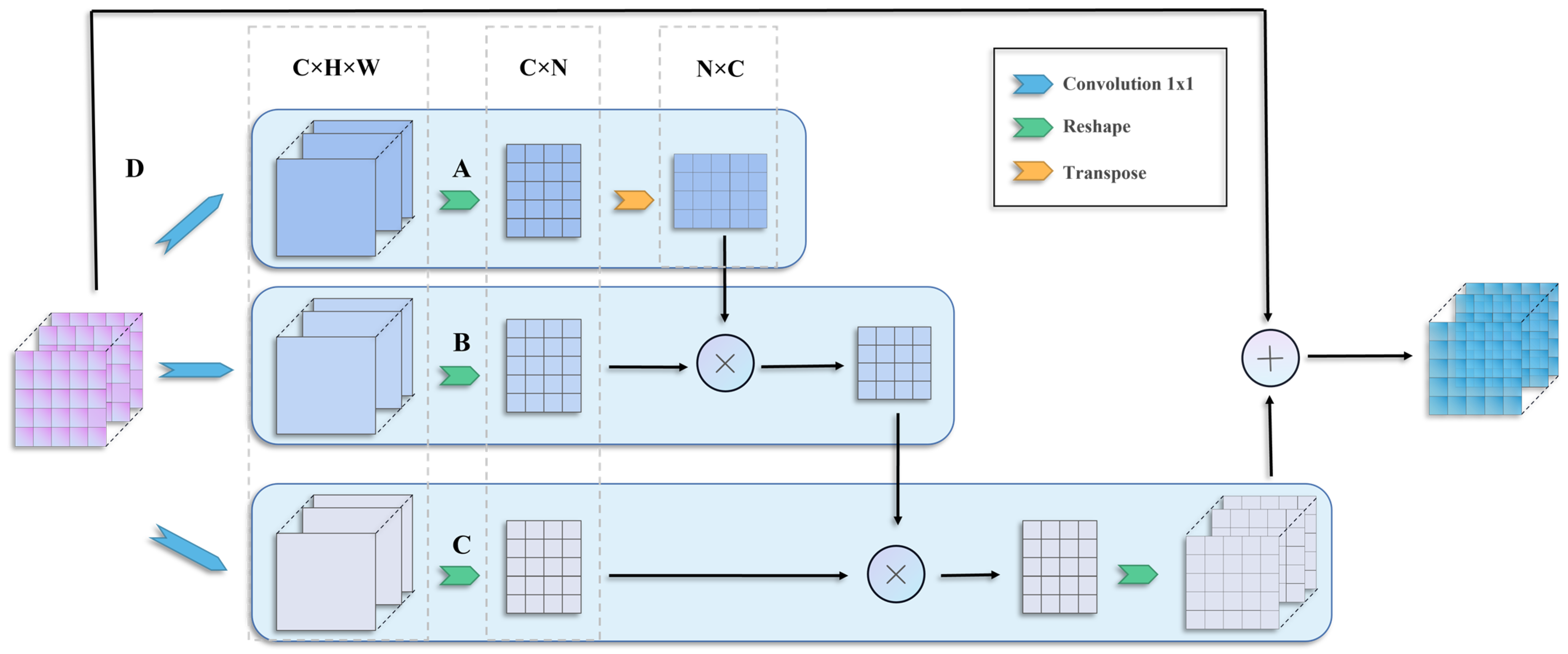
3.3. Self-Attention Mechanism

Due to the typical constraint on the size of each convolution kernel within the network, every operation is limited to a small region surrounding a specific feature point. As a result, capturing distant features becomes a challenging task. Self-Attention is adopted to retrieve global features more quickly by directly computing the relationship between any two-pixel spots in the feature map, hence addressing the aforementioned flaws. Figure 7 depicts the implementation sequence of the self-attention mechanism described in this article.

Imagine the constituent pieces of the input source information as a set of <Key, Value> data pairs and then calculate the similarity between the Query and each Key value for a given element of the target information. The weight coefficients of the Value values corresponding to each Key are determined, and then the Values are weighted and totaled to provide the final Attention values. Self-Attention is a specialized attention mechanism that computes attention on the sequence itself and gives different weight information to distinct elements in order to determine the sequence’s link. Self-attention can effectively improve the representation of global features with fewer parameters.

Spatial and spectral self-attention modules are created by linking this characteristic with pyramidal residual networks. In the spatial self-attention module, patch is first fed into two 1 × 1 convolution layers to produce two new feature maps B and C for $\left\{B,C\right\}\in {ℝ}^{C\times H\times W}$, respectively, and then we change its size to ${ℝ}^{C\times N}$, $N=H\times W$ being the total number of input pixels. Subsequently, a matrix multiplication operation is conducted between the transpose of C and B, followed by normalization to obtain the spatial self-attention weight distribution $S\in {ℝ}^{N\times N}$.

$$s_{ji}=\frac{\mathit{exp}\left(B_i\cdot C_j\right)}{{{\displaystyle \sum }}_{i=1}^N\mathit{exp}\left(B_i\cdot C_j\right)}$$

(6)

where $s_{ji}$ denotes the influence of the i position on the j position, and the more similar the features of the two positions, the stronger the correlation between them. At the same time, we input the feature map A to the convolution layer, generate a new feature map $D\in {ℝ}^{C\times H\times W}$, and change its size to ${ℝ}^{C\times N}$. Then, matrix multiplication is performed between D and the transpose of S, yielding a result of size ${ℝ}^{C\times H\times W}$, which is fed into a weight parameter $\omega$ at the end of the module. The outcome of the multiplication operation is then multiplied with $\omega$ and added to A. The formula is as follows:

$$E=\omega {\displaystyle \sum }_{i=1}^N\left(s_{ji}{D}_i\right)+A_j$$

(7)

where $\omega$ is initialized to 0 and is engaged in the learning and updating of the network. From the formula, it is known that E is the weighted sum of the features computed for all locations and the original features of the input. Thus, it has global contextual relations and selectively aggregates contextual information according to the spatial self-attentive weight distribution matrix.

In spectral attention, the input of the module is $A\in {ℝ}^{C\times H\times W}$. Unlike the spatial self-attention mechanism, the self-attention distribution is calculated directly from the original features. This involves transforming the size of $A$ into ${ℝ}^{C\times N}$ and multiplying $A$ with its transpose. The weight distribution $X\in {ℝ}^{C\times C}$ is obtained by normalization. The formula is as follows:

$$X_{ji}=\frac{\mathit{exp}\left(A_i\cdot A_j\right)}{{{\displaystyle \sum }}_{i=1}^c\mathit{exp}\left(A_i\cdot A_j\right)}$$

(8)

where $X_{ji}$ calculates the effect of the i spectrum on the j spectrum.

A matrix multiplication is performed between the transpose of $X$ and $A$, resulting in a matrix of size ${ℝ}^{C\times H\times W}$, which is then multiplied by a weight parameter and added pixel by pixel to $A$ to generate the final matrix representing the spectral self-attention weight distribution, as given in Equation (9).

$$E_j=\rho {\displaystyle \sum }_{i=1}^C\left(x_{ji}{A}_i\right)+A_j$$

(9)

where $\rho$ gradually learns the weights from 0 as the network is updated.

Modeling the lengthy dependencies between the feature maps yields the last feature of each channel, which is the sum of all spectral channel features weighted with the original features. It can assist in enhancing the discriminative quality of the characteristics. Therefore, the spectral self-attention module does not employ the convolutional layer to embed features before calculating the weight distribution of the relationship between two spectral channels. In Section 4, the experiments and validation will be presented and discussed.

3.4. Fusion Weighted Mechanism

While extracting features, the entire image is sliced into small portions and sent to the network for training. The independent extraction of each pixel slice is warranted due to the limitations of the fully connected layer employed in the neural network, which fails to incorporate positional information present in the convolutional layer. The single-label output generated upon the input of an image to the network precludes a pixel-level classification of the entire image. Thus, the discrete extraction of each pixel slice is deemed essential. The exiting research of dual-stream convolutional neural network fusion [72] demonstrates that fusing the recognition results to identify the proper rate is superior to fusing them in the process. Multiple fusion with full connectivity and the final convolutional layer is one of the better methods; however, the estimated parameters will be doubled, and the accuracy will increase by just 1.7%. In this research, we emulate the notion of integration learning in machine learning by using several weak-based learners for dataset learning and then merging the learners to obtain a higher performance by fusing the recognition results. The spectral and picture channels are learned independently, and the identification rate is enhanced by employing a weighted fusion method based on their properties.

An adaptive feature combination technique is presented in this paper, which aims to efficiently integrate pixel and channel features. The output of the fully connected layer is the feature vector obtained after two branches, whose length is equal to the number of data categories. Taking inspiration from reference [73], the approach we adopt for the fusion weighting of two-stream networks involves the use of score weighting. Separately, the weight matrices $W_{se}$ and $W_{sa}$ for spectral and spatial dimensions are learned, corresponding to the joint scoring of features $S_{se}$ and $S_{sa}$ to obtain the resultant vector $S$. This procedure can be stated as:

$$S_{se}=F_{se}\ast W_{se}$$

(10)

$$S_{sa}=F_{sa}\ast W_{sa}$$

(11)

If $S_{se}$ and $S_{sa}$ are directly summed, the different importance of the two parts is not emphasized. This is equivalent to feature splicing with an equal weight, which does not demonstrate good performance and may have harmful repercussions. During the process of training the network, a number of parameters are gathered in order to adaptively determine the ratio of the space to the spectrum. This can be viewed as an improved variant of feature stitching, and the processed model will have a more robust data representation than channel stitching and feature weighting. The process of adaptation can be described as follows:

$$S=\alpha \ast S_{se}+\beta \ast S_{sa}$$

(12)

$\alpha$ and $\beta$ are represented here as the reciprocal of the loss values produced during network training by the cross-loss entropy loss function. The loss value is the distance between the predicted value and the previous label. The smaller the loss value, the closer the distribution of the two variables, and the greater the model’s performance.

To optimize the above-given model, a suitable objective function is needed. Cross entropy is commonly used loss function for the classification problems. Here, we also use the cross entropy as a loss function of DSSFN for the classification of HSI. The loss function for cross entropy is given as follows:

$$Loss=-\frac{1}{M}{\displaystyle \sum }_{m=1}^M{\displaystyle \sum }_{c=1}^C{y}_c^m\mathit{log}(\overline{y_c^m})$$

(13)

where $y$ and $\overline{y}$ are the truth and predict labels, respectively. C is the number of classes, and M is the number of samples in a minibatch. The parameters in the model are updated by backpropagation and stochastic gradient descent.

In the experiments, the training and test sets are chosen by seeding the fixed spectral flow with the spatial flow at random. In addition, the spectral dimension is trained using the spectral profile of each pixel point, and the spatial dimension is focused on the target pixel using the same training sample and comparable loss.

4. Experimental Results

In this section, the proposed method is qualitatively and quantitatively evaluated using four hyperspectral public datasets, including the Salinas Scene (SA), Pavia University (PU), Kennedy Space Center (KSC), and Indian Pines (IP) datasets.

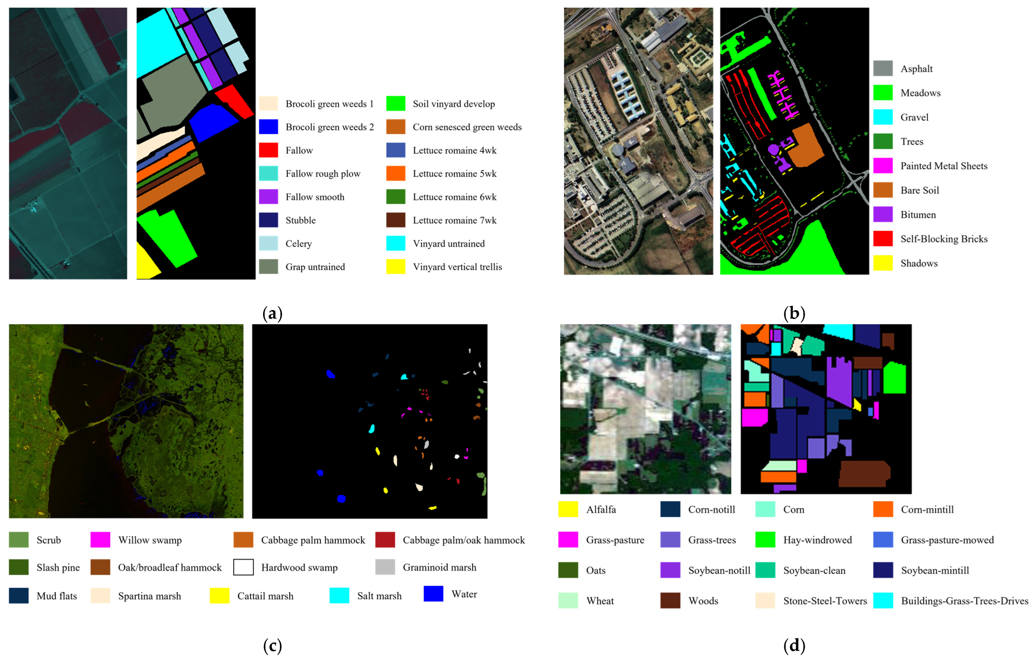
4.1. Dataset Description

Salinas Scene (SA): This dataset was collected by the Airborne Visible Infrared Imaging Spectrometer (AVIRIS) [74], over the Salinas Valley, California, USA. It includes 224 spectral bands with 512 × 217 pixels. After removing the bands with a low signal-to-noise ratio (SNR), 204 bands with a spatial resolution of 3.7 m/pixel remain. There are a total of sixteen classes of features covered.

Pavia University (PU): The dataset was collected by the Reflection Optical System Imaging Spectrometer (ROSIS) [75], over the urban region surrounding the University of Pavia in northern Italy. It includes 115 spectral bands with 610 × 340 pixels. It features a spatial resolution of 1.3 m/pixel and a spectral resolution of 4 nm in the range of 0.43~0.86 μm. There are a total of nine classes of features, and after deleting 12 noisy bands, the classification of this paper is based on the remaining 103 bands.

Kennedy Space Center (KSC): The dataset was collected by the NASA Airborne Visible/Infrared Imaging Spectrometer (AVIRIS) [74] over the Kennedy Space Center in Florida, USA. It boasts a spatial resolution of 18 m/pixel and a spectral resolution of 10 nm in the range of 0.4~2.5 μm. There are thirteen feature classes available. After deleting the absorbance and poor SNR bands, the classification of this work is based on the remaining 176 bands.

Indian Pines (IP): The dataset was collected by the Airborne Visible/Infrared Imaging Spectrometer (AVIRIS) [75] sensor over the Indian Pines Proving Ground in northwest Indiana. It consists of 224 spectral bands and 145 × 145 pixels. It has a spectral resolution of 10 nm, a range of 0.4~2.5 μm, and a spatial resolution of 20 m/pixel. There are sixteen feature classes available, and after deleting 20 bands spanning the absorption region and 4 zero bands, 200 bands are used for categorization.

Figure 8 depicts the pseudo-color composites of the mentioned four public datasets and their corresponding ground reference data.

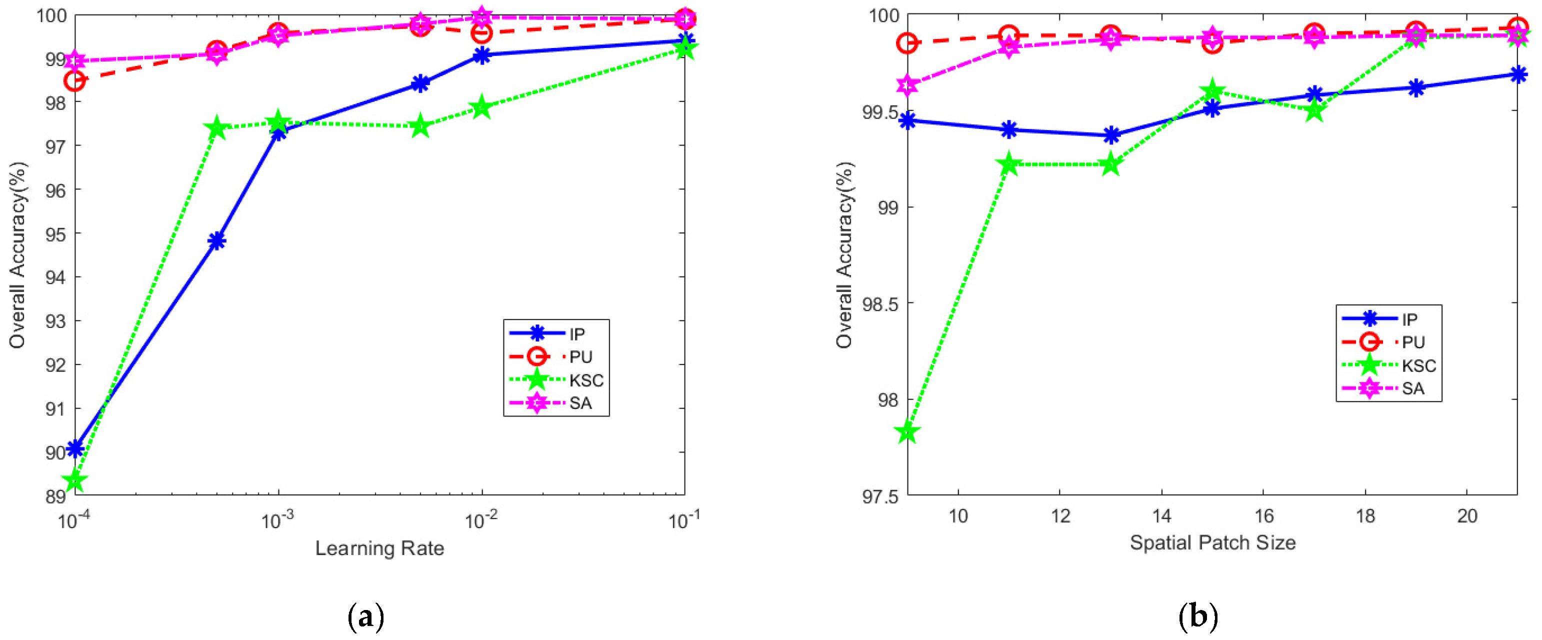
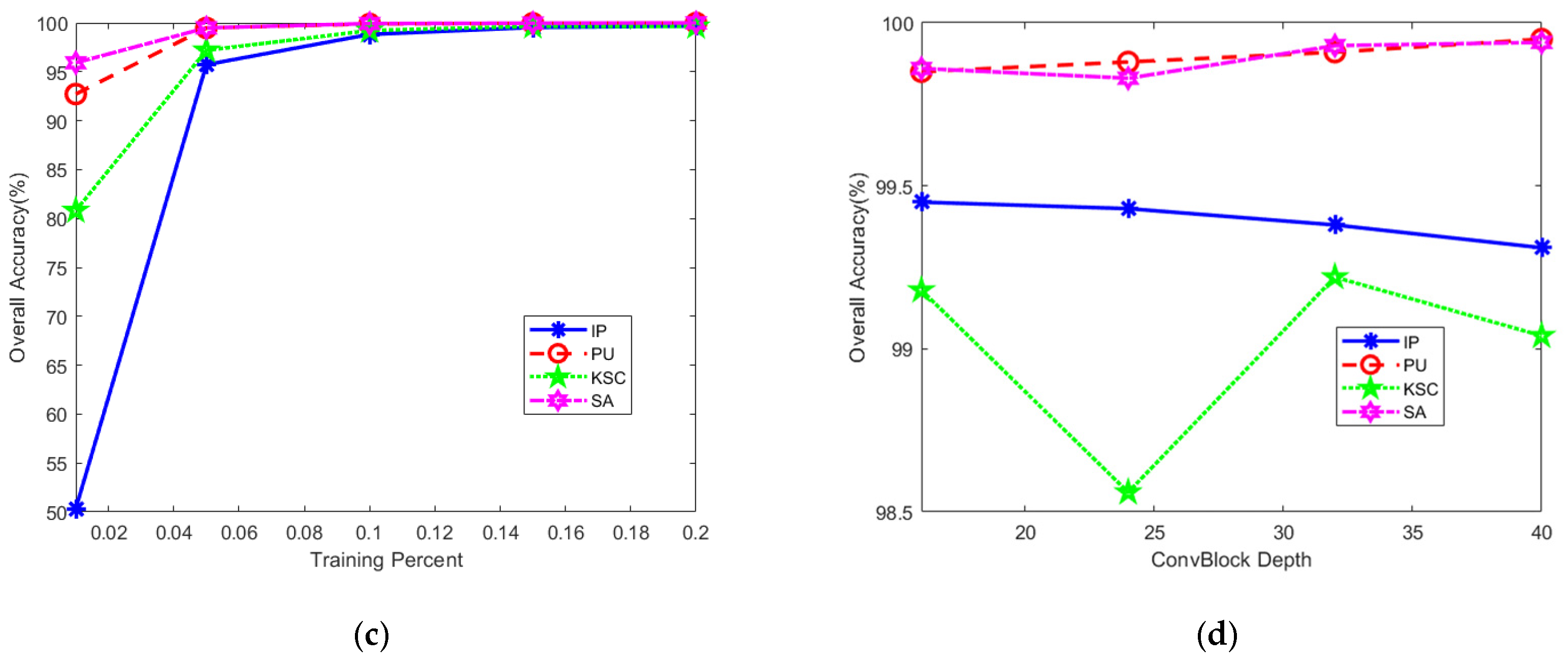
4.2. Parameter Settings

Experiments are conducted on a Linux system with Python 3.8 and four NVIDIA GeForce RTX 3090 GPUs in order to evaluate the performance of the proposed DSSFN model. As quantitative evaluation measures for the proposed method, we use the category accuracy, overall accuracy (OA), average accuracy (AA), and kappa coefficient (κ). The size of the spatial input, depth of the convolutional block, percentage of training set samples, number of spatial self-attention feature extraction layers, and learning rate are all analyzed, as they have an impact on the training progress and classification performance of the trained DSSFN network.

A specific percentage of samples is randomly chosen from each category individually to form the training set, while the remaining samples are designated as the test set. A spectral patch is comprised of a curve associated with each individual pixel point. When we make the spatial patches, the region surrounding the pixels of the labeled samples is divided into patches. In contrast to the prevalent random approach employed in hyperspectral classification, our methodology involves utilizing neighboring sliced pixel points as training data. In the context of training a model, the utilization of completely random sampling often results in the exposure of certain test samples to the model. This phenomenon may lead to excessively positive outcomes when evaluating the test dataset. Furthermore, the use of completely random sampling is not feasible in practical scenarios. The difference arises due to the typical practice of selecting training and test samples from separate locations [76].

For each combination of the aforementioned hyperparameters, the model with the best classification performance on the test set is retained on each dataset for a comparison with other experimental methods. A batch size of 16 is utilized, and each experiment is run for 300 iterations, given the number of training samples. Figure 9 shows the classification precision of OA values on each dataset based on different hyperparameter settings.

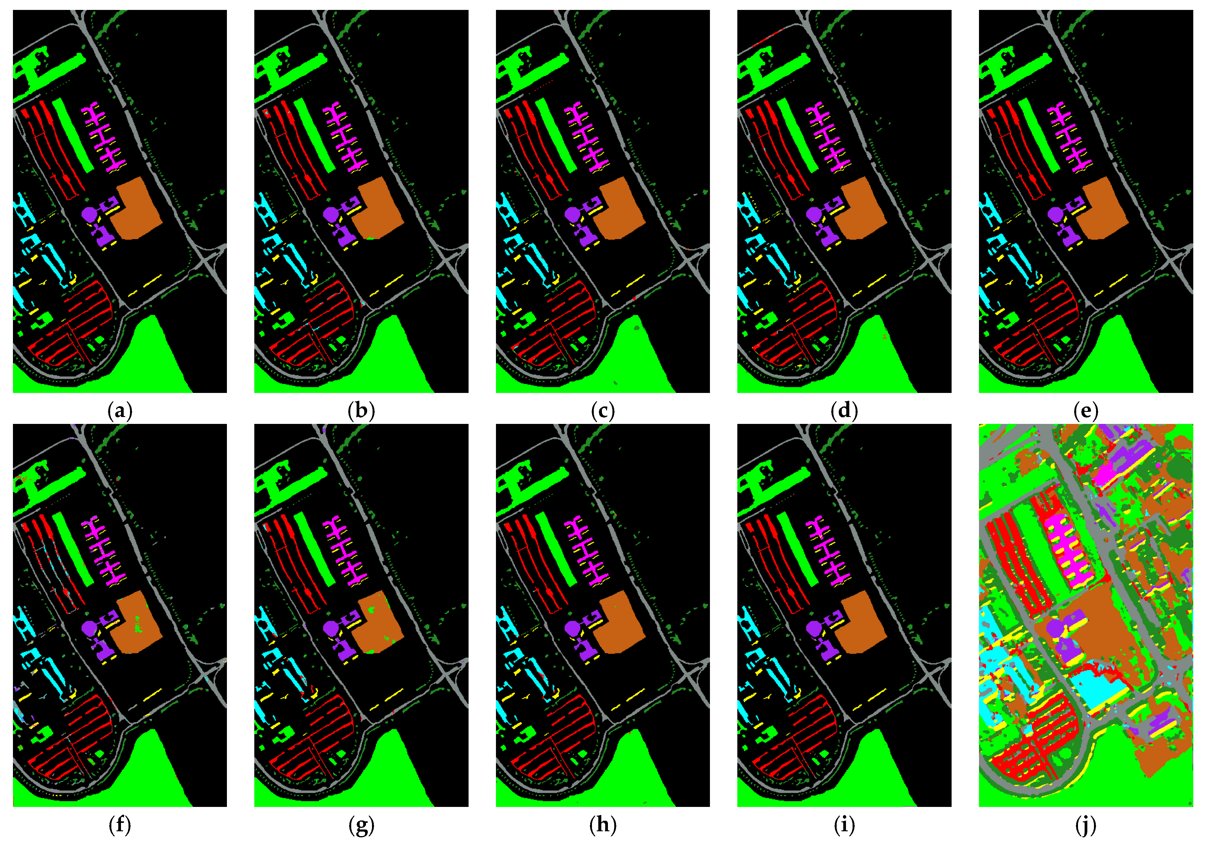
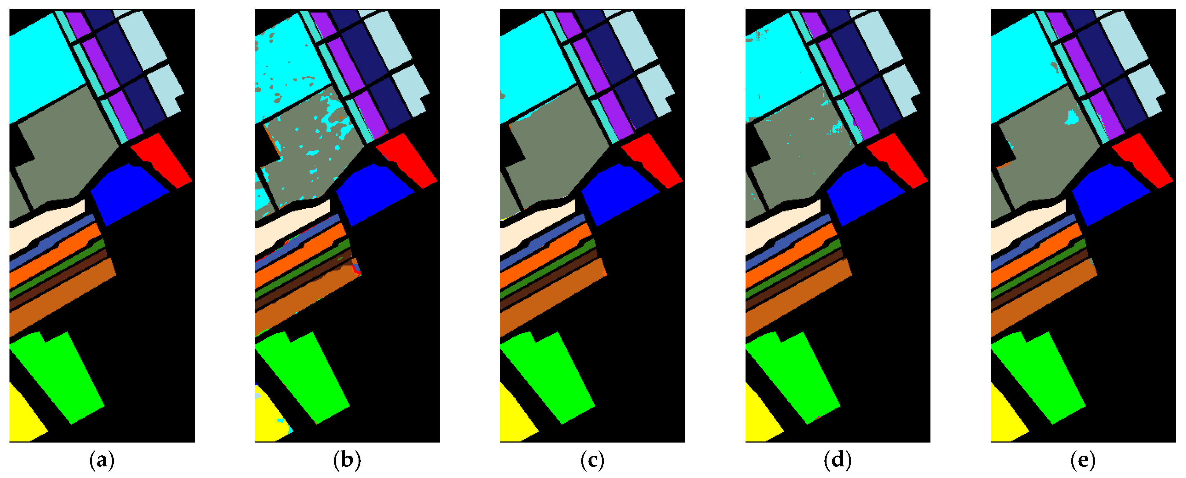
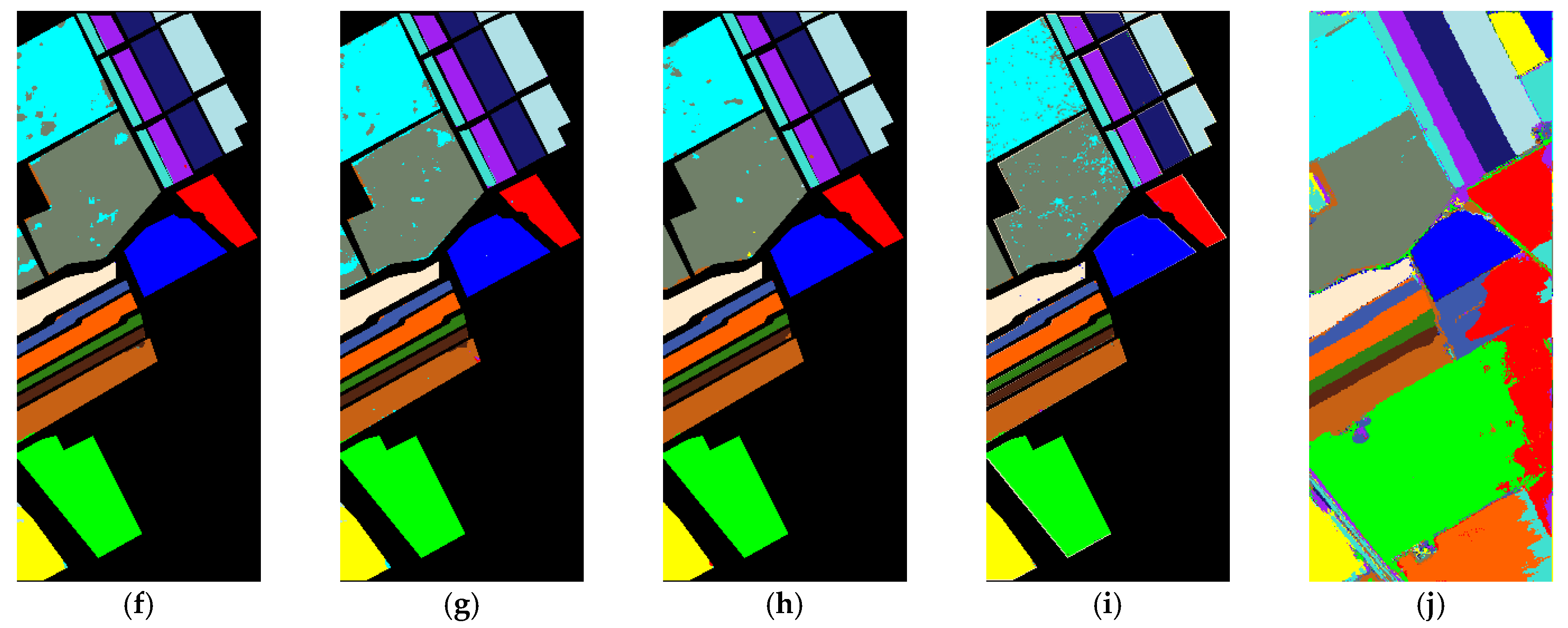
4.3. Experiment Results

This section compares the performance of the DSSFN model with a number of contemporary leading approaches, including SSRN [77], HSN [78], S3EResBOF [79], HSI-BERT [80], ASSMN [81], RSSAN [82], DAGCN [83], and SSFTT [84], all of which utilize open-source base code and find their optimal parameters in the relevant articles. After five rounds, the average results and standard deviations were recorded. The measure of algorithm performance is the metrics of the average results, and the standard deviation recorded in multiple experiments is used as a reference for robustness verification. The following is a brief introduction of these models.

(1) SSRN: The original 3D data cubes are input in the end-to-end network, and the spectral residual blocks and spatial residual blocks continuously learn the feature information in the hyperspectral images, connecting each 3D convolutional layer by residual block mapping.

(2) HSN: Using 3D convolution in the spectral dimension and 2D convolution in the spatial dimension. Compared to using only 3D convolution, hybrid convolutional networks lower the complexity of the network.

(3) S3EResBOF: A squeeze-and-excitation (SE) residual network for raw hyperspectral data feature extraction. To increase classification performance, each residual module is coupled with other 3D convolutional layers via an SE module.

(4) HSI-BERT: With a flexible input structure and strong generalization capability, global dependencies among pixels of hyperspectral data are represented via global perceptual fields. It is primarily composed of a multi-head attention process, in which various heads learn different feature information and encode the context in order to gain distinguishing traits.

(5) ASSMN: Utilize spectral feature extraction and spatial feature extraction networks to process hyperspectral data. On the spectrum side, Long Short Time Memory (LSTM) is employed to perceive multiscale spectral information. Using the convolutional LSTM (ConvLSTM) model, spatial contextual information that was previously disregarded is successfully extracted in the spatial sub-network.

(6) RSSAN: Utilizing the original 3D hyperspectral cube as input data, the features of spectral spatial feature learning are optimized by stressing the selection of important spectral bands for the classification and the suppression of worthless bands from the original input data.

(7) DAGCN: A framework convolutional network built on the deep attention graph is intended to extract deep abstract features and investigate the intrinsic correlations between HSI data by constantly changing the attention graph adjacency matrix to accommodate changes in each feature graph.

(8) SSFTT: The development of an information extraction module is accomplished by means of the integration of 3D and 2D convolution techniques. Furthermore, Gaussian-weighted feature markers are introduced to optimize the performance of the module. The resulting modified features are then employed in the training of the transformer module.

Comparison experiments are conducted on each dataset, and quantitative metrics and visualization results are provided for each method. The label of the dataset is denoted as (a), while the labeled pixel classification results of the comparison methods are represented as (b)–(i). The whole-image classification results of our method are indicated as (j). Figure 10, Figure 11, Figure 12 and Figure 13 show the classification maps obtained by different methods.

Table 1. Classification results of the proposed method and other leading methods on the IP dataset (%).

	SSRN	HSN	S3EResBOF	HSI-BERT	ASSMN	RSSAN	DAGAN	SSFTT	DSSFN
OA	94.16 ± 0.01	95.75 ± 2.87	97.02 ± 0.79	97.75 ± 0.00	98.30 ± 0.51	95.17 ± 0.76	96.86 ± 0.36	97.47	98.77 ± 0.26
AA	92.67 ± 0.01	92.56 ± 4.91	95.08 ± 2.59	90.13 ± 0.02	99.09 ± 0.36	92.54 ± 1.87	95.80 ± 0.87	96.57	97.76 ± 0.54
KAPPA	93.37 ± 0.06	95.17 ± 3.24	96.61 ± 0.91	97.43 ± 0.01	97.03 ± 0.59	94.49 ± 1.99	96.42 ± 0.41	97.11	98.81 ± 0.11
1	100	87.91	94.79	72.68	99.23	87.10	92.78	95.12	100
2	98.12	93.64	96.41	96.06	96.48	90.89	94.34	97.67	95.59
3	98.46	94.97	96.52	97.62	98.68	90.88	96.68	98.87	97.61
4	97.04	89.64	95.88	97.28	99.71	81.82	97.56	91.55	95.1
5	97.16	95.12	95.18	97.51	98.88	98.81	95.95	96.32	98.63
6	98.88	96.97	98.77	81.37	99.97	98.43	98.42	99.54	97.69
7	41.94	87.62	76.98	62.40	98.75	94.74	90.00	100	100
8	99.89	99.13	99.82	100	100	98.50	99.81	100	100
9	33.33	71.81	98.41	38.89	100	71.43	94.00	88.89	97
10	99.16	95.26	96.37	97.21	98.2	94.40	92.59	97.71	93.62
11	86.37	97.30	97.54	99.35	97.29	97.73	98.21	98.69	98
12	79.73	93.51	95.99	95.08	99.23	93.72	96.36	98.13	95.88
13	98.53	96.70	96.80	98.80	99.52	100	99.46	97.28	96.1
14	99.74	98.31	98.44	99.51	99.45	99.21	99.12	99.91	98.9
15	89.55	94.76	98.55	99.14	100	87.73	97.41	98.84	97.02
16	86.24	88.30	84.87	91.81	100	95.31	90.12	95.54	95.35

,

Table 2. Classification results of the proposed method and other leading methods on the KSC dataset (%).

	SSRN	HSN	S3EResBOF	HSI-BERT	ASSMN	RSSAN	DAGAN	SSFTT	DSSFN
OA	98.41 ± 0.02	96.52 ± 0.83	92.91 ± 5.12	97.69 ± 0.00	98.44 ± 0.45	93.04 ± 0.51	97.20 ± 0.57	93.82 ± 4.76	98.9 ± 0.23
AA	97.15 ± 0.02	94.40 ± 1.32	92.25 ± 4.05	95.89 ± 0.04	98 ± 0.36	90.33 ± 0.62	95.40 ± 0.17	89.60 ± 8.46	97.93 ± 1.01
KAPPA	98.23 ± 0.02	96.12 ± 0.93	92.11 ± 5.70	97.42 ± 0.01	98.27 ± 1.44	93.30 ± 1.71	96.89 ± 0.64	93.10 ± 5.38	98.7 ± 0.29
1	100	96.68	94.94	99.94	97.09	98.61	97.04	99.50	99.08
2	94.00	93.89	88.71	99.63	96.91	88.05	92.81	88.51	94.02
3	90.99	90.21	80.73	89.48	93.88	90.07	97.64	62.00	98.04
4	95.26	79.39	76.42	76.99	93.25	91.23	93.96	68.81	88.47
5	97.66	85.06	84.61	83.19	98.15	89.79	82.52	85.12	80
6	98.84	92.61	94.69	98.06	97.73	85,75	90.05	71.37	100
7	89.86	93.76	98.27	100	98.85	93.57	91.61	65.00	92.38
8	100	98.38	87.17	99.33	98.98	93.03	97.77	93.62	100
9	100	99.73	99.49	100	99.72	98.35	99.32	84.27	98.85
10	100	99.73	95.50	100	99.97	87.20	99.67	94.95	98.51
11	96.32	99.94	99.95	100	100	98.23	99.73	98.99	100
12	100	97.91	98.78	99.96	99.47	96.74	98.14	93.30	100
13	100	99.86	100	100	100	97.69	99.98	99.99	100

,

Table 3. Classification results of the proposed method and other leading methods on the PU dataset (%).

	SSRN	HSN	S3EResBOF	HSI-BERT	ASSMN	RSSAN	DAGAN	SSFTT	DSSFN
OA	99.52 ± 0.01	98.69 ± 1.40	97.68 ± 1.43	99.17 ± 0.00	96.26 ± 1.08	98.65 ± 0.31	99.44 ± 0.02	99.21	99.83 ± 0.02
AA	99.13 ± 0.01	98.36 ± 1.70	96.63 ± 1.80	99.79 ± 0.00	98.12 ± 0.32	97.93 ± 0.56	99.28 ± 0.02	98.69	99.26 ± 0.15
KAPPA	99.36 ± 0.02	98.24 ± 1.89	96.92 ± 1.88	99.05 ± 0.00	95.06 ± 1.4	98.22 ± 0.45	99.26 ± 0.02	99.15	99.78 ± 0.06
1	99.85	99.17	98.71	99.90	96.8	99.16	99.70	99.33	99.19
2	99.97	99.31	99.86	100	94.06	99.36	99.74	99.92	99.96
3	97.26	97.22	92.03	99.63	97.95	95.17	98.34	98.29	98.21
4	97.19	96.66	89.14	99.08	99.21	98.09	99.09	98.49	99.83
5	99.53	99.78	99.10	100	100	99.36	100	99.53	100
6	100	98.69	98.73	99.99	97.92	99.43	99.60	100	99.88
7	99.71	99.25	99.25	99.98	99.54	94.95	99.13	99.13	98.66
8	99.19	96.09	96.35	99.76	97.68	96.55	97.91	98.05	99.76
9	99.46	99.11	96.47	99.81	99.94	99.40	100	95.44	99.79

and

Table 4. Classification results of the proposed method and other leading methods on the SA dataset (%).

	SSRN	HSN	S3EResBOF	HSI-BERT	ASSMN	RSSAN	DAGAN	SSFTT	DSSFN
OA	96.62 ± 0.98	98.90 ± 1.60	98.37 ± 0.30	99.56 ± 0.089	98.44 ± 0.36	97.28 ± 2.42	99.04 ± 0.02	96.47 ± 0.56	99.67 ± 0.34
AA	98.49 ± 0.38	99.29 ± 1.04	99.16 ± 0.31	99.84 ± 0.022	99.36 ± 0.05	98.42 ± 1.11	99.39 ± 0.01	97.57 ± 0.35	99.36 ± 0.75
KAPPA	96.23 ± 1.08	98.77 ± 1.78	98.18 ± 0.70	99.42 ± 0.13	98.26 ± 0.26	96.97 ± 2.73	98.93 ± 0.02	96.07 ± 0.62	99.64 ± 0.28
1	100	99.99	99.93	100	100	99.98	100	99.92	99.95
2	99.98	99.93	100	100	100	99.69	100	99.99	99.97
3	100	99.95	99.97	100	99.89	99.72	100 ± 0.00	99.99	100
4	99.52	98.82	97.75	100	100	98.34	99.87	96.45	96.2
5	99.63	99.73	99.75	99.92	99.3	98.58	99.57	98.86	97.18
6	100	99.85	99.96	100	100	99.76	100	99.86	99.14
7	100	99.85	99.99	99.96	100	99.63	99.89	98.94	99.49
8	95.57	97.44	98.09	98.48	95.51	95.26	98.34	92.64	99.68
9	100	99.97	100	100	100	99.72	100	99.98	99.58
10	97.45	98.50	99.57	99.93	99.62	97.68	99.63	97.99	98.63
11	98.24	97.93	99.80	100	100	100.00	98.97	99.98	98.79
12	99.87	99.62	99.92	100	100	99.96	100	97.61	100
13	99.75	99.95	99.62	100	100	99.24	99.66	94.4	99.78
14	99.93	99.70	99.67	100	100	96.35	98.54	95.17	99.43
15	85.83	97.48	92.63	99.26	96.21	90.76	96.33	89.92	99.5
16	100	99.94	99.97	99.97	99.3	100.00	99.39	99.48	100

present the quantitative results (averaged over five experiments) of different methods.

In the first experimental scenario, the Indian Pines Scene is utilized to evaluate the performance of several classification techniques. 10% of the randomly selected ones are used as training samples, and the spatial dimension of the input data is 15 × 15. Comparing the experimental results of all models, the classification accuracy of classes 1, 7, and 9 deteriorates significantly. The overall number of samples for these three groups of data in the dataset is lower, as are the training samples. The better classification accuracy of the DSSFN classification method based on spectral and spatial patches demonstrates the advantages of combining spectral and spatial information. On the one hand, the self-attention mechanism is more advantageous than the attention-based classifier for the extraction of global information. It demonstrates that attention offers a solid foundation for deep learning networks and that mining the perceptual field significantly improves performance. On the other hand, raising the network’s depth confirms that the aggregation of multi-layer characteristics results in improved performance characterization. Overall, the classification results of DSSFN are superior to those of other evaluated networks, and there is a significant performance gain in comparison to the recently open-source SOTA hyperspectral classification, with a 3% and 2% improvement over HSN and SSTFF, respectively.

In the second experimental scenario, the training sample proportion of KSC is set as 15%, and the spatial dimension input data size is 15 × 15. Raising the size of patches can capture more peripheral information and enhance the classification accuracy, but at the expense of the training pace of the model; therefore, 15 × 15 is chosen after careful analysis. According to the classification results, the DSSFN model has the highest accuracy. Due to the rather sparse feature distribution of the KSC dataset, the OA of RSSAN and S3EResBOF is not particularly high. The KSC dataset exhibits a low level of label information, with only 10% of the pixel points containing labeled data. This issue arises from the neural network’s inability to extract profound features, resulting in the occurrence of local optima and overfitting. The utilization of the residual pyramid structure, which incorporates layer hopping connections, can enhance the capacity of the network to extract concealed features without necessitating an increase in the layer count. This, in turn, leads to an improvement in the overall efficiency of the network. This demonstrates that our proposed DSSFN network model has superior robustness in sparse data scenarios and outperforms other state-of-the-art methods.

The third experimental scenario is the dataset from the University of Pavia, with 5% randomly picked as the training set and a 15 × 15 data size. Considering that a large sliding window introduces excessive data smoothing problems. The classification results are depicted in Figure 11. The fused attention technique presented in this research is superior to HSI-BERT in its ability to reliably extract useful spatial location data and avoid the interference of wrong pixel points. The fully extracted spectral characteristics also play a significant role in enhancing the classification performance of the proposed approach in this research. For the IP and KSC datasets, our technique outperforms HSI-BERT, RSSAN, and DAGCN by 2%. However, there is no substantial improvement in the metrics OA, AA, and KAPPA on the PU dataset, mostly because the PU dataset has sufficient training samples for all methods to be trained evenly. This shows that our classification algorithm can produce more accurate results with less training data.

The final experimental scenario is the SA dataset, in which 10% of the labeled samples are selected as the training set and the other samples are used for validation. The input size is merely 11 × 11, and our proposed method earns the highest OA, AA, and KAPPA scores compared to all other methods. The next best approach is DAGCN, which is unable to accomplish deep feature extraction using attention networks employing 3D convolution and 2D convolution, as evidenced by the representation of the results. In the dataset, Class 8 is “Grap untrained” and Class 15 is “Vineyard untrained”. Based on the results of the visualization, it is evident that many of the methods in these two categories are highly perplexing due to the similarity of their feature characteristics. Due to the hyperspectral data, various features may exhibit the same spectral features and different spectral curves on the same features as a result of environmental influences, making it difficult to separate them without simultaneously deriving spatial and spectral features. In addition, the residual pyramid structure and self-attention mechanism employed in this research can expand the receptive field for target pixel classification.

4.4. Discussion of Validity

4.4.1. Discussion of the Efficiency of the Self-Attention

In order to determine the efficacy of the strategy for adding the self-attention module to the network, we conduct ablation experiments on all four datasets. M-att represents the spatial information flow with the addition of the self-attention module, whereas M-o represents the spatial information flow without the self-attention module. In the ablation experiments, all groups use the same training and test samples, and the OA, AA, and KAPPA on the IP dataset are +1.05%, +2%, and +1.19%, respectively; those on the PU dataset are +0.4%, +0.66%, and +0.53%, respectively; those on the SA dataset are + 0.88%, +0.43%, and +1.02%, respectively; and those on the KSC dataset were +0.43%, +0.27%, and +0.47%, respectively. The results demonstrate that utilizing the self-attention mechanism resulted in varying degrees of performance enhancement across all four datasets. Although adding the attention module increases the time of network iterations, the number of parameters, and the computation of the final model, it assists in refining the features and semantic content of the images, which is useful for hyperspectral image classification. The advantage of this strategy is that the self-attentive mechanism provides a better balance of accuracy and efficiency, which is difficult to achieve when optimizing the model for both accuracy and speed, as shown in

Table 5. Classification results of the proposed self-attention with four datasets (%).

	IP			PU			SA			KSC
	OA	AA	KAPPA	OA	AA	KAPPA	OA	AA	KAPPA	OA	AA	KAPPA
M-att	99.4	99.19	99.31	97.95	97.31	97.28	99.51	99.55	99.49	99.21	98.44	99.12
M-o	98.35	97.19	98.12	97.55	96.65	96.75	98.63	99.12	98.47	98.78	98.17	98.65

.

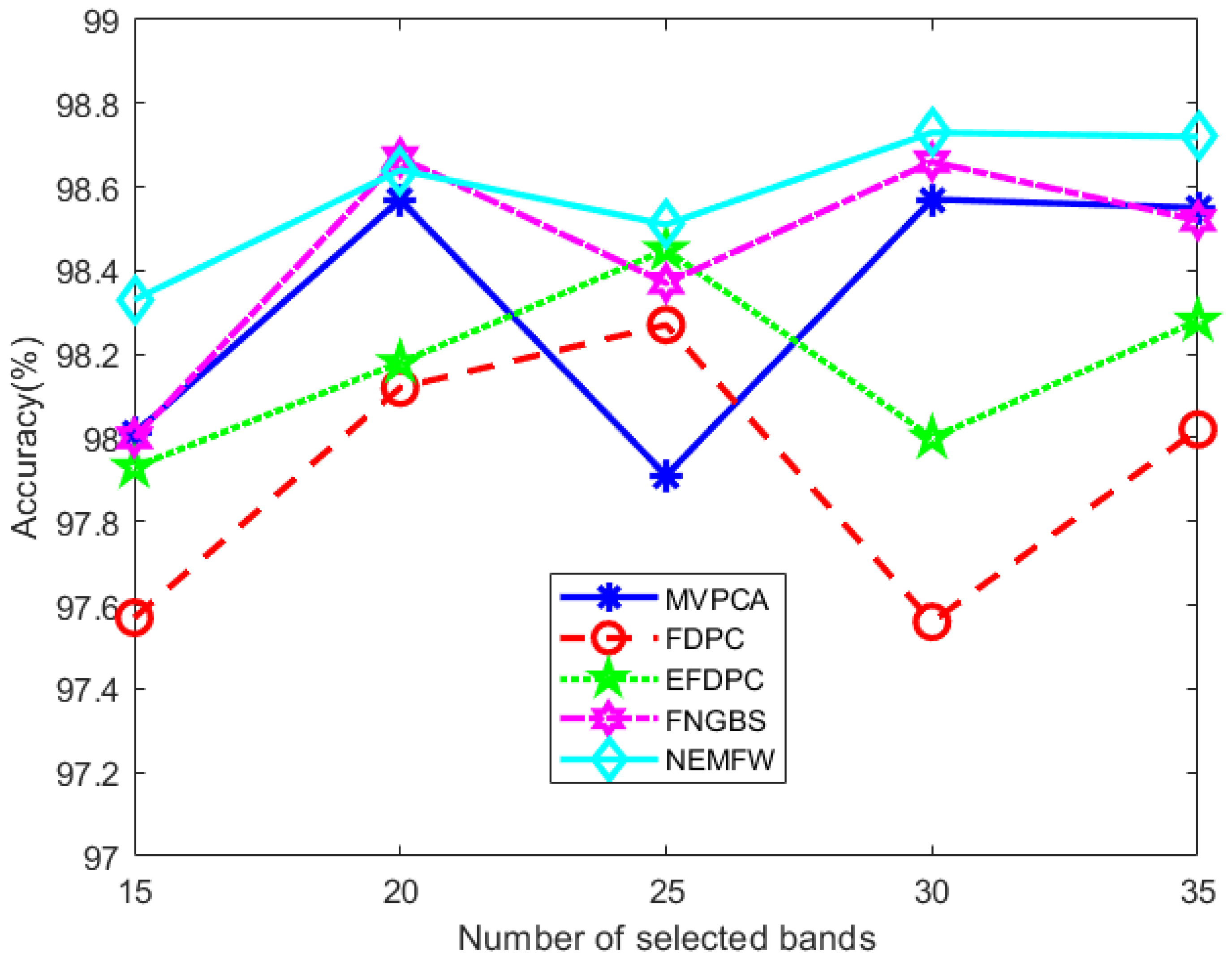
4.4.2. Discussion of the Validity of the Band Selection Method

The proposed sliding window grouping band selection method is contrasted and validated. The original IP dataset images, MVPCA downscaling [85], FDPC [86], EFDPC [55], and FNGBS [19] band selection methods, as well as the resulting [15,20,25,30,35] band images, are categorized accordingly. Moreover, a comparative analysis was conducted on the classification results generated by these models. Figure 14 illustrates the achieved classification outcomes.

MVPCA quantifies the difference of each band by ranking and selects the band with a higher ranking. The approach based on principal component analysis can focus the majority of the information on the first few principal component bands. However, the remainder of the principal components include a great deal of noise, and the selection of an excessive number of principal components might result in the introduction of noisy bands and an alteration of the classification findings. Methods for band selection incorporate sorting and clustering, such as FDPC and EFDPC. Nonetheless, when performing clustering processes, we typically consider spectra to be disordered, neglecting contextual information between bands. The subset of bands is determined by the local density and information entropy. However, the number of groupings must be predetermined, which is inapplicable to hyperspectral datasets with distinct bands. Additionally, the spatial structure information of each band is underutilized. As demonstrated previously, the correlation grouping-based SWGMF dimension reduction method described in this study can retrieve high-quality spectral information inside each band subgroup without introducing noise, hence providing efficient feature extraction from hyperspectral data.

4.4.3. Discussion of the Validity of Dual-Stream Networks

To further test the efficacy of the proposed new framework’s various branches and modules, we conducted comparative experiments while leaving the training set and other experimental parameters intact. There are three distinct models: SPE is the categorization of an image based on spectral data, SPA is the classification based on spatial data, and Fusion is the experimental outcome following information fusion.

Table 6. Classification results of the proposed dual-steam networks with four datasets (%).

	IP			PU			SA			KSC
	SPE	SPA	Fusion	SPE	SPA	Fusion	SPE	SPA	Fusion	SPE	SPA	Fusion
OA	82.63	97.56	98.77	95.33	99.82	99.83	92.87	99.8	99.82	83.86	98.73	98.9
MIOU	63.59	89.55	92.79	89.43	99.44	99.47	92.49	99.33	99.38	61.66	95.94	96.11
FWIOU	71.02	95.29	97.76	91.31	99.65	99.67	87.6	99.61	99.64	75.24	97.59	97.93
KAPPA	80.18	97.22	98.81	93.83	99.76	99.78	92.05	99.78	99.8	82.01	98.59	98.78

lists the outcomes of the comparative tests conducted on the four datasets. Relative to the individual information sources, the merged OA findings exhibit varying degrees of performance enhancement. The improvement is 16.14% and 1.21% on the IP dataset, 4.5% and 0.01% on the PU dataset, 6.95% and 0.02% on the SA dataset, and 15.04% and 0.17% on the KSC dataset, respectively. By 1D convolution, the emphasis is on spectral features, while through 2D convolution, the emphasis is on spatial features. The fused network can improve the network’s ability to learn discriminative features and achieve greater classification precision. Integrating the spatial-spectral network feature weights and capturing the interaction between features can boost the expression of fused features and improve the classification performance of hyperspectral images. The efficacy of the branch SPA, which is utilized for the extraction of spatial information, and the branch SPE, which is employed for the extraction of spectral information, exhibits variations across different datasets. This phenomenon may be attributed to gaps in the datasets resulting from variations in their collection methodologies. Moreover, in the context of the PU and SA datasets, the weighted fusion decision is enhanced by incorporating the feature extraction results from their corresponding branches. It is important to acknowledge that the precision of SPA is already significantly elevated, thereby limiting the possibility of additional improvement through fusion.

5. Conclusions

A dual-stream self-attention fusion network (DSSFN) for effective hyperspectral image classification with spatial and spectral fusion is proposed in this paper. On the basis of a sliding window grouped normalization matched filter for neighboring bands (SWGMF) band selection method, representative bands are selected to increase the extraction of effective information while minimizing redundancy across bands. The dual-stream network at once extracts information in spatial and spectral dimensions and classifies them after weighted fusion, which improves the capacity of the network to apply the extracted information with the data. The self-attention mechanism significantly captures hyperspectral image features at a distance through boosting the strength to study the correlation between the target pixels and the surrounding information. The residual structure in the pyramid structure mitigates the gradient vanishing problem and improves the ability to extract deep concealed features without increasing the network depth. As a consequence, the classification accuracy of the model is enhanced while its complexity is decreased. The proposed model is subjected to multiple experiments conducted on four publicly available datasets, all of which yield satisfactory classification results. A comparative analysis is then performed with some existing open-source methods, all of which exhibit substantial performance improvement. By demonstrating the potential of the self-attention mechanism in the Transformer structure, this paper provides a powerful tool for processing hyperspectral images, and future work will include further optimization of the network to combine CNN with Transformer for rapid and efficient feature extraction and image classification.

References

1. Zhang, M.; Li, W.; Du, Q. Diverse Region-Based CNN for Hyperspectral Image Classification. IEEE Trans. Image Process. 2018, 27, 2623–2634. [Google Scholar] [CrossRef] [PubMed]
2. Pearlman, J.S.; Barry, P.S.; Segal, C.C.; Shepanski, J.; Beiso, D.; Carman, S.L. Hyperion, a space-based imaging spectrometer. IEEE Trans. Geosci. Remote Sens. 2003, 41, 1160–1173. [Google Scholar] [CrossRef]
3. Jia, X.; Kuo, B.C.; Crawford, M.M. Feature Mining for Hyperspectral Image Classification. Proc. IEEE 2013, 101, 676–697. [Google Scholar] [CrossRef]
4. Benediktsson, J.A.; Palmason, J.A.; Sveinsson, J.R. Classification of hyperspectral data from urban areas based on extended morphological profiles. IEEE Trans. Geosci. Remote Sens. 2005, 43, 480–491. [Google Scholar] [CrossRef]
5. Wan, Y.; Hu, X.; Zhong, Y.; Ma, A.; Wei, L.; Zhang, L. Tailings Reservoir Disaster and Environmental Monitoring Using the UAV-ground Hyperspectral Joint Observation and Processing: A Case of Study in Xinjiang, the Belt and Road. In Proceedings of the IGARSS 2019–2019 IEEE International Geoscience and Remote Sensing Symposium, Yokohama, Japan, 28 July–2 August 2019; pp. 9713–9716. [Google Scholar]
6. Gevaert, C.M.; Suomalainen, J.; Tang, J.; Kooistra, L. Generation of Spectral–Temporal Response Surfaces by Combining Multispectral Satellite and Hyperspectral UAV Imagery for Precision Agriculture Applications. IEEE J. Sel. Top. Appl. Earth Obs. Remote Sens. 2015, 8, 3140–3146. [Google Scholar] [CrossRef]
7. Atkinson, J.T.; Ismail, R.; Robertson, M. Mapping Bugweed (Solanum mauritianum) Infestations in Pinus patula Plantations Using Hyperspectral Imagery and Support Vector Machines. IEEE J. Sel. Top. Appl. Earth Obs. Remote Sens. 2014, 7, 17–28. [Google Scholar] [CrossRef] [Green Version]
8. Grøtte, M.E.; Birkeland, R.; Honoré-Livermore, E.; Bakken, S.; Garrett, J.L.; Prentice, E.F.; Sigernes, F.; Orlandić, M.; Gravdahl, J.T.; Johansen, T.A. Ocean Color Hyperspectral Remote Sensing With High Resolution and Low Latency—The HYPSO-1 CubeSat Mission. IEEE Trans. Geosci. Remote Sens. 2022, 60, 1000619. [Google Scholar] [CrossRef]
9. Inoue, Y.; Dedieu, G.; Yoshida, N.; Saito, T.; Iwasaki, A.; Sakaiya, E. Assessing Crop Productivity in Decontaminated Farmland in Fukushima Using Micro-Satellite Venμs and Hyperspectral Sensing. In Proceedings of the IGARSS 2020–2020 IEEE International Geoscience and Remote Sensing Symposium, Waikoloa, HI, USA, 26 September–2 October 2020; pp. 5159–5162. [Google Scholar]
10. Tan, K.; Wu, F.; Du, Q.; Du, P.; Chen, Y. A Parallel Gaussian–Bernoulli Restricted Boltzmann Machine for Mining Area Classification With Hyperspectral Imagery. IEEE J. Sel. Top. Appl. Earth Obs. Remote Sens. 2019, 12, 627–636. [Google Scholar] [CrossRef]
11. Shimoni, M.; Haelterman, R.; Perneel, C. Hypersectral Imaging for Military and Security Applications: Combining Myriad Processing and Sensing Techniques. IEEE Geosci. Remote Sens. Mag. 2019, 7, 101–117. [Google Scholar] [CrossRef]
12. Sun, W.; Yang, G.; Du, B.; Zhang, L.; Zhang, L. A Sparse and Low-Rank Near-Isometric Linear Embedding Method for Feature Extraction in Hyperspectral Imagery Classification. IEEE Trans. Geosci. Remote Sens. 2017, 55, 4032–4046. [Google Scholar] [CrossRef]
13. Li, L.; Ge, H.; Gao, J.; Zhang, Y. Hyperspectral Image Feature Extraction Using Maclaurin Series Function Curve Fitting. Neural Process. Lett. 2019, 49, 357–374. [Google Scholar] [CrossRef]
14. Hong, D.; Yokoya, N.; Chanussot, J.; Xu, J.; Zhu, X.X. Joint and Progressive Subspace Analysis (JPSA) With Spatial–Spectral Manifold Alignment for Semisupervised Hyperspectral Dimensionality Reduction. IEEE Trans. Cybern. 2021, 51, 3602–3615. [Google Scholar] [CrossRef] [PubMed]
15. Hughes, G. On the mean accuracy of statistical pattern recognizers. IEEE Trans. Inf. Theory 1968, 14, 55–63. [Google Scholar] [CrossRef] [Green Version]
16. Rasti, B.; Hong, D.; Hang, R.; Ghamisi, P.; Kang, X.; Chanussot, J.; Benediktsson, J.A. Feature Extraction for Hyperspectral Imagery: The Evolution From Shallow to Deep: Overview and Toolbox. IEEE Geosci. Remote Sens. Mag. 2020, 8, 60–88. [Google Scholar] [CrossRef]
17. Sun, W.; Du, Q. Hyperspectral Band Selection: A Review. IEEE Geosci. Remote Sens. Mag. 2019, 7, 118–139. [Google Scholar] [CrossRef]
18. Sun, H.; Ren, J.; Zhao, H.; Sun, G.; Liao, W.; Fang, Z.; Zabalza, J. Adaptive Distance-Based Band Hierarchy (ADBH) for Effective Hyperspectral Band Selection. IEEE Trans. Cybern. 2022, 52, 215–227. [Google Scholar] [CrossRef] [PubMed] [Green Version]
19. Wang, Q.; Li, Q.; Li, X. A Fast Neighborhood Grouping Method for Hyperspectral Band Selection. IEEE Trans. Geosci. Remote Sens. 2021, 59, 5028–5039. [Google Scholar] [CrossRef]
20. Sawant, S.S.; Manoharan, P.; Loganathan, A. Band selection strategies for hyperspectral image classification based on machine learning and artificial intelligent techniques –Survey. Arab. J. Geosci. 2021, 14, 646. [Google Scholar] [CrossRef]
21. Zhang, R.; Ma, J. Feature selection for hyperspectral data based on recursive support vector machines. Int. J. Remote Sens. 2009, 30, 3669–3677. [Google Scholar] [CrossRef]
22. Guo, Y.; Cao, H.; Han, S.; Sun, Y.; Bai, Y. Spectral–Spatial HyperspectralImage Classification With K-Nearest Neighbor and Guided Filter. IEEE Access 2018, 6, 18582–18591. [Google Scholar] [CrossRef]
23. Chen, Y.; Lin, Z.; Zhao, X.; Wang, G.; Gu, Y. Deep learning-based classification of hyperspectral data. IEEE J. Sel. Top. Appl. Earth Obs. Remote Sens. 2014, 7, 2094–2107. [Google Scholar] [CrossRef]
24. Li, S.; Song, W.; Fang, L.; Chen, Y.; Ghamisi, P.; Benediktsson, J.A. Deep Learning for Hyperspectral Image Classification: An Overview. IEEE Trans. Geosci. Remote Sens. 2019, 57, 6690–6709. [Google Scholar] [CrossRef] [Green Version]
25. Hu, W.; Huang, Y.; Wei, L.; Zhang, F.; Li, H. Deep convolutional neural networks for hyperspectral image classification. J. Sens. 2015, 2015, 258619. [Google Scholar] [CrossRef] [Green Version]
26. Makantasis, K.; Karantzalos, K.; Doulamis, A.; Doulamis, N. Deep supervised learning for hyperspectral data classification through convolutional neural networks. In Proceedings of the 2015 IEEE International Geoscience and Remote Sensing Symposium (IGARSS), Milan, Italy, 26–31 July 2015; pp. 4959–4962. [Google Scholar]
27. Chen, Y.; Jiang, H.; Li, C.; Jia, X.; Ghamisi, P. Deep feature extraction and classification of hyperspectral images based on convolutional neural networks. IEEE Trans. Geosci. Remote Sens. 2016, 54, 6232–6251. [Google Scholar] [CrossRef] [Green Version]
28. He, L.; Li, J.; Liu, C.; Li, S. Recent Advances on Spectral–Spatial Hyperspectral Image Classification: An Overview and New Guidelines. IEEE Trans. Geosci. Remote Sens. 2018, 56, 1579–1597. [Google Scholar] [CrossRef]
29. Ahmad, M.; Shabbir, S.; Roy, S.K.; Hong, D.; Wu, X.; Yao, J.; Khan, A.M.; Mazzara, M.; Distefano, S.; Chanussot, J. Hyperspectral Image Classification—Traditional to Deep Models: A Survey for Future Prospects. IEEE J. Sel. Top. Appl. Earth Obs. Remote Sens. 2022, 15, 968–999. [Google Scholar] [CrossRef]
30. Zisserman, K.S.A. Two stream convolutional networks for action recognition in videos. In Advances in Neural Information Processing System; MIT Press: Cambridge, MA, USA, 2014; pp. 568–576. [Google Scholar]
31. Xue, Z.; Qian, S. Two-Stream Translating LSTM Network for Mangroves Mapping Using Sentinel-2 Multivariate Time Series. IEEE Trans. Geosci. Remote Sens. 2023, 61, 4401416. [Google Scholar] [CrossRef]
32. Wan, B.; Jiang, W.; Fang, Y.; Wen, W.; Liu, H. Dual-stream Self-attention Network for Image Captioning. In Proceedings of the 2022 IEEE International Conference on Visual Communications and Image Processing (VCIP), Suzhou, China, 13–16 December 2022; pp. 1–5. [Google Scholar]
33. Zhang, Y.; Huynh, C.P.; Ngan, K.N. Feature Fusion With Predictive Weighting for Spectral Image Classification and Segmentation. IEEE Trans. Geosci. Remote Sens. 2019, 57, 6792–6807. [Google Scholar] [CrossRef]
34. Hao, S.; Wang, W.; Ye, Y.; Nie, T.; Bruzzone, L. Two-Stream Deep Architecture for Hyperspectral Image Classification. IEEE Trans. Geosci. Remote Sens. 2018, 56, 2349–2361. [Google Scholar] [CrossRef]
35. Song, W.; Li, S.; Fang, L.; Lu, T. Hyperspectral Image Classification With Deep Feature Fusion Network. IEEE Trans. Geosci. Remote Sens. 2018, 56, 3173–3184. [Google Scholar] [CrossRef]
36. Cui, Y.; Li, W.; Chen, L.; Gao, S.; Wang, L. Double-Branch Local Context Feature Extraction Network for Hyperspectral Image Classification. IEEE Geosci. Remote Sens. Lett. 2022, 19, 6011005. [Google Scholar] [CrossRef]
37. Roy, S.K.; Manna, S.; Song, T.; Bruzzone, L. Attention-Based Adaptive Spectral–Spatial Kernel ResNet for Hyperspectral Image Classification. IEEE Trans. Geosci. Remote Sens. 2021, 59, 7831–7843. [Google Scholar] [CrossRef]
38. Li, N.; Wang, Z. Spectral-Spatial Fused Attention Network for Hyperspectral Image Classification. In Proceedings of the 2021 IEEE International Conference on Image Processing (ICIP), Anchorage, AK, USA, 19–22 September 2021; pp. 3832–3836. [Google Scholar]
39. Zhong, Z.; Li, Y.; Ma, L.; Li, J.; Zheng, W.-S. Spectral–Spatial Transformer Network for Hyperspectral Image Classification: A Factorized Architecture Search Framework. IEEE Trans. Geosci. Remote Sens. 2022, 60, 5514715. [Google Scholar] [CrossRef]
40. Xu, Y.; Du, B.; Zhang, L. Self-Attention Context Network: Addressing the Threat of Adversarial Attacks for Hyperspectral Image Classification. IEEE Trans. Image Process. 2021, 30, 8671–8685. [Google Scholar] [CrossRef]
41. Qing, Y.; Huang, Q.; Feng, L.; Qi, Y.; Liu, W. Multiscale Feature Fusion Network Incorporating 3D Self-Attention for Hyperspectral Image Classification. Remote Sensing 2022, 14, 742. [Google Scholar] [CrossRef]
42. Xia, J.; Cui, Y.; Li, W.; Wang, L.; Wang, C. Lightweight Self-Attention Residual Network for Hyperspectral Classification. IEEE Geosci. Remote Sens. Lett. 2022, 19, 6009305. [Google Scholar] [CrossRef]
43. Ghamisi, P.; Yokoya, N.; Li, J.; Liao, W.; Liu, S.; Plaza, J.; Rasti, B.; Plaza, A. Advances in Hyperspectral Image and Signal Processing: A Comprehensive Overview of the State of the Art. IEEE Geosci. Remote Sens. Mag. 2017, 5, 37–78. [Google Scholar] [CrossRef] [Green Version]
44. Liu, B.; Yu, X.; Zhang, P.; Yu, A.; Fu, Q.; Wei, X. Supervised deep feature extraction for hyperspectral image classification. IEEE Trans. Geosci. Remote Sens. 2017, 56, 1909–1921. [Google Scholar] [CrossRef]
45. Krizhevsky, A.; Sutskever, I.; Hinton, G.E. Imagenet classification with deep convolutional neural networks. Commun. ACM 2017, 60, 84–90. [Google Scholar] [CrossRef] [Green Version]
46. Li, Y.; Zhang, H.; Shen, Q. Spectral–spatial classification of hyperspectral imagery with 3D convolutional neural network. Remote Sens. 2017, 9, 67. [Google Scholar] [CrossRef] [Green Version]
47. Hamida, A.B.; Benoit, A.; Lambert, P.; Amar, C.B. 3-D Deep Learning Approach for Remote Sensing Image Classification. IEEE Trans. Geosci. Remote Sens. 2018, 56, 4420–4434. [Google Scholar] [CrossRef] [Green Version]
48. Conese, C.; Maselli, F.J.I.J.o.P.; Sensing, R. Selection of optimum bands from TM scenes through mutual information analysis. ISPRS J. Photogramm. Remote Sens. 1993, 48, 2–11. [Google Scholar] [CrossRef]
49. Stearns, S.; Wilson, B.; Peterson, J. Dimensionality Reduction by Optimal Band Selection for Pixel Classification of Hyperspectral Imagery; SPIE: Bellingham, WA, USA, 1993; Volume 2028. [Google Scholar]
50. Te-Ming, T.; Chin-Hsing, C.; Jiunn-Lin, W.; Chein, I.C. A fast two-stage classification method for high-dimensional remote sensing data. IEEE Trans. Geosci. Remote Sens. 1998, 36, 182–191. [Google Scholar] [CrossRef] [Green Version]
51. Yanfeng, G.; Ye, Z. Unsupervised subspace linear spectral mixture analysis for hyperspectral images. In Proceedings of the Proceedings 2003 International Conference on Image Processing (Cat. No.03CH37429), Barcelona, Spain, 14–17 September 2003; pp. 1–801. [Google Scholar]
52. Wang, Q.; Zhang, F.; Li, X. Optimal Clustering Framework for Hyperspectral Band Selection. IEEE Trans. Geosci. Remote Sens. 2018, 56, 5910–5922. [Google Scholar] [CrossRef] [Green Version]
53. Shahwani, H.; Bui, T.D.; Jeong, J.P.; Shin, J. A stable clustering algorithm based on affinity propagation for VANETs. In Proceedings of the 2017 19th International Conference on Advanced Communication Technology (ICACT), Pyeongchang, Republic of Korea, 19–22 February 2017; pp. 501–504. [Google Scholar]
54. Zeng, M.; Cai, Y.; Cai, Z.; Liu, X.; Hu, P.; Ku, J. Unsupervised Hyperspectral Image Band Selection Based on Deep Subspace Clustering. IEEE Geosci. Remote Sens. Lett. 2019, 16, 1889–1893. [Google Scholar] [CrossRef]
55. Jia, S.; Tang, G.; Zhu, J.; Li, Q. A Novel Ranking-Based Clustering Approach for Hyperspectral Band Selection. IEEE Trans. Geosci. Remote Sens. 2016, 54, 88–102. [Google Scholar] [CrossRef]
56. Xu, B.; Li, X.; Hou, W.; Wang, Y.; Wei, Y. A Similarity-Based Ranking Method for Hyperspectral Band Selection. IEEE Trans. Geosci. Remote Sens. 2021, 59, 9585–9599. [Google Scholar] [CrossRef]
57. Datta, A.; Ghosh, S.; Ghosh, A. Combination of Clustering and Ranking Techniques for Unsupervised Band Selection of Hyperspectral Images. IEEE J. Sel. Top. Appl. Earth Obs. Remote Sens. 2015, 8, 2814–2823. [Google Scholar] [CrossRef]
58. Yu, F.; Koltun, V. Multi-scale context aggregation by dilated convolutions. arXiv 2015, arXiv:1511.07122. [Google Scholar]
59. Vaswani, A.; Shazeer, N.; Parmar, N.; Uszkoreit, J.; Jones, L.; Gomez, A.N.; Kaiser, Ł.; Polosukhin, I. Attention is all you need. Adv. Neural Inf. Process. Syst. 2017, 30. [Google Scholar]
60. Hong, D.; Han, Z.; Yao, J.; Gao, L.; Zhang, B.; Plaza, A.; Chanussot, J. SpectralFormer: Rethinking Hyperspectral Image Classification With Transformers. IEEE Trans. Geosci. Remote Sens. 2022, 60, 5518615. [Google Scholar] [CrossRef]
61. Roy, S.K.; Deria, A.; Shah, C.; Haut, J.M.; Du, Q.; Plaza, A. Spectral–Spatial Morphological Attention Transformer for Hyperspectral Image Classification. IEEE Trans. Geosci. Remote Sens. 2023, 61, 5503615. [Google Scholar] [CrossRef]
62. Huang, L.; Chen, Y.; He, X. Spectral–Spatial Masked Transformer With Supervised and Contrastive Learning for Hyperspectral Image Classification. IEEE Trans. Geosci. Remote Sens. 2023, 61, 5508718. [Google Scholar] [CrossRef]
63. Dosovitskiy, A.; Beyer, L.; Kolesnikov, A.; Weissenborn, D.; Zhai, X.; Unterthiner, T.; Dehghani, M.; Minderer, M.; Heigold, G.; Gelly, S. An image is worth 16x16 words: Transformers for image recognition at scale. arXiv 2020, arXiv:2010.11929. [Google Scholar]
64. He, X.; Chen, Y.; Lin, Z. Spatial-Spectral Transformer for Hyperspectral Image Classification. Remote Sens. 2021, 13, 498. [Google Scholar] [CrossRef]
65. Qing, Y.; Liu, W.; Feng, L.; Gao, W. Improved Transformer Net for Hyperspectral Image Classification. Remote Sens. 2021, 13, 2216. [Google Scholar] [CrossRef]
66. Pan, X.; Ge, C.; Lu, R.; Song, S.; Chen, G.; Huang, Z.; Huang, G. On the Integration of Self-Attention and Convolution. In Proceedings of the 2022 IEEE/CVF Conference on Computer Vision and Pattern Recognition (CVPR), New Orleans, LA, USA, 18–24 June 2022; pp. 805–815. [Google Scholar]
67. He, K.; Zhang, X.; Ren, S.; Sun, J. Identity mappings in deep residual networks. In Proceedings of the Computer Vision–ECCV 2016: 14th European Conference, Amsterdam, The Netherlands, 11–14 October 2016; Part IV 14. pp. 630–645. [Google Scholar]
68. Szegedy, C.; Liu, W.; Jia, Y.; Sermanet, P.; Reed, S.; Anguelov, D.; Erhan, D.; Vanhoucke, V.; Rabinovich, A. Going deeper with convolutions. In Proceedings of the IEEE Conference on Computer Vision and Pattern Recognition, Boston, MA, USA, 7–12 June 2015; pp. 1–9. [Google Scholar]
69. Han, D.; Kim, J.; Kim, J. Deep pyramidal residual networks. In Proceedings of the IEEE conference on computer vision and pattern recognition, Honolulu, HI, USA, 21–26 July 2017; pp. 5927–5935. [Google Scholar]
70. Paoletti, M.E.; Haut, J.M.; Fernandez-Beltran, R.; Plaza, J.; Plaza, A.J.; Pla, F. Deep Pyramidal Residual Networks for Spectral–Spatial Hyperspectral Image Classification. IEEE Trans. Geosci. Remote Sens. 2019, 57, 740–754. [Google Scholar] [CrossRef]
71. Sergey, I.; Christian, S. Batch Normalization: Accelerating Deep Network Training by Reducing Internal Covariate Shift. In Proceedings of the 32nd International Conference on International Conference on Machine Learning, Lille, France, 6–11 July 2015; pp. 448–456. [Google Scholar]
72. Feichtenhofer, C.; Pinz, A.; Zisserman, A. Convolutional Two-Stream Network Fusion for Video Action Recognition. In Proceedings of the 2016 IEEE Conference on Computer Vision and Pattern Recognition (CVPR), Las Vegas, NV, USA, 27–30 June 2016; pp. 1933–1941. [Google Scholar]
73. Xu, Y.; Du, B.; Zhang, L. Beyond the Patchwise Classification: Spectral-Spatial Fully Convolutional Networks for Hyperspectral Image Classification. IEEE Trans. Big Data 2020, 6, 492–506. [Google Scholar] [CrossRef]
74. Green, R.O.; Eastwood, M.L.; Sarture, C.M.; Chrien, T.G.; Aronsson, M.; Chippendale, B.J.; Faust, J.A.; Pavri, B.E.; Chovit, C.J.; Solis, M. Imaging spectroscopy and the airborne visible/infrared imaging spectrometer (AVIRIS). Remote Sens. Environ. 1998, 65, 227–248. [Google Scholar] [CrossRef]
75. Kunkel, B.; Blechinger, F.; Lutz, R.; Doerffer, R.; Van der Piepen, H.; Schroder, M. ROSIS (Reflective Optics System Imaging Spectrometer)-A candidate instrument for polar platform missions. In Optoelectronic Technologies for Remote Sensing from Space; SPIE: Bellingham, WA, USA, 1988; pp. 134–141. [Google Scholar]
76. Cao, X.; Liu, Z.; Li, X.; Xiao, Q.; Feng, J.; Jiao, L. Nonoverlapped Sampling for Hyperspectral Imagery: Performance Evaluation and a Cotraining-Based Classification Strategy. IEEE Trans. Geosci. Remote Sens. 2022, 60, 5506314. [Google Scholar] [CrossRef]
77. Zhong, Z.; Li, J.; Luo, Z.; Chapman, M. Spectral–Spatial Residual Network for Hyperspectral Image Classification: A 3-D Deep Learning Framework. IEEE Trans. Geosci. Remote Sens. 2018, 56, 847–858. [Google Scholar] [CrossRef]
78. Roy, S.K.; Krishna, G.; Dubey, S.R.; Chaudhuri, B.B. HybridSN: Exploring 3-D–2-D CNN Feature Hierarchy for Hyperspectral Image Classification. IEEE Geosci. Remote Sens. Lett. 2020, 17, 277–281. [Google Scholar] [CrossRef] [Green Version]
79. Roy, S.K.; Chatterjee, S.; Bhattacharyya, S.; Chaudhuri, B.B.; Platoš, J. Lightweight Spectral–Spatial Squeeze-and- Excitation Residual Bag-of-Features Learning for Hyperspectral Classification. IEEE Trans. Geosci. Remote Sens. 2020, 58, 5277–5290. [Google Scholar] [CrossRef]
80. He, J.; Zhao, L.; Yang, H.; Zhang, M.; Li, W. HSI-BERT: Hyperspectral Image Classification Using the Bidirectional Encoder Representation From Transformers. IEEE Trans. Geosci. Remote Sens. 2020, 58, 165–178. [Google Scholar] [CrossRef]
81. Wang, D.; Du, B.; Zhang, L.; Xu, Y. Adaptive Spectral–Spatial Multiscale Contextual Feature Extraction for Hyperspectral Image Classification. IEEE Trans. Geosci. Remote Sens. 2021, 59, 2461–2477. [Google Scholar] [CrossRef]
82. Zhu, M.; Jiao, L.; Liu, F.; Yang, S.; Wang, J. Residual Spectral–Spatial Attention Network for Hyperspectral Image Classification. IEEE Trans. Geosci. Remote Sens. 2021, 59, 449–462. [Google Scholar] [CrossRef]
83. Bai, J.; Ding, B.; Xiao, Z.; Jiao, L.; Chen, H.; Regan, A.C. Hyperspectral Image Classification Based on Deep Attention Graph Convolutional Network. IEEE Trans. Geosci. Remote Sens. 2022, 60, 5504316. [Google Scholar] [CrossRef]
84. Sun, L.; Zhao, G.; Zheng, Y.; Wu, Z. Spectral–Spatial Feature Tokenization Transformer for Hyperspectral Image Classification. IEEE Trans. Geosci. Remote Sens. 2022, 60, 5522214. [Google Scholar] [CrossRef]
85. Chein, I.C.; Qian, D.; Tzu-Lung, S.; Althouse, M.L.G. A joint band prioritization and band-decorrelation approach to band selection for hyperspectral image classification. IEEE Trans. Geosci. Remote Sens. 1999, 37, 2631–2641. [Google Scholar] [CrossRef] [Green Version]
86. Rodriguez, A.; Laio, A. Clustering by fast search and find of density peaks. Science 2014, 344, 1492–1496. [Google Scholar] [CrossRef] [Green Version]
Figure 1. Hyperspectral data structure.
Remotesensing 15 03701 g001
Figure 2. 1D, 2D, 3D convolutions.
Remotesensing 15 03701 g002
Figure 3. Attention Mechanism.
Remotesensing 15 03701 g003
Figure 4. Schematic illustration of (a) basic residual units and (b) pyramid residual units.
Remotesensing 15 03701 g004
Figure 5. Overall Framework of DFFSN.
Remotesensing 15 03701 g005
Figure 6. Dimension Reduction Algorithm.
Remotesensing 15 03701 g006
Figure 7. Self-Attention Mechanism Process.
Remotesensing 15 03701 g007
Figure 8. Four hyperspectral image datasets with ground-truth maps. (a) Salinas Scene. (b) Pavia University. (c) Kennedy Space Center. (d) Indian Pines.
Remotesensing 15 03701 g008
Figure 9. OA results (%) of experiments with different parameter settings. (a) Learning Rate. (b) Spatial Patch Size. (c) Training Percent. (d) Convblock Depth.
Remotesensing 15 03701 g009aRemotesensing 15 03701 g009b
Figure 10. Classification maps for the IP with compared methods. (a) GroundTruth. (b) SSRN. (c) HSN. (d) S3EResBOF. (e) HSI-BERT. (f) ASSMN. (g) RSSAN. (h) DAGCN. (i) SSFTT. (j) DSSFN.
Remotesensing 15 03701 g010
Figure 11. Classification maps for the KSC with compared methods. (a) GroundTruth. (b) SSRN. (c) HSN. (d) S3EResBOF. (e) HSI-BERT. (f) ASSMN. (g) RSSAN. (h) DAGCN. (i) SSFTT. (j) DSSFN.
Remotesensing 15 03701 g011
Figure 12. Classification maps for the PU with compared methods. (a) GroundTruth. (b) SSRN. (c) HSN. (d) S3EResBOF. (e) HSI-BERT. (f) ASSMN. (g) RSSAN. (h) DAGCN. (i) SSFTT. (j) DSSFN.
Remotesensing 15 03701 g012
Figure 13. Classification maps for the SA with compared methods. (a) GroundTruth. (b) SSRN. (c) HSN. (d) S3EResBOF. (e) HSI-BERT. (f) ASSMN. (g) RSSAN. (h) DAGCN. (i) SSFTT. (j) DSSFN.
Remotesensing 15 03701 g013aRemotesensing 15 03701 g013b
Figure 14. OA results (%) of experiments with different band selection methods.
Remotesensing 15 03701 g014