Dual Homogeneous Patches-Based Band Selection Methodology for Hyperspectral Classification

Abstract

Homogeneous band- or pixel-based feature selection, which exploits the difference between spectral or spatial regions to select informative and low-redundant bands, has been extensively studied in classifying hyperspectral images (HSIs). Although many models have proven effective, they rarely simultaneously exploit homogeneous spatial and spectral information, which are beneficial to extract potential low-dimensional characteristics even under noise. Moreover, the employed vectorial transformation and unordered assumption destroy the implicit knowledge of HSIs. To solve these issues, a dual homogeneous pixel patches-based methodology termed PHSIMR was created for selecting the most representative, low-redundant, and informative bands, integrating hybrid superpixelwise adjacent band grouping and regional informative mutuality ranking algorithms. Specifically, the adjoining band grouping technique is designed to group adjacent bands into connected clusters with a small homogeneous pixel patch containing several homolabeled adjacent spatial points. Hence, the processing is efficient, and the superpixelwise adjoining band grouping can perceptually and quickly acquire connected band groups. Furthermore, the constructed graph and affiliated group avoid vectorial transformation and unordered assumption, protecting spectral and spatial contextual information. Then, the regional informative mutuality ranking algorithm is employed on another larger pixel patch within each homogeneous band group, acquiring the final representative, low-redundant, and informative band subset. Since the employed dual patches consist of homolabeled spatial pixels, PHSIMR is a supervised methodology. Comparative experiments on three benchmark HSIs were performed to demonstrate the efficiency and effectiveness of the proposed PHSIMR.

1. Introduction

There has been a growing interest in distinguishing disparate land-cover objects with available hyperspectral images (HSIs) recorded by special satellites [1,2,3]. Unlike traditional remote sensing imagery, HSI generally holds tens of thousands of sophisticated areal observations with hundreds of consecutive-wavelength spectral variables. It has been proven that abundant spectra and intensive scene pixels are beneficial to recognize different unmarked surfaces [4,5]. Despite the potential mentioned above, the attributes also have inevitably brought some obstacles to classifying HSIs, which include, but are not limited to the following: (1) the increments of band number and pixel size remarkably increase the time and cost of data processing and storage, and (2) the irreparable lacking of class labels and the huge spectral dimension quickly bring Hughes phenomenon, which significantly decreases the performance of classification or detection techniques [6,7].

It is known that reducing the number of recorded spectra is an effective solution to these issues [8,9]. In reality, since there exist amounts of redundancy, many highly correlative adjacent spectral variables may negatively influence the usefulness of global information [10]. Therefore, feature selection, i.e., band selection, is a helpful way to solve the mentioned problems by finding a band subset of meaningful details and low similarity to improve the analysis efficiency. Moreover, the band selection protects the input HSI’s original spatial information. It is conducive to further investigation, precisely the main reason that makes band selection outshine other dimension reduction methods [11,12].

Recently, many valid spectral band selection models have been presented, which can be seen as homogeneous [13,14,15] and global in manner [16,17,18,19,20,21], according to whether HSI is divided into disparate hybrid homogeneous groups. Among the global ways, several spectral bands are straightly acquired from the global information with specific metrics or strategies. However, since different homogeneous regions correspond to objects with distinct characteristics, globally measuring the informative scores of any bands is inappropriate [22,23]. Unfortunately, it may even be prevented from working when performing on vast HSI under limited facility conditions. According to the similarity among bands or pixels, homogeneous manners typically divide the whole spectral or spatial pixel set into different homogeneous groups, performing specific metrics or strategies within each group to acquire the final integrated band subset. The retained features are more irrelevant and less redundant, and the burden of data analysis is significantly reduced.

Generally speaking, homogeneous methodologies can be divided into nonadjacent [13,14,15] and adjacent manners [24,25,26,27,28,29,30,31,32,33,34]. The former tends to formulate band clusters with quantified similarities among any two variables, ignoring contextual information because of unordered assumptions [24]. Fortunately, the latter utilizes context to segment the entire HSI into connected homogeneous groups [24,25,26,27,28,29,30,31,32,33,34]. Recently, several novel adjacent manners have been presented and proven effective. Among these techniques, researchers usually establish a graph with a projection of spectral bands with a 2-D spatial structure to segment the pixel set into diverse homogeneous regions [28,29,30,31,32,33,34] or employ algebraic algorithms to divide the spectral set into neighboring groups [24,25,26,27]. For instance, to extract the contextual information of spectral bands, Wang et al. [24] developed a neighborhood band grouping mechanism to shrink the correlation evaluation to connected bands, which is conducive to protecting the main structure of highly related spectral variables. Identically, Zhang et al. [33,34] utilized graph representation to display spatial and spectral structural information, where nonadjacent bands are also considered irrelevant. Although these methods can group adjacent variables, they must be revised. Firstly, it should be noted that neither the 1-D algebraic algorithm nor the 2-D similarity graph of one dimension considers the structural information of the other dimension. Specifically, most similarity indexes, such as Euclidean distance [24], entropy [26,27,35], and l_2,1-norm [33,34], regard that the bands or pixels (the other dimension) are equally essential by assuming that the bands are independent or stretching the 2-D pixel matrix into a 1-D vector. Even the graph-based superpixel segmentation [31,32,33,34] is employed on a 2-D pixel matrix with a spectral transformation. The vectorial shift or unordered assumption leaves the central but implicit information out of consideration, including textual and geometric information conducive to classification.

After dividing, the adjacent manners usually adopt specific metrics to acquire the top influential bands within each group and then integrate them [24,25,26,27,28,29,30,31,32,33,34]. However, the weighting indexes have some issues. The metrics include two categories: individual metrics [36,37] and mutual metrics [38,39,40]. The former only considers each spectrum’s information, whereas the latter focuses on the relationship with other similar bands. These indexes either focus on the most quantified informative band of partial pixels or the most relevant band of each group, making it impossible to acquire representative and informative information simultaneously. Some models employed a combination of information and correlation qualifications to solve this problem [24,38]. Unfortunately, this type of algorithm may integrate conflicting indicators of disparate purposes, ignoring precise quantification of the significance of each component to the aggregative indexes. Furthermore, several adjacent band grouping models adopted a voting strategy [32] or iterative learning [33,34] within each group to search for proper subsets, which may bring more burdens of data processing.

Recently, due to the excellent generalization capability of distinguishing distinct spatial and spectral information in an underlying nonlinear structure, deep learning-based techniques have been increasingly applied in the classification of remote sensing images [41,42,43,44,45,46]. However, similar to existing nondeep learning models, most existing deep learning models rarely simultaneously exploit homogeneous spatial and spectral information, ignoring exploring the redundancy between the bands and the pixels simultaneously. Furthermore, these deep learning techniques overrely on the amounts of training samples and ask for sufficient internal storage, precisely opposite to our objectives of utilizing a small pixel patch to conduct band selection efficiently.

Above all, there are several open questions when it comes to the adjacent band- or pixel-based local feature selection:

• The data processing requires careful consideration and efficient utilization of original structural, morphological, or supplementary information. Specifically, when dealing with either pixels or bands, the other is usually turned into tractable vectors or mutually independent vertexes. As a result, the central but implicit features may be abandoned, bringing distorted estimation to some extent.
• For the score evaluation of each spectral band, the metrics need to consider the otherness of heterogeneous regions. Furthermore, the components of existing hybrid indexes may conflict when setting up particular metrics to obtain a subset.

To address the issues mentioned above, a novel feature selection methodology of dual homogeneous patches-based hybrid superpixelwise adjacent band grouping and informative mutuality ranking is created for hyperspectral classification, referred to as PHSIMR. The dominating contributions of the proposed framework are highlighted as follows.

• We design a hybrid superpixelwise adjacent band grouping on a homogeneous pixel patch to acquire similar and adjacent band groups, combing a finely designed algorithm to smooth boundary curves automatically. Instead of finding one component of hundreds of spectral features as the graph’s vertexes, our method retains complete and ordered contextual and morphological spectral and spatial information within the homogeneous spatial region. Moreover, the adopted pixel patch only contains several homolabeled adjacent spatial points so that the processing is efficient.
• The article also created a metric for band selection termed simplified informative mutuality, which can naturally measure each band’s influential score in the correlation degree with other homogeneous bands. Analogously, the proposed regional informative mutuality ranking algorithm is employed on homogeneous band groups and a pixel patch containing more homolabeled samples than the former utilized.
• Based on the employed homogeneous pixels and bands, the designed model is efficient, considers spatial and spectral contextual information, and can formulate representative, low-redundant, and informative band subsets. A series of comparative experiments on three benchmark HSIs demonstrates the efficiency and effectiveness of the proposed PHSIMR.

The remainder of this paper is organized as follows. Section 2 introduces the detailed descriptions of our band selection model, including homogeneous patch-based hybrid superpixelwise adjacent band grouping-based and homogeneous–multivariate patch-based informative mutuality. After that, a series of comparative experiments in Section 3 is conducted on three publicly available hyperspectral data sets. The discussion is given in Section 4. Finally, Section 5 presents the conclusion.

2. Proposed Methodology

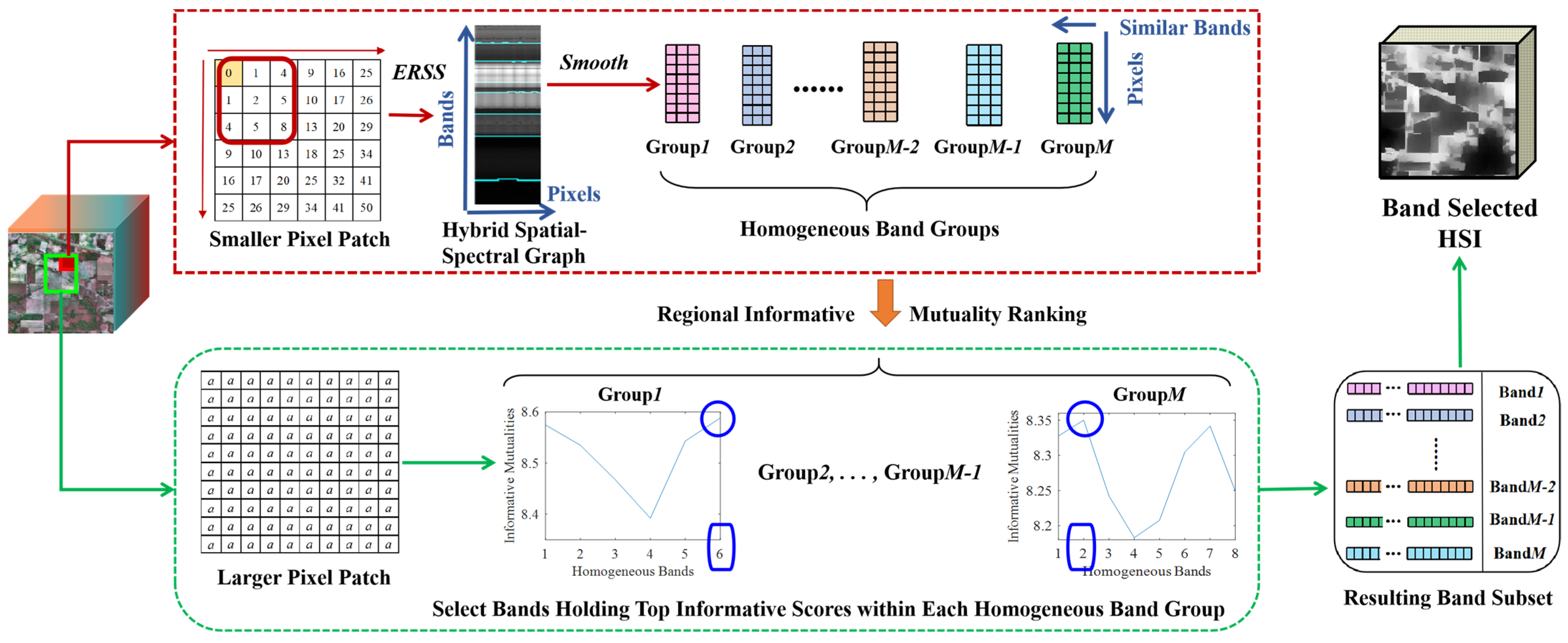
In this section, we expound on the proposed band selection module, whose flowchart is demonstrated in Figure 1.

First of all, the hybrid superpixelwise adjacent band grouping algorithm is conducted on a small homogeneous pixel patch. Specifically, we employed a small homogeneous pixel patch containing several neighboring homolabeled spatial pixels to construct a hybrid spatial–spectral graph, a 2-D grayscale image with all bands in rows and selected pixels in columns. Subsequently, the entropy rate superpixel segmentation (ERSS) [23] is performed on the 2-D grayscale image to acquire adjacent homogeneous band groups, combing with a finely designed algorithm to smooth boundary details automatically. Then, the developed regional informative mutuality ranking algorithm is exploited on a larger pixel patch to select the most representative, low-redundant, and informative bands holding top informative scores within each homogeneous band group. The second homogeneous pixel patch is more extensive than the former, and the dual homogeneous spatial patches are homolabeled.

2.1. Hybrid Superpixelwise Adjacent Band Grouping

For HSIs, it is known that adjacent homolabeled objects usually show similar spectral distributions among various bands. The particular affinity between geographic region and object category makes it possible to analyze HSI from a regional point of view [22]. Meanwhile, remarkable similarity exists among adjacent homogeneous spectral bands [24]. It is worth noting that the interference of noises is much smaller than the difference between heterogeneous features. Above all, since local adjacent pixels marked with the same class label are highly homogeneous, exploiting spectral contextual information from a homogeneous patch is feasible.

2.1.1. Construction of Hybrid Spatial–Spectral Graph

The input original HSI data cube can be represented as a three-order data cube $H\in {ℝ}^{W\times C\times B}$, in which W, C, and B represent the numbers of rows, columns, and bands of the original HSI, respectively. Before band grouping, we employ a local pixel patch containing homolabeled adjacent pixels to explore spectral bands’ geographic correlation. It is known that the distance of pixels in HSI represents the distance of the geographical locations in the actual scene [1]. Therefore, the closer the land-surface objects are, the more likely they are to exhibit similar properties. Inspired by this, a hybrid spatial–spectral band graph, $G_{B\times K}\in {ℝ}^{B\times K}$, is constructed, where each row represents one band vector within the spatial area of $K (K\ge 2)$ adjacent uniform pixels as:

$$G_{{}_{B\times K}}=\left(\begin{array}{cccc}{x}_{11}& x_{12}& \cdots & x_{1K}\\ x_{21}& x_{22}& \cdots & x_{2K}\\ ⋮& ⋮& \cdots & ⋮\\ x_{B1}& x_{B2}& \cdots & x_{BK}\end{array}\right)={(x_{ij})}_{B\times K}$$

(1)

where $x_{ij}$ is the jth observation of the ith spectrum vector, and K is the pixel length of the hybrid remodeling graph. Since the spectral dimension is fixed in rows, the hybrid spatial–spectral band graph $G_{B\times K}\in {ℝ}^{B\times K}$ mainly depends on the choice of K homogeneous pixels.

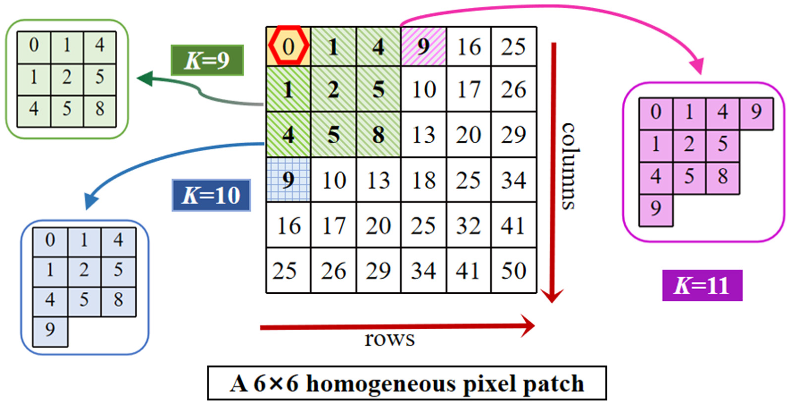
An ingenious strategy is designed to form actionable local pixel regions to obtain an optimal result, considering the consistency of pixel structure with natural structure. More precisely, we determine a local homogeneous pixel patch within a specific homolabeled area and experiment on the pixel patch according to the Euclidean square distance. After immobilizing a reference pixel, the Euclidean square distance is calculated to measure the distance from a geographically adjacent pixel to the fixed reference pixel. The distance map of 6 × 6 local pixels is shown in Figure 2, where each cell stands for one pixel, and the corresponding value is the distance to the initial spatial point located in the upper left corner of a testing patch, shown by the red regular hexagon.

As the sample region’s size rises, adding other samples to the pixel patch no longer decreases the overall distances to the reference sample. Hence, the selection strategy will help us find the optimal experimental patch as small as possible while validating the effectiveness of spatial homogeneity (found in the following subsection). In addition, local patch processing can significantly reduce the computational cost and exploit contextual characteristics to increase the performance of the band group.

2.1.2. Superpixelwise Adjacent Band Grouping

After hybrid graph construction, M connected homogeneous band regions can be generated by conducting ERSS [23] on $G_{B\times K}$ as follows:

$$G_{B\times K}(M)=\underset{k=1}{\overset{M}{\cup }}{\mathit{ħ}}_k \mathrm{s}.\mathrm{t} . {\mathit{ħ}}_i\cap {\mathit{ħ}}_j=\varnothing (i\ne j)$$

(2)

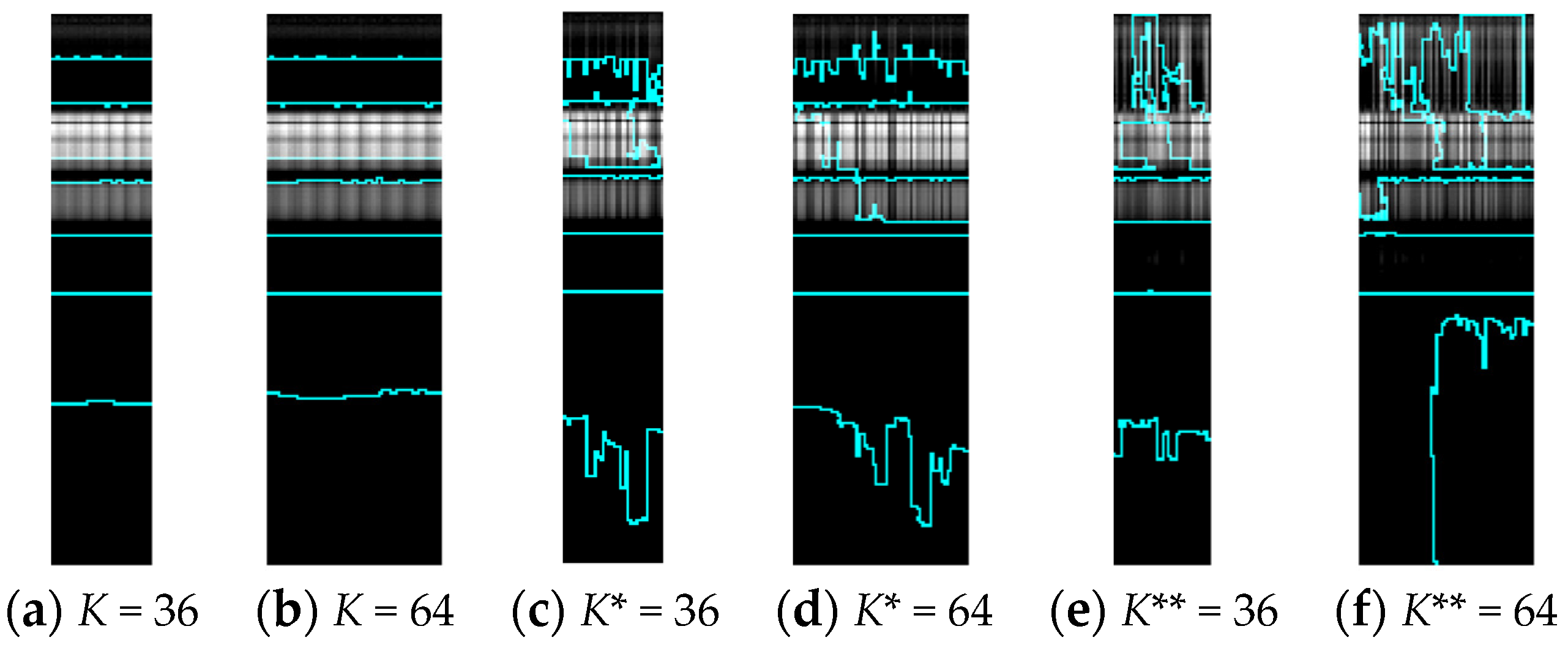
Here, $G_{B\times K}\left(M\right)$ represents the results by dividing the whole B bands into M connected clusters. The ERSS is steered on the spatial–spectral graph for generating level and smooth boundaries among heterogeneous bands. Instead of creating only one component by projecting spatial vectors or spectral variables [22], the proposed model retains the original spectral contextual features and primary texture information. Adjacent band grouping maps on the different experimental pixel regions in Indian Pines are demonstrated in Figure 3.

In Figure 3, K represents the number of pixels of the remodeling homogeneous hybrid graph, K* stands for the pixel size of the chart that holds randomly selected homolabeled pixels, and K** denotes the size of random pixels sampling from the global spatial set. The number of resulting band clusters W is fixed at 8, with boundary curves in green.

According to Figure 3, the performance of the proposed neighboring and local regional approach is superior to other sampling groups. Compared to (c)–(f), the borders of (a) and (b) are closer to the proposal we want to achieve, i.e., smooth and horizontal truncation to distinguish disparate spectral channels. The homogeneous pixel-patch methodology’s necessity, feasibility, and serviceability have been proven.

This strategy increases the averaging distance of selected pixels as the number of selected adjacent pixels rises. It is known that the spread of pixels in HSI represents the distance of the geographical locations in the actual scene. Therefore, the closer the land-surface objects are, the more likely they are to exhibit similar properties. Concretely, the overall similarity among the selected pixels increases as the testing region expands. Thus, we can easily find the minimum number of adjacent pixels to construct the 2-D grayscale image, obtaining more smooth heterogeneous band boundaries and reducing operating costs significantly. The superpixel-based band grouping method can not only regard the bands and pixels as variables and protect the original pixelwise value, but also set the stage for visualized neighboring band grouping with a 2-D variable graph rather than 1-D parallel spectral variables. Therefore, the complete and ordered contextual and morphological spectral and spatial information within the homogeneous spatial region are retained, significantly improving the effectiveness and efficiency of the proposed model by conducting a regional informative band selection on dual homogeneous pixel patches within each homogeneous band group.

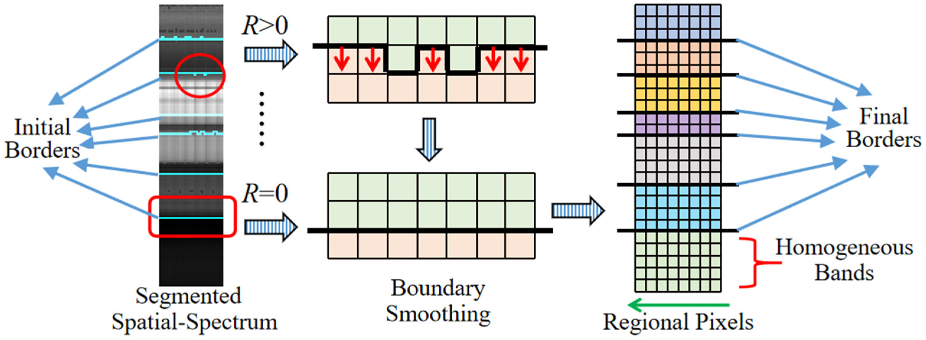
Although our approach is excellent, it is difficult to achieve faultless performance for the noticeable humps among the heterogeneous bands. There are two treated solutions to this issue: one is reducing the samples as much as possible; the other is manipulating a simple parallel shifting scheme. The latter can be achieved as follows. Assuming that one boundary is located in the nth band, the marker value v of the ith pixel $x_{nj}$ below the ultimate curve must meet the requirement of R = 0, where R is given by:

$$R={\displaystyle \sum _{j=1}^{K}v(x_{nj})} \mathrm{mod} K \mathrm{s}.\mathrm{t}. 2\le K\le 36$$

(3)

where the mod is adapted to return the residue R when the former number of the mod is divided by K. Since the parameter tuning region contains 6 × 6 pixels, the upper limit of K is fixed at 36. The bands are entirely separated by manually moving the nonhorizontal boundaries into a straight line along the band direction. In reality, the optimum size of the experimental region is almost always at most 16 invariably. The parallel shifting scheme is figuratively illustrated in Figure 4.

2.1.3. Model Optimization

The solution to the problem of how to acquire the optimal patch size is displayed in this part. To weigh the performance, a measure of confusion $E_n$ of the nth band of $G_{B\times K}(M)$ is adopted as follows:

$$E_n(K)=-{\displaystyle \sum _{t=1}^l\frac{c_{nt}}{K}{\log }_2(\frac{c_{nt}}{K})},t=1,\dots , l; {\displaystyle \sum _{t=1}^l{c}_{nt}}=K$$

(4)

where l is the number of indexes acquired by the ERSS on the nth row of $G_{B\times K}(M)$, and $c_{nt}$ denotes the length of index t developed by the ERSS. Perfect always results in the same index for each spectral row. Otherwise, l will surpass 1, so the confusion value is over 0. The confusion measure is also termed information entropy, which can reflect the confusion degrees of data distribution. Considering all rows of spectral bands, the global perplexity index is given by

$$E(K)={\displaystyle \sum _{n=1}^B{E}_n}(K),n=1, 2,\dots , B$$

(5)

The index $E(K)$ can explicitly measure the mass of the result on $G_{B\times K}(M)$ with K pixels. It is known that the less experimental confusion, the better the acquiring performance. Therefore, the treated way of obtaining the illustration is

$$\stackrel{}{\underset{K}{\mathrm{argmin}}} E\left(K\right) \mathrm{s}.\mathrm{t}. K=S,\dots ,36$$

(6)

Here, since the parameter tuning is on the local pixel region of 6 × 6, the upper limit of K is fixed at 36. On the strength that the satisfactory $E(K)=0$ will appear simultaneously with the same M and different K, S is set as the initial setup of the minimal patch size of K, significantly affecting the outcomes. In practice, different values of K result in various maps. Consequently, a threshold needs to be set for the parameter S. The specific setting of S is illustrated in the experiment section. Above all, the minimum column length that corresponded to the minimized $E(\cdot )$ is size of the final optimal experimental patch.

2.2. Informative Mutuality Ranking

After band grouping, we acquire M homogeneous connected band clusters, where adjacent spectral features have high intergroup variability and high intragroup correlation. A representative and low-redundant band subset can be set up by picking the most informative element within each group. A homogeneous pixel patch is adopted, similar to the aforementioned pixel patch for adjacent band grouping. The utilized patch is larger than the former one (i.e., $H\gg K$), but they both belong to a homolabeled region. Such operation reduces the running cost of band selection while avoiding the sampling uncertainty and unknown influence of other heterogeneous samples, which is proven effective via the experiment results.

Motivated by matrix-based Rényi’s α-order multivariate entropy function [47], we integrate the information weighting index into the above hybrid graph-based adjoining band grouping. Meanwhile, the measurement of informative importance on each intragroup spectral feature is also predigested because of its inherent nature. Specifically, a region that contains H adjacent homolabeled pixels can be reformulated as $G_{B\times H}$. Supposing that all bands have been partitioned into M homogeneous and balanced groups, the corresponding band subset ${\Gamma }_k$ of the kth group is formulated by

$${\Gamma }_k=\{{\mathit{\beta }}_k^1,{\mathit{\beta }}_k^2,\dots ,{\mathit{\beta }}_k^{{\varpi }_k}\}, \mathrm{s}.\mathrm{t}. \underset{k=1}{\overset{M}{\cup }}{\Gamma }_k={(G_{B\times H})}^T$$

(7)

where ${\varpi }_k$ is the length of the kth homogeneous group, and ${\mathit{\beta }}_k^{n_k}$($n_k$ = 1, 2, …,${\varpi }_k$) stands for the kth band vector of the set ${\Gamma }_k$. Actually, most of the set ${\Gamma }_k$ holds the same index k by the ERSS via Equation (2). Within any homogeneous band subset ${\Gamma }_k$(k = 1, 2, …, M), the locally informative mutuality $\Lambda ({\mathit{\beta }}_k^{n_k})$ of the band ${\mathit{\beta }}_k^{n_k}$ with other homoregional spectral bands ${\Gamma }_k\otimes {\mathit{\beta }}_k^{n_k}=\{{\mathit{\beta }}_k^1,\dots ,{\mathit{\beta }}_k^{n_k-1},{\mathit{\beta }}_k^{n_k+1},\dots ,{\mathit{\beta }}_k^{{\varpi }_k}\}$ can be generated by

$$\underset{}{\overset{}{\Lambda ({\mathit{\beta }}_k^{n_k})={\Phi }_{\alpha }({\mathit{\beta }}_k^{n_k})+{\Phi }_{\alpha }\left({\Gamma }_k\otimes {\mathit{\beta }}_k^{n_k}\right)-{\Phi }_{\alpha }\left({\Gamma }_k\right)}}$$

(8)

where ${\Phi }_{\alpha }({\mathit{\beta }}_k^{n_k})$ is the matrix-based Rényi’s α-order entropy function on ${\mathit{\beta }}_k^{n_k}$, which is a natural extension and generalization of the widely used Shannon’s entropy. The matrix-based Rényi’s α-order entropy can not only evaluate the entropy of the single variable (i.e., ${\Phi }_{\alpha }({\mathit{\beta }}_k^{n_k})$) or the multivariate joint entropy among multiple variables (i.e., ${\Phi }_{\alpha }({\mathit{\beta }}_k^{n_k})$), which can be formulated without probability density estimation as

$${\Phi }_{\alpha }({\mathit{\beta }}_k^{n_k})=S_{\alpha }({{\rm B}}_k^{n_k})=\frac{1}{1-\alpha }{\log }_2(tr{({{\rm B}}_k^{n_k})}^{\alpha }))$$

(9)

Here, tr denotes the trace function of the input square matrix, ${\Phi }_{\alpha }({\mathit{\beta }}_k^{n_k})=S_{\alpha }({{\rm B}}_k^{n_k})$, and ${{\rm B}}_k^{n_k}$ represents the normalized Gram matrices evaluated over the band ${\mathit{\beta }}_k^{n_k}$. By exploring the normalized positive definite square matrix over multiple spectral bands, the entropy can be directly calculated from the hyperspectral data without inaccurate probability density estimation over the high-dimensional data cube. Denoting C ◦ D the Hadamard product between the matrices C and D holding multiple spectral variables, the matrix-based multivariate joint Rényi’s α-order entropy of ${\Gamma }_k$ can be rewritten as:

$${\Phi }_{\alpha }\left({\Gamma }_k\right)=S_{\alpha }({{\rm B}}_k^1,{{\rm B}}_k^2,\dots ,{{\rm B}}_k^{{\varpi }_k})=S_{\alpha }\left(\frac{{{\rm B}}_k^1\circ {{\rm B}}_k^2\circ \cdots \circ {{\rm B}}_k^{{\varpi }_k}}{tr({{\rm B}}_k^1\circ {{\rm B}}_k^2\circ \cdots \circ {{\rm B}}_k^{{\varpi }_k})}\right)$$

(10)

where ${{\rm B}}_k^1$, ${{\rm B}}_k^2$, …, and ${{\rm B}}_k^{{\varpi }_k}$ are the normalized Gram matrices estimated over spectral bands ${\mathit{\beta }}_k^1$, ${\mathit{\beta }}_k^2$, …, and ${\mathit{\beta }}_k^{{\varpi }_k}$, respectively. The utilization of the Gram matrices ${{\rm B}}_k^1$, ${{\rm B}}_k^2$, …, and ${{\rm B}}_k^{{\varpi }_k}$ simplifies the calculation of the joint distribution to paired-element multiplication. Furthermore, based on the commutativity of the Hadamard product, the simplified multivariate patch-based informative mutuality $\tilde{\Lambda }({\mathit{\beta }}_k^{n_k})$ of ${\mathit{\beta }}_k^{n_k}$ can be defined as

$$\begin{array}{cc}\hfill \tilde{\Lambda }({\mathit{\beta }}_k^{n_k})=& {\Phi }_{\alpha }({\mathit{\beta }}_k^{n_k})+{\Phi }_{\alpha }\left({\Gamma }_k\otimes {\mathit{\beta }}_k^{n_k}\right)\hfill \\ \hfill =& S_{\alpha }({{\rm B}}_k^{n_k})+S_{\alpha }\left(\frac{{{\rm B}}_k^1\circ \cdots \circ {{\rm B}}_k^{n_k-1}\circ {{\rm B}}_k^{n_k+1}\cdots \circ {{\rm B}}_k^{{\varpi }_k}}{tr({{\rm B}}_k^1\circ \cdots \circ {{\rm B}}_k^{n_k-1}\circ {{\rm B}}_k^{n_k+1}\cdots \circ {{\rm B}}_k^{{\varpi }_k})}\right)\hfill \end{array}$$

(11)

It is worth noting that Equation (11) stands for the quantized informative score of the band ${\mathit{\beta }}_k^{n_k}$, and ${\Phi }_{\alpha }\left({\Gamma }_k\otimes {\mathit{\beta }}_k^{n_k}\right)$ denotes the quantized informative score of the rest. Since the total information ${\Phi }_{\alpha }\left({\Gamma }_k\right)$ is fixed, more significant remaining informative quantization will lead to larger informative mutuality. Moreover, more enormous rest information means a higher correlation of ${\mathit{\beta }}_k^{n_k}$ with other homogeneous bands. From this point, Equation (11) reflects the quantized information of each band’s influential score, i.e., the correlation degrees with other homogeneous bands. In other words, more considerable $\tilde{\Lambda }({\mathit{\beta }}_k^{n_k})$ means a higher correlation with other homogeneous bands.

Based on the homogeneity of each band group, the selected band has the highest correlation with other intragroup bands and low relation with other intergroup bands. Thus, the obtained band subset of representative, low-redundant, and informative is finally formulated as follows:

$$\{\underset{{\mathit{\beta }}_1^{n_1}}{\mathrm{argmax} }\tilde{\Lambda }({\mathit{\beta }}_1^{n_1}),\underset{{\mathit{\beta }}_2^{n_2}}{\mathrm{argmax} }\tilde{\Lambda }({\mathit{\beta }}_2^{n_2}),\dots ,\underset{{\mathit{\beta }}_M^{n_M}}{\mathrm{argmax} }\tilde{\Lambda }({\mathit{\beta }}_M^{n_M})\}$$

(12)

Unlike some typical band selection methods that evaluate the correlation between spectral variables and category labels, the band selection strategy in our article is narrowed into partial domains. Thus, the computing burdens and costs tomes can be remarkably reduced. With the local homogeneous spatial and spectral patches, we rank the evaluations of simplified informative mutuality according to the descending order and then find the top values within each spectral group.

2.3. Time Complexity Analysis

The computational complexity of the proposed PHSIMR in Algorithm 1 will be discussed as follows. P denotes the number of all spatial pixels, i.e., P = W × C. The main contribution to the complexity of the hybrid superpixelwise adjacent band grouping is the acquisition of ${{\displaystyle \cup }}_{k=1}^M {\mathit{ħ}}_k$, requiring the complexity of $\mathcal{O}$(BK × log(BK)). To calculate K, the time cost is $\mathcal{O}$(P). Besides, heterogeneous boundary smoothing is obtained by Equation (3), which takes $\mathcal{O}$(BK) to achieve Equation (7). The main contribution of the complexity of the homogeneous and multivariate patch-based informative mutuality is to rank the mutuality values within each band group via Equations (11) and (12). They take $\mathcal{O}$$(H^3{\varpi }_k{}^2)$ for the informative calculation within the kth homogeneous band group and $\mathcal{O}$(${\varpi }_k$) for ranking. Above all, the overall time complexity of MGSR is $\mathcal{O}$(BK × log(BK) + P + ${\displaystyle {\sum }_{k=1}^M{H}^3{\varpi }_k{}^2})$.

Algorithm 1 PHSIMR

Input:  Hyperspectral data set $H\in {ℝ}^{W\times C\times B}$, the number of selected bands M, the initial setup of homogeneous patch size for S, the patch size for information ranking H. Output:  The final spectral band subset. 1: Search for the optimal homogeneous patch size for K with S via Equation (6). 2: Establish a homogeneous hybrid spectral–spatial graph $G_{B\times K}\in {ℝ}^{B\times K}$. 3: Segment $G_{B\times K}\in {ℝ}^{B\times K}$ into ${{\displaystyle \cup }}_{k=1}^M {\mathit{ħ}}_k$ via Equation (2). 4: Smooth heterogeneous boundary to obtain homogeneous band groups ${\Gamma }_k=\{{\mathit{\beta }}_k^1,{\mathit{\beta }}_k^2,\dots ,{\mathit{\beta }}_k^{{\varpi }_k}\}$ via Equation (3). 5: Construct another homogeneous patch $G_{B\times H}\in {ℝ}^{B\times H}$. 6: Calculate simplified informative mutuality within each band group ${\Gamma }_k$ via Equation (11). 7: Rank the mutuality values within ${\Gamma }_k$ to find the top band $\underset{}{\mathrm{argmax} }\tilde{\Lambda }({\mathit{\beta }}_k^{n_k})$ via Equation (12). 8: Integrate all top bands into the final band subset.

3. Experiments and Analysis

In this section, we first briefly introduce three employed benchmark hyperspectral data sets. Then, the experiment’s procedure for classification setting, parameter tuning, and comparative approaches is presented. Finally, the comparison results on different remaining bands are displayed to verify the effectiveness and efficiency of the proposed algorithm.

3.1. Benchmark Data Sets

To demonstrate the performance of the proposed algorithm, we adopt three publicly available benchmark HSI data sets, which are Indian Pines, Salinas, and Botswana.

Table 1. Essential information on three benchmark HSIs.

Data Set	Spatial Size	Spectral	Class	Labeled Samples
Indian Pines	145 × 145	200	16	10,249
Salinas	512 × 217	204	16	54,129
Botswana	1476 × 256	145	14	3248

summarizes the critical information of each data set.

• Indian Pines: This data set was recorded by the airborne AVIRIS sensor over an Indian Pines test site. After removing 24 water-absorption spectral bands, there are 200 valid spectral bands within the wavelength range between 400 and 2500 nm, and the size of each band is 145 × 145 pixels. This image covers a mixed vegetation site divided into 16 land-cover classes [48].
• Salinas: The airborne AVIRIS sensor from the Salinas Valley test site also gathered this data set. After removing the bands of water absorption and noise, the image cube contains 204 spectral signatures within the wavelength range between 400 and 2500 nm with the size of 512 × 217 pixels. Additionally, the data set includes 16 types of different land covers.
• Botswana: This data set was acquired by the NASA EO-1 satellite sensor from Botswana. After removing several noisy bands, the test data cube contains 145 spectral signatures within the wavelength range between 400 and 2500 nm with a size of 1476 × 256 pixels. Additionally, the data set includes 14 classes of different land covers.

3.2. Experimental Procedure

3.2.1. Classification Setting

To measure the quality of the retained band subset, a widely used multiclass nonlinear classifier, a support vector machine (SVM) [49], is employed to evaluate the quality of the acquired band subset. The parameters of RBF kernel-based SVM are obtained by fivefold cross-validation. Moreover, 10% of labeled pixels of each class are randomly employed for training tasks on Indian Pines and Botswana, leaving the rest as the testing sets. Considering the vast amounts of labeled samples in Salinas, the size of the training sets is set as 1% per class to reduce execution costs. Except for parameter sensitivity experiments that operate SVM once, most experimental results are acquired by averaging the values from fivefold cross-validations to eliminate the effect of random operating that may bring errors. Moreover, for distinct approaches, the corresponding training set is identical for each validation.

Specifically, each algorithm is adopted on the input HSI to acquire the subset of original spectral features. After that, the SVM classifier is adopted to the resulting subset. After classification experiments, three well-known and convincing precision indexes are conducted to evaluate the capability of band selection for all methods, which are average accuracy (AA), overall accuracy (OA), and kappa coefficient (Kappa). Furthermore, the classification map using different colors for distinct classes can also demonstrate the classification results.

3.2.2. Comparison Methods

To validate the effectiveness of the proposed band selection algorithm, several novel band selection approaches are compared with the proposed model in different numbers of retained spectral features and different HSI data sets.

Several great local band selection methods are taken as matched groups to make parallel appraisals of the effectiveness of our model in different numbers of band subsets. Enhanced fast density-peak-based clustering (E_FDPC) [32] prioritizes the product values of local density and intracluster distance of each point within each cluster to form band subsets. Optimal clustering framework (OCF) [15] presents an optimal clustering framework and a ranking on clusters strategy to obtain the optimal result for a particular form of objective function under a reasonable constraint. According to our entropy-based model and E_FDPC mentioned above, we adopt the entropy-E_FDPC type of OCF to conduct comparisons. Fast neighborhood grouping band selection (FNGBS) [24] devises a novel refined band partition strategy and chooses representative bands with local density and partial information entropy. The graph-regularized spatial–spectral subspace clustering method (GRSC) [31] selects top representative bands by combining a self-representation subspace clustering model with a region-aware similarity graph. Robust dual graph self-representation (RDGSR) [34] uses ERSS on the input data’s first principal component to extract spatial and spectral information and learns the optimal coefficient matrix to obtain the ideal band subset. It is worth noting that E_FDPC and OCF are clustering-based band selection methods, whereas others are grouping-based band selection models.

We gathered and tested the corresponding code of each compared method with parameters set similarly to the suggested values. In addition, a method that takes all spectral bands (All_Bands) as the input of the experimental classifier also serves as one of the control groups. We gathered and tested the corresponding code of each compared method with parameters set the same as the suggested values as much as possible. Among these competitors and the proposed method, since the number of retained bands is an unknown key parameter to each model, the sizes of the experimental subset are set within the range from 5 to 50.

3.3. Model Study

3.3.1. Parameter Tuning

Two hyperparameters must be tuned in advance with a grid-search strategy, i.e., the number S in Equation (6) of adjacent samples when operating spatial–spectral adjacent band grouping and the size H in Equation (7) of the homogeneous region when calculating patch-based informative mutuality. Parameter S is formulated for self-established spatial–spectral grayscale images to produce homogeneous and no-overlap regions of the spectral band. H is used to pick the final band within each resulting homogeneous region. Since these two fundamental parameters are chosen from the same part of only one label, we try to find the ideal experimental area before analyzing the impacts of these two essential parameters.

The ideal experimental area should cater to the following factors, which are (1) sufficient pixels and (2) low noise interference. The former can be easily observed from the input data, but the latter needs band grouping experiments until the heterogeneous group boundary approximates a straight line. To this end, we experiment on each data set with each category, finding that the optimal experimental areas of Indian Pines, Salinas, and Botswana are Grass-pasture, Grapes-untrained, and the 8th class, respectively; this no longer describes the corresponding specific experimental results because of space cause. In a word, the two parameters above are tuned within these areas. Considering the computational time and different amounts of labeled samples, the number of homogeneous pixels H is set to 100, 200, 300, and 400 when using Indian Pines and Salinas (or 50, 100, 150, and 200 for Botswana), respectively. The initial manipulative value S for band grouping covers the integers from 2 to 4.

It should be noted that the classification accuracy usually rises as the number of bands rises, until the dimension arrives at a specific big integer. Such a phenomenon may result from the obtained boundaries of heterogeneous band regions that need to be more precise or attributed to the features on homogeneous pixels being too similar to be distinguished. Fortunately, although no setting can be optimal for all dimensions, the proposed band selection method can easily acquire satisfying performance.

Table 2. Classification results in OA (%) with different parameter sets and dimensions on Indian Pines.

S	H	5	10	15	20	25	30	35	37	40	42
2	100	71.03	75.85	78.15	78.43	79.08	81.42	79.38	80.40	81.70	80.41
	200	72.84	77.21	78.46	77.41	78.39	81.35	81.32	81.25	82.02	79.12
	300	72.21	76.87	79.78	79.82	80.90	81.79	82.28	82.31	82.62	80.32
	400	73.37	78.02	79.07	80.44	81.34	81.64	82.11	82.69	82.36	79.13
3	100	71.03	78.85	78.99	80.42	79.08	81.42	80.49	80.40	79.19	78.22
	200	72.84	78.64	78.99	80.30	78.39	81.35	80.87	81.25	78.46	78.29
	300	72.21	80.11	80.58	81.80	80.90	81.79	81.71	82.31	79.89	79.00
	400	73.37	79.63	79.20	80.96	81.34	81.64	81.85	82.69	79.52	77.55
4	100	71.03	78.85	78.99	78.94	79.08	81.42	79.38	80.40	79.19	78.22
	200	72.84	78.64	78.99	79.16	78.39	81.35	81.32	81.25	78.46	78.29
	300	72.21	80.11	80.58	80.35	80.90	81.79	82.28	82.31	79.89	79.00
	400	73.37	79.63	79.20	80.47	81.34	81.64	82.11	82.69	79.52	77.55

shows the classification results of Indian Pines on different parameter settings. One can observe that the influence of parameter H is more significant than parameter S. Moreover, the results obtained by S = 2 and S = 3 are similar. Based on the results, the parameters S and H are set to 2 and 300, respectively. The classification results of parameter sensitivity experiments on Salinas and Botswana are depicted in

Table 3. Classification results in OA (%) with different parameter sets and dimensions on Salinas.

S	H	5	10	15	20	25	30	35	37	40	42
2	100	89.82	89.76	91.42	91.09	91.72	91.70	91.46	91.68	91.42	90.97
	200	89.44	90.27	91.57	91.49	91.79	91.76	91.71	91.56	91.45	91.04
	300	89.60	90.57	91.10	91.62	91.70	91.38	91.70	91.50	91.50	90.92
	400	89.50	90.31	90.93	91.42	91.65	91.94	91.93	91.76	91.56	90.99
3	100	89.82	90.12	91.42	91.09	91.40	91.50	91.23	91.47	90.95	90.97
	200	89.44	90.20	91.57	91.49	91.65	91.63	91.75	91.35	91.04	91.04
	300	89.60	90.62	91.10	91.62	91.58	91.78	91.61	91.39	90.94	90.92
	400	89.60	90.61	90.97	91.63	91.26	91.79	91.82	91.36	91.01	90.87
4	100	89.82	91.16	91.42	91.09	91.30	91.50	91.23	91.47	90.95	90.97
	200	89.44	90.92	91.57	91.49	91.64	91.63	91.75	91.35	91.04	91.04
	300	89.60	91.15	91.10	91.62	91.56	91.78	91.61	91.39	90.94	90.92
	400	89.60	90.82	90.97	91.63	91.51	91.79	91.82	91.36	91.01	90.87

and

Table 4. Classification results in OA (%) with different parameter sets and dimensions in Botswana.

S	H	5	10	15	20	25	30	35	37	40	42
2	50	85.94	90.26	90.44	90.95	90.64	90.13	91.33	89.78	90.88	91.12
	100	85.91	90.26	90.81	90.33	89.72	89.13	90.85	90.33	90.50	90.44
	150	86.15	88.82	88.93	90.26	89.54	89.58	90.54	90.47	90.37	91.12
	200	86.66	88.79	88.52	90.50	89.92	90.06	90.54	90.23	90.02	91.22
3	50	85.94	90.26	89.99	90.78	90.57	90.61	90.30	90.95	91.36	91.12
	100	85.91	90.26	90.20	89.85	90.61	90.40	89.99	90.64	91.16	91.36
	150	86.15	88.82	89.00	89.78	90.81	89.65	89.89	90.26	90.88	90.78
	200	86.66	88.79	89.17	89.85	90.71	90.26	90.88	90.95	91.70	91.33
4	50	85.94	90.26	89.99	90.57	90.57	90.61	91.05	90.95	91.36	91.12
	100	85.91	90.26	90.20	90.06	90.61	90.40	90.98	90.64	91.16	91.36
	150	86.15	88.82	89.00	89.99	90.81	89.65	90.57	90.26	90.88	90.78
	200	86.66	88.79	89.17	88.79	90.71	90.26	91.40	90.95	91.70	91.33

, respectively. Similarly, the parameter settings are such that S = 2 & H = 400 and S = 4 & H = 50 are empirically set as the fixed values for Salinas and Botswana, respectively.

3.3.2. Ablation Study

The proposed band selection algorithm consists of two main phases: dividing the input bands into distinct homogeneous groups in a spatial–spectral manner and picking the most informatively representative band within each group using local adjacent pixels.

To validate the effectiveness of each component, we utilize a classic divide-and-conquer strategy to conduct an ablation study. Specifically, to illustrate the effectiveness of adjacent band grouping, the proposed homogeneous and multivariate patch-based informative mutuality (HMIM) and partial information entropy (PIE) are employed as control groups without band grouping. HMIM is a comparative method that picks the most informatively representative band by the same mutual information index as our model without processing to segment bands. PIE is a simplified variant of HMIM, evaluating the importance of each spectral band by randomly selected samples. PIE aims to rank Shannon’s entropy values of all bands in descending order to acquire an optimal subset.

To verify the effectiveness of the proposed band-picking index, HS-PIE (hybrid superpixelwise adjacent band grouping with PIE) is introduced, which employs the aforementioned partial information entropy after the proposed band grouping algorithm. HS-RIM (HS and random pixel-based informative mutuality) is also adopted on random pixels, utilizing the proposed band-picking index without homogeneous processing. In addition, the results of our model and all bands are demonstrated. The classification results for different components and different numbers of bands are shown in Figure 5.

One can observe that the proposed band selection algorithm is superior to other algorithms in most cases, in that it acquires excellent accuracy across different data sets and dimensions. On the one hand, the classification results of HMIM and PIE are markedly lower than other band grouping-based models. It reveals that the proposed adjacent band grouping method can effectively increase the representation of remaining bands, thus increasing classification performance. On the other hand, the measure proposed in this study is also superior to other band grouping-based methods, entropy-based models, and all bands. Concerning HS-PIE, the proposed band-picking index can result in more representative and informative bands that help for further investigation. The effectiveness of the homogeneous operating region is also demonstrated by comparing HS-RIM with our model. In conclusion, all our model’s components are practical and significantly improve the classification performance.

3.4. Comparison Results

3.4.1. Effectiveness Study

To validate the effectiveness of PHSIMR, we conducted experiments to select different sizes of spectral subsets by distinct local band selection models and evaluate the performance of the results with the adopted SVM classifier. The averaged OA curves of all listed algorithms and different band numbers on three benchmark hyperspectral data sets are presented in Figure 6. It should be noted that the reason why the results of RDGSR are not shown in Figure 6b is that the PC is prone to be out of memory when we conduct RDGSR on Salinas.

Before further analysis, we mainly focus on the OA curves in Figure 6 to obtain the optimal number of recommended bands. One can decide the size of the adopted subset from two aspects. One is the absolute magnitude of accuracy, which means we must compare the OA values of PHSIMR in different band numbers. Another is relative accuracy, which compares our accuracy and the values corresponding to other comparative models. Specifically, the proposed PHSIMR outperforms competitors according to OA curves and classification maps in general. From the curves of the remaining algorithms, one can find that it is difficult to exceed the entire spectral bands. Likewise, the accuracy of the proposed model can surpass it with some settings, which can be attributed to the precise adoption of informative and representative spectra subsets. PHSIMR considers the contextual information of both spectral and spatial dimensions, thereby reducing the redundancy and improving the quality of the band set.

Actually, the decision of the band number makes reference to the recommended number of bands algorithm in [24], which aims to find the minimum number of recommended bands by determining the inflection point of the discrete probability curve of different numbers of selected spectral bands. However, the algorithm in [24] defines the recommended number of bands from the point of lowering the redundancy of remaining bands as much as possible rather than enhancing the representative and informative characteristics to promote classification accuracy. Therefore, the classification results obtained by the recommended bands rarely meet the need for classification to recognize unlabeled spatial pixelwise objects. Furthermore, the performances of all methods tend to become higher as the subset size becomes larger, mainly attributed to the more discriminant features the subset offers. For all HSIs, the advantages of PHSIMR are apparent once the band numbers exceed a specific number. To this end, we integrated the recommended number of bands algorithm in [24] with practical classification accuracy values in OA, finding the final size of chosen band subset closer to both the minimum number of recommended bands and the actual classification performance. Figure 7 provides the discrete probabilities acquired by the algorithm in [24] of different band subsets on the employed three HSI data sets, where the minimum number of bands is shown by the red dot.

However, according to the OA curves of different numbers of remaining bands in Figure 7, we can find that the resulting OA values obtained by the recommended bands rarely meet the need for satisfactory classification performance. To acquire the desired results, we try to find an acceptable band subset that significantly outperforms comparisons and holds as few bands as possible. Considering that more bands bring more computing costs, the numbers of recommended bands are fixed at 18, 22, and 18 for Indian Pines, Salinas, and Botswana, respectively. For each local band selection algorithm, the distributions of selected bands of different models and data sets are displayed in Figure 8.

Since remarkable correlations exist among adjacent bands, it is feasible to evaluate the redundancy degrees of selected band sets according to the distribution shapes. From the distributions plotted in Figure 8, the resulting subsets obtained by our method are dispersed and robust to different HSIs. Unlike PHSIMR, the spectral subsets of E-FDPC, GRSC, and RDGSR demonstrate aggregation characteristics, especially on Indian Pines and Botswana. However, redundancy is not the sole criterion for testing the truth. When combined with corresponding classification performance, we can more objectively evaluate the quality of obtained bands. Although OCF and FNGBS can also select dispersed subsets, the results could be more representative according to the OA curves in Figure 6. Above all, our algorithm can produce both low-redundant and representative band subsets.

In addition, the classification results are wholly given with the classification accuracy values in

Table 5. Classification accuracy values (%) followed by corresponding standard errors.

Data Set	Index	E_FDPC [32]	OCF [15]	FNGBS [24]	GRSC [31]	RDGSR [34]	PHSIMR
Indian Pines	OA	69.57 ± 0.71	79.65 ± 1.51	78.49 ± 1.05	79.55 ± 1.02	68.21 ± 0.97	82.85 ± 0.55
	AA	70.00 ± 2.31	78.36 ± 1.47	78.17 ± 1.45	75.49 ± 0.89	66.50 ± 3.18	82.10 ± 0.43
	Kappa	64.84 ± 0.90	76.71 ± 1.75	75.36 ± 1.22	77.69 ± 0.81	66.32 ± 1.02	80.40 ± 0.64
Salinas	OA	90.82 ± 0.67	90.77 ± 0.65	90.03 ± 0.51	89.17 ± 0.87	--	91.20 ± 0.43
	AA	94.33 ± 0.48	94.58 ± 0.42	93.89 ± 0.33	92.63 ± 0.39	--	94.75 ± 0.33
	Kappa	89.77 ± 0.75	89.70 ± 0.72	88.88 ± 0.57	88.25 ± 0.23	--	90.18 ± 0.48
Botswana	OA	89.21 ± 1.28	89.11 ± 1.01	88.45 ± 1.32	88.65 ± 0.76	87.11 ± 1.31	91.00 ± 1.06
	AA	90.26 ± 0.97	90.10 ± 0.99	89.48 ± 1.39	89.80 ± 1.03	88.38 ± 1.15	91.81 ± 0.92
	Kappa	88.31 ± 1.39	88.20 ± 1.10	87.49 ± 1.43	87.91 ± 0.35	86.03 ± 1.72	90.26 ± 1.15

and maps in Figure 9, Figure 10 and Figure 11 on Indian Pines, Salinas, and Botswana with 18, 22, and 18 bands, respectively.

The missing values occur in Table 5, because the PC is out of memory when conducting RDGSR on Salinas. Each subfigure from each group presents the visualization classification result under the same training set. In Table 5, our framework acquires the highest classification accuracy values in OA, AA, and Kappa on three HSIs.

From the maps in Figure 9, Figure 10 and Figure 11, the visual effects developed by PHSIMR are the ones closest to the land-cover objects. Concretely, although each map has many misclassified pixels, the ones of PHSIMR emerge with near-perfect boundary morphology and near-pure homoclass pixel region. Figure 6, Figure 7, Figure 8, Figure 9, Figure 10 and Figure 11 and Table 5 show that PHSIMR is generally superior to all compared algorithms on the three data sets, demonstrating that the proposed methodology is promising. Under such circumstances, our model is optimal among all algorithms. All results show the effectiveness of PHSIMR.

3.4.2. Efficiency Study

To validate the efficiency of PHSIMR, all experiments are implemented in MATLAB R2022a on a laptop with a 1.60 GHz CPU, Intel Core i5 processors, 8 GB memory, and Windows 10 operating system. The computing time comparison on three HSI scenes and computational complexity comparison of the listed local band selection techniques are provided in

Table 6. Running time (seconds) and complexity comparison.

Data Set	Indian Pines	Salinas	Botswana	Time Complexity
E_FDPC [32]	0.2205	0.5742	1.1966	$\mathcal{O}$(B2P)
OCF [15]	0.8823	1.6497	3.5848	$\mathcal{O}$(B2P + B3 + B2M)
FNGBS [24]	0.2030	0.8495	1.3367	$\mathcal{O}$(B2P + B3)
GRSC [31]	18.9649	42.2477	24.3069	$\mathcal{O}$(P × logP + P2B + (n + 1)B3 + (B3 + dlM)T)
RDGSR [34]	21.7016	--	9.2326	$\mathcal{O}$(P2B + (B2P + B3)T)
PHSIMR	1.0108	1.0662	1.0505	$\mathcal{O}$(BK × log(BK) + P + ${\displaystyle {\sum }_{k=1}^M{H}^3{\varpi }_k{}^2})$

. Each numerical cell only records the computational cost corresponding to the progress of selecting a certain number of bands, and the deficiency value occurs because the PC is out of memory when conducting RDGSR on Salinas. In addition, n is the number of segmented pixel regions, d represents the latent feature dimension, T represents the number of iterations, and l denotes the number of clustering neighbors.

From Table 6, one can notice that the proposed algorithm has performed much better than GRSC and RDGSR, which are graph- and iteration-based band selection methods with ERSS. It should be noted that ERSS is a common component of PHSIMR, GRSC, and RDGSR models. Unlike our model, the ERSS processing is conducted to the spatial but not the spectral set, and they also employ an iterative algorithm that significantly increases the running cost. Our method is more time-consuming than the remaining methods, except for GRSC and RDGSR on Indian Pines and OCF and GRSC on Salinas. Nevertheless, the proposed algorithm is superior to the remaining methods in Botswana. Combined with Table 5, the proposed algorithm is relatively efficient and more effective than others across the HSI scenes.

4. Discussion

In order to further evaluate the performance of the proposed method, we also tested the selected band subsets with another two state-of-the-art spectral–spatial classifiers with parameters set the same as the suggested values. One is a variable splitting and augmented Lagrangian algorithm-based multinomial logistic regression (MLR) classifier [50], and another is a superior MLR (SMLR) profiting from loopy belief propagation (LBP) strategy to promote HSI classification [51]. Figure 12 presents the obtained overall classification results over fivefold cross-validations as functions of different comparative techniques with constant band subsets in Figure 7.

According to Figure 12, we found that the OA, AA, and Kappa values generated by the proposed model outperform other methods in most cases, and the SMLR classifier is more effective in classification than SVM and MLR classifiers. The introductions of different classifiers convincingly and powerfully validate the extensive effectiveness of the proposed band selection methodology for hyperspectral data sets. In summary, the designed PHSIMR shows its statistically significant performance in almost all cases.

5. Conclusions

In this paper, we present a PHSIMR model, claiming the following contributions: (1) designing a local homogeneous patch-based hybrid superpixelwise adjacent band grouping methodology so that it can retain complete and ordered spectral contextual and morphological information within each homogeneous spatial piece; (2) creating an efficient homogeneous–multivariate patch-based informative mutuality on both spatial and spectral homogeneous patches to formulate representative, low-redundant, and informative band subsets. Comparative experiments on benchmark hyperspectral data sets demonstrate that our model performs better against some state-of-the-art grouping-based band selection models.

Our methodology, especially the hybrid graph establishment of 1-D parallel spectral variables, sets the stage for dimension extension-based graph visualization. Moreover, this paper employs ERSS on the restructured graph and manipulates a simple parallel shifting scheme to acquire smooth band group boundaries. We also conduct a regional informative band selection on dual homogeneous pixel patches within each homogeneous band group, significantly improving the effectiveness and efficiency of the proposed model. We will focus on two aspects to optimize the proposed methodology in the future: one is to create an adaptive algorithm to obtain the optimal size of the band subset automatized; another is to design a more stable and robust objective function to acquire enough smooth and straight boundary curves conveniently.