Hyperspectral Unmixing Network Accounting for Spectral Variability Based on a Modified Scaled and a Perturbed Linear Mixing Model

Abstract

Spectral unmixing is one of the prime topics in hyperspectral image analysis, as images often contain multiple sources of spectra. Spectral variability is one of the key factors affecting unmixing accuracy, since spectral signatures are affected by variations in environmental conditions. These and other factors interfere with the accurate discrimination of source type. Several spectral mixing models have been proposed for hyperspectral unmixing to address the spectral variability problem. The interpretation for the spectral variability of these models is usually insufficient, and the unmixing algorithms corresponding to these models are usually classic unmixing techniques. Hyperspectral unmixing algorithms based on deep learning have outperformed classic algorithms. In this paper, based on the typical extended linear mixing model and the perturbed linear mixing model, the scaled and perturbed linear mixing model is constructed, and a spectral unmixing network based on this model is constructed using fully connected neural networks and variational autoencoders to update the abundances, scales, and perturbations involved in the variable endmembers. Adding spatial smoothness constraints to the scale and adding regularization constraints to the perturbation improve the robustness of the model, and adding sparseness constraints to the abundance determination prevents overfitting. The proposed approach is evaluated on both synthetic and real data sets. Experimental results show the superior performance of the proposed method against other competitors.

1. Introduction

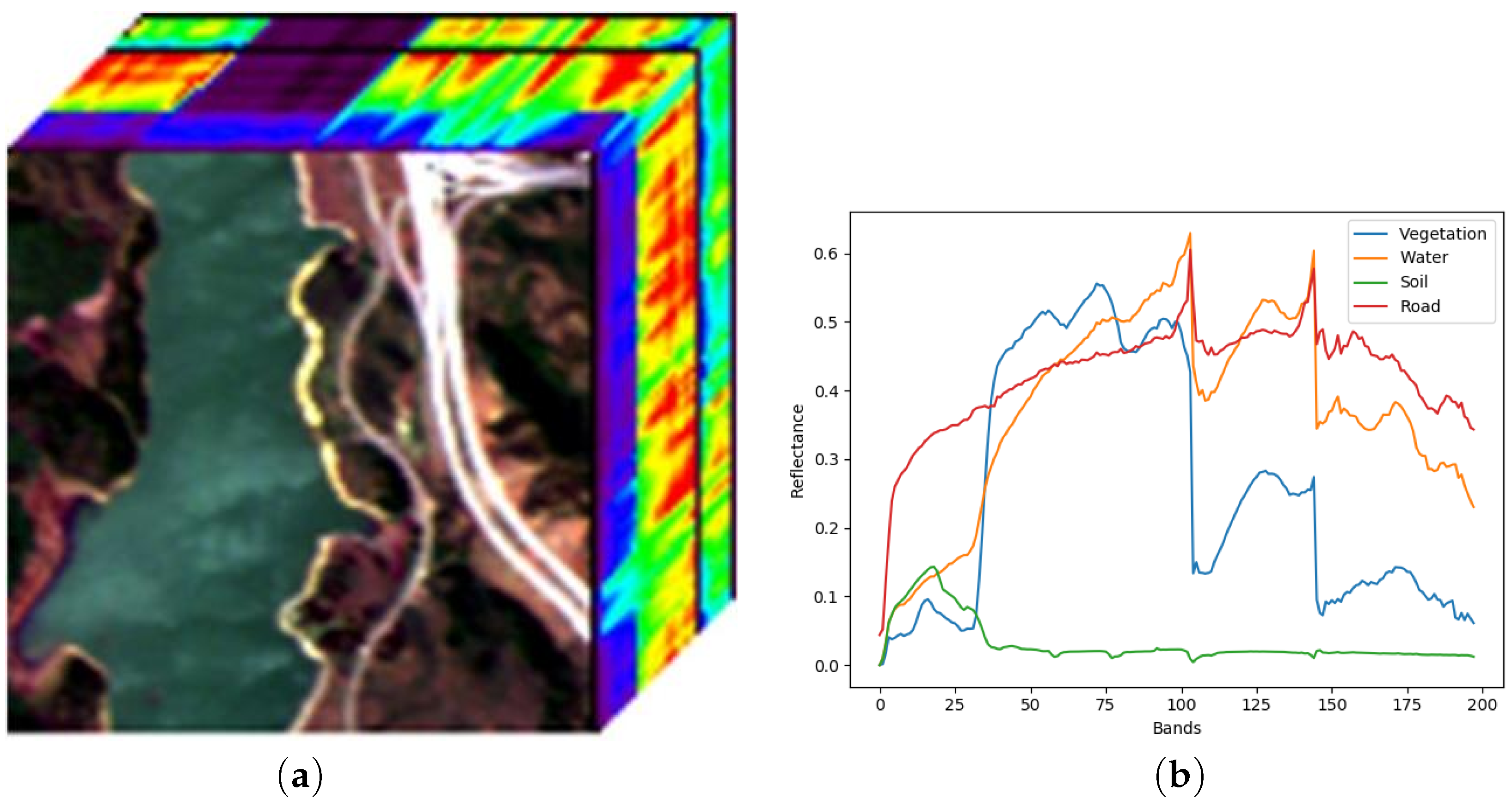
Hyperspectral imaging allows the acquisition of multivariate images containing information in hundreds of narrow and contiguous spectral bands [1], where each image pixel is a full-spectrum measurement of an area of the surface. Since many surface materials have unique spectral features, the technique can detect and identify surface materials via a comparison of a spectrum sample with diagnostic spectra obtained from known materials. Hyperspectral imaging has been widely used in various fields, such as geological mapping, plant cover and soil studies, atmospheric research, environmental monitoring, and so on. However, due to the limitation of the spatial resolution of remote sensing devices and the complexity and diversity of surface objects, the spectrum of pixels, i.e., the data from imaging a portion of the surface under study will often contain spectral contributions from more than a single material. Such mixed pixels commonly exist in remote sensing images and significantly degrade the classification accuracy of hyperspectral images and the detection of specific target materials [2]. In order to improve the accuracy of remote sensing applications, spectral unmixing (SU) is necessary; the spectrum of a mixed pixel must be decomposed and represented as a mix of spectra, called endmembers, generated by component materials, and the respective proportions, called abundances, of their contributions to the spectrum of the mixed pixel.

Any SU technique depends on understanding (or assuming) the mechanism of spectral mixing. There are two common types of spectral mixing models: linear mixing models and nonlinear mixing models. Because of the simple principle and clear physical meaning of the linear spectral mixing model, most of the early spectral unmixing methods were proposed based on the linear mixing model. Spectral unmixing using linear mixing models is accomplished in two steps. The first step is to extract endmembers; typical endmember-extraction methods include the N-FINDR algorithm [3], the simplex growing algorithm (SGA) [4], and vertex component analysis (VCA) [5]. The second step is to perform abundance inversion based on endmember and spectral data, and the common method is the fully constrained least squares method (FCLS) [6]. The linear mixing model is suitable for ground objects that are essentially linear mixtures and ground objects that can be considered linear mixtures on a large scale.

For the fine spectral analysis of some micro-scale ground objects or the identification of some low-probability targets, a nonlinear mixing model is required. Several typical nonlinear mixing models have been proposed, for example, the Fan model [7], the Nascimento model [8], the Hapke model [9], the generalized bilinear model (GBM) [10], and the post-nonlinear mixed model [11]. These better explain the multiple scattering and mixing of photons from ground objects in complex scenes.

The endmember is susceptible to variation due to the influence of atmosphere, illumination, terrain, and the intrinsic variability in the endmember [12]. The variations affect the accuracy of unmixing and the robustness of unmixing algorithms. Therefore, large efforts have recently been dedicated to mitigating the effects of spectral variability in SU.

Spectral unmixing methods based on the nonlinear mixing model perform well for some scenes because the nonlinear mixing model can explain non-negligible spectral variabilities. However for various reasons, unmixing methods based on nonlinear models are not favored; such models have a large capacity that can lead to overfitting and poor controllability [13], and deep learning-based methods that account for endmember variability using nonlinear mixing models often lack interpretability, so the estimation of endmembers present at different locations in the scene is difficult [14]. Spectral variable unmixing studies typically use analysis methods that are based on linear mixing models. Studies have included the extended linear mixing model (ELMM) [15], the generalized linear mixing model (GLMM) [16], the perturbed linear mixing model (PLMM) [17], and the augmented linear mixing model (ALMM) [18]. The ELMM is provably obtainable from the Hapke model by continually simplifying physical assumptions [19]. By only taking scaling factors into account, the ELMM is incomplete because certain consequential spectral variabilities are not representable using only scaling factors. The ELMM can be extended for the GLMM by defining three-dimensional tensors. The GLMM allows for the consideration of band-dependent scaling factors for the endmember signatures and can represent a larger variety of realistic spectral variations of the endmembers [16]. The PLMM considers that, in the absence of any prior knowledge about variability [20], the variability is modeled using an additive perturbation term for each endmember [21]. The PLMM lacks a physical meaning because the spectral variability cannot be adequately represented by only an additional term. The ALMM addresses the limitations of the ELMM and PLMM models by considering the scaling factors and other spectral variability simultaneously, according to their distinctive properties; the alternating direction method of the multiplier is used to solve the mixing model.

Besides the spectral mixing model, the algorithm used to solve the model is also important. Compared with the traditional convex optimization algorithm, the method based on neural networks is more convenient and efficient to implement, and its convergence is also better. The autoencoder (AE) is a typical unsupervised deep learning network, which generally consists of an encoder and a decoder. The encoder can map the input into a hidden layer containing low-dimensional embedding (i.e., abundances), and the decoder can reconstruct the original input from low-dimensional embedding [22]. The AE method has the advantages of good convergence and easy solutions and is suitable for resolving the issues listed above. In recent years, the extensive in-depth study of AEs and their application has led to the proposal of a series of spectral unmixing algorithms based on AEs, such as non-negative sparse autoencoders (NNSAEs) [23], stacked non-negative sparse autoencoders (SNSAs) [24], deep learning autoencoder unmixing (DAEU) [25], and convolutional neural network autoencoder unmixing (CNNAEU) [26]. The output of the encoder of an ordinary AE is only a value that represents the attributes of the latent variable; the research on applications in hyperspectral unmixing has developed the variational autoencoder (VAE) [27], whose encoder outputs the probability distribution of each latent variable to make its results more representative.

1.1. Motivation

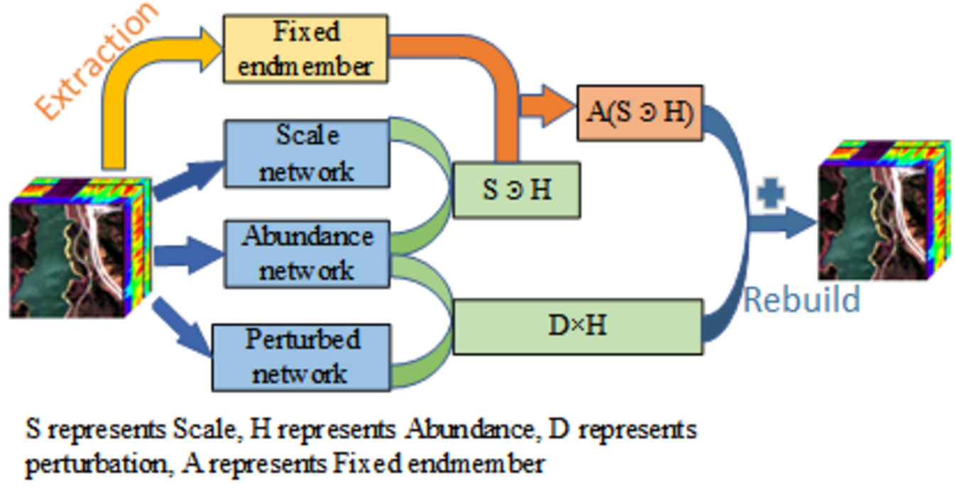
Although the ALMM effectively overcomes the deficiencies, the model is difficult to implement with deep learning networks because there are more unknown terms to be solved than with other models. The scale factor and additive perturbation complement each other to better fit the target spectrum [28]. This paper comprehensively considers the factors of spectral variability and combines the common ELMM and PLMM into a new scaled and perturbed linear mixing model (SPLMM), which, unlike the ALMM, can be efficiently solved using end-to-end neural networks.

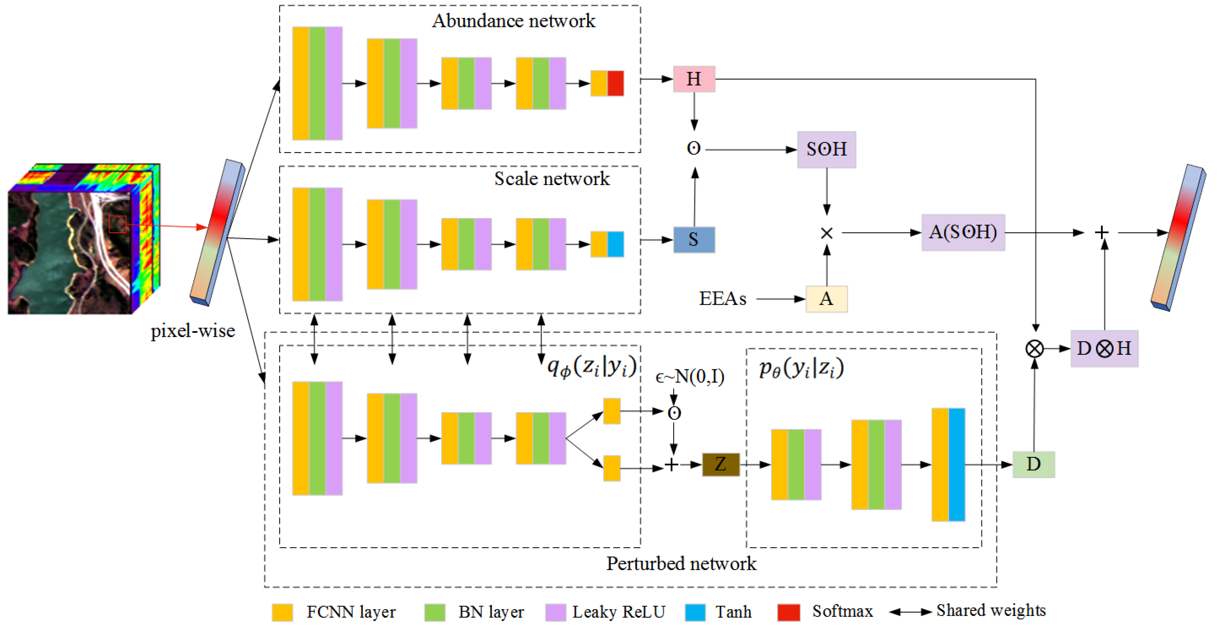
PLMM assumes that spectral variability follows a Gaussian distribution [18], which is not strictly true in real scenarios. The Probabilistic Generative Model for Hyperspectral Unmixing (PGMSU) [14] can approximate arbitrary endmember distributions and so address endmember variability, allowing the fitting of arbitrary endmember distributions through the nonlinear modeling capability of VAEs [29]. Drawing on the ideas behind the PGMSU, a network for the proposed SPLMM is constructed, which simultaneously solves the abundances, scales, and approximate arbitrary perturbation distributions. Suitable constraints on scale and perturbations are added to enhance the robustness of the model, and the sparse constraint of abundance is added to prevent overfitting.

1.2. Contributions

The specific contributions of this paper are summarized as follows:

• We propose a new spectral mixing model, SPLMM, and a corresponding solving network. SPLMM comprehensively considers the influence of scale and perturbation factors and better explains the variability of endmembers. Using the neural network to solve the model not only reduces the use of parameters but also makes the model more convenient and efficient to implement, and the convergence to the solution is improved.
• We propose a new network modeling method to enhance the estimation of endmembers. Determining the initial fixed endmembers by extracting endmembers, using the fully connected neural network to construct the scale, and using the nonlinear modeling ability of the VAE to fit any perturbation distribution, which not only limits the range of endmembers but also better fits various situations of variable endmembers.
• We propose adding various regularization constraints. The spatial smoothness constraint is added to the scale, and the regularization constraint is added to the perturbation, which improves the robustness of the model. For abundance, adding sparse constraints helps prevent overfitting.

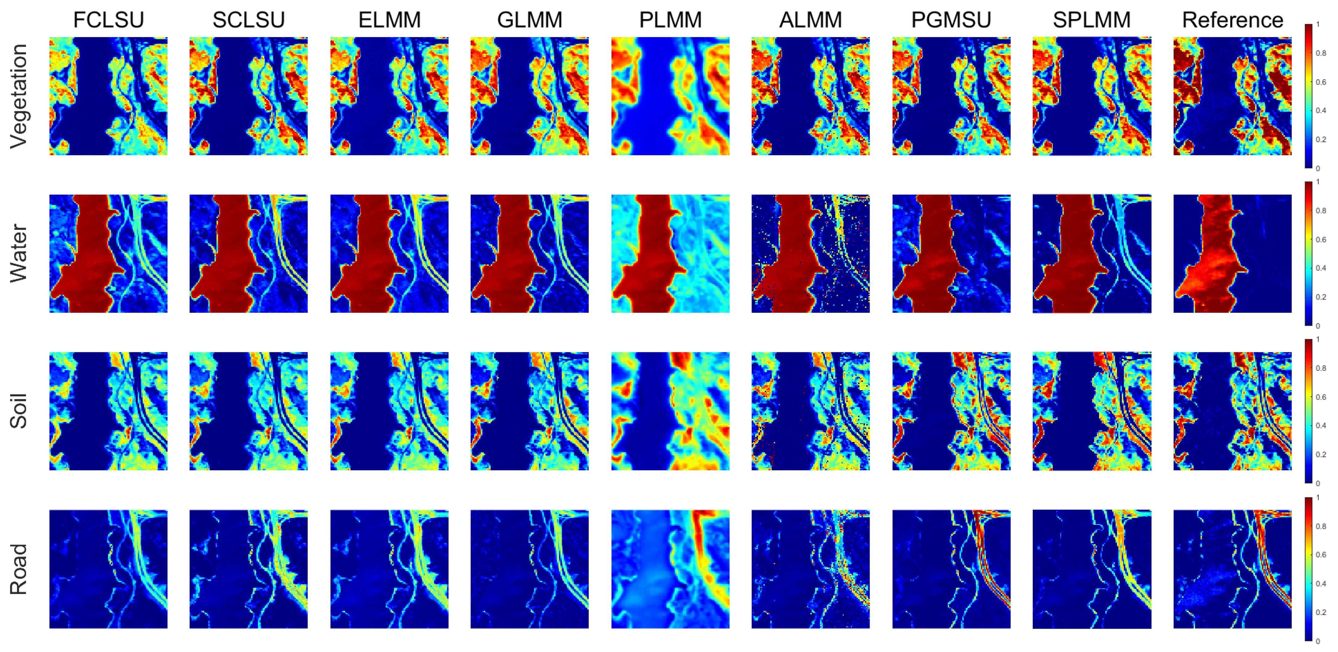
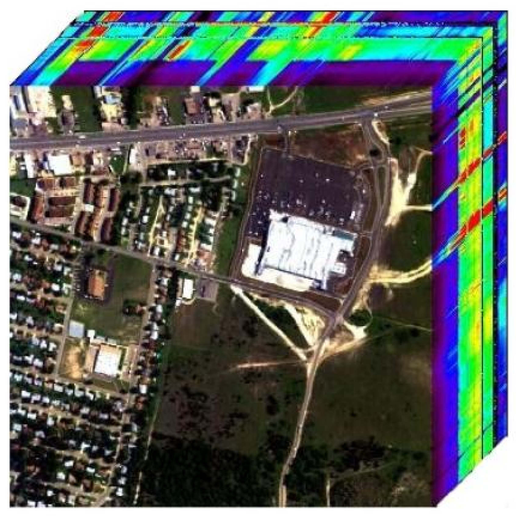
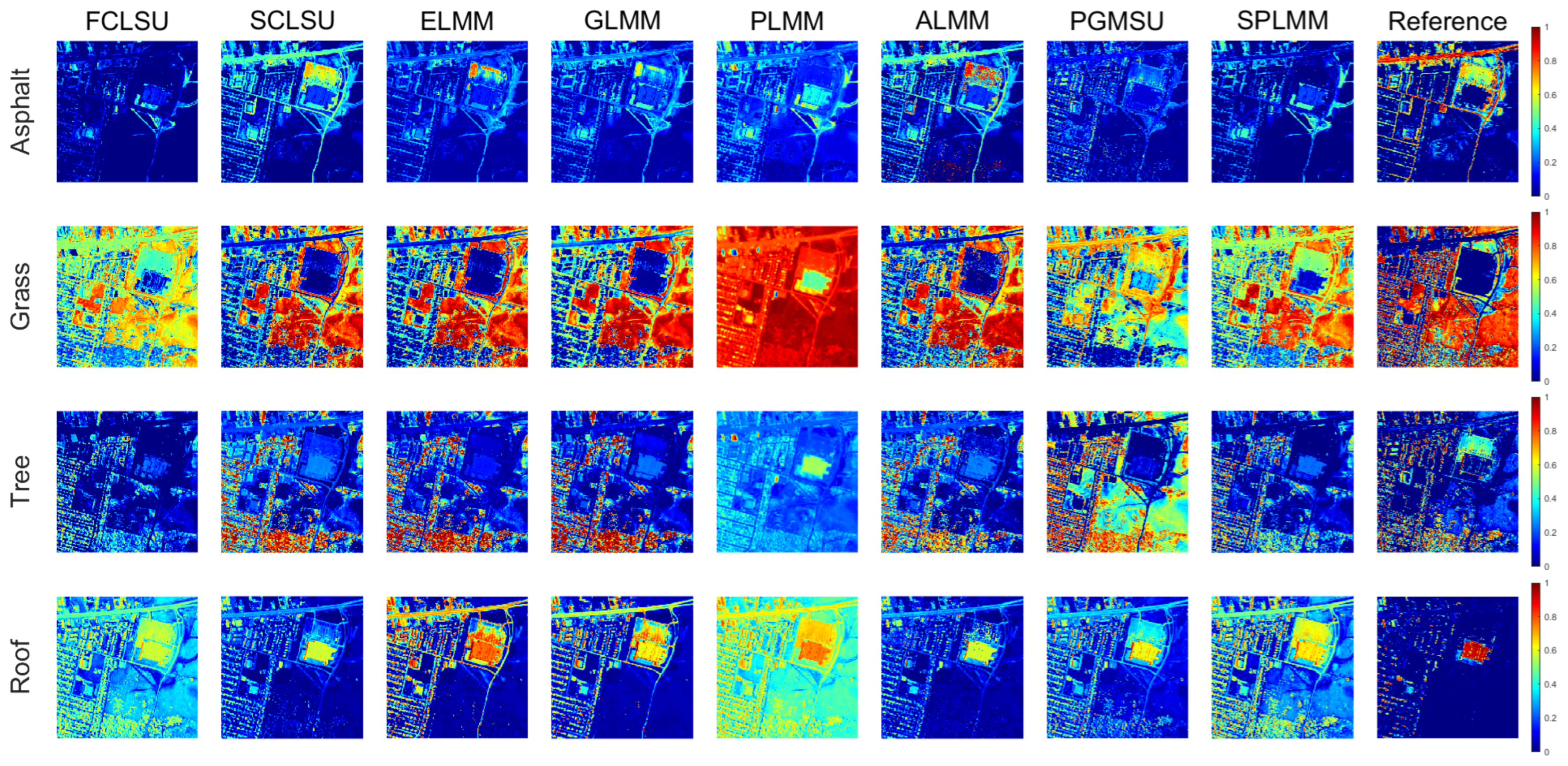
The organization of this article is as follows. Section 2 describes works related to the theoretical analysis of the proposed SPLMM. Section 3 presents the proposed model and its implementation details. Section 4 introduces experimental results and comparisons. Finally, Section 5 presents conclusions.

2. Related Work

In this section, we introduce the linear mixing model, the ELMM and the PLMM, and then briefly introduce the VAE.

2.1. Linear Mixing Model

The linear mixing model (LMM) assumes that each pixel spectrum is a linear combination of the several contributing endmembers, each weighted by its corresponding fractional abundance and summed into the image pixel [30]. Considering the influence of the abundance sum-to-one constraint (ASC) and the abundance non-negativity constraint (ANC), the LMM is described for the observed pixel as follows:

$$y_i=A{h}_i+r_i,1^T{h}_i=1,h_i\ge 0,{\forall }_i$$

(1)

where $y_i\in {\mathbb{R}}^L$ denotes the observed mixed pixel spectrum, L is the number of spectral bands, $A\in {\mathbb{R}}^{L\times P}$ represents the endmember matrix, P is the number of endmembers, $h_i\in {\mathbb{R}}^P$ represents the abundance vector corresponding to the ith pixel spectrum, and $r_i\in {\mathbb{R}}^L$ represents model error or the Gaussian noise.

2.2. Extended Linear Mixing Model

In the ELMM, the contributing endmembers are allowed to vary in each pixel spectrum, and the mixing process remains linear. The variability of the endmembers can be modeled by using scaling factors; the mechanism is expressed as follows:

$$y_i={\sum }_{p=1}^P{a}_p{s}_{p,i}{h}_{p,i}+r_i$$

(2)

where $s_{p,i}$ is a positive scaling factor whose effect is to locally rescale each endmember, $h_{p,i}$ is the abundance coefficient for material p at pixel i, $a_p$ is a reference endmember spectrum for material p, and $r_i$ is additive noise. The overall expression is as follows:

$$Y=A(S\odot H)+R$$

(3)

where $Y\in {\mathbb{R}}^{L\times N}$ represents the pixel matrix, $S\in {\mathbb{R}}^{P\times N}$ represents the scale matrix, $H\in {\mathbb{R}}^{P\times N}$ represents the abundance matrix, and $R\in {\mathbb{R}}^{L\times N}$ is additive noise. The operator ⊙ denotes the Hadamard product.

2.3. Perturbed Linear Mixing Model

In the PLMM, the variability in the endmembers is modeled by applying additive perturbation to the spectra of endmembers contributing to each pixel spectrum, which is expressed as follows:

$$y_i={\sum }_{p=1}^P\left(a_p+d_{p,i}\right)h_{p,i}+r_i$$

(4)

where $d_{p,i}\in {\mathbb{R}}^L$ is a perturbation vector, which represents the additive spectral perturbation of the pth endmember of the ith pixel spectrum. The set of variability terms $d_{p,i}(p=1,\dots ,P,i=1,\dots ,N)$ are gathered in the 3-D array $D\in {\mathbb{R}}^{L\times P\times N}$. The overall expression is as follows:

$$Y=\mathcal{M}\otimes H+R$$

(5)

where $\mathcal{M}\in {\mathbb{R}}^{L\times P\times N}$ is a 3-D array of the pixelwise perturbed endmember spectrum, $\mathcal{M}\otimes H=[M_1{h}_1,\dots M_i{h}_i,\dots M_N{h}_N]$, $M_i\in {\mathbb{R}}^{L\times N}$ represents the perturbed endmember spectrum, and $M_i=A+D_{:,:,i}$. The operator ⊗ represents the tensor product of matrixes and vectors.

2.4. Variational Autoencoders

A Variational Autoencoder (VAE) is a generative model using variational inference, and it was first proposed by Kingma et al. [31]. Its basic principles are briefly described as follows. The VAE is divided into two parts: encoder and decoder. The encoder encodes the input data y into hidden layer data $z=encoder\left(y\right)\sim q\left(z\right|y)$, through training; the VAE calculates the mean value $\mu$ and standard deviation $\sigma$, making it follow the Gaussian distribution. Then, through the decoder, the hidden layer data z are reconstructed into the input data $\widehat{y}=decoder\left(z\right)\sim p\left(y\right|z)$. The loss function of the VAE is composed of two parts [32]: reconstruction loss ${\mathcal{L}}_{rec}$ and Kullback–Leibler (KL) divergence ${\mathcal{L}}_{kl}$.

$${\mathcal{L}}_{vae}={\mathcal{L}}_{rec}+{\mathcal{L}}_{kl}$$

(6)

$${\mathcal{L}}_{\mathrm{rec}}=E_{q(z\mid y)}[logp(y\mid z)]=\frac{1}{N}{\sum }_{i=1}^N{\left(y_i-{\widehat{y}}_i\right)}^2$$

(7)

$${\mathcal{L}}_{kl}=-KL(q(z\mid y)\parallel p\left(z\right))$$

(8)

where the mean square error is used to measure the reconstruction loss of VAE, and $p\left(z\right)$ is the prior distribution of the latent space, set to be a standard normal distribution.

3. Proposed Model

3.1. Scaled and Perturbed Linear Mixing Model

In combining scale factors and additive perturbations, the SPLMM model is proposed, and the ith pixel spectrum $y_i\in {\mathbb{R}}^L$ is reconstructed as follows:

$$y_i=(A{s}_i+d_i)h_i$$

(9)

where $s_i\in {\mathbb{R}}^P$, $d_i=D_{:,:,i}\in {\mathbb{R}}^{L\times P}$ and $h_i\in {\mathbb{R}}^P$ denote the scale vector, perturbation matrix, and abundance vector for the ith pixel, respectively. The overall expression is as follows:

$$Y=A(S\odot H)+D\otimes H, 0\le H\le 1, A\ge 0$$

(10)

where $Y\in {\mathbb{R}}^{L\times N}$ represents the pixel matrix, $A\in {\mathbb{R}}^{L\times P}$ represents the fixed endmember matrix obtained by endmember extraction algorithms (EEAs), $H\in {\mathbb{R}}^{P\times N}$ represents the abundance matrix, $S\in {\mathbb{R}}^{P\times N}$ represents the scale matrix, and $D\in {\mathbb{R}}^{L\times P\times N}$ represents the perturbation. $D\otimes H=[d_1{h}_1,\dots d_i{h}_i,\dots d_N{h}_N]$.

3.2. Spectral Unmixing Based on SPLMM

The network structure of the SPLMM unmixing algorithm is shown in Figure 1, where a multi-stream deep learning architecture [33] is used to build abundances, scales, and perturbations. The network configuration is shown in

Table 1. Network configuration table of SPLMM.

Abundance Network		Scale Network		Perturbed Network
Layers	neurons	Layers	neurons	Layers	neurons
FC1–BN1–LReLU	32P	FC1–BN1–LReLU	32P	FC1–BN1–LReLU	32P
FC2–BN2–LReLU	16P	FC2–BN2–LReLU	16P	FC2–BN2–LReLU	16P
FC3–BN3–LReLU	4P	FC3–BN3–LReLU	4P	FC3–BN3–LReLU	4P
FC4–BN4–LReLU	4P	FC4–BN4–LReLU	4P	FC4–BN4–LReLU	4P
FC5–softmax	P	FC5–tanh	P	FC5	P
–	–	–	–	FC6	P
–	–	–	–	FC7–BN7–LReLU	16P
–	–	–	–	FC8–BN8–LReLU	64P
–	–	–	–	FC9–tanh	LP

, where, in the layer names, $F{C}_i$ represents the fully connected layer of the ith layer, $B{N}_i$ represents the batch normalization layer of the ith layer, LReLU represents the Leaky ReLU activation function, tanh represents the tanh function, and softmax represents the softmax function.

3.3. Design of the Abundance Network, Scale Network, Perturbed Network, and Loss Function

3.3.1. The Abundance Network

The abundance network is used to estimate the abundance term, and using a nonlinear function to directly map pixels to abundance for each pixel, the process can be expressed as

$$h_i=f_{\phi }\left(y_i\right)$$

(11)

where $f_{\phi }(·)$ is a nonlinear function parameterized by $\phi$. The abundance network is mainly modeled using fully connected networks (FCNNs). The data are input into an FCNN with the number of input nodes set to the number of bands, and the number of output nodes is gradually reduced to ensure that the number of output nodes in the last layer is equal to the dimension of abundance. Except for the last layer, the output layer of each FCNN tracks a batch-normalization layer (BN) [34] to speed parameter learning. The activation functions used in this experiment are the Leaky ReLU functions [35]. Compared with the ReLU function, the Leaky ReLU function has better fitting ability and is more suitable for processing high-dimensional data. In order to ensure the abundance of the output satisfying the ANC and ASC constraints, the last layer of FCNN uses the softmax function as the final output layer.

3.3.2. The Scale Network

The scale network is used to estimate the scale factors using a nonlinear function to directly map pixels to scale. The process can be expressed as:

$$s_i=f_{\varphi }\left(y_i\right)$$

(12)

where $f_{\varphi }(·)$ is a nonlinear function parameterized by $\varphi$. The scale network is also realized by FCNNs. Like the abundance network, the first few FCNNs track a BN layer to speed up the learning speed and a Leaky ReLU function as the activation function layer. The tanh function is used for the scale to control the range of the output scale item and effectively prevent overfitting; the function is expressed as

$$tanh\left(x\right)=\frac{e^x-e^{-x}}{e^x+e^{-x}}$$

(13)

3.3.3. The Perturbed Network

The perturbed network is realized by VAEs. First, we introduce a vector for each pixel, which is the latent representation of the perturbation of endmembers, encoding their variability. For each pixel, this is expressed as

$$d_i=f_{\theta }\left(z_i\right)$$

(14)

where $f_{\theta }(·)$ is a nonlinear function parameterized by $\theta$. In brief, the generative process of the perturbations can be formulated as Equation (14). The perturbed network can be realized by using FCNNs tracked with the BN layer and the Leaky ReLU activation. The last layer of the FCNN uses the tanh function as the final output layer, which limits the produced perturbations to a certain range by multiplying by a threshold value.

Second, we use a neural network $q_{\varphi }$ parameterized by $\varphi$ as an approximation of the true posterior distribution of the latent vector $z_i$ conditioned on the pixel $y_i$. The posterior distribution is approximated using a Gaussian as follows:

$$q_{\varphi }\left(z_i\right|y_i)=\mathcal{N}({\mu }_z,{\Sigma }_z)$$

(15)

where ${\Sigma }_z=diag\left({\sigma }_z^2\right)$ is a diagonal covariance matrix, and ${\mu }_z$ and ${\sigma }_z^2$ are the mean and variance of the latent variable $z_i$, respectively. The FCNN with the pixel as input is also used to model the mean and covariance diagonal matrices of the Gaussian distribution in Equation (15). Considering that both the scale and the perturbation are part of the variable endmembers, the weights of these two parts are shared, so they use the same parameter $\varphi$. This design not only reduces the number of parameters, but also reduces the complexity of the model and improves the efficiency of the model. The encoder network structure is the same as the scale network structure.

Finally, after optimizing the parameters and inferring the latent variables, the scales and abundances according to Equation (10) are reconstructed for the observed pixels.

3.3.4. Loss Function

In order to ensure the consistency between the input pixel and its corresponding reconstructed pixel, according to Equation (9), the reconstruction error can be expressed as

$${\mathcal{L}}_{rec}=\left|\right|y_i-\widehat{y_i}{\left|\right|}^2=\left|\right|y_i-(A{s}_i+d_i)h_i{\left|\right|}^2$$

(16)

According to Equation (8), the KL divergence of the posterior distribution and the prior distribution can be expressed as

$${\mathcal{L}}_{kl}={\sum }_{i=1}^P-\frac{1}{2}[log{\Sigma }_z-{\mu }_z^2-{\Sigma }_z^2+1]$$

(17)

In actual remote sensing images, the selection of scale factors may need to consider various factors, such as the influence of terrain and atmosphere. In this paper, the spatial smoothing item is selected to constrain the scale, which can effectively reduce the outliers of the data and maintain the spatial consistency; the regular term is expressed as follows:

$${\mathcal{L}}_s=\frac{1}{2}\left(\right||{\mathcal{H}}_h{\left(S\right)\left|\right|}_F^2+\left|\right|{\mathcal{H}}_v{\left(S\right)\left|\right|}_F^2)$$

(18)

where ${\mathcal{H}}_h$, ${\mathcal{H}}_v$: ${\mathbb{R}}^{P\times N}$→${\mathbb{R}}^{P\times N}$ are linear operators of horizontal and vertical gradients between adjacent pixels (acting separately on each endmember).

In actual remote sensing images, the perturbations are usually similar in space. If the perturbations are simply added, the model may be affected by the perturbations, thereby reducing the accuracy. Here, it is prudent to consider adding the following regular items to the perturbations to improve the robustness of the model:

$${\mathcal{L}}_d=\frac{1}{2}{\left|\right|D\left|\right|}_F^2$$

(19)

In hyperspectral images, sparsity is an important property. This means that most of the pixels exist as pure pixels, and only a few pixels contain multiple ground features [30]. In these sparse images, each abundance of each endmember is locally distributed, and the abundance has a certain sparsity, so it is necessary to introduce regularization sparsity constraints. The regular term chosen in this article is $L_{1/2}$, which is more easily generalized than $L_1$ and helps prevent overfitting.

$${\mathcal{L}}_h={\sum }_{i=1}^P\left|\right|H_{i,:}{\left|\right|}_{1/2}$$

(20)

At present, considering the constraints of Equations (16)–(18) and (20), the obtained objective function can be expressed as

$$\mathcal{L}={\mathcal{L}}_{rec}+{\lambda }_{kl}{\mathcal{L}}_{kl}+{\lambda }_s{\mathcal{L}}_s+{\lambda }_h{\mathcal{L}}_h$$

(21)

To sum up, the SPLMM procedure [36] is shown in Algorithm 1.

Algorithm 1. SPLMM: Global Algorithm

Input: observed pixels: Y, fixed endmembers: A;

hyperparameters: ${\lambda }_{kl}$, ${\lambda }_s$, ${\lambda }_h$;

mini-batch size: m, numbers of batches $N/m$;

epochs: maxIter = 1000;

learning rate: $\eta$ = 0.001;

Output: abundances H, scales S, perturbations D;

Initialization: $\Theta =\left\{\phi ,\varphi ,\theta \right\}$, $k=0$, $i=$0;

Training stage:

1: While $k<maxIter$ do

2:       For $i<N/m$ do

3:             Sample from Y

4:             Update H using Equation (11)

5:             Update S using Equation (12)

6:             Update D using Equations (14) and (15)

7:             Compute $\widehat{Y}$ using Equation (10)

8:             Compute Loss $\mathcal{L}(\Theta )$ using Equation (21)

9:             Back propagation

10:            $i=i+1$

11:       end

12:       $k=k+1$

13: end

Test stage:

14: Forward propagation: Feed the SPLMM Y;

15: Obtain H, S, and D

4. Experiments

The methods used in the comparative experiments include the proposed method, SPLMM, and these legacy methods: FCLSU [6], scaled constrained least-squares unmixing (SCLSU) [37], ELMM [15], GLMM [16], PLMM [17], ALMM [18], and PGMSU [14]. The number of endmembers is assumed to be a priori knowledge. The proposed algorithm is implemented on the Pytorch framework and uses small-batch stochastic gradient descent to learn model parameters. Following Equations (11)–(15), the parameters set in the model are $\Theta =\left\{\phi ,\varphi ,\theta \right\}$, which are initialized using random sampling from the Xavier uniform distribution [38]. We adopt the Adam optimizer, and the learning rate is set to 0.001. We set the maximum number of iterations to 1000 with mini-batch size setting to m.

4.1. The Criteria of Algorithm Performance

For abundance, we consider the commonly used average root mean square error of abundance (aRMSE):

$$aRMSE=\frac{1}{N}{\sum }_{i=1}^N\sqrt{\frac{1}{P}\left|\right|h_i-\widehat{h_i}{\left|\right|}^2}$$

(22)

The estimation performance in terms of endmembers is evaluated by computing the endmember root mean square error (eRMSE) and the endmember spectral angular distance (eSAD):

$$eRMSE=\frac{1}{NP}{\sum }_{i=1}^N{\sum }_{j=1}^P\sqrt{\frac{1}{L}\left|\right|a_{ij}-\widehat{a_{ij}}{\left|\right|}^2}$$

(23)

$$eSAD=\frac{1}{NP}{\sum }_{i=1}^N{\sum }_{j=1}^{P}arccos\frac{a_{ij}^T\widehat{a_{ij}}}{\left|\right|a_{ij}\left|\right|\left|\right|\widehat{a_{ij}}\left|\right|}$$

(24)

If there is no ground-truth abundance and endmember, for most real data, we can consider the reconstruction’s overall root mean square error (rRMSE):

$$rRMSE=\frac{1}{N}{\sum }_{i=1}^N{\sum }_{j=1}^P\sqrt{\frac{1}{L}\left|\right|y_i-\widehat{y_i}{\left|\right|}^2}$$

(25)

4.2. Experiments on the Synthetic Data Set

4.2.1. Synthetic Data Set

A test image was generated to test the SPLMM method and compare the SPLMM method with other methods. The spectra used in this experiment were supplied by the DIRSIG spectral library. As is shown in Figure 2, muddy spectra, grass spectra, concrete spectra, and asphalt spectra were first sampled into 178 bands and then used to simulate an image with a size of 100 × 100 pixels. The abundance of each pixel was generated using the Hyperspectral Data Retrieval and Analysis tools, which were available at http://www.ehu.es/ccwintco (accessed on 3 March 2023). Finally, a signal-to-noise ratio of 30 dB Gaussian noise was added to the mixed pixels. The synthetic image is displayed in Figure 3.

4.2.2. Design of Model

A.

Parameter Analysis

As the performance of the proposed method is sensitive to the hyperparameters, it is indispensable to conduct further parameter analysis for the selection of hyperparameters ${\lambda }_{kl}$, ${\lambda }_s$, and ${\lambda }_h$. According to the initial loss values $L_{rec}=2.86$, $L_{kl}=1.82$, $L_s=0.04$, and $L_h=1.91$, ${\lambda }_{kl}$ and ${\lambda }_s$ are fixed as $0.1$ and 5, respectively, and ${\lambda }_h$ is set as $[0:0.1:1]$. As is shown in Figure 4a, the best case can be obtained when ${\lambda }_h=0.2$. Then, ${\lambda }_h$ is fixed as $0.2$, and ${\lambda }_{kl}$ is set as $[0:0.1:1]$. Figure 4b shows that each result reached the most optimal value when ${\lambda }_{kl}=0.4$. Subsequently, ${\lambda }_{kl}$ and ${\lambda }_h$ are fixed as $0.4$ and $0.2$, respectively, and ${\lambda }_s$ is set as $[1:1:10]$. By inspecting Figure 4c, the best performance can be achieved by setting ${\lambda }_s$ as 5. Finally, the hyperparameters were set to ${\lambda }_{kl}=0.4$, ${\lambda }_h=0.2$, and ${\lambda }_s=5$.

Following Equation (21) and in accordance with Algorithm 1, the hyperparameters were set to ${\lambda }_{kl}=0.4$, ${\lambda }_s=5$, and ${\lambda }_h=0.2$. Keeping all the conditions of the run constant and changing only the number of iterations, the unmixing results under different numbers of iterations are shown in Figure 5. By inspecting Figure 5a, a relatively stable and better result is obtained after 300 iterations rather than 1000 iterations. As Figure 5b shows, the loss gradually converges when the iteration number is less than 100. The iteration is stopped when the loss changes for 20 consecutive iterations are within the specified interval of $[-0.004,0.004]$. According to the stopping condition for iteration, the final iteration number is less than 400.

B.

Neural Network Configuration

Following Equation (21) and in accordance with Algorithm 1, the hyperparameters were set to ${\lambda }_{kl}=0.4$, ${\lambda }_s=5$, and ${\lambda }_h=0.2$. Keeping the used data and fixed endmember unchanged, we set the number of runs to 1000 epochs. The evaluation index uses the aRMSE and the rRMSE. The results obtained under different network configurations are shown in

Table 2. Results under different network configurations.

Abundance Network	Scale Perturbation Network	aRMSE (${10}^{-2}$)	rRMSE (${10}^{-2}$)
32P–16P–P	32P–16P–P	10.63	1.09
32P–16P–4P–P	32P–16P–4P–P	8.88	1.07
32P–16P–4P–4P–P	32P–16P–4P–P	12.30	1.19
32P–16P–8P–4P–P	32P–16P–8P–4P–P	8.63	1.10
32P–16P–4P–4P–P	32P–16P–4P–4P–P	6.77	1.09
32P–16P–8P–4P–2P-P	32P–16P–8P–4P–2P-P	11.08	1.08

below.

According to the experimental results, the number of layers and the number of nodes in the abundance network and the scale-perturbation network have a certain influence on the values of aRMSE. When the number of network layers is the same, the values of rRMSE are similar. The network configuration given in the fifth scheme in the table has the smallest least-square error; the value is set in bold in the table.

C.

The Setting of the Loss Function

According to Equation (21), the loss function is composed of a reconstruction error, scale constraint, and abundance constraint. Comparing Equation (21) and the loss function with perturbation constraints added is instructive. The hyperparameters were set to ${\lambda }_{kl}=0.4$, ${\lambda }_s=5$, and ${\lambda }_h=0.2$. The results are shown in

Table 3. Results under Different Loss Functions.

Network Structure	Loss Function	aRMSE (${10}^{-2}$)	rRMSE (${10}^{-2}$)
AN + SN	$\mathcal{L}={\mathcal{L}}_{rec}+{\lambda }_s{\mathcal{L}}_s+{\lambda }_h{\mathcal{L}}_h$	8.18	1.07
AN + SN + PN	$\mathcal{L}={\mathcal{L}}_{rec}+{\lambda }_{kl}{\mathcal{L}}_{kl}+{\lambda }_s{\mathcal{L}}_s+{\lambda }_h{\mathcal{L}}_h$	6.77	1.09
	$\mathcal{L}={\mathcal{L}}_{rec}+{\lambda }_{kl}{\mathcal{L}}_{kl}+{\lambda }_s{\mathcal{L}}_s+{\lambda }_h{\mathcal{L}}_h+{\lambda }_d{\mathcal{L}}_d$	7.23	1.10

, where AN, SN, and PN represent the abundance network, the scale network, and the perturbation network, respectively. In these experimental results, the first line and the second line of the table, respectively, consider whether to add perturbation to the model, and the results show that the aRMSE of the added perturbation network is smaller, while rRMSE remains unchanged. The second and third lines consider whether to add perturbation constraints under the same mode, and the results show that the perturbation constraints do not work and that the result when not adding them is better; the reason may be that a threshold is added to the activation function of the perturbation, which limits the range of the perturbation, and adding constraints related to the disturbance value will not work. The loss function is designed as the second scheme in the table has the best performance (the smallest least-square error) and is set bold in the table.

4.2.3. Comparison Experiment Using the Synthetic Image

Table 4. Comparison of unmixing results of different methods on synthetic data.

Methods	aRMSE (${10}^{-2}$)	rRMSE (${10}^{-2}$)	eRMSE (${10}^{-2}$)	eSAD (${10}^{-2}$)	Tcpu (s)
VCA + FCLSU	7.38 ± 0.12	0.91 ± 0.02	1.43 ± 0.02	5.16 ± 0.14	1.31
SCLSU	9.78 ± 0.75	0.88 ± 0.02	1.87 ± 0.01	5.16 ± 0.14	1.30
ELMM	8.34 ± 0.23	0.82 ± 0.01	1.44 ± 0.02	5.14 ± 0.11	11.22
GLMM	8.11 ± 0.15	0.70 ± 0.01	1.44 ± 0.02	5.14 ± 0.11	25.61
PLMM	8.45 ± 0.45	0.17 ± 0.01	20.3 ± 0.06	34.1 ± 0.52	35.95
ALMM	9.07 ± 0.49	11.2 ± 0.06	–	–	36.52
PGMSU	6.05 ± 0.50	0.90 ± 0.02	1.49 ± 0.13	4.34 ± 0.31	92.53
SPLMM	6.02 ± 0.40	1.19 ± 0.04	1.51 ± 0.11	4.99 ± 0.15	69.25

lists the unmixing results of applying several methods to the synthetic image, and Figure 6 and Figure 7 show the abundance map and endmember bundle map of the unmixing results of the several methods as applied to the synthetic image. The results are analyzed in terms of several aspects below.

(1)

Analysis in Terms of Abundance

The comparison results of the quantitative performance of the several methods are presented in Table 4. Among them, SPLMM has the best estimation results for abundance. From the abundance estimation in Figure 6, the contrast between PGMSU and the proposed method is higher in terms of visual effects. The last two rows of the abundance map show that it is easy to confuse concrete and asphalt, and the reason may be that their features have some similarities. For these similar features, it may be difficult to distinguish one from the other, and it may be more effective to compare their probability distributions.

The visual comparison of the last column of the figure, the “true” image, with the SPLMM and PGMSU columns shows striking similarities, while the comparison of the true image with the second through fourth columns, all LMM methods, shows considerable visible error.

(2)

Analysis in Terms of Endmember

Considering the influence of the single endmember curve obtained using FCLSU and the spectral variation matrix in ALMM, the endmember diagrams of these two items are not drawn for comparison. The endmember bundle spectrum curves in Figure 7 show that the endmember spectra obtained using the proposed method are closest to the real endmember spectra. The endmember curves of PLMM are not smooth, and this implies that the perturbation obviously plays an important role. SPLMM results are compared to both PLMM and PGMSU, which succeed in flushing much of the “noise” introduced in the spectrum via the perturbation. The last two lines in Figure 7 show that the endmember curves are partially similar, which corresponds to the confusion of some substances in the abundance map in Figure 6. As shown in Table 4, it is worth noting that the numerical performance of SPLMM falls slightly short compared to PGMSU; this is mainly due to the fact that the errors of several spectral bands in the fourth endmember extracted using SPLMM are more significant compared with PGMSU. As a result, the eRMSE and eSAD of SPLMM slightly increase.

(3)

Analysis in Terms of Model Design

From the perspective of model design, the SPLMM achieves good unmixing results, benefiting from the following aspects: (1) Scale and perturbation factors are both considered to better explain the variability in endmembers. The weights share for the scale, and the perturbation not only reduces the number of parameters but also reduces the complexity of the model and improves the efficiency of the model. (2) The tanh function used in the scale network and the perturbations network can effectively prevent overfitting. (3) Using the nonlinear modeling ability of the VAE to fit any perturbation distribution can limit the range of endmembers and better fit various situations of variable endmembers. (4) For the loss function, the spatial smoothness constraint is added to the scale, and the regularization constraint is added to the perturbation, which improves the robustness of the model. For abundance, adding sparse constraints helps prevent overfitting.

4.3. Experiments on the Jasper Ridge Data Set

4.3.1. Jasper Ridge Data set

The JasperRidge data set collected from the AVIRIS sensor is 100 by 100 pixels, and each pixel contains 224 bands in the range of 0.38–2.5 µm. The obtained image of the data set is shown in Figure 8a. Due to the influence of water vapor and atmosphere, bands 1–3, 108–112, 154–166, and 220–224 were removed, and 198 bands were reserved for experiments. The data set mainly contains four kinds of endmembers, vegetation, water, soil, and road; their spectral curves are shown in Figure 8b.

4.3.2. Contrast experiment

Table 5. Comparison of unmixing results of different methods on the JasperRidge data set.

Methods	aRMSE (${10}^{-2}$)	rRMSE (${10}^{-2}$)	eRMSE (${10}^{-2}$)	eSAD (${10}^{-2}$)	Tcpu (s)
VCA + FCLSU	12.22 ± 0.43	1.32 ± 0.16	13.05 ± 0.59	15.63 ± 0.88	1.31
SCLSU	9.84 ± 1.18	1.15 ± 0.13	13.76 ± 0.26	15.63 ± 0.88	1.30
ELMM	9.86 ± 1.07	0.23 ± 0.01	12.87 ± 0.31	15.87 ± 0.86	10.81
GLMM	10.14 ± 0.84	0.11 ± 0.01	12.58 ± 0.33	13.38 ± 0.80	85.63
PLMM	11.09 ± 0.18	2.22 ± 0.01	3.34 ± 0.17	8.65 ± 0.24	42.95
ALMM	12.72 ± 3.91	21.9 ± 1.31	–	–	68.51
PGMSU	7.16 ± 0.19	1.66 ± 0.01	4.94 ± 0.06	6.14 ± 0.36	93.92
SPLMM	8.38 ± 0.35	1.62 ± 0.01	11.45 ± 0.40	14.96 ± 0.88	125.24

lists the unmixing results of different methods for the JasperRidge data set, and Figure 9 shows the abundance map of the JasperRidge data set’s unmixing results for different methods. The results are analyzed in several respects below.

(1)

Analysis in terms of abundance

Since the true abundance map of the JasperRidge data set is unknown, the obtained reference abundance map, which is available at http://rslab.ut.ac.ir/data (accessed on 23 March 2023), was used for algorithm evaluation, and the evaluation results of different methods are shown in Table 5. Like the synthetic data results, the abundance estimates of the proposed method are second only to the PGMSU. From the perspective of visualization, Figure 9 shows the abundance maps decomposed using different methods, which can be identified for the detection of vegetation and water, but when detecting water, except for PGMSU, the background purity of other methods is not high, showing the road. For soil detection, the results of the proposed method and PGMSU are more accurate, and our proposed method is closer to the reference abundance map. For road detection, only the contrast of PGMSU detection is more consistent.

(2)

Analysis in terms of pixels

Among the two methods with relatively good abundance estimation, the rRMSE obtained using our proposed method are better than the results of PGMSU. The results of PLMM and ALMM are relatively large, which may be due to the influence of the perturbation. The result of ELMM is smaller than the result of the proposed method, which is smaller than that of PLMM. The analysis shows that compared with ELMM, our proposed method adds perturbation, so the result is larger. Compared with PLMM, our proposed method adds scale, reducing the influence of the disturbance value, so the result is smaller.

4.4. Experiments on the Urban Data Set

4.4.1. Urban Data Set

The Urban Data set collected from the HYDICE sensor has 307 by 307 pixels, and each pixel contains 210 bands in the range of 0.4–2.5 µm. The image obtained from the data set is shown in Figure 10. Due to the influence of water vapor and atmosphere, bands 1–4, 76, 87, 101–111, 136–153, and 198–210 were removed, and 166 bands were reserved for experiments. The data set mainly contains four kinds of endmembers, asphalt, grass, tree, and roof.

4.4.2. Contrast Experiment

Table 6. Comparison of unmixing results of different methods on the urban data set.

Methods	aRMSE (${10}^{-2}$)	rRMSE (${10}^{-2}$)	Tcpu (s)
VCA + FCLSU	29.97 ± 3.14	6.78 ± 1.04	13.25
SCLSU	19.78 ± 1.01	1.47 ± 0.19	12.31
ELMM	23.19 ± 2.30	0.11 ± 0.03	601.10
GLMM	26.66 ± 7.37	0.06 ± 0.01	1624.33
PLMM	23.34 ± 0.51	0.78 ± 0.01	251.45
ALMM	37.09 ±1.76	18.69 ± 4.14	650.85
PGMSU	25.99 ± 1.95	1.48 ± 0.05	850.31
SPLMM	24.89 ± 2.22	5.15 ± 0.37	1022.45

lists the unmixing results of different methods for the urban data set, and Figure 11 shows the abundance maps of the urban data set’s unmixing results for different methods. The results are analyzed from several perspectives below.

(1)

Analysis in Terms of Abundance

Since the true abundance map of the urban data set is unknown, the obtained reference abundance map, which is available at http://rslab.ut.ac.ir/data (accessed on 23 March 2023), was used for algorithm evaluation, and the evaluation results of different methods are shown in Table 6. The aRMSE of the SCLSU is the smallest, and the results of ELMM and PLMM are similar to the proposed method. From the perspective of visualization, Figure 11 shows the abundance maps that were decomposed using different methods. For the detection of asphalt, the contrast of each method is not high, probably because the reflectivity of asphalt is low, and there are too many substances in the data set to accurately distinguish asphalt. Grass is the most distinguishable substance, and for the detection of trees, the contrast of the abundance map obtained with our proposed method is more consistent. For the detection of the roof, it may be because the endmember spectrum preprocessed using VCA did not accurately decompose the roof spectral curve, resulting in inaccurate detection of the roof with many methods.

(2)

Analysis in Terms of Pixel

According to Table 6, the results of ELMM and GLMM that only consider the scale are very great, while the results of PLMM that consider the perturbation are relatively poor. The reason may be that there are too many substances covered in the urban data set, and if perturbation is added, it is likely to confuse the substance and perturbation. The SPLMM adds scale and perturbation so that the spectral curve of each substance fits more possible spectral variations, the method is more likely in some scenarios to confuse substances, and the results obtained are worse.

5. Conclusions

In order to solve the spectral variable unmixing problem, a new linear mixing model named SPLMM is proposed, which explicitly accounts for the common factors of endmember variability. The unmixing algorithm for SPLMM is detailed and implemented in an unmixing network that introduces deep learning into the algorithm, connects the variational autoencoder, reduces the use of parameters, and can better converge the model. The spatial smoothness constraints of the scale and regularization constraints of the perturbation enhance the robustness of the model, and the sparse constraint of abundance is added to prevent overfitting. Experimental results using synthetic data and real data show that the algorithm we proposed can decompose the abundance map with higher contrast and more obvious discrimination, and the endmember bundle’s curve map is closer to the real situation, so the SPLMM method is comparable to, and can exceed, the performance of previous methods.

References

1. Borengasser, M.; Hungate, W.S.; Watkins, R. Hyperspectral Remote Sensing: Principles and Applications; CRC Press: Boca Raton, FL, USA, 2007. [Google Scholar]
2. Chengquan, C. Research on Hyperspectral Image Unmixing Technology; Higher Education Press: Beijing, China, 2019. [Google Scholar]
3. Winter, M.E. N-FINDR: An algorithm for fast autonomous spectral end-member determination in hyperspectral data. In Proceedings of the Spies International Symposium on Optical Science, Denver, CO, USA, 27 October 1999; Volume 3753, pp. 266–275. [Google Scholar]
4. Chang, C.I.; Wu, C.C.; Liu, W.; Ouyang, Y.C. A New Growing Method for Simplex-Based Endmember Extraction Algorithm. IEEE Trans. Geosci. Remote. Sens. 2006, 44, 2804–2819. [Google Scholar] [CrossRef]
5. Nascimento, J.M.; Dias, J.M. Vertex component analysis: A fast algorithm to unmix hyperspectral data. IEEE Trans. Geosci. Remote. Sens. 2005, 43, 898–910. [Google Scholar] [CrossRef] [Green Version]
6. Rhode, S.; Usevich, K.; Markovsky, I.; Gauterin, F. A recursive restricted total least-squares algorithm. IEEE Trans. Signal Process. 2014, 62, 5652–5662. [Google Scholar] [CrossRef] [Green Version]
7. Fan, W.; Hu, B.; Miller, J.; Li, M. Comparative study between a new nonlinear model and common linear model for analysing laboratory simulated-forest hyperspectral data. Int. J. Remote. Sens. 2009, 30, 2951–2962. [Google Scholar] [CrossRef]
8. Raksuntorn, N.; Du, Q. Nonlinear spectral mixture analysis for hyperspectral imagery in an unknown environment. IEEE Geosci. Remote. Sens. Lett. 2010, 7, 836–840. [Google Scholar] [CrossRef]
9. Hapke, B. Bidirectional reflectance spectroscopy: 1. Theory. J. Geophys. Res. Solid Earth 1981, 86, 3039–3054. [Google Scholar] [CrossRef] [Green Version]
10. Halimi, A.; Altmann, Y.; Dobigeon, N.; Tourneret, J.Y. Nonlinear unmixing of hyperspectral images using a generalized bilinear model. IEEE Trans. Geosci. Remote. Sens. 2011, 49, 4153–4162. [Google Scholar] [CrossRef] [Green Version]
11. Dobigeon, N.; Tourneret, J.Y.; Richard, C.; Bermudez, J.C.M.; McLaughlin, S.; Hero, A.O. Nonlinear unmixing of hyperspectral images: Models and algorithms. IEEE Signal Process. Mag. 2013, 31, 82–94. [Google Scholar] [CrossRef] [Green Version]
12. Chenghuan, Z. Research on Hyperspectral Image Unmixing Algorithm with Variable Endmembers; Hangzhou Dianzi University: Hangzhou, China, 2019. [Google Scholar]
13. Sen, F.; Wenjie, C.; Cheng, W. Multi-terminal hyperspectral image grouping optimal unmixing method based on extended linear model. Ship Electron. Countermeas. 2022, 45, 89–94. [Google Scholar]
14. Shi, S.; Zhao, M.; Zhang, L.; Altmann, Y.; Chen, J. Probabilistic generative model for hyperspectral unmixing accounting for endmember variability. IEEE Trans. Geosci. Remote. Sens. 2021, 60, 1–15. [Google Scholar] [CrossRef]
15. Drumetz, L.; Henrot, S.; Veganzones, M.A.; Chanussot, J.; Jutten, C. Blind hyperspectral unmixing using an extended linear mixing model to address spectral variability. In Proceedings of the 2015 7th Workshop on Hyperspectral Image and Signal Processing: Evolution in Remote Sensing (WHISPERS), Tokyo, Japan, 2–5 June 2015; pp. 1–4. [Google Scholar]
16. Imbiriba, T.; Borsoi, R.A.; Bermudez, J.C.M. Generalized linear mixing model accounting for endmember variability. In Proceedings of the 2018 IEEE International Conference on Acoustics, Speech and Signal Processing (ICASSP), Calgary, AB, Canada, 15–20 April 2018; pp. 1862–1866. [Google Scholar]
17. Thouvenin, P.A.; Dobigeon, N.; Tourneret, J.Y. Hyperspectral unmixing with spectral variability using a perturbed linear mixing model. IEEE Trans. Signal Process. 2015, 64, 525–538. [Google Scholar] [CrossRef] [Green Version]
18. Hong, D.; Yokoya, N.; Chanussot, J.; Zhu, X.X. An augmented linear mixing model to address spectral variability for hyperspectral unmixing. IEEE Trans. Image Process. 2018, 28, 1923–1938. [Google Scholar] [CrossRef] [PubMed] [Green Version]
19. Drumetz, L.; Chanussot, J.; Jutten, C. Spectral unmixing: A derivation of the extended linear mixing model from the Hapke model. IEEE Geosci. Remote. Sens. Lett. 2019, 17, 1866–1870. [Google Scholar] [CrossRef] [Green Version]
20. Jinliang, D. Inversion Model of Snow Coverage in Western Sichuan Plateau Based on Mixed Pixel Decomposition; Southwest Jiaotong University: Chengdu, China, 2021. [Google Scholar]
21. Johnson, E.C.; Jones, D.L. Joint recovery of sparse signals and parameter perturbations with parameterized measurement models. In Proceedings of the 2013 IEEE International Conference on Acoustics, Speech and Signal Processing, Vancouver, BC, Canada, 26–31 May 2013; pp. 5900–5904. [Google Scholar]
22. Su, L.; Liu, J.; Yuan, Y.; Chen, Q. A Multi-Attention Autoencoder for Hyperspectral Unmixing Based on the Extended Linear Mixing Model. Remote. Sens. 2023, 15, 2898. [Google Scholar] [CrossRef]
23. Lemme, A.; Reinhart, R.F.; Steil, J.J. Online learning and generalization of parts-based image representations by non-negative sparse autoencoders. Neural Netw. 2012, 33, 194–203. [Google Scholar] [CrossRef] [Green Version]
24. Su, Y.; Marinoni, A.; Li, J.; Plaza, J.; Gamba, P. Stacked nonnegative sparse autoencoders for robust hyperspectral unmixing. IEEE Geosci. Remote. Sens. Lett. 2018, 15, 1427–1431. [Google Scholar] [CrossRef]
25. Palsson, B.; Sigurdsson, J.; Sveinsson, J.R.; Ulfarsson, M.O. Hyperspectral unmixing using a neural network autoencoder. IEEE Access 2018, 6, 25646–25656. [Google Scholar] [CrossRef]
26. Palsson, B.; Ulfarsson, M.O.; Sveinsson, J.R. Convolutional autoencoder for spectral–spatial hyperspectral unmixing. IEEE Trans. Geosci. Remote. Sens. 2020, 59, 535–549. [Google Scholar] [CrossRef]
27. Ying, L. Research on Hyperspectral Image Fusion and Classification Based on Variational Probability Model; Xidian University: Xi’an, China, 2020. [Google Scholar]
28. Hua, Z.; Li, X.; Chen, S.; Zhao, L. Hyperspectral unmixing with scaled and perturbed linear mixing model to address spectral variability. J. Appl. Remote. Sens. 2020, 14, 026515. [Google Scholar] [CrossRef]
29. Zunxiong, L.; Yapeng, S.; Xiaoyu, P. Hyperspectral Image Classification Based on Two-Channel Variational Autoencoder. Comput. Eng. Appl. 2022, 58, 244–251. [Google Scholar]
30. Heinz, D.C. Fully constrained least squares linear spectral mixture analysis method for material quantification in hyperspectral imagery. IEEE Trans. Geosci. Remote. Sens. 2001, 39, 529–545. [Google Scholar] [CrossRef] [Green Version]
31. Kingma, D.P.; Welling, M. Auto-Encoding Variational Bayes. arXiv 2014, arXiv:1312.6114. [Google Scholar]
32. Ye, M.; Chen, J.; Xiong, F.; Qian, Y. Learning a deep structural subspace across hyperspectral scenes with cross-domain VAE. IEEE Trans. Geosci. Remote. Sens. 2022, 60, 1–13. [Google Scholar] [CrossRef]
33. Dian, R.; Shan, T.; He, W.; Liu, H. Spectral Super-Resolution via Model-Guided Cross-Fusion Network. IEEE Trans. Neural Netw. Learn. Syst. 2023, 1–12. [Google Scholar] [CrossRef]
34. Ioffe, S.; Szegedy, C. Batch normalization: Accelerating deep network training by reducing internal covariate shift. In Proceedings of the International Conference on Machine Learning, PMLR, Lille, France, 7–9 July 2015; pp. 448–456. [Google Scholar]
35. Xu, B.; Wang, N.; Chen, T.; Li, M. Empirical Evaluation of Rectified Activations in Convolutional Network. arXiv 2015, arXiv:1505.00853. [Google Scholar]
36. Dian, R.; Guo, A.; Li, S. Zero-Shot Hyperspectral Sharpening. IEEE Trans. Pattern Anal. Mach. Intell. 2023, 1–17. [Google Scholar] [CrossRef]
37. Veganzones, M.A.; Drumetz, L.; Tochon, G.; Dalla Mura, M.; Plaza, A.; Bioucas-Dias, J.; Chanussot, J. A new extended linear mixing model to address spectral variability. In Proceedings of the 2014 6th Workshop on Hyperspectral Image and Signal Processing: Evolution in Remote Sensing (WHISPERS), Lausanne, Switzerland, 24–27 June 2014; pp. 1–4. [Google Scholar]
38. Glorot, X.; Bengio, Y. Understanding the difficulty of training deep feedforward neural networks. In Proceedings of the Thirteenth International Conference on Artificial Intelligence and Statistics, Chia Laguna Resort, Sardinia, Italy, 13–15 May 2010; pp. 249–256. [Google Scholar]
Figure 1. Network structure diagram of the Scaled and Perturbed Linear Mixing Model (SPLMM).
Remotesensing 15 03890 g001
Figure 2. The four types of endmember spectra: (a) muddy, (b) grass, (c) concrete, (d) asphalt.
Remotesensing 15 03890 g002
Figure 3. Synthetic image.
Remotesensing 15 03890 g003
Figure 4. The result curves under different hyperparameters: (a) λ k l = 0.1 and λ s = 5 , (b) λ h = 0.2 and λ s = 5 , (c) λ k l = 0.4 , and λ h = 0.2 .
Remotesensing 15 03890 g004
Figure 5. The results under different iterations: (a) The performance, (b) The loss.
Remotesensing 15 03890 g005
Figure 6. Unmixed abundance maps of synthetic images using different methods.
Remotesensing 15 03890 g006
Figure 7. Endmember bundle diagrams of synthetic image unmixing using different methods.
Remotesensing 15 03890 g007
Figure 8. JasperRidge data set. (a) JasperRidge data set image, (b) Endmember spectral curves.
Remotesensing 15 03890 g008
Figure 9. Unmixed abundance maps of the JasperRidge data set obtained using different methods.
Remotesensing 15 03890 g009
Figure 10. Urban data set image.
Remotesensing 15 03890 g010
Figure 11. Unmixed abundance maps of the urban data set using different methods.
Remotesensing 15 03890 g011