Article

Spectral–Temporal Transformer for Hyperspectral Image Change Detection

Department of Electrical Engineering, Zhejiang University, Hangzhou 310027, China
*
Author to whom correspondence should be addressed.
Remote Sens. 2023, 15(14), 3561; https://doi.org/10.3390/rs15143561
Submission received: 19 May 2023 / Revised: 26 June 2023 / Accepted: 11 July 2023 / Published: 15 July 2023
(This article belongs to the Special Issue Advances in Hyperspectral Data Exploitation II)

Abstract

:
Deep-Learning-based (DL-based) approaches have achieved remarkable performance in hyperspectral image (HSI) change detection (CD). Convolutional Neural Networks (CNNs) are often employed to capture fine spatial features, but they do not effectively exploit the spectral sequence information. Furthermore, existing Siamese-based networks ignore the interaction of change information during feature extraction. To address this issue, we propose a novel architecture, the Spectral–Temporal Transformer (STT), which processes the HSI CD task from a completely sequential perspective. The STT concatenates feature embeddings in spectral order, establishing a global spectrum–time-receptive field that can learn different representative features between two bands regardless of spectral or temporal distance, thereby strengthening the learning of temporal change information. Via the multi-head self-attention mechanism, the STT is capable of capturing spectral–temporal features that are weighted and enriched with discriminative sequence information, such as inter-spectral correlations, variations, and time dependency. We conducted experiments on three HSI datasets, demonstrating the competitive performance of our proposed method. Specifically, the overall accuracy of the STT outperforms the second-best method by 0.08%, 0.68%, and 0.99% on the Farmland, Hermiston, and River datasets, respectively.

1. Introduction

Recently, hyperspectral images (HSIs) have received remarkable interest as a result of their numerous continuous spectral bands, large spectral range, and high spectral resolution. This prominent spectral resolution enables more precise observations of land cover, making HSIs invaluable resources for remote sensing change detection (CD). CD is the process used to identify and analyze differences between images of the same area taken at different times. This can be used for agricultural monitoring [1], resource exploration, land-change monitoring, potential anomaly identification [2,3,4], and various other applications. With the help of rich spectral information, HSI CD has the potential to identify finer changes.
Traditional CD methods for HSIs can be classified into three categories: (i) image algebra-based methods; (ii) image transformation; and (iii) classification-based methods. They obtain the similarities among HSI pixels by applying hand-crafted feature extraction techniques. Specifically, image algebra-based methods employ algebraic techniques, such as image difference [5] and image log ratio [6], to measure the difference in images and further generate a change detection map. Change Vector Analysis (CVA) [7] is a classical image algebra method that calculates the magnitude and direction between two pixels of bi-temporal images. Later, many variants of the CVA method were developed, such as Deep CVA (DCVA) [8] and Robust CVA (RCVA) [9], to improve detection performance. DCVA employs a pretrained Convolutional Neural Network (CNN) to extract deep features. To reduce spurious changes, RCVA accounts for pixel neighborhood effects. Image algebra methods are fast and easy to implement because they directly perform mathematical operations on the corresponding bands. Meanwhile, the simple operation makes them susceptible to imaging conditions and noise. Image-transformation-based methods transfer temporal variants into a specific feature space to identify the changes. Principal Component Analysis (PCA) [10] is utilized to reduce redundancy and noise within data while simultaneously extracting essential information and characteristics from HSIs. Multivariate Alteration Detection (MAD) utilizes canonical correlation analysis to transform the hyperspectral data into a new coordinate system to statistically detect changes [11]. Iterative Reweighted MAD (IR-MAD) [12] incorporates weights for each pixel based on the chi-squared distribution at every iteration to enhance change detection performance. By assigning appropriate weights, IR-MAD can effectively mitigate the influence of noisy or outlier pixels. Hou et al. [13] proposed a tensor-based framework, Tensor Decomposition and Reconstruction Detector (TDRD), which uses tensor representation and Tucker decomposition to extract high-level semantic information and remove the effects of irrelevant changes to improve accuracy. These image transformation methods are capable of enhancing the discrimination between changed and unchanged features by reducing dimension and noise. However, it is time-consuming to transform complicated images. Classification-based methods [14,15] compare the classification results of bi-temporal images to generate “from-to” change detection results. Therefore, the detection results are heavily dependent on the classification accuracy. In summary, these traditional methods exploit shallow features to generate change maps, resulting in a lack of robustness across different or complex scenes, and they do not easily select appropriate thresholds. In addition, these approaches do not consider the intrinsic connection between HSI bands and ignore the physical meaning of continuous spectral signatures.
To overcome the constraints of traditional methods, recent research has focused on integrating Deep Learning (DL) techniques with a particular emphasis on CNNs as powerful tools for HSI CD. Due to their ability to capture spatial semantic information effectively, CNNs have made remarkable progress in the domains of computer vision (CV) [16,17,18] and remote sensing [19,20,21]. Wang et al. [22] presented a two-dimensional (2D) CNN to integrate local information and learn meaningful features from a subpixel-represented, mixed-affinity matrix. With the help of CNN’s own structure, Saha et al. [23] extracted low-level semantic features from bi-temporal images without any training. In [24,25], both a one-dimensional (1D) CNN and a 2D CNN were used to explore spectral and spatial information, respectively. Zhan et al. [26] employed a three-dimensional (3D) CNN to extract tensor features and generate a change map with the similarity measurement of tensor pairs. Ou et al. [27] proposed a band selection strategy to alleviate band redundancy before feeding the difference image into a CNN-based framework. Wang et al. [28] designed self-calibrated convolution to make full use of inter-spatial and inter-spectral dependencies by heterogeneously exploiting convolutional filters. In [29], Zhao et al. extracted spatial–spectral features using a simplified autoencoder without requiring prior information. Seydi et al. [30] employed multi-dimensional convolution and depth-wise dilated convolution to extract different features. The above algorithms improved the accuracy of change detection by designing different network structures to effectively leverage spatial information. However, they compare the characteristics of bi-temporal images using difference [23,24,27] or concatenation [22,25,28,29,30] and are unable to learn temporal change information well. This becomes a key factor restricting further improvements in change detection accuracy.
Therefore, several researchers [31,32,33] introduced Recurrent Neural Networks (RNNs) to extract change information, and Long Short-Term Memory (LSTM) is most often used to overcome the problem of gradient vanishing. Lyu et al. [31] introduced RNNs to change detection to learn a change rule with good transferability for the first time. In [32], convolutional LSTM was employed to model temporal change information while maintaining the spatial structure. Recurrent CNN (ReCNN) [34] also employs LSTM to capture the temporal change information of change after exacting spatial features using a 2D CNN. Shi et al. [33] used multipath convolutional LSTM to extract temporal–spatial–spectral features, and the various hidden states of LSTM were combined to exploit multiscale features. Although the introduction of RNNs improves the utilization of time information, these methods still extract the time dependency after extracting the features of bitemporal images. Moreover, they lack consideration of the importance of different types of information.
Attention mechanisms can help deep learning models selectively focus on relevant input features and suppress irrelevant ones, improving their ability to represent and process complex input data. This can lead to improvements in various AI tasks such as natural language processing (NLP) [35,36,37], and CV [38,39,40,41]. In HSI CD, attention mechanisms have been incorporated into different methods and shown considerable potential to boost CD performance. Gong et al. [42] incorporated spectral and spatial attention mechanisms to selectively weight the various bands and regions in the input images for CD. Wang et al. [43] introduced a simple attention mechanism to measure the weights of different features before concatenating them. Huang et al. [44] integrated parallel spatial and spectral attention to adaptively enhance the relevant global dependencies. Qu et al. [45] designed an attention module to better capture the contextual relationships between different regions and spectral bands, yielding more effective information transfer between different levels of feature maps. Wang et al. [46] proposed a Siamese-based network that incorporated a Convolutional Block Attention Module (CBAM) to adaptively reform the semantic features. In [47], an improved CBAM module was used to emphasize meaningful information and suppress irrelevant information during feature transformation. Qu et al. [48] introduced the graph attention network to HSI CD for the first time, which leveraged the spatial–temporal joint correlations to explore multiple features. In [49], cross-temporal attention was designed to explore the temporal change information between bi-temporal features. Ou et al. [50] performed attention operations on image patches of different scales at the same time so that the central pixel to be detected in the fused feature map has a higher weight. The Transformer [37] is a network built on the multi-head self-attention (MHSA) mechanism to selectively attend to relevant information and disregard irrelevant input, allowing for it to model long-range dependencies without considering the actual distance. Transformer models have shown considerable potential for sequential data analysis. They have also been successfully applied in the HSI CD task [51,52]. Ding et al. [51] employed the Transformer encoders to capture spatial–temporal change information from the concatenated pixel sequences. Wang et al. [52] used a temporal transformer to capture change information from the spatial–spectral features extracted using the transformer-based Siamese network. Although they achieved a good performance, [51] neglects the exploitation of spectral information, and the network structure of [52] is still based on the Siamese network. It should be noted that the method proposed in this paper has a different perspective from the Transformer used in [52]. We constructed a single-branch network to extract spectral and temporal information simultaneously. Although the aforementioned DL-based algorithms have demonstrated favorable change detection outcomes, they still have the following limitations:
(1)
HSIs consist of a number of spectral bands that afford detailed spectral information. CNNs are vector-based methods that process input data as collections of pixel vectors. Consequently, due to this narrow perception, CNNs are deemed unsuitable for effectively processing the rich spectral information in HSIs.
(2)
CNN-based methods are designed to extract features from local regions of an image and typically perform poorly when capturing long-distance sequential dependencies. This is because CNNs lack the ability to model nonlinear relationships between distant inputs and require larger receptive fields to capture such relationships.
(3)
The identification of subtle changes in HSIs is heavily reliant on the temporal dependency between bi-temporal features. The above methods, which employ Siamese-based networks to extract bi-temporal image features independently, are insufficient when addressing the regions of change and exploiting the temporal dependency of HSIs.
Hyperspectral data can be viewed as a collection of spectral sequences in spectral space [
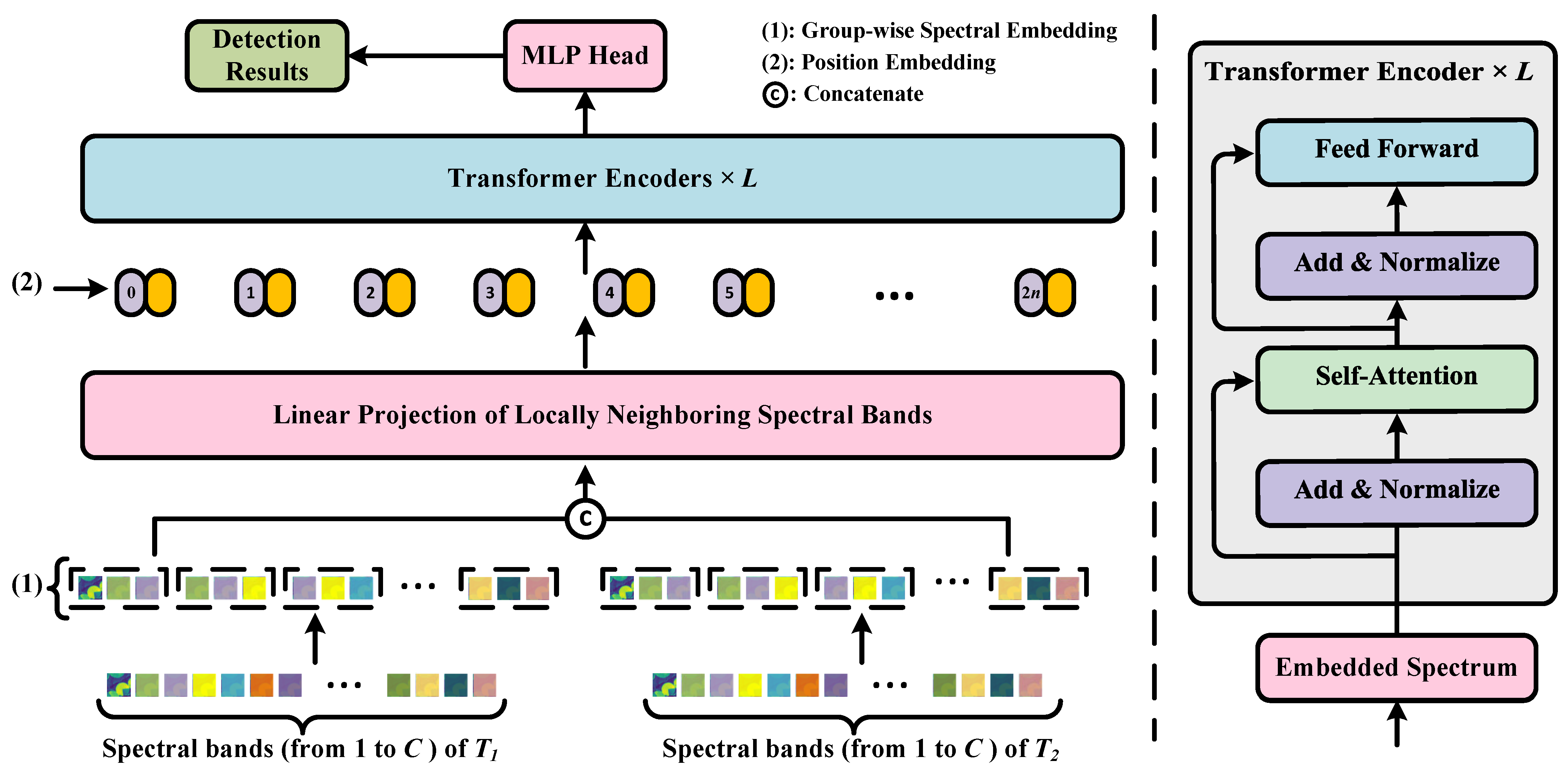
53], and each position on the image corresponds to a temporal variation. This motivates us to explore the representation of hyperspectral pixels and their temporal correlation from a sequential perspective. The Transformer can be adapted to address HSI CD problems by utilizing its long-range modeling ability to characterize the correlation and variability between different spectral bands, as well as the temporal dependency. In this context, we proposed a novel Spectral–Temporal Transformer (STT) for HSI CD. By concatenating the feature embeddings of each image in spectral order, the STT effectively extracts and integrates rich sequence information of the spectrum and time space. With the help of the MHSA mechanism, spectral and temporal information is refined to obtain fused weighted features, which enhances the utilization of temporal information and makes the change features more discriminative.
The main contributions of this paper are summarized as follows:
(1)
The STT is designed with a global spectrum–time-receptive field, enabling the joint capture of spectral information and temporal dependency. By concatenating the feature embeddings in spectral order, the STT learns different representative features between two bands, regardless of spectral or temporal distance, strengthening the utilization of temporal change information.
(2)
We propose a Spectral–Temporal Transformer (STT) for HSI CD, which is the first time the HSI CD task is processed from a completely sequence-based perspective. This enables us to adaptively capture the discriminative sequential properties, e.g., the correlation and variability between different spectral bands and temporal dependency.
The remainder of this paper is organized as follows: Section 2 elaborates on the proposed Spectral–Temporal Transformer (STT) method. Section 3 presents the comparative outcomes of various algorithms on three HSI CD datasets. In Section 4, there is a discussion of the entire paper. Finally, Section 5 provides conclusive remarks.

2. Proposed Method

This section commences with a concise review of the vanilla Transformer architecture, following which we provide a detailed illustration of the structure of our proposed STT method. The overview of our proposed architecture is depicted in Figure 1.

2.1. Vanilla Transformer

The Transformer architecture was originally developed to address NLP tasks, and has demonstrated an exceptional performance by capturing correlations between arbitrary positions throughout the entire sequence. Due to its powerful architecture, Transformer has been explored in CV, resulting in the development of the Vision Transformer (ViT). This novel architecture has demonstrated a superior performance compared to state-of-the-art (SOTA) CNN-based models in a variety of vision-related tasks. This provides new insights, inspiration, and creative opportunities in the field of vision-related tasks. Subsequently, we will explain the elegantly structured architecture of the vanilla Transformer in the following context.
In general, a standard Transformer module contains the following parts: MHSA block, layer normalization (LN), Feed-Forward Network (FFN), and residual connections. The MHSA block can effectively capture various pieces of long-range contextual information by leveraging the SA mechanism. The FFN primarily introduces nonlinearity into the model. The MHSA module conducts multiple parallel attention operations, and subsequently concatenates and projects the resulting outputs to obtain the final values.
M u l t i H e a d = Concat ( head 1 , head 2 , , head h ) W O
where h e a d i is the i-th head of the multi-head attention, W O represents the learned parameters of the linear projection layer, and Concat represents the concatenation operation. Each h e a d i is computed as:
head i = A t t e n t i o n ( Q i , K i , V i )
where Q i , K i , and V i are matrices representing the queries, keys, and values of h e a d i , respectively. The calculation process of Q i , K i , and V i can be described using the following formula:
Q i , K i , V i = E W i Q , E W i K , E W i V
where W Q R d × d / h , W K R d × d / h , and W V R d × d / h are the learned parameters.
The scaled dot-product attention mechanism [37] is generally utilized to calculate the attention score.
A t t e n t i o n ( Q , K , V ) = softmax ( Q K T d k ) V
where d k is the dimension of the keys. The MHSA mechanism employs different attention heads to learn distinct attention patterns that attend to intrinsic features from diverse representation subspaces across varying bands of the concatenated spectral embedding.
The FFN module is utilized further to transform the learned features of all attention heads. This module comprises two linear transformations separated by a Gaussian Error Linear Unit (GELU) activation function.
F F N ( E ) = GELU ( E W 1 ) W 2
The parameters of the linear transformations remain consistent across different positions, but they vary from layer to layer.
In addition, the data are normalized by layer normalization. To handle the challenge of vanishing gradients, residual connections are incorporated into each MHSA and FFN block.

2.2. Spectral–Temporal Transformer

The structure of our STT is presented in Figure 1. To efficiently capture spectral–temporal features, our proposed STT mainly consists of group-wise spectral embedding, linear projection, transformer encoders with an efficient MHSA, and an MLP head for final change detection.

2.2.1. Global Spectral–Temporal Receptive Filed

Spectral sequence and time sequence attributes are crucial for accurate HSI CD, enabling the identification of subtle changes over time and heightening the effectiveness of change detection models. In contrast to using image patches as input, our approach utilizes Group-wise Spectral Embedding (GSE) [54] to leverage the local spectral information. As shown in Figure 2, given an image cube P t R C × h × w with spectral bands of C and spatial size of h × w in T t ( t = 1 , 2 ) HSI, N neighboring bands can be sequentially selected to form local spectral groups with each band as the center.
P G = f ( P ) = [ P 1 , , P Q , , P C ]
where P G R C × N × h × w is the local spectral groups, f ( ) is the function that generates the overlapping groups of bands, and P Q R N × h × w represents the Q-th local spectral group, with the number of neighboring bands being N. Afterwards, the bands in each local spectral group are separately flattened into a sequence to obtain the sequence form P G R C × N h w of the local spectral groups.
Then, the spectral groups of bi-temporal images are concatenated along the spectral dimension and linearly transformed to generate the embedded features.
E G = [ P 1 , G ; P 2 , G ] W
where W R N h w × d and E G R 2 C × d with the feature dimension of d.
Our method involves the concatenation of bi-temporal image data along the spectral dimension to establish a global spectrum–time receptive field. Our proposed STT allows for the simultaneous exploration of both spectral information and temporal dependencies. By concatenating feature embeddings in the spectral dimension, the SST can learn the relationship and difference between any two bands regardless of their spectral and temporal distances, which strengthens the utilization of temporal information. Moreover, this allows for the STT to extract spectral features guided by temporal change information, enhancing the feature discrimination.
Before feeding the embedded features into the transformer encoders, we add position encoding to the sequences.
E = [ C L S ; E G ] + S
where C L S and S = ( s 0 , s 1 , , s C , s 1 , , s C ) denote the class token and positional encoding, respectively. The learned encoding is capable of encoding information related to the absolute or relative position within the spectrum-time domain. This position information can be utilized to direct transformers towards effectively leveraging change information pertaining to the spectrum and time domains.

2.2.2. Efficient Multi-Head Self-Attention Block

The time complexity of the SA mechanism used in transformers is O ( n 2 × d ) , where n is the length of the input sequence and d is the dimension of feature embedding. The computational intensity of this mechanism is due to the dot products and softmax operations, which dictate an individual pairwise computation for each position within the input sequence. The computational cost may be prohibitive for large values of n or d. Researchers have developed several methods to mitigate this issue to reduce the complexity of the self-attention mechanism. Downsampling is an effective technique for reducing the computational complexity of Transformer models by decreasing the resolution of feature maps. However, the HSI consists of numerous bands, with each band carrying important information. Consequently, directly reducing the number of spectral bands may lead to a notable loss of important spectral information. Wang et al. [55] designed an efficient MHSA (EMHSA) block to ease the computational pressure when extracting spectral features using transformers.
The introduced EMHSA block is illustrated in Figure 3b, which provides a detailed overview of its specific components. This block operates on an input sequence X with a sequence length (spectral bands) of n (where n = 2 C ) and a feature-embedding dimension of d. Query (Q) is generated through a linear projection layer, as shown in Equation (3). Before computing the Key (K) and Value (V) components, a 1D convolutional layer is applied to cut down the length of the input sequence.
K i , V i = Conv ( E ) W i K , Conv ( E ) W i V
where Conv denotes the 1D convolutional layer. The sequence length is controlled by setting different stride sizes s called the reduction ratio, which determines the number of overlaps between adjacent spectral bands that the convolutional kernel processes. Following the initial 1D convolutional layer, the quantity of bands (sequence length) is diminished from n to n s = n s . Then, the improved attention distribution with a size of h × n × n s is yielded by the K and V components. Compared to the attention distribution of h × n × n in vanilla self-attention, the reduction in sequence length significantly reduces the computational cost of the attention mechanism. Moreover, a 2D depth-wise convolution layer is utilized to enhance the feature representations. In conclusion, the EMHSA mechanism in this paper can be represented as follows:
E M H S A ( Q , K , V ) = softmax ( DWConv ( Q K T d k ) ) V
where DWConv denotes the 2D depth-wise convolutional layer. As for the remaining operations in EMHSA, they are all the same as the vanilla MHSA mechanism. The computational loads and memory costs are greatly reduced by the efficient self-attention compared to the vanilla MHSA block.
Utilizing the MHSA mechanism, the transform encoders simultaneously focus on varying information across distinct representation subspaces at different bands. This approach effectively leverages the spectral and temporal features within the embedded sequence from a completely sequence-based perspective. This allows us to adaptively capture discriminative sequential properties, such as the correlation and variability between different spectral bands, as well as temporal dependency.
Finally, the C L S token originating from the transformer encoders is fed into the Multi-Layer Perceptron (MLP) Head to produce the final change map. It is notable that the detection result of each C L S token represents whether the central pixel of the image cube has changed.

2.3. Loss Function

The Binary Cross-Entropy (BCE) loss function is widely used in change detection, given its ability to solve binary classification problems. The change detection task involves determining whether each pixel in one image is the same as the corresponding pixel in the other, which can be achieved using binary classification algorithms. Consequently, the BCE loss provides a natural optimization framework for this task.
B C E ( y ^ , y ) = y · log ( y ^ ) + ( 1 y ) · log ( 1 y ^ )
where y ^ is the predicted probability and y is the ground truth label of the given sample.

3. Results

This section begins with an introduction to three HSI CD datasets, along with details on the evaluation measures and implementation. Subsequently, experiments are conducted to assess the efficiency of the proposed Spectral–Temporal Transformer (STT) method.

3.1. Data Description

All the datasets used in this study are collocated by the Earth Observing-1 (EO-1) Hyperion sensor, and the detailed descriptions are shown as follows:

3.1.1. Farmland

The first dataset, Farmland, is shown in Figure 4. It covers a region of farmland located in Yancheng, Jiangsu Province, China. The images in this dataset were acquired on 3 May 2006 and 23 April 2007, respectively. The spatial size of the two images is 420 × 140 pixels. After band removal, the image retains 154 bands for change detection. Notably, the main change in this dataset is the extent of farmland.

3.1.2. Hermiston

The second dataset, Hermiston, is shown in Figure 5. The dataset used in this study includes two HSIs of an irrigated agricultural field located in Hermiston City, OR, USA. The images were acquired on 1 May 2004 and 8 May 2007, respectively, with a resolution of 307 × 241 pixels and comprising 154 spectral bands. In this scene, the main changes are farmland land cover and the edge of the river.

3.1.3. River

The third dataset, River, is displayed in Figure 6. The River dataset was acquired in Jiangsu Province, China, on 3 May 2013 and 31 December 2013, respectively. The dataset contains two HSIs with a size of 463 × 241 pixels and retains 198 spectral bands after noisy band removal. The main type of change is the disappearance of the substance in the river.

3.2. Experimental Settings

3.2.1. Evaluation Metrics

For a quantitative assessment of the three hyperspectral change detection datasets, the Overall Accuracy (OA) and the Kappa coefficient are adopted to evaluate detection performance. The Kappa coefficient can measure whether the model prediction results are consistent with the actual change results. The closer the value is to 1, the better the consistency of the model. In their calculation, four indexes: True Positives (TP), True Negatives (TN), False Positives (FP), and False Negatives (FN), are first counted by the confusion matrix of the detection results. Formally,
O A = T P + T N T P + T N + F N + F P
K a p p a = O A p e 1 p e
p e = ( T P × T N ) + ( T P × T N ) + ( T P × T N ) + ( T P × T N ) ( T P + F P + T N + F N ) 2

3.2.2. Comparative Methods

The following widely used or SOTA methods are compared with the proposed STT approach.
(1)
CVA [7] is a classical method for CD that measures the differences in each band to detect the change regions.
(2)
PCA–CVA [10] employs principal component analysis to maximize the change information, and then CVA is used to detect the change regions.
(3)
TDRD [13] is a tensor-based framework that exploits the high-level semantic information of hyperspectral data by tensor decomposition and reconstruction.
(4)
Untrained CNN (UTCNN) [23] extracts low-level semantic features with the help of CNN’s own structure, which is not trained.
(5)
Recurrent 3D Fully Convolutional Network (Re3FCN) [32] combines a 3D convolutional layer and a ConvLSTM layer to model the temporal change information while maintaining the spatial structure.
(6)
ReCNN [34] combines the strengths of both CNN and RNN to extract fused features from bi-temporal images. To expand the receptive field, dilated convolution is employed.
(7)
Cross-temporal interaction Symmetric Attention Network (CSANet) [49] designs an attention-enhanced symmetric network that employs cross-temporal attention to strengthen the change information obtained from different temporal features.
(8)
SST–Former [52] is a Transformer-based model that sequentially extracts the spatial, spectral, and temporal information of HSIs for CD.

3.2.3. Implementation Details

Our network is implemented using Pytorch on a single NVIDIA GeForce GTX 1660S GPU. We used a batch size of 64 with the Adam optimizer to train the network. The initial learning rate was set to 1 × 10 3 , decaying with a γ factor of 0.9 every ten epochs. Some of the optimal experimental parameters vary on different datasets, so we summarize them in Table 1. The dimensionality of the spectrum embeddings is 64.

3.3. Experimental Results

3.3.1. Results of Farmland Dataset

Figure 7 presents the visual observations of the Farmland dataset. Obviously, the dividing boundaries between farmlands at the top of the images are falsely detected as changed regions for CVA. Though PCA–CVA, TDRD, and UTCNN have better visual observations, they still have many missed detections in the lower middle area. Moreover, the boundaries of the changed regions are glued together for TDRD and UTCNN. Because of the difficulty extracting discriminative features without labeled samples, these unsupervised methods tend to have a lower accuracy than other methods. The supervised methods have fewer misclassified pixels, and our proposed method even maintains the change region’s edges well. As reported in Table 2, all the unsupervised methods yield OA lower than 90%, while the supervised methods achieve higher OA and Kappa values. Compared to CVA, PCA–CVA reduces data redundancy and noise, TDRD increases the utilization of spatial and temporal information, and UTCNN extracts deep features, which makes their performance better than CVA. It is notable that although the OA of PCA–CVA, TDRD, and UTCNN are similar, the Kappa of PCA–CVA is smaller than the latter two, indicating poor consistency. The ReCNN method, which solely employs 2D convolutions to extract spatial features, exhibits the poorest performance among all supervised methods. While Re3FCN enhances the utilization of spatial and spectral information through 3D convolutions, CSANet employs attention mechanisms to improve the use of temporal information, resulting in a superior performance. Although SST–Former incorporates global modeling capabilities through the Transformer, it is still based on the Siamese network, so it does not achieve satisfactory results. Its Kappa does not exceed 0.90, making it significantly worse than supervised methods other than ReCNN. Our proposed STT has the best detection performance, with an OA of 96.56% and Kappa of 0.9209, showing that the STT with the global spectrum–time receptive-field extracts joint weighted features, improving the utilization of temporal change information.

3.3.2. Results of Hermiston Dataset

The detection results on the Hermiston dataset are displayed in Figure 8 and Table 3. The major changes detected in this dataset occurred in the farmland areas and the edge of the river. As shown in Figure 8a–d, many changed regions cannot be detected by the unsupervised methods. PCA–CVA performs slightly worse than CVA, with OA and Kappa lower by 0.47% and 0.0185, respectively, which also reflects the lack of robustness of these traditional methods. UTCNN is a neural network-based approach, but it scores the worst among all the compared methods because it is not trained with any prior information. Although the visual performance of Re3FCN and ReCNN is very close, since they are both based on CNN and RNN, ReCNN is significantly better than Re3FCN on OA and Kappa. CSANet cannot detect the river’s edge, but its quantitative performance is relatively ideal, 0.52% higher than ReCNN in OA and 0.0164 in Kappa. This also confirms the importance of attention mechanisms. SST–Former obtains the second-best performance because it fully exploits spectral information but lacks the interaction of temporal information during feature extraction. Our proposed STT method achieves the best results among the compared methods, with the fewest missed or false detections. This is particularly evident in the upper right area of the hyperspectral images, where the changes are more complex and difficult to detect. By adaptively fusing the discriminative information of different bands, the STT achieves an OA of 96.91% and a Kappa of 0.9101, respectively.

3.3.3. Results of River Dataset

Figure 9 and Table 4 detail the comparison results for the River dataset. Based on a thorough analysis of all the visual and quantitative results, it can be concluded that the STT exhibits the best detection results among all the tested approaches. Specifically, the results obtained by UTCNN show that the changing regions are almost entirely connected, yielding the worst OA and Kappa. This also reflects the inadequacy of untrained neural networks in extracting discriminative features. PCA–CVA yields a higher OA and Kappa than CVA; because of dimension reduction, PCA–CVA removes more redundant information and noise. While the OA of PCA–CVA is lower than that of TDRD, its Kappa is slightly higher, indicating that PCA–CVA exhibits better consistency than TDRD. Among all unsupervised methods, TDRD yields the best results, even surpassing the performance of some supervised approaches, e.g., its OA and Kappa exceed ReCNN by 0.27% and 0.0346, respectively. These findings suggest that the River dataset has more complicated scenes than the Farmland and Hermiston datasets. Therefore, at the current ratio of samples, ReCNN and CSANet struggle to fit the training data well and exhibit poor learning capabilities. SST–Former produces the second-best result among all results but still lags behind our proposed method by a large margin, and its OA and Kappa are 0.99% and 0.0633 lower than ours, respectively. Our proposed STT earns the best results on all evaluation metrics, including an OA of 97.74% and a Kappa coefficient of 0.8493. The results indicate that our proposed STT is better-suited to mining the spectral sequence properties of hyperspectral data on datasets with more spectral bands.

3.4. Parameter Sensitivity Analysis

3.4.1. The Number of Neighboring Bands

The number of neighboring bands determines how many local spectral embeddings are utilized to facilitate feature extraction. The model’s performance is analyzed through verification experiments, wherein the number of neighboring bands varies between 1 and 9. As observed in Table 5, an increased number of neighboring bands proves advantageous in excavating subtle spectral discrepancies, thus significantly improving the detection accuracy. However, too many neighbors will introduce more noise and redundant information, causing the model to deteriorate. The optimal scaling must ensure adequate spectral texture while simultaneously avoiding excessive noise interference. The results indicate that the optimal model performance on the Farmland and Hermiston datasets is obtained when the number of neighboring bands is 5. Similarly, although the best results on the River dataset are achieved when the number of neighboring bands is 7, the difference in performance compared to when the number of neighboring bands is 5 is not significant. Moreover, as selecting the former significantly increases memory consumption, opting for 5 neighboring bands is a more cost-effective decision.

3.4.2. The Reduction Ratio of Efficient Self-Attention Design

Determining an appropriate ratio s is very important to strike a balance between model accuracy and computational efficiency. We investigate the effectiveness of the EMHSA block and the suitable choices for the reduction ratio for the spectral–temporal transformer. As presented in Figure 10, the structure with the EMHSA block outperforms vanilla MHSA in the STT. This can be attributed to the 1D convolution inthe EMHSA block, which enhances the utilization of local information while simultaneously mitigating redundancy amidst different bands of hyperspectral data. Then, Figure 10 delves deeper into the investigation of the requirement and reduction ratio for diminishing the sequence length. Regarding the Farmland and Hermiston datasets, the optimal detection outcomes are attained when s = 2 , surpassing the vanilla Transformer’s OA and Kappa, respectively. This can be attributed to the efficacy of the EMHSA mechanism in eliminating band redundancy and noise. As for the River dataset, both s = 2 and s = 4 yield satisfactory results. This can be explained by the fact that the River dataset has a larger number of bands, resulting in increased redundancy. Nonetheless, while the above results corroborate the efficacy of sequence length reductions, an excessively large s may lead to diminished model representation abilities and, consequently, worse change detection results.

3.4.3. The Number of Training Samples

To comprehensively analyze the impact of varied training sample sizes on detection performance, we employ several supervised methods to test the detection results on the Hermiston and River datasets. Specifically, we train Re3FCN, ReCNN, CSANet, SST–Former, and STT models using labeled samples of 1%, 3%, 5%, 10%, and 20% in strata while keeping the samples consistent across all the methods. As presented in Figure 11, our proposed STT outperforms other methods across various training data sizes, only slightly lower than SST–Former when the training ratio is 1% on the River dataset. The reason is that the proposed STT with a global spectrum–time receptive field takes advantage of the temporal dependency and adaptively fuses the discriminative information of different bands, capable of learning the subtle change features. It is notable that the OA of the other CNN-based methods decreases significantly as the training sample size reduces, while the transformer-based methods have better robustness. However, in contrast to the STT, the performance of SST–Former does not exhibit notable improvements as the ratio of training data increases. This observation highlights that our proposed STT exhibits a superior generalization performance, as it is not merely memorizing the examples but learning the general patterns.

3.5. Ablation Experiments

To illustrate the effectiveness of group-wise spectral embedding and efficient multihead self-attention, we perform ablation experiments on three datasets.

3.5.1. Group-Wise Spectral Embedding

GSE allows for us to leverage the local spectral information. As shown in Table 6, Model (1) achieves the worst performance for all the datasets, especially the Farmland dataset. The OA and Kappa of Model (2) with GSE are improved compared to Model (1). Model (4) further improves the detection performance with the addition of GSE to Model (3) and achieves the best performance. This is because GSE is able to extract local spectral features, thus improving the accuracy of CD.

3.5.2. Efficient Multi-Head Self-Attention

The EMHSA block is able to reduce the redundancy of spectral embedding and improve computational efficiency. The experimental results are presented in Table 6. Compared with Model (1), Model (3) significantly improved OA and Kappa on three datasets after changing from the vanilla MHSA to the EMHSA. Moreover, the best performance was produced by Model (4), which was obtained after the addition of EMHSA to Model (2). This indicates that EMHSA is able to remove spectral redundancy and noise, enhancing the performance of CD.

4. Discussion

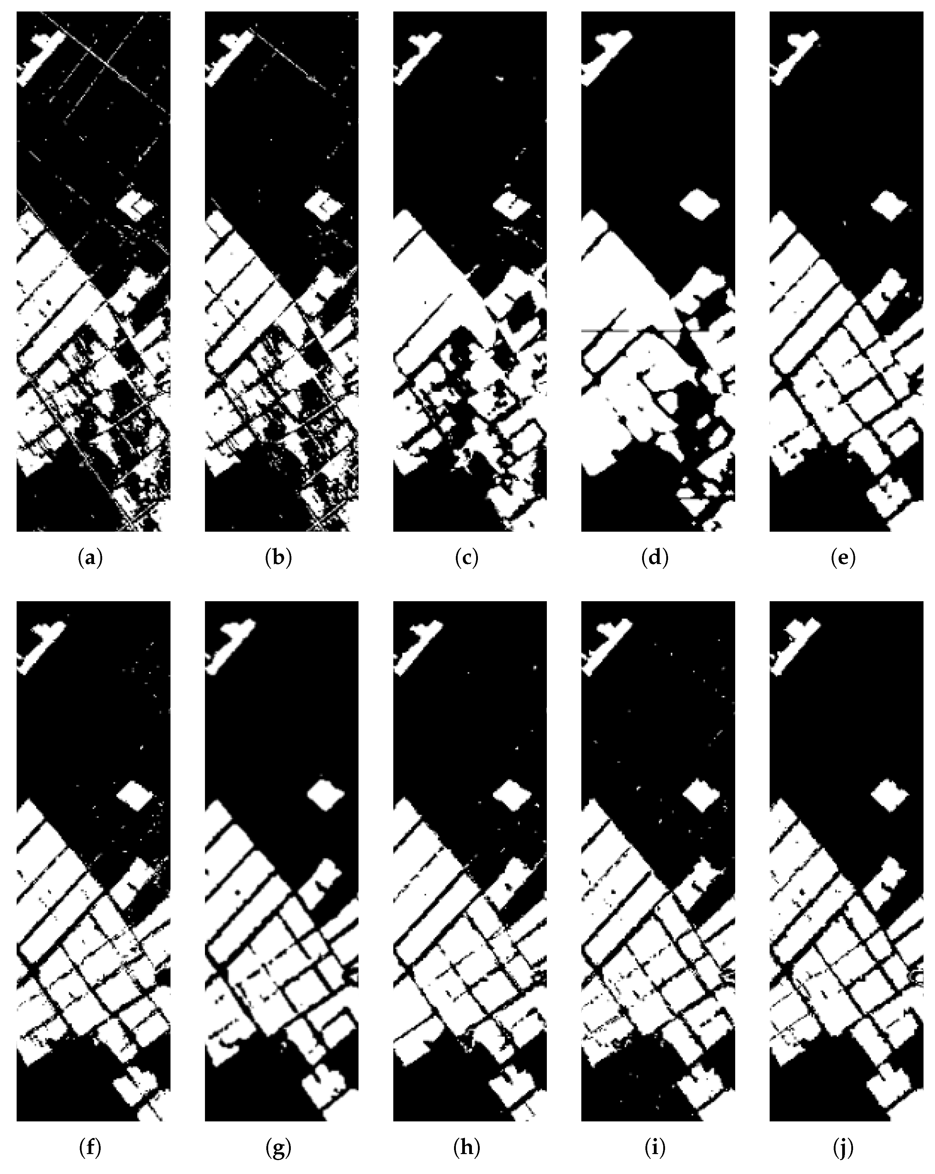
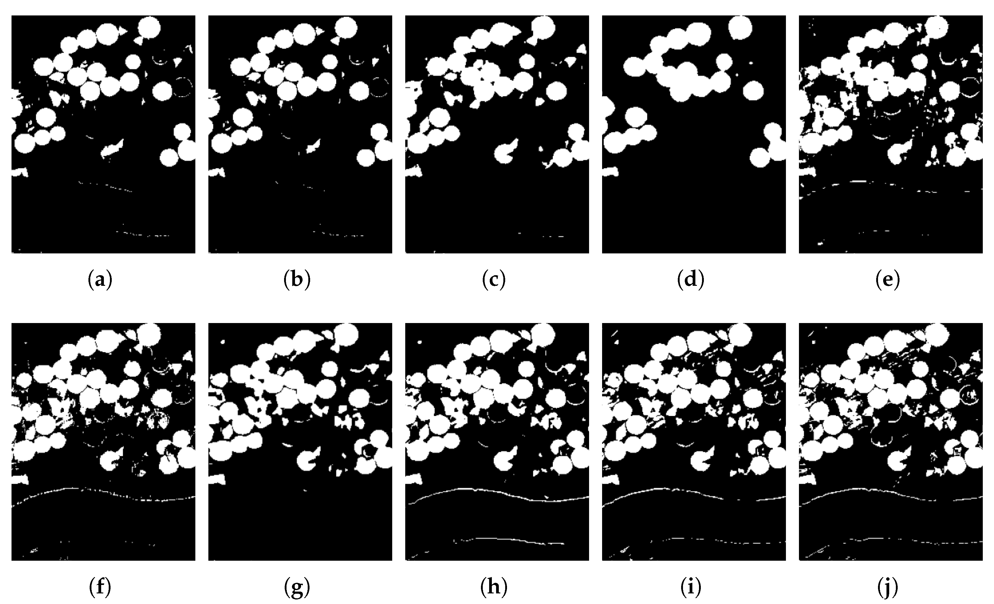
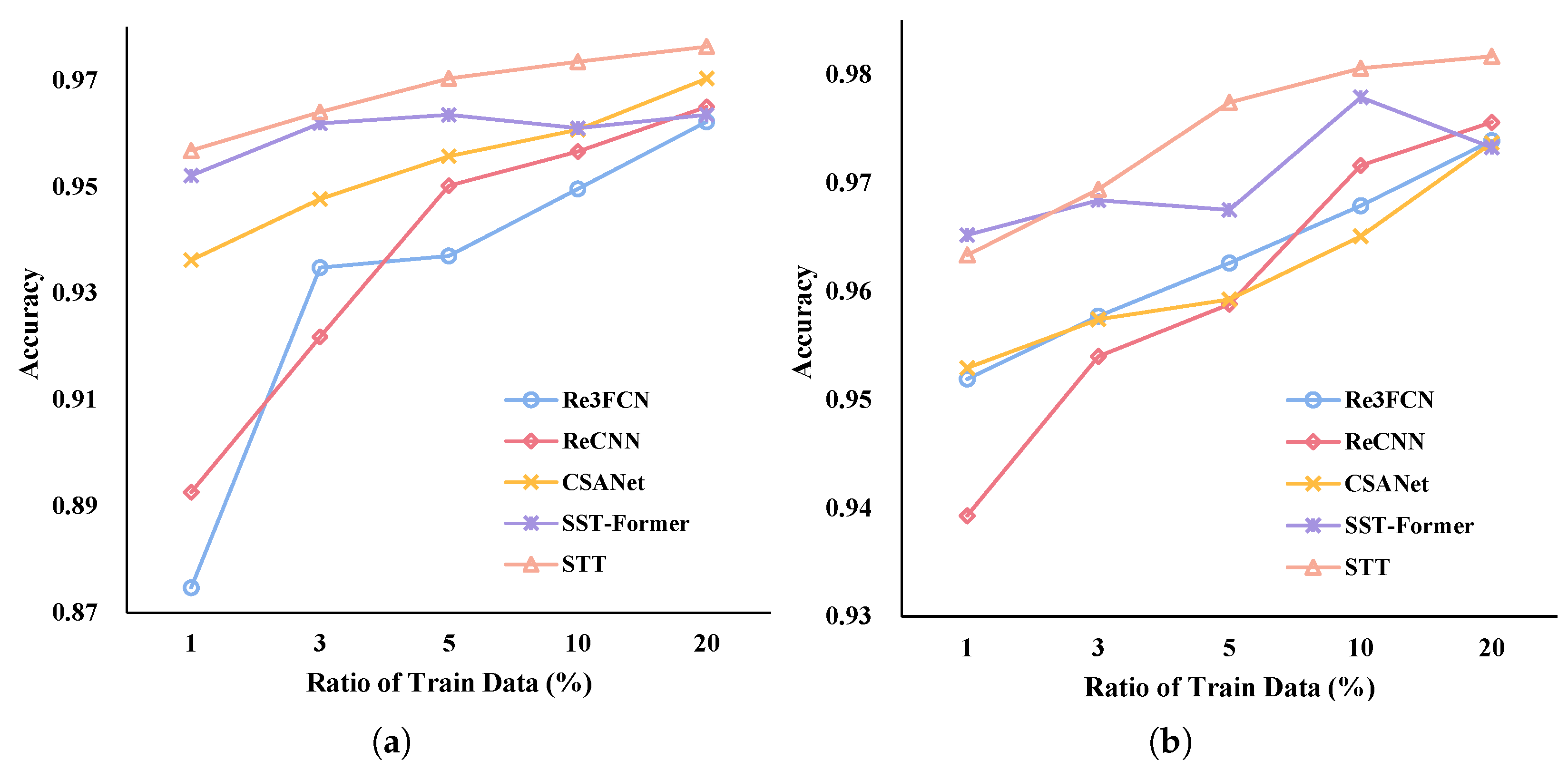
To verify the effectiveness of the proposed Spectral–Temporal Transformer, we perform a series of experiments with varying parameters on three widely used hyperspectral image change detection datasets and compare the results with those obtained from eight other methods: CVA, PCA–CVA, TDRD, UTCNN, Re3FCN, ReCNN, CSANet, and SST–Former.
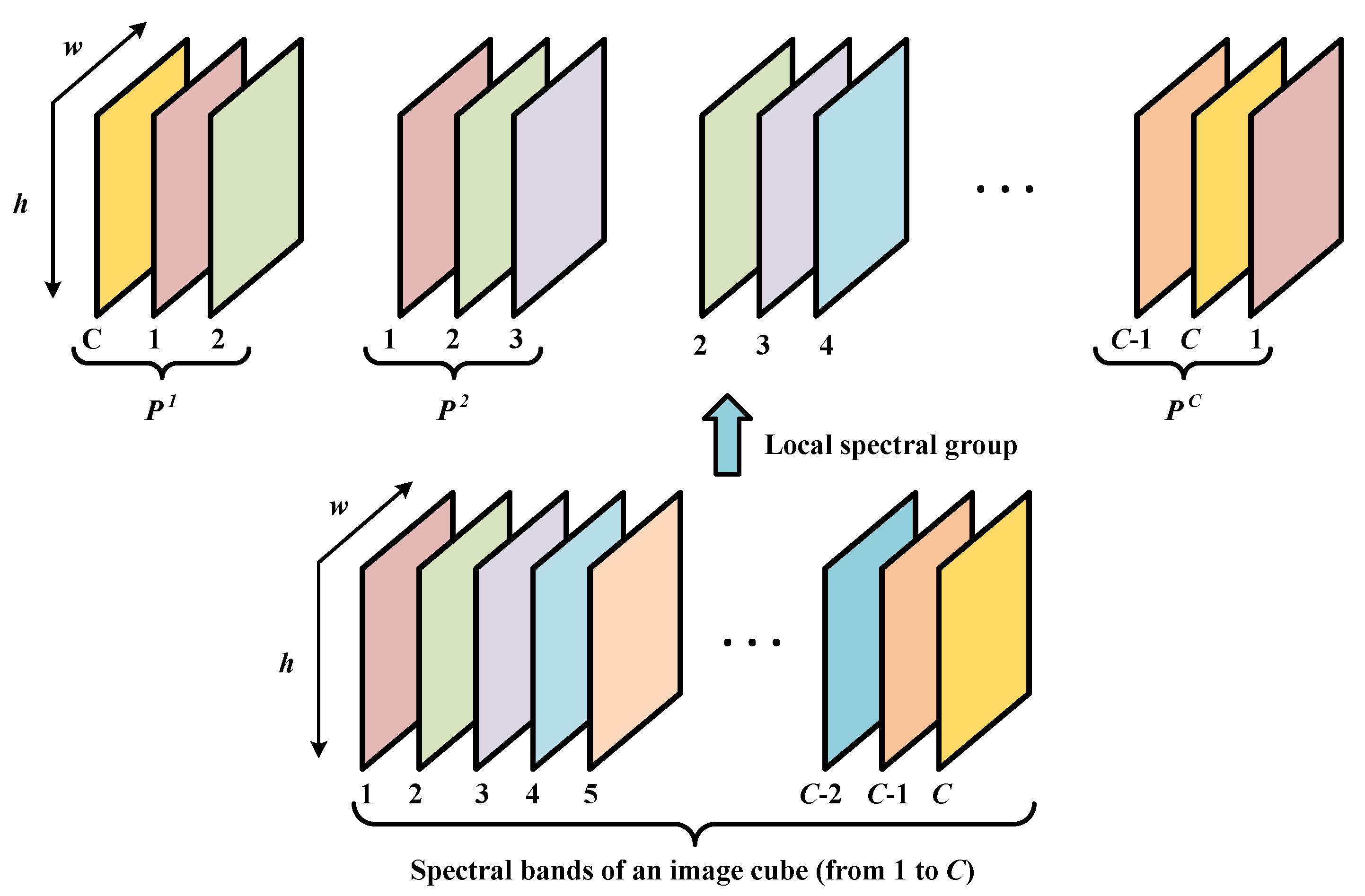
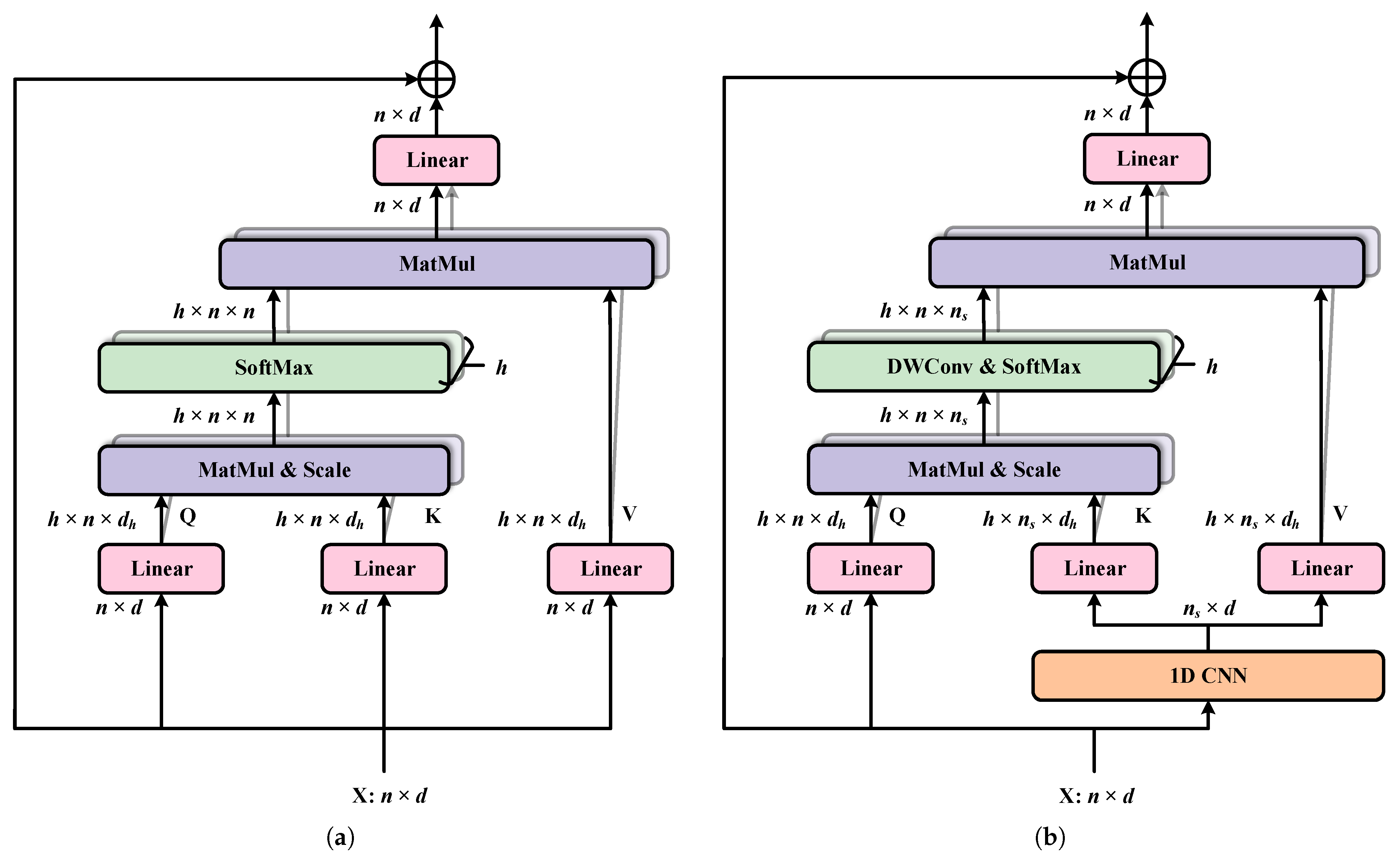
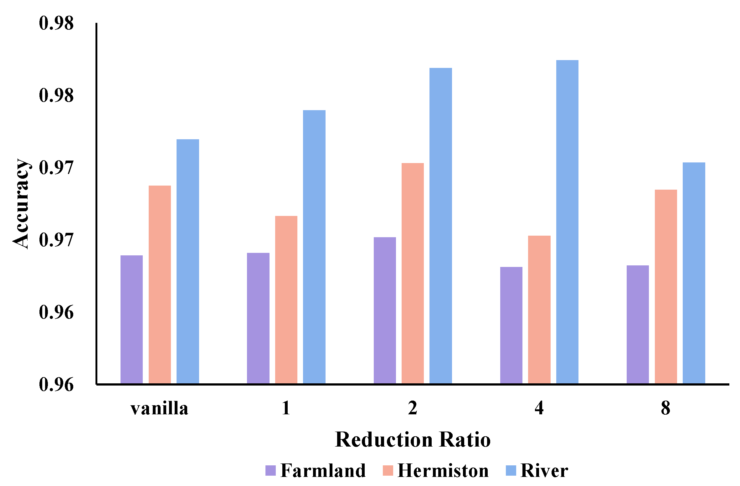
Aiming to fully explore the discriminative sequential properties of bi-temporal HSIs, e.g., the correlation and variability between different spectral bands, and temporal dependency, we construct a global spectrum–time-receptive field based on Transformer in the proposed STT method. Group-wise band embedding and efficient multi-head self-attention are employed to strengthen the use of local band information and improve computation efficiency, respectively.
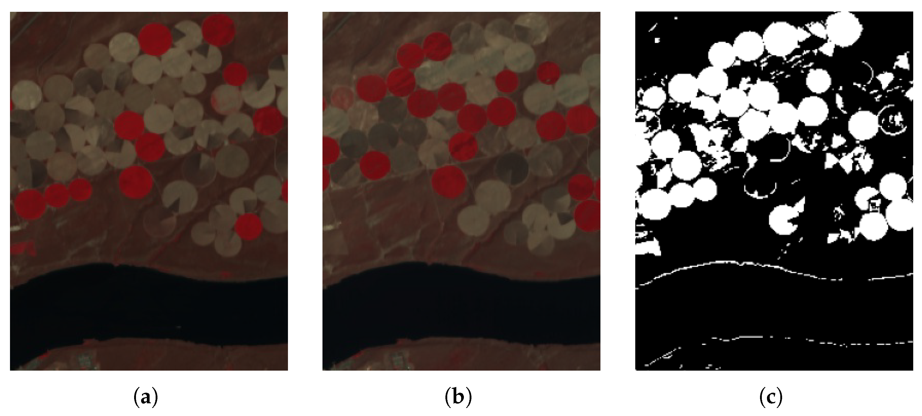
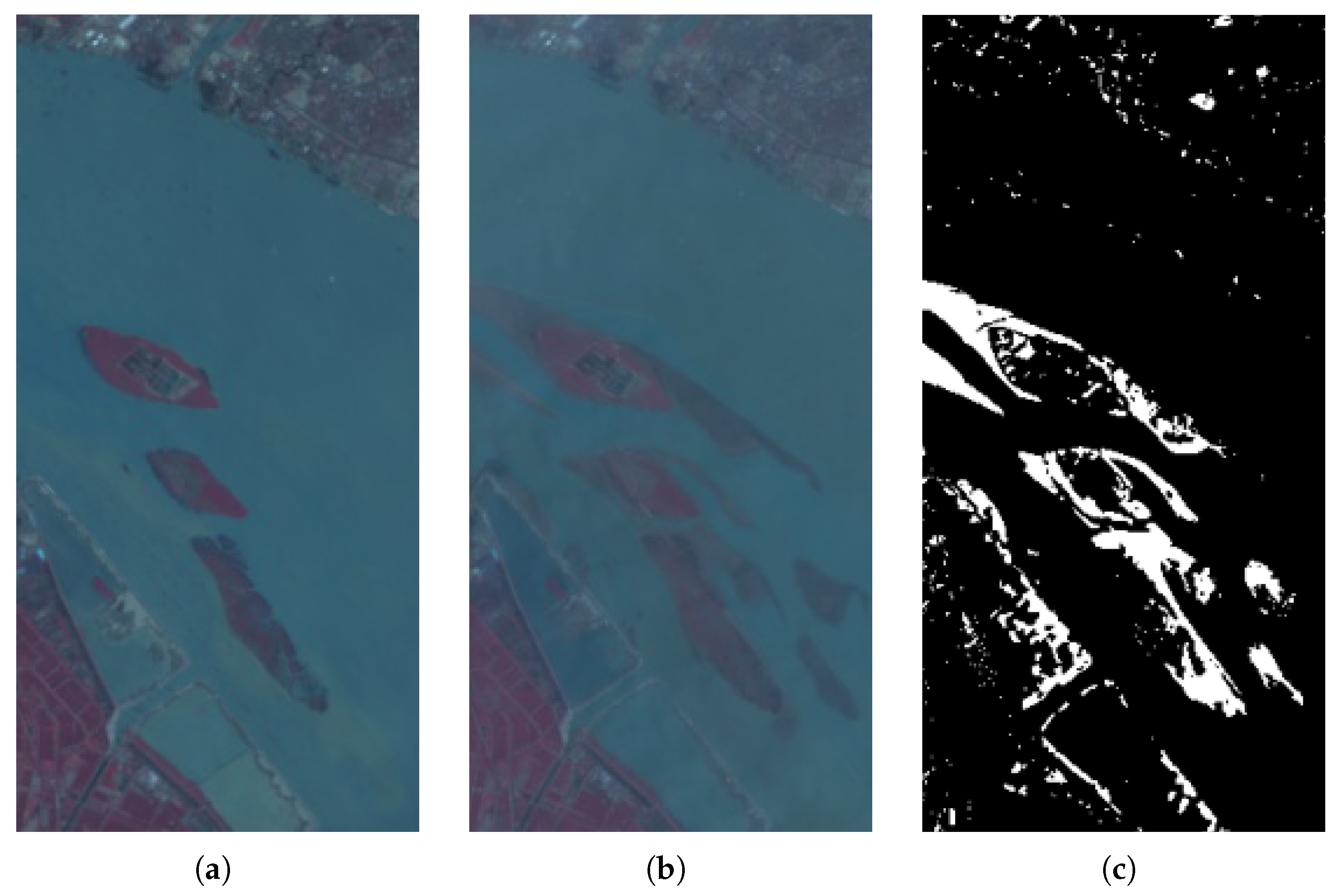
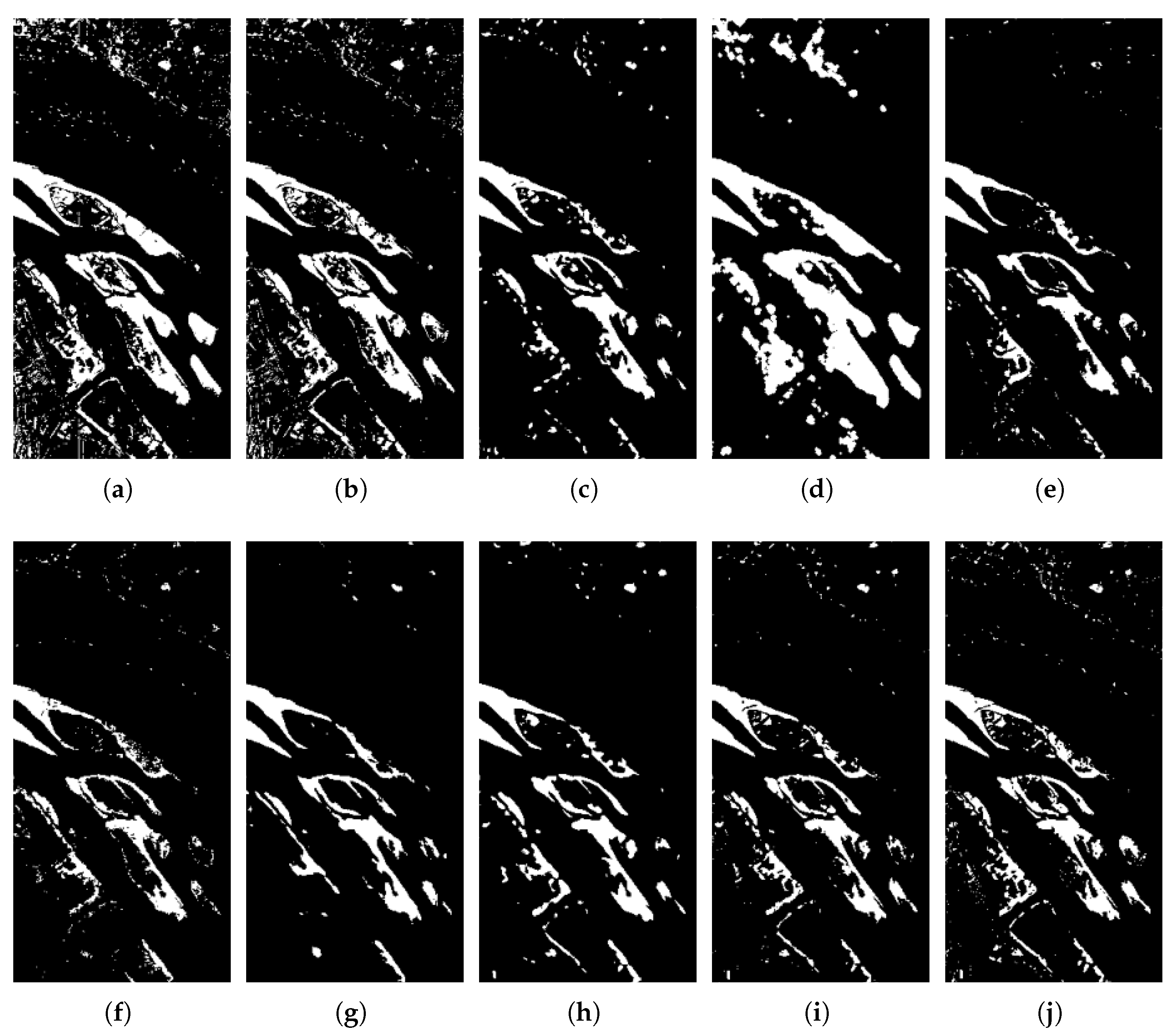
We utilize OA and Kappa scores as objective evaluation measures to comprehensively assess the performance of the proposed methods in HSI CD, enabling a rigorous comparison of different approaches. As presented in Figure 7, Figure 8 and 
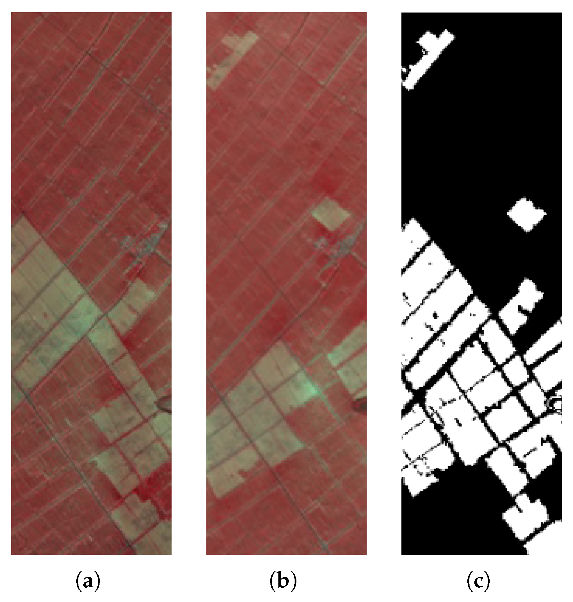
Figure 9, our proposed method exhibits the best visual performance. As presented in Table 4, Table 5 and Table 6, the proposed method offers superior detection abilities compared to other algorithms. In particular, on the River dataset with more bands, our proposed method has a significant lead thanks to the full exploitation of the sequence properties of HSIs. Based on the analysis of the detection results, we can conclude that the STT has an excellent detection performance compared to the above methods. These results highlight the effectiveness and potential of STT in addressing the HSI CD task, providing valuable insights into the performance of different methods.
While our algorithm demonstrates a superior detection performance, it is important to note that several limitations still exist, which must be addressed in future research. The incorporation of spatial information is essential in remote sensing image processing. Although we can obtain spatial information from image patches, the spatial structure is lost in the subsequent feature-extraction process. This highlights the need for further research to address the challenge of preserving spatial information.

5. Conclusions

This study introduced a novel Transformer-based method for HSI CD called the Spectral–Temporal Transformer (STT). The proposed STT simultaneously considers both the intrinsic sequential structure of hyperspectral data and time sequence information. This is the first time the HSI CD task has been processed from a completely sequential perspective. The experimental results for three HSI datasets demonstrate the competitive performance of our proposed method for HSI CD. Further, we find that improving the utilization of the local information of the spectrum and reducing the redundancy between bands are beneficial to improving the performance of CD through parametric analysis and ablation experiments.
Although our proposed method improves the accuracy of CD by extracting joint spectral–temporal information, it lacks the mining of spatial information. Therefore, in future work, CNNs or other techniques that help extract spatial information will be introduced to further improve the performance of CD.

Author Contributions

Research design and results analysis, J.D.; advice providing, review and funding acquisition, X.L. All authors have reviewed and approved the final version of the manuscript for publication.

Funding

This work was funded in part by the National Nature Science Foundation of China under Grant 62171404.

Data Availability Statement

The Farmland and Hermiston Datasets are available at https://rslab.ut.ac.ir/data, accessed on 10 May 2023 and River Dataset at http://crabwq.github.io, accessed on 10 May 2023.

Conflicts of Interest

The authors declare no conflict of interest.

References

  1. Borana, S.; Yadav, S.; Parihar, S. Hyperspectral Data Analysis for Arid Vegetation Species: Smart & Sustainable Growth. In Proceedings of the 2019 International Conference on Computing, Communication, and Intelligent Systems (ICCCIS), Greater Noida, India, 18–19 October 2019; pp. 495–500. [Google Scholar]
  2. Chang, S.; Kopp, M.; Ghamisi, P. Multiview Subspace Learning for Hyperspectral Anomalous Change Detection. IEEE Trans. Geosci. Remote Sens. 2022, 60, 1–12. [Google Scholar] [CrossRef]
  3. Rokni, K.; Ahmad, A.; Selamat, A.; Hazini, S. Feature Extraction and Change Detection Using Multitemporal Landsat Imagery. Remote Sens. 2014, 6, 4173–4189. [Google Scholar] [CrossRef] [Green Version]
  4. Hu, M.; Wu, C.; Zhang, L.; Du, B. Hyperspectral Anomaly Change Detection Based on Autoencoder. IEEE J. Sel. Top. Appl. Earth Observ. Remote Sens. 2021, 14, 3750–3762. [Google Scholar] [CrossRef]
  5. Bruzzone, L.; Prieto, D.F. Automatic Analysis of the Difference Image for Unsupervised Change Detection. IEEE Trans. Geosci. Remote Sens. 2000, 38, 1171–1182. [Google Scholar] [CrossRef] [Green Version]
  6. Bazi, Y.; Bruzzone, L.; Melgani, F. An Unsupervised Approach Based on the Generalized Gaussian Model to Automatic Change Detection in Multitemporal SAR Images. IEEE Trans. Geosci. Remote Sens. 2005, 43, 874–887. [Google Scholar] [CrossRef] [Green Version]
  7. Bovolo, F.; Bruzzone, L. A Theoretical Framework for Unsupervised Change Detection Based on Change Vector Analysis in the Polar Domain. IEEE Trans. Geosci. Remote Sens. 2007, 45, 218–236. [Google Scholar] [CrossRef] [Green Version]
  8. Saha, S.; Bovolo, F.; Bruzzone, L. Unsupervised Deep Change Vector Analysis for Multiple-Change Detection in VHR Images. IEEE Trans. Geosci. Remote Sens. 2019, 57, 3677–3693. [Google Scholar] [CrossRef]
  9. Thonfeld, F.; Feilhauer, H.; Braun, M.; Menz, G.R. Change Vector Analysis (RCVA) for Multi-Sensor Very High Resolution Optical Satellite Data. Int. J. Appl. Earth Obs. Geoinf. 2016, 50, 131–140. [Google Scholar] [CrossRef]
  10. Baisantry, M.; Negi, D.; Manocha, O. Change Vector Analysis Using Enhanced PCA and Inverse Triangular Function-based Thresholding. Def. Sci. J. 2012, 62, 236–242. [Google Scholar] [CrossRef]
  11. Nielsen, A.A.; Conradsen, K.; Simpson, J.J. Multivariate Alteration Detection (MAD) and MAF Postprocessing in Multispectral, Bitemporal Image Data: New Approaches to Change Detection Studies. Remote Sens. Environ. 1998, 64, 1–19. [Google Scholar] [CrossRef] [Green Version]
  12. Nielsen, A.A. The Regularized Iteratively Reweighted MAD Method for Change Detection in Multi- and Hyperspectral Data. IEEE Trans. Image Process. 2007, 16, 463–478. [Google Scholar] [CrossRef] [PubMed] [Green Version]
  13. Hou, Z.; Li, W.; Tao, R.; Du, Q. Three-Order Tucker Decomposition and Reconstruction Detector for Unsupervised Hyperspectral Change Detection. IEEE J. Sel. Top. Appl. Earth Observ. Remote Sens. 2021, 14, 6194–6205. [Google Scholar] [CrossRef]
  14. Bovolo, F.; Bruzzone, L.; Marconcini, M. A Novel Approach to Unsupervised Change Detection Based on a Semisupervised SVM and a Similarity Measure. IEEE Trans. Geosci. Remote Sens. 2008, 46, 2070–2082. [Google Scholar] [CrossRef] [Green Version]
  15. Demir, B.; Bovolo, F.; Bruzzone, L. Detection of Land-Cover Transitions in Multitemporal Remote Sensing Images with Active-Learning-Based Compound Classification. IEEE Trans. Geosci. Remote Sens. 2012, 50, 1930–1941. [Google Scholar] [CrossRef]
  16. Krizhevsky, A.; Sutskever, I.; Hinton, G.E. Imagenet Classification with Deep Convolutional Neural Networks. Commun. ACM 2017, 60, 84–90. [Google Scholar] [CrossRef] [Green Version]
  17. He, K.; Zhang, X.; Ren, S.; Sun, J. Deep Residual Learning for Image Recognition. In Proceedings of the IEEE Conference on Computer Vision and Pattern Recognition, Las Vegas, NV, USA, 27–30 June 2016. [Google Scholar]
  18. Tan, M.; Le, Q. EfficientNet: Rethinking Model Scaling for Convolutional Neural Networks. In Proceedings of the International Conference on Machine Learning, Long Beach, CA, USA, 9–15 June 2019. [Google Scholar]
  19. Zhan, T.; Gong, M.; Jiang, X.; Zhao, W. Transfer Learning-Based Bilinear Convolutional Networks for Unsupervised Change Detection. IEEE Geosci. Remote Sens. Lett. 2022, 19, 1–5. [Google Scholar] [CrossRef]
  20. Ling, J.; Hu, L.; Cheng, L.; Chen, M.; Yang, X. IRA-MRSNet: A Network Model for Change Detection in High-Resolution Remote Sensing Images. Remote Sens. 2022, 14, 5598. [Google Scholar] [CrossRef]
  21. Lei, T.; Geng, X.; Ning, H.; Lv, Z.; Gong, M.; Jin, Y.; Nandi, A.K. Ultra-Lightweight Spatial-Spectral Feature Cooperation Network for Change Detection in Remote Sensing Images. IEEE Trans. Geosci. Remote Sens. 2023, 61, 1. [Google Scholar]
  22. Wang, Q.; Yuan, Z.; Du, Q.; Li, X. GETNET: A General End-to-End 2-D CNN Framework for Hyperspectral Image Change Detection. IEEE Trans. Geosci. Remote Sens. 2019, 57, 3–13. [Google Scholar] [CrossRef] [Green Version]
  23. Saha, S.; Kondmann, L.; Song, Q.; Zhu, X. Change Detection in Hyperdimensional Images Using Untrained Models. IEEE J. Sel. Top. Appl. Earth Observ. Remote Sens. 2021, 14, 11029–11041. [Google Scholar] [CrossRef]
  24. Zhan, T.; Song, B. TDSSC: A Three-Directions Spectral–Spatial Convolution Neural Network for Hyperspectral Image Change Detection. IEEE J. Sel. Top. Appl. Earth Observ. Remote Sens. 2021, 14, 377–388. [Google Scholar] [CrossRef]
  25. Song, B.; Tang, Y.; Zhan, T.; Wu, Z. BRCN-ERN: A Bidirectional Reconstruction Coding Network and Enhanced Residual Network for Hyperspectral Change Detection. IEEE Geosci. Remote Sens. Lett. 2022, 19, 1–5. [Google Scholar] [CrossRef]
  26. Zhan, T.; Song, B.; Xu, Y.; Wan, M.; Wang, X.; Yang, G.; Wu, Z. SSCNN-S: A Spectral-Spatial Convolution Neural Network with Siamese Architecture for Change Detection. Remote Sens. 2021, 13, 895. [Google Scholar] [CrossRef]
  27. Ou, X.; Liu, L.; Tu, B.; Zhang, G.; Xu, Z. A CNN Framework with Slow-Fast Band Selection and Feature Fusion Grouping for Hyperspectral Image Change Detection. IEEE Trans. Geosci. Remote Sens. 2022, 60, 1–16. [Google Scholar] [CrossRef]
  28. Wang, L.; Wang, L.; Wang, Q.; Bruzzone, L. RSCNet: A Residual Self-Calibrated Network for Hyperspectral Image Change Detection. IEEE Trans. Geosci. Remote Sens. 2022, 60, 1–17. [Google Scholar] [CrossRef]
  29. Zhao, C.; Cheng, H.; Feng, S. A Spectral–Spatial Change Detection Method Based on Simplified 3-D Convolutional Autoencoder for Multitemporal Hyperspectral Images. IEEE Geosci. Remote Sens. Lett. 2022, 19, 1–5. [Google Scholar] [CrossRef]
  30. Seydi, S.; Shah-Hosseini, R.; Amani, M. A Multi-Dimensional Deep Siamese Network for Land Cover Change Detection in Bi-Temporal Hyperspectral Imagery. Sustainability 2022, 14, 12597. [Google Scholar] [CrossRef]
  31. Lyu, H.; Lu, H.; Mou, L. Learning a Transferable Change Rule from a Recurrent Neural Network for Land Cover Change Detection. Remote Sens. 2016, 8, 506. [Google Scholar] [CrossRef] [Green Version]
  32. Song, A.; Choi, J.; Han, Y.; Kim, Y. Change Detection in Hyperspectral Images Using Recurrent 3D Fully Convolutional Networks. Remote Sens. 2018, 10, 1827. [Google Scholar] [CrossRef] [Green Version]
  33. Shi, C.; Zhang, Z.; Zhang, W.; Zhang, C.; Xu, Q. Learning Multiscale Temporal–Spatial–Spectral Features via a Multipath Convolutional LSTM Neural Network for Change Detection with Hyperspectral Images. IEEE Trans. Geosci. Remote Sens. 2022, 60, 1–16. [Google Scholar] [CrossRef]
  34. Mou, L.; Bruzzone, L.; Zhu, X. Learning Spectral-Spatial-Temporal Features via a Recurrent Convolutional Neural Network for Change Detection in Multispectral Imagery. IEEE Trans. Geosci. Remote Sens. 2019, 57, 924–935. [Google Scholar] [CrossRef] [Green Version]
  35. Bahdanau, D.; Cho, K.; Bengio, Y. Neural Machine Translation by Jointly Learning to Align and Translate. arXiv 2014, arXiv:1409.0473. [Google Scholar]
  36. Seo, M.; Kembhavi, A.; Farhadi, A.; Hajishirzi, H. Bidirectional Attention Flow for Machine Comprehension. arXiv 2016, arXiv:1611.01603. [Google Scholar]
  37. Vaswani, A.; Shazeer, N.; Parmar, N.; Uszkoreit, J.; Jones, L.; Gomez, A.N.; Kaiser, L.; Polosukhin, I. Attention Is All You Need. In Proceedings of the Advances in Neural Information Processing Systems, Long Beach, CA, USA, 4–9 December 2017. [Google Scholar]
  38. Xu, K.; Ba, J.; Kiros, R.; Cho, K.; Courville, A.; Salakhudinov, R.; Zemel, R.; Bengio, Y. Show, Attend and Tell: Neural Image Caption Generation with Visual Attention. In Proceedings of the International Conference on Machine Learning, Lille, France, 7–9 July 2015. [Google Scholar]
  39. Woo, S.; Park, J.; Lee, J.; Kweon, I.S. CBAM: Convolutional Block Attention Module. In Proceedings of the Computer Vision—ECCV, Munich, Germany, 8–14 September 2018. [Google Scholar]
  40. Hu, J.; Shen, L.; Sun, G. Squeeze-and-Excitation Networks. In Proceedings of the IEEE Conference on Computer Vision and Pattern Recognition, Salt Lake City, UT, USA, 18–24 June 2018. [Google Scholar]
  41. Dosovitskiy, A.; Beyer, L.; Kolesnikov, A.; Weissenborn, D.; Zhai, X.; Unterthiner, T.; Dehghani, M.; Minderer, M.; Heigold, G.; Gelly, S.; et al. An Image Is Worth 16×16 Words: Transformers for Image Recognition at Scale. arXiv 2021, arXiv:2010.11929. [Google Scholar]
  42. Gong, M.; Jiang, F.; Qin, A.K.; Liu, T.; Zhan, T.; Lu, D.; Zheng, H.; Zhang, M. A Spectral and Spatial Attention Network for Change Detection in Hyperspectral Images. IEEE Trans. Geosci. Remote Sens. 2021, 60, 1. [Google Scholar] [CrossRef]
  43. Wang, Z.; Jiang, F.; Liu, T.; Xie, F.; Li, P. Attention-Based Spatial and Spectral Network with PCA-Guided Self-Supervised Feature Extraction for Change Detection in Hyperspectral Images. Remote Sens. 2021, 13, 4927. [Google Scholar] [CrossRef]
  44. Huang, Y.; Zhang, L.; Huang, C.; Qi, W.; Song, R. Parallel Spectral–Spatial Attention Network with Feature Redistribution Loss for Hyperspectral Change Detection. Remote Sens. 2022, 15, 246. [Google Scholar] [CrossRef]
  45. Qu, J.; Hou, S.; Dong, W.; Li, Y.; Xie, W. A Multilevel Encoder–Decoder Attention Network for Change Detection in Hyperspectral Images. IEEE Trans. Geosci. Remote Sens. 2022, 60, 1–13. [Google Scholar] [CrossRef]
  46. Wang, L.; Wang, L.; Wang, Q.; Atkinson, P.M. SSA-SiamNet: Spectral–Spatial-Wise Attention-Based Siamese Network for Hyperspectral Image Change Detection. IEEE Trans. Geosci. Remote Sens. 2022, 60, 1–18. [Google Scholar] [CrossRef]
  47. Luo, F.; Zhou, T.; Liu, J.; Guo, T.; Gong, X.; Ren, J. Multi-Scale Diff-changed Feature Fusion Network for Hyperspectral Image Change Detection. IEEE Trans. Geosci. Remote Sens. 2023, 61, 1. [Google Scholar]
  48. Qu, J.; Xu, Y.; Dong, W.; Li, Y.; Du, Q. Dual-Branch Difference Amplification Graph Convolutional Network for Hyperspectral Image Change Detection. IEEE Trans. Geosci. Remote Sens. 2022, 60, 1–12. [Google Scholar] [CrossRef]
  49. Song, R.; Ni, W.; Cheng, W.; Wang, X. CSANet: Cross-Temporal Interaction Symmetric Attention Network for Hyperspectral Image Change Detection. IEEE Geosci. Remote Sens. Lett. 2022, 19, 1–5. [Google Scholar] [CrossRef]
  50. Ou, X.; Liu, L.; Tu, B.; Qing, L.; Zhang, G.; Liang, Z. CBW-MSSANet: A CNN Framework with Compact Band Weighting and Multi-Scale Spatial Attention for Hyperspectral Image Change Detection. IEEE Trans. Geosci. Remote Sens. 2023, 61, 1. [Google Scholar] [CrossRef]
  51. Ding, J.; Li, X.; Zhao, L. CDFormer: A Hyperspectral Image Change Detection Method Based on Transformer Encoders. IEEE Geosci. Remote Sens. Lett. 2022, 19, 1–5. [Google Scholar] [CrossRef]
  52. Wang, Y.; Hong, D.; Sha, J.; Gao, L.; Liu, L.; Zhang, Y.; Rong, X. Spectral–Spatial–Temporal Transformers for Hyperspectral Image Change Detection. IEEE Trans. Geosci. Remote Sens. 2022, 60, 1–14. [Google Scholar] [CrossRef]
  53. Mou, L.; Ghamisi, P.; Zhu, X. Deep Recurrent Neural Networks for Hyperspectral Image Classification. IEEE Trans. Geosci. Remote Sens. 2017, 55, 3639–3655. [Google Scholar] [CrossRef] [Green Version]
  54. Hong, D.; Han, Z.; Yao, J.; Gao, L.; Zhang, B.; Plaza, A.; Chanussot, J. SpectralFormer: Rethinking Hyperspectral Image Classification with Transformers. IEEE Trans. Geosci. Remote Sens. 2022, 60, 1–15. [Google Scholar] [CrossRef]
  55. Wang, W.; Liu, L.; Zhang, T.; Shen, J.; Wang, J.; Li, J. Hyper-ES2T: Efficient Spatial–Spectral Transformer for the Classification of Hyperspectral Remote Sensing Images. Int. J. Appl. Earth Obs. Geoinf. 2022, 113, 103005. [Google Scholar] [CrossRef]
Figure 1. The structure of our proposed STT, which processes the HSI CD task from a completely sequential perspective.
Remotesensing 15 03561 g001
Figure 2. The illustration of local spectral group, where the number of bands is C and the number of neighboring bands N is 3.
Remotesensing 15 03561 g002
Figure 3. The illustration of (a) the vanilla self-attention block and (b) the efficient multi-head self-attention block.
Remotesensing 15 03561 g003
Figure 4. Farmland dataset. (a) 3 May 2006; (b) 23 April 2006; (c) Ground Truth. (Changed: white, unchanged: black).
Remotesensing 15 03561 g004
Figure 5. Hermiston dataset. (a) 1 May 2004; (b) 8 May 2007; (c) Ground Truth. (Changed: white, unchanged: black).
Remotesensing 15 03561 g005
Figure 6. River dataset. (a) 3 May 2013; (b) 31 December 2013; (c) Ground Truth. (Changed: white, unchanged: black).
Remotesensing 15 03561 g006
Figure 7. Detection results for Farmland dataset. (a) CVA; (b) PCA; (c) TDRD; (d) UTCNN; (e) Re3FCN; (f) ReCNN; (g) CSANet; (h) SST–Former; (i) STT; (j) Ground Truth. (Changed: white, unchanged: black).
Remotesensing 15 03561 g007
Figure 8. Detection results for Hermiston dataset. (a) CVA; (b) PCA; (c) TDRD; (d) UTCNN; (e) Re3FCN; (f) ReCNN; (g) CSANet; (h) SST–Former; (i) STT; (j) Ground Truth. (Changed: white, unchanged: black).
Remotesensing 15 03561 g008
Figure 9. Detection results for River dataset. (a) CVA; (b) PCA; (c) TDRD; (d) UTCNN; (e) Re3FCN; (f) ReCNN; (g) CSANet; (h) SST–Former; (i) STT; (j) Ground Truth. (Changed: white, unchanged: black).
Remotesensing 15 03561 g009
Figure 10. Accuracy comparison among different reduction ratios of efficient self-attention design.
Remotesensing 15 03561 g010
Figure 11. Accuracy comparison among different training size on (a) Hermiston dataset and (b) River dataset.
Remotesensing 15 03561 g011
Table 1. The experimental parameters for the three datasets.
PatchesLayerHeadTraining Epochs
Farmland544150
Hermiston544150
River342100
Table 2. Quantitative change detection results on Farmland dataset.
CVAPCA–CVATDRDUTCNNRe3FCNReCNNCSANetSST–FormerProposed
OA0.87490.88270.88470.88590.96260.94960.96440.9523 0 . 9652
Kappa0.69980.71780.73090.73440.91300.88220.91660.8896 0 . 9188
Table 3. Quantitative change detection results on Hermiston dataset.
CVAPCA–CVATDRDUTCNNRe3FCNReCNNCSANetSST–FormerProposed
OA0.92000.91530.92850.90260.93700.95020.95570.9635 0 . 9703
Kappa0.74100.72250.77780.68550.81140.85360.87000.8935 0 . 9136
Table 4. Quantitative change detection results on River dataset.
CVAPCA–CVATDRDUTCNNRe3FCNReCNNCSANetSST–FormerProposed
OA0.92670.95170.96150.88480.96260.95880.95920.9675 0 . 9774
Kappa0.65750.74770.74750.49460.73810.71290.71700.7860 0 . 8493
Table 5. Change detection results of STT in different numbers of neighboring bands.
DatasetMetricThe Number of Neighboring Bands
13579
FarmlandOA0.96370.96450.96520.96180.9612
Kappa0.91580.91780.91880.91150.9103
HermistonOA0.96960.96760.97030.96770.9678
Kappa0.91260.90700.91360.90720.9070
RiverOA0.97610.97480.97740.97780.9727
Kappa0.84250.84450.84930.85560.8181
Table 6. Experimental results of ablation study on three datasets.
Model(1)(2)(3)(4)
GSE
EMHSA
FarmlandOA0.95750.96390.96370.9652
Kappa0.90120.91660.91580.9188
HermistonOA0.96640.96880.96960.9703
Kappa0.90240.90970.91260.9136
RiverOA0.96880.97190.97610.9778
Kappa0.79320.80970.84250.8556
Disclaimer/Publisher’s Note: The statements, opinions and data contained in all publications are solely those of the individual author(s) and contributor(s) and not of MDPI and/or the editor(s). MDPI and/or the editor(s) disclaim responsibility for any injury to people or property resulting from any ideas, methods, instructions or products referred to in the content.

