

CRNN: Collaborative Representation Neural Networks for Hyperspectral Anomaly Detection
Abstract
:1. Introduction
- We propose a new collaborative representation neural network for hyperspectral anomaly detection that combines the mathematical foundation of CR theory with the effective feature learning capacity of deep neural networks. CRNN optimizes the objective function of CR through iterative training, and improves the detection performance with faster inference speed.
- We perform both global and local streams of CR, and fuse the detection maps to obtain the final result comprehensively. The global dictionary is collected in the networks by optimizing the dictionary atom loss to refine the background without the pollution of anomalies. While the local dictionary by a sliding dual window reflects the background neighboring the test pixel.
- We utilize a feature extraction network to generate the comprehensive feature map, including spectral–spatial features from both global and local perspectives. The deep latent feature space helps to learn the representation weigh matrices more effectively.
2. Related Works
2.1. Collaborative Representation-Based Detector
2.2. Autoencoder
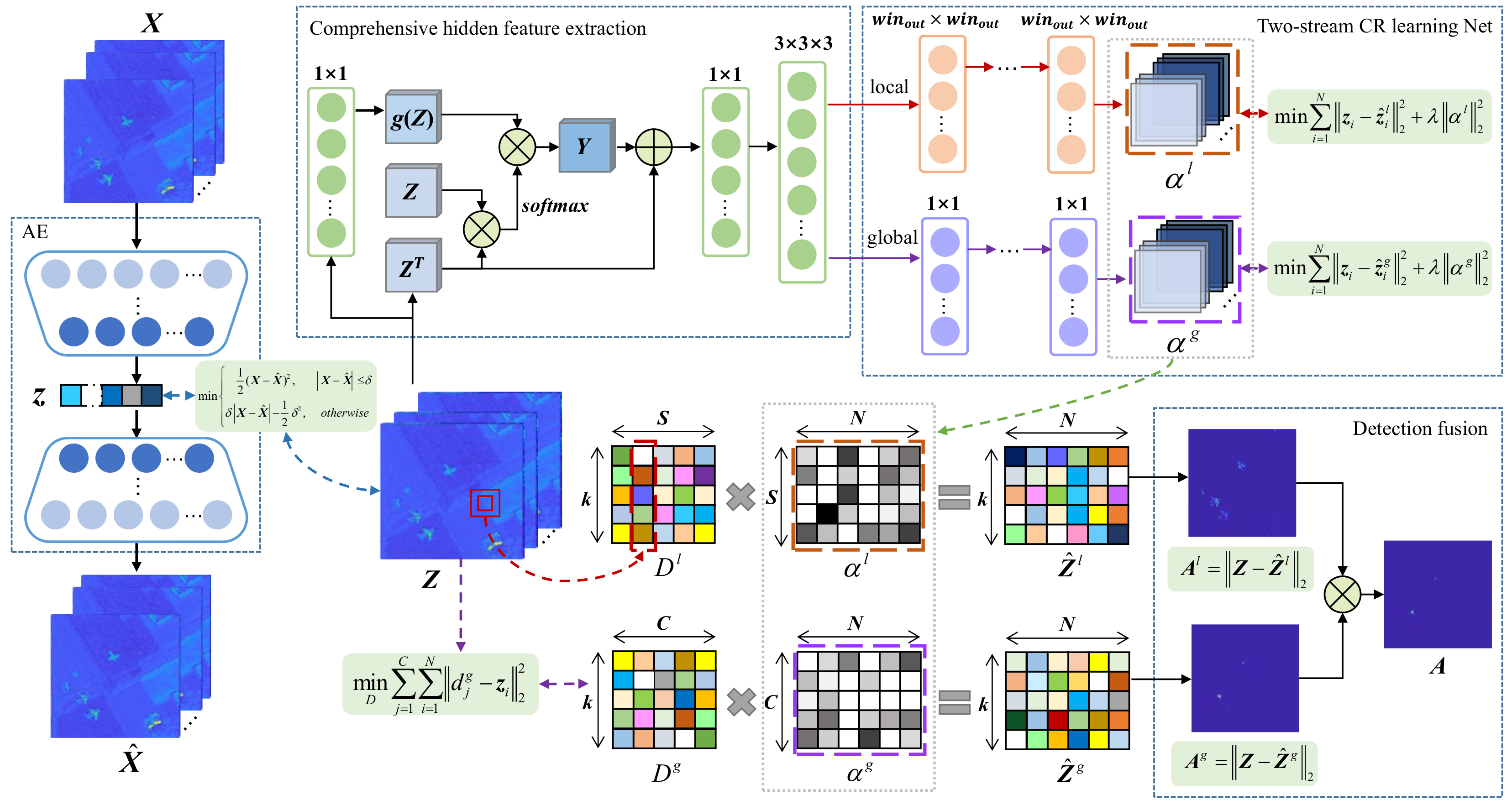
3. Proposed Method
3.1. Hidden Feature Map Generation
3.2. Comprehensive Feature Extraction
3.2.1. Non-Local Module
3.2.2. Local Feature Learning Module
3.3. Two-Stream Collaborative Representation Learning Networks
3.3.1. Global Collaborative Representation Learning
3.3.2. Local Collaborative Representation Learning
3.4. Detection Fusion
| Algorithm 1: Algorithm flow diagram of CRNN |
Input: original Hyperspectral data . Output: Anomaly score map .  |
4. Experiments
4.1. Experimental Settings
4.1.1. Datasets Description
4.1.2. Evaluation Criteria
4.1.3. Compared Method
4.1.4. Implementation Details
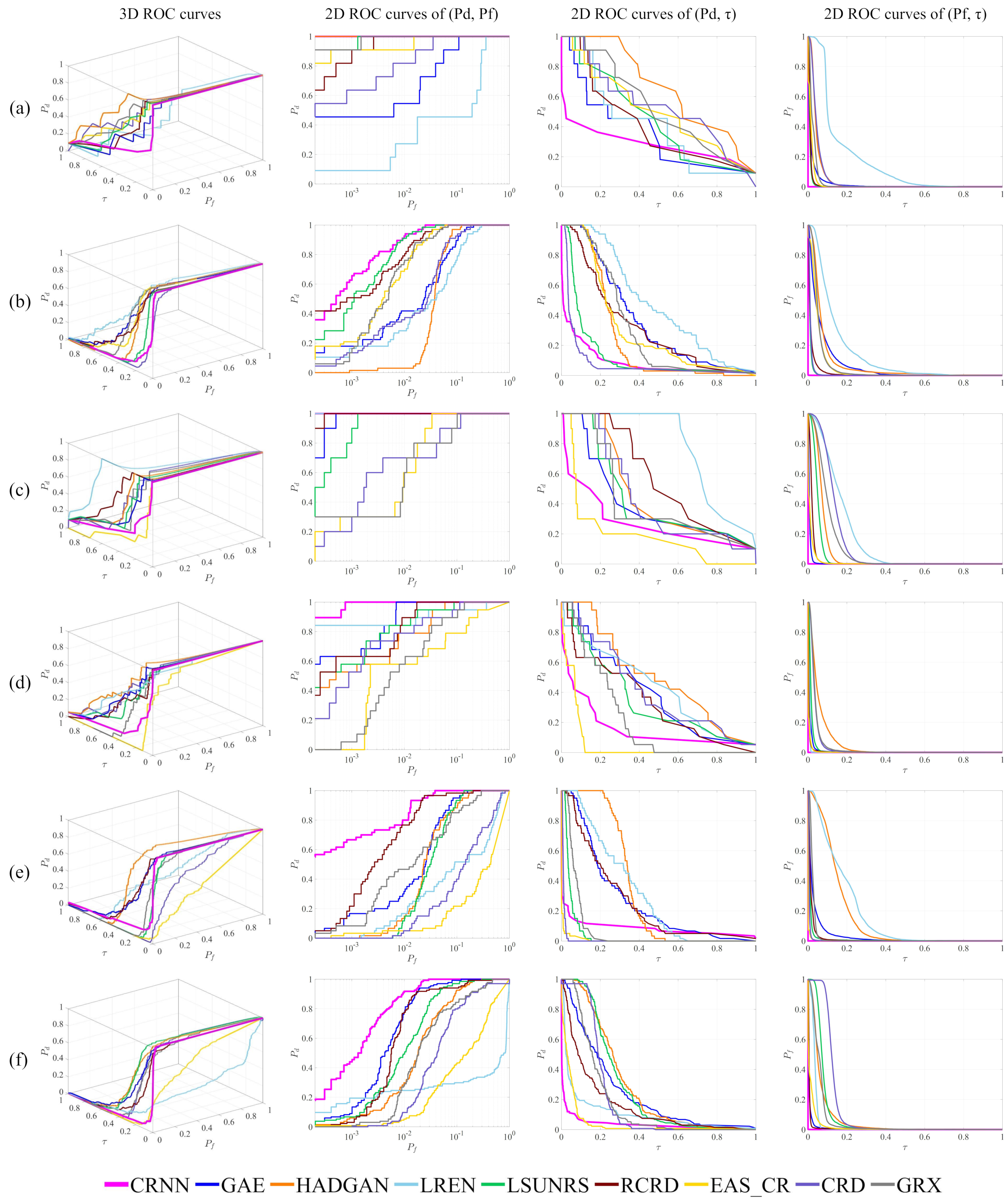
4.2. Detection Performance
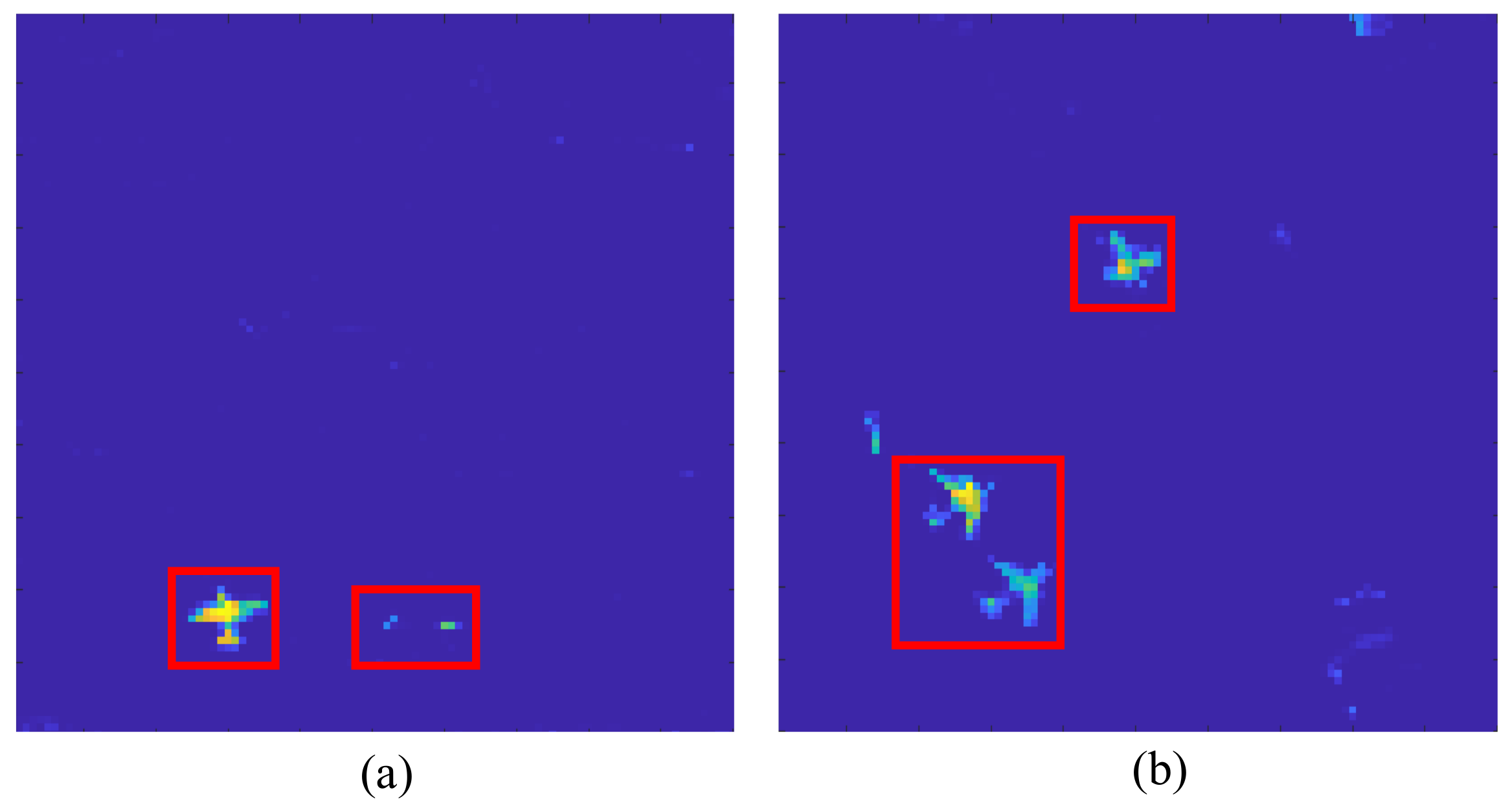
4.2.1. Detection Performance for Small Targets
4.2.2. Detection Performance for Planar Targets
4.2.3. AUC Performance
4.3. Computing Time
5. Discussion
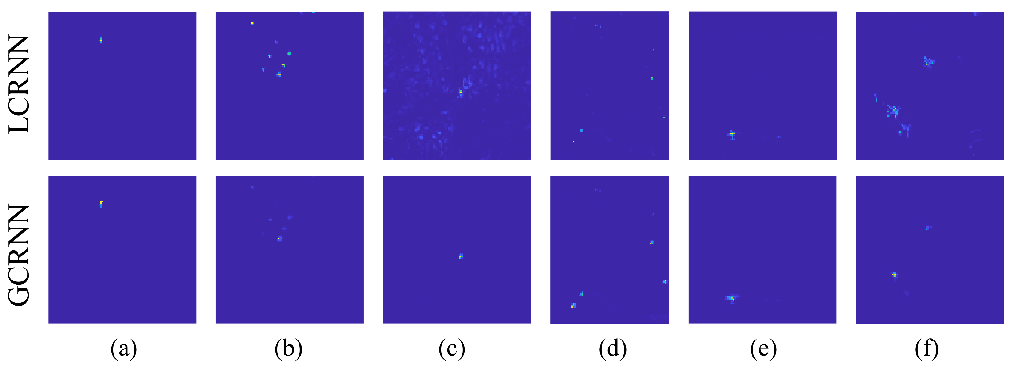
5.1. Ablation Study
- CRNN: the proposed CRNN model, whose detection result is ;
- CRNN+: the CRNN model in additive fusion version, whose detection result is ;
- LCRNN: the local stream of CR networks in CRNN, whose detection result is ;
- GCRNN: the global stream of CR networks in CRNN, whose detection result is ;
- CRNN_se: the local stream and global stream are separately trained and fused to obtain the detection result. It is a separate training version for CRNN;
- LCRNN_se: the local stream of CR networks in CRNN_se;
- GCRNN_se: the global stream of CR networks in CRNN_se.
- (1)
- Global CR and Local CR
- (2)
- Detection Fusion of Global CR and Local CR
- (3)
- Joint Training and Separate Training
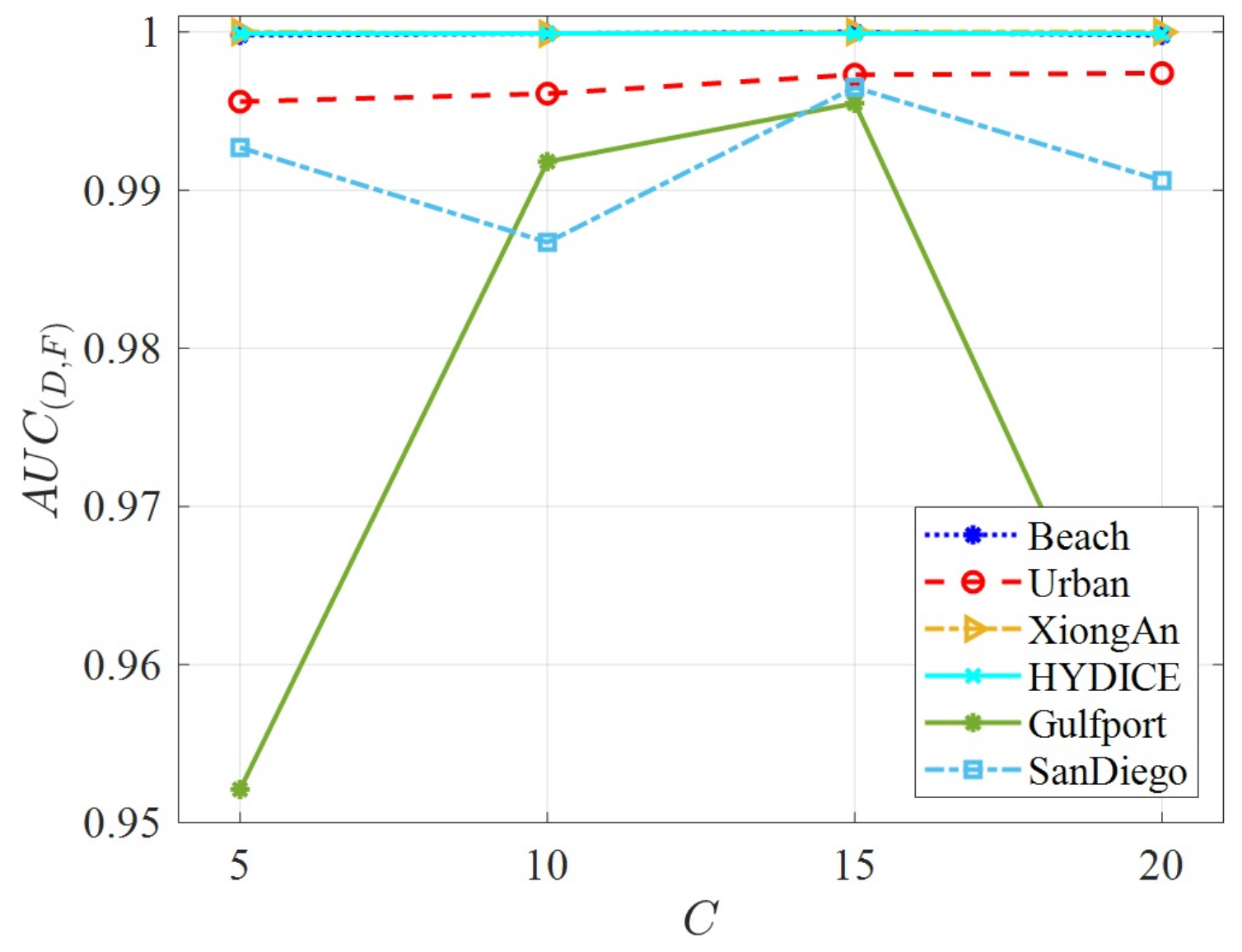
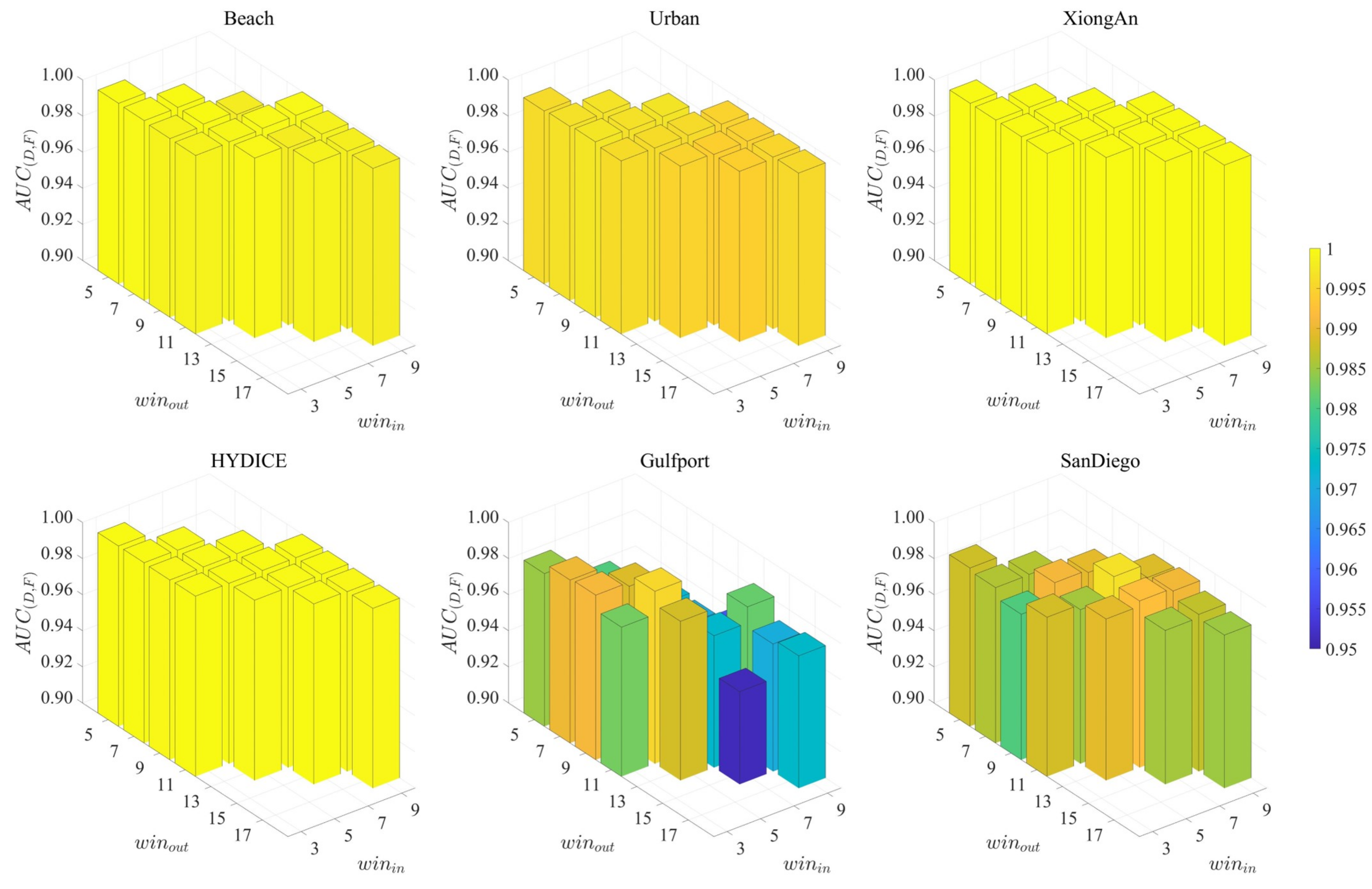
5.2. Parameter Analysis
6. Conclusions
Author Contributions
Funding
Data Availability Statement
Conflicts of Interest
Appendix A

↑ | ↑ | ↓ | ↑ | ↑ | ↑ | ↑ | ↑ | |
|---|---|---|---|---|---|---|---|---|
| CRNN | 1.0000 | 0.2803 | 1.2803 | 2.0000 | 1.2803 | 2.2803 | ||
| CRNN+ | 1.0000 | 0.4354 | 1.4354 | 2.0000 | 1.4354 | 2.4354 | ||
| LCRNN | 0.9999 | 0.2663 | 1.2662 | 1.9999 | 1.2663 | 2.2662 | ||
| GCRNN | 1.0000 | 0.4141 | 1.4141 | 2.0000 | 1.4141 | 2.4141 | ||
| CRNN_se | 1.0000 | 0.1791 | 1.1791 | 2.0000 | 1.1791 | 2.1791 | ||
| LCRNN_se | 0.9984 | 0.2710 | 1.2694 | 1.9978 | 1.2703 | 2.2688 | ||
| GCRNN_se | 1.0000 | 0.2968 | 1.2968 | 2.0000 | 1.2968 | 2.2968 |
↑ | ↑ | ↓ | ↑ | ↑ | ↑ | ↑ | ↑ | |
|---|---|---|---|---|---|---|---|---|
| CRNN | 0.9973 | 0.0899 | 1.0872 | 1.9973 | 1.0899 | 2.0872 | ||
| CRNN+ | 0.9964 | 0.1604 | 1.1567 | 1.9963 | 1.1603 | 2.1566 | ||
| LCRNN | 0.9960 | 0.2255 | 1.2215 | 1.9958 | 1.2254 | 2.2214 | ||
| GCRNN | 0.9961 | 0.0640 | 1.0602 | 1.9961 | 1.0640 | 2.0601 | ||
| CRNN_se | 0.9979 | 0.0504 | 1.0483 | 1.9979 | 1.0504 | 2.0483 | ||
| LCRNN_se | 0.9935 | 0.2495 | 1.2430 | 1.9914 | 1.2474 | 2.2410 | ||
| GCRNN_se | 0.9964 | 0.0828 | 1.0792 | 1.9964 | 1.0827 | 2.0791 |
↑ | ↑ | ↓ | ↑ | ↑ | ↑ | ↑ | ↑ | |
|---|---|---|---|---|---|---|---|---|
| CRNN | 1.0000 | 0.2718 | 1.2718 | 2.0000 | 1.2718 | 2.2718 | ||
| CRNN+ | 1.0000 | 0.5173 | 1.5173 | 1.9943 | 1.5116 | 2.5116 | 90.7 | |
| LCRNN | 0.9999 | 0.4930 | 1.4929 | 1.9919 | 1.4850 | 2.4849 | 61.5 | |
| GCRNN | 0.9998 | 0.2706 | 1.2704 | 1.9997 | 1.2704 | 2.2703 | ||
| CRNN_se | 1.0000 | 0.3773 | 1.3773 | 2.0000 | 1.3773 | 2.3773 | ||
| LCRNN_se | 0.9999 | 0.5628 | 1.5627 | 1.9936 | 1.5565 | 2.5565 | 89.4 | |
| GCRNN_se | 1.0000 | 0.4389 | 1.4389 | 1.9969 | 1.4359 | 2.4359 |
↑ | ↑ | ↓ | ↑ | ↑ | ↑ | ↑ | ↑ | |
|---|---|---|---|---|---|---|---|---|
| CRNN | 0.9999 | 0.1570 | 1.1570 | 1.9999 | 1.1570 | 2.1570 | ||
| CRNN+ | 0.9990 | 0.3518 | 1.3508 | 1.9979 | 1.3508 | 2.3498 | ||
| LCRNN | 0.9998 | 0.3038 | 1.3037 | 1.9994 | 1.3034 | 2.3032 | ||
| GCRNN | 0.9981 | 0.2572 | 1.2553 | 1.9969 | 1.2560 | 2.2541 | ||
| CRNN_se | 0.9997 | 0.1562 | 1.1559 | 1.9997 | 1.1562 | 2.1558 | ||
| LCRNN_se | 0.9948 | 0.3070 | 1.3018 | 1.9918 | 1.3041 | 2.2989 | ||
| GCRNN_se | 0.9990 | 0.2150 | 1.2140 | 1.9988 | 1.2147 | 2.2138 |
↑ | ↑ | ↓ | ↑ | ↑ | ↑ | ↑ | ↑ | |
|---|---|---|---|---|---|---|---|---|
| CRNN | 0.9955 | 0.0843 | 1.0799 | 1.9955 | 1.0843 | 2.0799 | ||
| CRNN+ | 0.9961 | 0.1347 | 1.1308 | 1.9961 | 1.1347 | 2.1308 | ||
| LCRNN | 0.9953 | 0.0934 | 1.0887 | 1.9953 | 1.0933 | 2.0887 | ||
| GCRNN | 0.9904 | 0.0956 | 1.0861 | 1.9904 | 1.0956 | 2.0861 | ||
| CRNN_se | 0.9977 | 0.0445 | 1.0422 | 1.9977 | 1.0445 | 2.0422 | ||
| LCRNN_se | 0.9930 | 0.2548 | 1.2478 | 1.9856 | 1.2475 | 2.2404 | 34.7 | |
| GCRNN_se | 0.9963 | 0.0504 | 1.0468 | 1.9963 | 1.0504 | 2.0467 |
↑ | ↑ | ↓ | ↑ | ↑ | ↑ | ↑ | ↑ | |
|---|---|---|---|---|---|---|---|---|
| CRNN | 0.9965 | 0.0368 | 1.0333 | 1.9965 | 1.0368 | 2.0333 | ||
| CRNN+ | 0.9940 | 0.1284 | 1.1224 | 1.9932 | 1.1275 | 2.1216 | ||
| LCRNN | 0.9926 | 0.1197 | 1.1123 | 1.9916 | 1.1186 | 2.1112 | ||
| GCRNN | 0.9960 | 0.0513 | 1.0473 | 1.9959 | 1.0512 | 2.0472 | ||
| CRNN_se | 0.9915 | 0.0322 | 1.0237 | 1.9913 | 1.0321 | 2.0236 | ||
| LCRNN_se | 0.9855 | 0.0167 | 1.0022 | 1.9832 | 1.0144 | 1.9999 | 7.22 | |
| GCRNN_se | 0.9915 | 0.0634 | 1.0549 | 1.9909 | 1.0629 | 2.0544 |
Appendix B
| Dataset | C | ↑ | ↑ | ↓ | ↑ | ↑ | ↑ | ↑ | ↑ |
|---|---|---|---|---|---|---|---|---|---|
| Beach | 5 | 0.9999 | 0.1939 | 1.1938 | 1.9998 | 1.1939 | 2.1937 | ||
| 10 | 0.9999 | 0.2776 | 1.2775 | 1.9998 | 1.2776 | 2.2775 | |||
| 15 | 1.0000 | 0.2803 | 1.2803 | 2.0000 | 1.2803 | 2.2803 | |||
| 20 | 0.9998 | 0.2025 | 1.2023 | 1.9998 | 1.2025 | 2.2023 | |||
| Urban | 5 | 0.9956 | 0.0668 | 1.0624 | 1.9956 | 1.0668 | 2.0624 | ||
| 10 | 0.9961 | 0.0479 | 1.0439 | 1.9960 | 1.0479 | 2.0439 | |||
| 15 | 0.9973 | 0.0899 | 1.0872 | 1.9973 | 1.0899 | 2.0872 | |||
| 20 | 0.9974 | 0.0879 | 1.0853 | 1.9974 | 1.0879 | 2.0853 | |||
| XiongAn | 5 | 1.0000 | 0.2931 | 1.2931 | 2.0000 | 1.2931 | 2.2931 | ||
| 10 | 0.9999 | 0.3401 | 1.3401 | 1.9999 | 1.3401 | 2.3400 | |||
| 15 | 1.0000 | 0.2718 | 1.2718 | 2.0000 | 1.2718 | 2.2718 | |||
| 20 | 1.0000 | 0.2789 | 1.2789 | 2.0000 | 1.2789 | 2.2788 | |||
| HYDICE | 5 | 0.9999 | 0.1788 | 1.1788 | 2.0000 | 1.1788 | 2.1788 | ||
| 10 | 0.9999 | 0.1873 | 1.1872 | 1.9999 | 1.1873 | 2.1872 | |||
| 15 | 0.9999 | 0.1570 | 1.1570 | 1.9999 | 1.1570 | 2.1570 | |||
| 20 | 0.9999 | 0.2152 | 1.2151 | 1.9999 | 1.2152 | 2.2151 | |||
| Gulfport | 5 | 0.9521 | 0.0098 | 0.9619 | 1.9519 | 1.0095 | 1.9616 | 38.4 | |
| 10 | 0.9919 | 0.0883 | 1.0802 | 1.9918 | 1.0883 | 2.0802 | |||
| 15 | 0.9955 | 0.0843 | 1.0799 | 1.9955 | 1.0843 | 2.0799 | |||
| 20 | 0.9534 | 0.0077 | 0.9611 | 1.9526 | 1.0069 | 1.9604 | 9.79 | ||
| SanDiego | 5 | 0.9928 | 0.0249 | 1.0176 | 1.9923 | 1.0244 | 2.0172 | 52.3 | |
| 10 | 0.9866 | 0.0012 | 0.9878 | 1.9862 | 1.0008 | 1.9874 | 3.12 | ||
| 15 | 0.9965 | 0.0368 | 1.0333 | 1.9965 | 1.0368 | 2.0333 | |||
| 20 | 0.9906 | 0.0143 | 1.0049 | 1.9903 | 1.0140 | 2.0046 | 50.2 |
References
- Eismann, M.T.; Stocker, A.D.; Nasrabadi, N.M. Automated Hyperspectral Cueing for Civilian Search and Rescue. Proc. IEEE 2009, 97, 1031–1055. [Google Scholar] [CrossRef]
- Paoletti, M.; Haut, J.; Plaza, J.; Plaza, A. A new deep convolutional neural network for fast hyperspectral image classification. ISPRS J. Photogramm. Remote Sens. 2018, 145, 120–147. [Google Scholar] [CrossRef]
- Tuia, D.; Flamary, R.; Courty, N. Multiclass feature learning for hyperspectral image classification: Sparse and hierarchical solutions. ISPRS J. Photogramm. Remote Sens. 2015, 105, 272–285. [Google Scholar] [CrossRef] [Green Version]
- Su, H.; Yu, Y.; Du, Q.; Du, P. Ensemble learning for hyperspectral image classification using tangent collaborative representation. IEEE Trans. Geosci. Remote Sens. 2020, 58, 3778–3790. [Google Scholar] [CrossRef]
- Nasrabadi, N.M. Hyperspectral target detection: An overview of current and future challenges. IEEE Signal Process. Mag. 2013, 31, 34–44. [Google Scholar] [CrossRef]
- Axelsson, M.; Friman, O.; Haavardsholm, T.V.; Renhorn, I. Target detection in hyperspectral imagery using forward modeling and in-scene information. ISPRS J. Photogramm. Remote Sens. 2016, 119, 124–134. [Google Scholar] [CrossRef]
- Jiao, C.; Chen, C.; McGarvey, R.G.; Bohlman, S.; Jiao, L.; Zare, A. Multiple instance hybrid estimator for hyperspectral target characterization and sub-pixel target detection. ISPRS J. Photogramm. Remote Sens. 2018, 146, 235–250. [Google Scholar] [CrossRef] [Green Version]
- Chang, C.I. Hyperspectral Anomaly Detection: A Dual Theory of Hyperspectral Target Detection. IEEE Trans. Geosci. Remote Sens. 2022, 60, 1–20. [Google Scholar] [CrossRef]
- Chang, C.I. Target-to-Anomaly Conversion for Hyperspectral Anomaly Detection. IEEE Trans. Geosci. Remote Sens. 2022, 60, 1–28. [Google Scholar] [CrossRef]
- Li, K.; Ling, Q.; Qin, Y.; Wang, Y.; Cai, Y.; Lin, Z.; An, W. Spectral-Spatial Deep Support Vector Data Description for Hyperspectral Anomaly Detection. IEEE Trans. Geosci. Remote Sens. 2022, 60, 1–16. [Google Scholar] [CrossRef]
- Xie, W.; Zhang, X.; Li, Y.; Lei, J.; Li, J.; Du, Q. Weakly Supervised Low-Rank Representation for Hyperspectral Anomaly Detection. IEEE Trans. Cybern. 2021, 51, 3889–3900. [Google Scholar] [CrossRef] [PubMed]
- Su, H.; Wu, Z.; Zhang, H.; Du, Q. Hyperspectral anomaly detection: A survey. IEEE Geosci. Remote Sens. Mag. 2021, 10, 64–90. [Google Scholar] [CrossRef]
- Reed, I.S.; Yu, X. Adaptive multiple-band CFAR detection of an optical pattern with unknown spectral distribution. IEEE Trans. Acoust. Speech Signal Process. 1990, 38, 1760–1770. [Google Scholar] [CrossRef]
- Kwon, H.; Nasrabadi, N.M. Kernel RX-algorithm: A nonlinear anomaly detector for hyperspectral imagery. IEEE Trans. Geosci. Remote Sens. 2005, 43, 388–397. [Google Scholar] [CrossRef]
- Borghys, D.; Kåsen, I.; Achard, V.; Perneel, C. Comparative evaluation of hyperspectral anomaly detectors in different types of background. In Proceedings of the Algorithms and Technologies for Multispectral, Hyperspectral, and Ultraspectral Imagery XVIII, Baltimore, MD, USA, 24 May 2012; Volume 8390, pp. 803–814. [Google Scholar]
- Li, W.; Du, Q. Decision fusion for dual-window-based hyperspectral anomaly detector. J. Appl. Remote Sens. 2015, 9, 097297. [Google Scholar] [CrossRef] [Green Version]
- Guo, Q.; Zhang, B.; Ran, Q.; Gao, L.; Li, J.; Plaza, A. Weighted-RXD and linear filter-based RXD: Improving background statistics estimation for anomaly detection in hyperspectral imagery. IEEE J. Sel. Top. Appl. Earth Obs. Remote Sens. 2014, 7, 2351–2366. [Google Scholar] [CrossRef]
- Chang, C.I. Effective Anomaly Space for Hyperspectral Anomaly Detection. IEEE Trans. Geosci. Remote Sens. 2022, 60, 1–24. [Google Scholar] [CrossRef]
- Carlotto, M.J. A cluster-based approach for detecting human-made objects and changes in imagery. IEEE Trans. Geosci. Remote Sens. 2005, 43, 374–387. [Google Scholar] [CrossRef]
- Hytla, P.C.; Hardie, R.C.; Eismann, M.T.; Meola, J. Anomaly detection in hyperspectral imagery: Comparison of methods using diurnal and seasonal data. J. Appl. Remote Sens. 2009, 3, 033546. [Google Scholar] [CrossRef]
- Banerjee, A.; Burlina, P.; Diehl, C. A support vector method for anomaly detection in hyperspectral imagery. IEEE Trans. Geosci. Remote Sens. 2006, 44, 2282–2291. [Google Scholar] [CrossRef]
- Messinger, D.W.; Albano, J. A graph theoretic approach to anomaly detection in hyperspectral imagery. In Proceedings of the 2011 3rd Workshop on Hyperspectral Image and Signal Processing: Evolution in Remote Sensing (WHISPERS), Lisbon, Portugal, 6–9 June 2011; pp. 1–4. [Google Scholar]
- Yuan, Y.; Ma, D.; Wang, Q. Hyperspectral anomaly detection by graph pixel selection. IEEE Trans. Cybern. 2015, 46, 3123–3134. [Google Scholar] [CrossRef] [PubMed]
- Tao, R.; Zhao, X.; Li, W.; Li, H.C.; Du, Q. Hyperspectral Anomaly Detection by Fractional Fourier Entropy. IEEE J. Sel. Top. Appl. Earth Obs. Remote Sens. 2019, 12, 4920–4929. [Google Scholar] [CrossRef]
- Kang, X.; Zhang, X.; Li, S.; Li, K.; Li, J.; Benediktsson, J.A. Hyperspectral anomaly detection with attribute and edge-preserving filters. IEEE Trans. Geosci. Remote Sens. 2017, 55, 5600–5611. [Google Scholar] [CrossRef]
- Xie, W.; Jiang, T.; Li, Y.; Jia, X.; Lei, J. Structure Tensor and Guided Filtering-Based Algorithm for Hyperspectral Anomaly Detection. IEEE Trans. Geosci. Remote Sens. 2019, 57, 4218–4230. [Google Scholar] [CrossRef]
- Cheng, X.; Wen, M.; Gao, C.; Wang, Y. Hyperspectral Anomaly Detection Based on Wasserstein Distance and Spatial Filtering. Remote Sens. 2022, 14, 2730. [Google Scholar] [CrossRef]
- Shang, W.; Jouni, M.; Wu, Z.; Xu, Y.; Dalla Mura, M.; Wei, Z. Hyperspectral Anomaly Detection Based on Regularized Background Abundance Tensor Decomposition. Remote Sens. 2023, 15, 1679. [Google Scholar] [CrossRef]
- Li, L.; Li, W.; Qu, Y.; Zhao, C.; Tao, R.; Du, Q. Prior-Based Tensor Approximation for Anomaly Detection in Hyperspectral Imagery. IEEE Trans. Neural Networks Learn. Syst. 2022, 33, 1037–1050. [Google Scholar] [CrossRef]
- Chang, C.I.; Lin, C.Y.; Chung, P.C.; Hu, P.F. Iterative Spectral–Spatial Hyperspectral Anomaly Detection. IEEE Trans. Geosci. Remote Sens. 2023, 61, 1–30. [Google Scholar] [CrossRef]
- Li, J.; Zhang, H.; Zhang, L.; Ma, L. Hyperspectral anomaly detection by the use of background joint sparse representation. IEEE J. Sel. Top. Appl. Earth Obs. Remote Sens. 2015, 8, 2523–2533. [Google Scholar] [CrossRef]
- Li, F.; Zhang, X.; Zhang, L.; Jiang, D.; Zhang, Y. Exploiting structured sparsity for hyperspectral anomaly detection. IEEE Trans. Geosci. Remote Sens. 2018, 56, 4050–4064. [Google Scholar] [CrossRef]
- Soofbaf, S.R.; Sahebi, M.R.; Mojaradi, B. A sliding window-based joint sparse representation (swjsr) method for hyperspectral anomaly detection. Remote Sens. 2018, 10, 434. [Google Scholar] [CrossRef] [Green Version]
- Li, W.; Du, Q. Collaborative representation for hyperspectral anomaly detection. IEEE Trans. Geosci. Remote Sens. 2014, 53, 1463–1474. [Google Scholar] [CrossRef]
- Vafadar, M.; Ghassemian, H. Hyperspectral anomaly detection using outlier removal from collaborative representation. In Proceedings of the 2017 3rd International Conference on Pattern Recognition and Image Analysis (IPRIA), Shahrekord, Iran, 19–20 April 2017; pp. 13–19. [Google Scholar]
- Su, H.; Wu, Z.; Du, Q.; Du, P. Hyperspectral anomaly detection using collaborative representation with outlier removal. IEEE J. Sel. Top. Appl. Earth Obs. Remote Sens. 2018, 11, 5029–5038. [Google Scholar] [CrossRef]
- Tu, B.; Li, N.; Liao, Z.; Ou, X.; Zhang, G. Hyperspectral anomaly detection via spatial density background purification. Remote Sens. 2019, 11, 2618. [Google Scholar] [CrossRef] [Green Version]
- Tan, K.; Hou, Z.; Wu, F.; Du, Q.; Chen, Y. Anomaly detection for hyperspectral imagery based on the regularized subspace method and collaborative representation. Remote Sens. 2019, 11, 1318. [Google Scholar] [CrossRef] [Green Version]
- Zhao, C.; Li, C.; Feng, S.; Su, N.; Li, W. A Spectral–Spatial Anomaly Target Detection Method Based on Fractional Fourier Transform and Saliency Weighted Collaborative Representation for Hyperspectral Images. IEEE J. Sel. Top. Appl. Earth Obs. Remote Sens. 2020, 13, 5982–5997. [Google Scholar] [CrossRef]
- Wu, Z.; Su, H.; Tao, X.; Han, L.; Paoletti, M.E.; Haut, J.M.; Plaza, J.; Plaza, A. Hyperspectral Anomaly Detection with Relaxed Collaborative Representation. IEEE Trans. Geosci. Remote Sens. 2022, 60, 1–17. [Google Scholar] [CrossRef]
- Sun, W.; Liu, C.; Li, J.; Lai, Y.M.; Li, W. Low-rank and sparse matrix decomposition-based anomaly detection for hyperspectral imagery. J. Appl. Remote Sens. 2014, 8, 083641. [Google Scholar] [CrossRef]
- Xu, Y.; Wu, Z.; Li, J.; Plaza, A.; Wei, Z. Anomaly detection in hyperspectral images based on low-rank and sparse representation. IEEE Trans. Geosci. Remote Sens. 2015, 54, 1990–2000. [Google Scholar] [CrossRef]
- Zhang, Y.; Du, B.; Zhang, L.; Wang, S. A low-rank and sparse matrix decomposition-based Mahalanobis distance method for hyperspectral anomaly detection. IEEE Trans. Geosci. Remote Sens. 2015, 54, 1376–1389. [Google Scholar] [CrossRef]
- Cheng, T.; Wang, B. Graph and Total Variation Regularized Low-Rank Representation for Hyperspectral Anomaly Detection. IEEE Trans. Geosci. Remote Sens. 2020, 58, 391–406. [Google Scholar] [CrossRef]
- Li, L.; Li, W.; Du, Q.; Tao, R. Low-rank and sparse decomposition with mixture of Gaussian for hyperspectral anomaly detection. IEEE Trans. Cybern. 2020, 51, 4363–4372. [Google Scholar] [CrossRef] [PubMed]
- Abdi, H.; Williams, L.J. Principal component analysis. Wiley Interdiscip. Rev. Comput. Stat. 2010, 2, 433–459. [Google Scholar] [CrossRef]
- Wu, F.; Yang, X.H.; Packard, A.; Becker, G. Induced L2-norm control for LPV systems with bounded parameter variation rates. Int. J. Robust Nonlinear Control 1996, 6, 983–998. [Google Scholar] [CrossRef]
- Zhou, T.; Tao, D. Godec: Randomized low-rank & sparse matrix decomposition in noisy case. In Proceedings of the Proceedings of the 28th International Conference on Machine Learning, ICML 2011, Bellevue, WA, USA, 28 June–2 July 2011. [Google Scholar]
- Jiang, K.; Xie, W.; Lei, J.; Jiang, T.; Li, Y. LREN: Low-rank embedded network for sample-free hyperspectral anomaly detection. In Proceedings of the AAAI Conference on Artificial Intelligence, Vancouver, BC, Canada, 2–9 February 2021; Volume 35, pp. 4139–4146. [Google Scholar]
- Hu, X.; Xie, C.; Fan, Z.; Duan, Q.; Zhang, D.; Jiang, L.; Wei, X.; Hong, D.; Li, G.; Zeng, X.; et al. Hyperspectral anomaly detection using deep learning: A review. Remote Sens. 2022, 14, 1973. [Google Scholar] [CrossRef]
- Lei, J.; Xie, W.; Yang, J.; Li, Y.; Chang, C.I. Spectral–spatial feature extraction for hyperspectral anomaly detection. IEEE Trans. Geosci. Remote Sens. 2019, 57, 8131–8143. [Google Scholar] [CrossRef]
- Lu, X.; Zhang, W.; Huang, J. Exploiting Embedding Manifold of Autoencoders for Hyperspectral Anomaly Detection. IEEE Trans. Geosci. Remote Sens. 2020, 58, 1527–1537. [Google Scholar] [CrossRef]
- Arisoy, S.; Nasrabadi, N.M.; Kayabol, K. GAN-based hyperspectral anomaly detection. In Proceedings of the 2020 28th European Signal Processing Conference (EUSIPCO), Amsterdam, The Netherlands, 18–21 January 2021; pp. 1891–1895. [Google Scholar]
- Jiang, T.; Li, Y.; Xie, W.; Du, Q. Discriminative reconstruction constrained generative adversarial network for hyperspectral anomaly detection. IEEE Trans. Geosci. Remote Sens. 2020, 58, 4666–4679. [Google Scholar] [CrossRef]
- Xie, W.; Liu, B.; Li, Y.; Lei, J.; Chang, C.I.; He, G. Spectral adversarial feature learning for anomaly detection in hyperspectral imagery. IEEE Trans. Geosci. Remote Sens. 2019, 58, 2352–2365. [Google Scholar] [CrossRef]
- Wang, S.; Wang, X.; Zhang, L.; Zhong, Y. Auto-AD: Autonomous Hyperspectral Anomaly Detection Network Based on Fully Convolutional Autoencoder. IEEE Trans. Geosci. Remote Sens. 2022, 60, 1–14. [Google Scholar] [CrossRef]
- Xie, W.; Fan, S.; Qu, J.; Wu, X.; Lu, Y.; Du, Q. Spectral Distribution-Aware Estimation Network for Hyperspectral Anomaly Detection. IEEE Trans. Geosci. Remote Sens. 2022, 60, 1–12. [Google Scholar] [CrossRef]
- Hinton, G.E.; Salakhutdinov, R.R. Reducing the dimensionality of data with neural networks. Science 2006, 313, 504–507. [Google Scholar] [CrossRef] [PubMed] [Green Version]
- Hinton, G.E.; Zemel, R. Autoencoders, minimum description length and Helmholtz free energy. Adv. Neural Inf. Process. Syst. 1994, 6, 3–30. [Google Scholar]
- Goodfellow, I.; Pouget-Abadie, J.; Mirza, M.; Xu, B.; Warde-Farley, D.; Ozair, S.; Courville, A.; Bengio, Y. Generative adversarial nets. Adv. Neural Inf. Process. Syst. 2014, 27, 2672–2680. [Google Scholar]
- Xiang, P.; Ali, S.; Jung, S.K.; Zhou, H. Hyperspectral Anomaly Detection with Guided Autoencoder. IEEE Trans. Geosci. Remote Sens. 2022, 60, 1–18. [Google Scholar] [CrossRef]
- Makhzani, A.; Shlens, J.; Jaitly, N.; Goodfellow, I.; Frey, B. Adversarial autoencoders. arXiv 2015, arXiv:1511.05644. [Google Scholar]
- Xie, W.; Liu, B.; Li, Y.; Lei, J.; Du, Q. Autoencoder and Adversarial-Learning-Based Semisupervised Background Estimation for Hyperspectral Anomaly Detection. IEEE Trans. Geosci. Remote Sens. 2020, 58, 5416–5427. [Google Scholar] [CrossRef]
- Li, Y.; Jiang, T.; Xie, W.; Lei, J.; Du, Q. Sparse Coding-Inspired GAN for Hyperspectral Anomaly Detection in Weakly Supervised Learning. IEEE Trans. Geosci. Remote Sens. 2022, 60, 1–11. [Google Scholar] [CrossRef]
- Huber, P.J. Robust estimation of a location parameter. In Breakthroughs in Statistics; Springer: Berlin, Germany, 1992; pp. 492–518. [Google Scholar]
- Wu, Y.; He, K. Group normalization. In Proceedings of the European Conference on Computer Vision (ECCV), Munich, Germany, 8–14 September 2018; pp. 3–19. [Google Scholar]
- Maas, A.L.; Hannun, A.Y.; Ng, A.Y. Rectifier nonlinearities improve neural network acoustic models. In Proceedings of the ICML, Atlanta, GA, USA, 16–21 June 2013; Volume 30, p. 3. [Google Scholar]
- Wang, X.; Girshick, R.; Gupta, A.; He, K. Non-local neural networks. In Proceedings of the IEEE Conference on Computer Vision and Pattern Recognition, Salt Lake City, UT, USA, 18–23 June 2018; pp. 7794–7803. [Google Scholar]
- Zhang, H.; Goodfellow, I.; Metaxas, D.; Odena, A. Self-attention generative adversarial networks. In Proceedings of the International Conference on Machine Learning, PMLR, Long Beach, CA, USA, 16–18 April 2019; pp. 7354–7363. [Google Scholar]
- Jang, E.; Gu, S.; Poole, B. Categorical reparameterization with gumbel-softmax. arXiv 2016, arXiv:1611.01144. [Google Scholar]
- Senling, C.Y.L.X.Y.W.; Peng, Z. Aerial hyperspectral remote sensing classification dataset of Xiongan New Area (Matiwan Village). J. Remote Sens. 2020, 24, 1299–1306. (In Chinese) [Google Scholar] [CrossRef]
- Zhu, F.; Wang, Y.; Xiang, S.; Fan, B.; Pan, C. Structured sparse method for hyperspectral unmixing. ISPRS J. Photogramm. Remote Sens. 2014, 88, 101–118. [Google Scholar] [CrossRef] [Green Version]
- Chang, C.I. An Effective Evaluation Tool for Hyperspectral Target Detection: 3D Receiver Operating Characteristic Curve Analysis. IEEE Trans. Geosci. Remote Sens. 2021, 59, 5131–5153. [Google Scholar] [CrossRef]
- Chang, C.I. Comprehensive Analysis of Receiver Operating Characteristic (ROC) Curves for Hyperspectral Anomaly Detection. IEEE Trans. Geosci. Remote Sens. 2022, 60, 1–24. [Google Scholar] [CrossRef]
- Belgiu, M.; Drăguţ, L. Random forest in remote sensing: A review of applications and future directions. ISPRS J. Photogramm. Remote Sens. 2016, 114, 24–31. [Google Scholar] [CrossRef]


| Dataset | Sensor | Resolution | Spatial Size | Bands | Anomaly Type | Anomaly Proportion | Anomaly Size |
|---|---|---|---|---|---|---|---|
| Beach | AVIRIS 1 | 4.4 m | 100 × 100 | 188 | boat | 0.61% | 11 |
| Urban | AVIRIS 1 | 17.2 m | 100 × 100 | 204 | buildings | 0.67% | 2–14 |
| HYDICE | HYDICE 2 | 1 m | 80 × 100 | 162 | vehicles | 0.24% | 1–4 |
| XiongAn | Gaofeng 3 | 0.5 m | 100 × 100 | 250 | vehicle | 0.10% | 10 |
| Gulfport | AVIRIS 1 | 3.4 m | 100 × 100 | 188 | 3 airplanes | 0.60% | 10–40 |
| SanDiego | AVIRIS 1 | 3.5 m | 100 × 100 | 188 | 3 airplanes | 0.34% | 30–50 |
| Dataset | Method | ↑ | ↑ | ↓ | ↑ | ↑ | ↑ | ↑ | ↑ |
|---|---|---|---|---|---|---|---|---|---|
| Beach | CRNN | 1.0000 | 0.2803 | 1.2803 | 2.0000 | 1.2803 | 2.2803 | ||
| CRNN_t 1 | 1.0000 | 0.7747 | 0.0014 | 1.7747 | 1.9986 | 1.7733 | 2.7733 | 553.6985 | |
| GAE [61] | 0.9773 | 0.3542 | 0.0176 | 1.3315 | 1.9596 | 1.3366 | 2.3139 | 20.0874 | |
| HADGAN [54] | 1.0000 | 0.6598 | 0.0448 | 1.6597 | 1.9552 | 1.6150 | 2.6150 | 14.7397 | |
| LREN [49] | 0.8451 | 0.4071 | 0.1662 | 1.2521 | 1.6788 | 1.2408 | 2.0859 | 2.4489 | |
| LSUNRS [38] | 0.9998 | 0.4414 | 0.0092 | 1.4413 | 1.9907 | 1.4323 | 2.4321 | 48.1575 | |
| RCRD [40] | 0.9996 | 0.4036 | 0.0114 | 1.4032 | 1.9882 | 1.3922 | 2.3918 | 35.3348 | |
| EAS_CR [18] | 0.9986 | 0.5020 | 0.0149 | 1.5005 | 1.9837 | 1.4871 | 2.4857 | 33.7063 | |
| CRD [34] | 0.9944 | 0.5351 | 0.0469 | 1.5295 | 1.9474 | 1.4882 | 2.4825 | 11.4035 | |
| GRX [13] | 0.9998 | 0.5314 | 0.0259 | 1.5313 | 1.9739 | 1.5055 | 2.5053 | 20.4912 | |
| Urban | CRNN | 0.9973 | 0.0899 | 1.0872 | 1.9973 | 1.0899 | 2.0872 | ||
| CRNN_t 1 | 0.9973 | 0.6896 | 0.0277 | 1.6869 | 1.9696 | 1.6619 | 2.6592 | 24.8633 | |
| GAE [61] | 0.9622 | 0.3695 | 0.0666 | 1.3317 | 1.8956 | 1.3029 | 2.2651 | 5.5496 | |
| HADGAN [54] | 0.9584 | 0.2483 | 0.0763 | 1.2067 | 1.8822 | 1.1720 | 2.1304 | 3.2555 | |
| LREN [49] | 0.9399 | 0.4838 | 0.1406 | 1.4237 | 1.7993 | 1.3432 | 2.2831 | 3.4411 | |
| LSUNRS [38] | 0.9963 | 0.1352 | 0.0105 | 1.1315 | 1.9858 | 1.1247 | 2.1210 | 12.8765 | |
| RCRD [40] | 0.9937 | 0.3162 | 0.0160 | 1.3099 | 1.9777 | 1.3003 | 2.2939 | 19.8251 | |
| EAS_CR [18] | 0.9911 | 0.3082 | 0.0496 | 1.2993 | 1.9414 | 1.2586 | 2.2496 | 6.2098 | |
| CRD [34] | 0.9655 | 0.0848 | 0.0127 | 1.0503 | 1.9528 | 1.0721 | 2.0376 | 6.6565 | |
| GRX [13] | 0.9907 | 0.3143 | 0.0556 | 1.3049 | 1.9351 | 1.2587 | 2.2494 | 5.6570 | |
| XiongAn | CRNN | 1.0000 | 0.2718 | 1.2718 | 2.0000 | 1.2718 | 2.2718 | ||
| CRNN_t 1 | 1.0000 | 0.8708 | 0.2460 | 1.8708 | 1.7540 | 1.6247 | 2.6247 | 3.5392 | |
| GAE [61] | 0.9999 | 0.4014 | 0.0079 | 1.4013 | 1.9920 | 1.3935 | 2.3934 | 50.6621 | |
| HADGAN [54] | 1.0000 | 0.4634 | 0.0718 | 1.4634 | 1.9282 | 1.3917 | 2.3916 | 6.4562 | |
| LREN [49] | 1.0000 | 0.7751 | 0.1641 | 1.7751 | 1.8359 | 1.6109 | 2.6109 | 4.7220 | |
| LSUNRS [38] | 0.9996 | 0.4296 | 0.0499 | 1.4292 | 1.9497 | 1.3797 | 2.3793 | 8.6172 | |
| RCRD [40] | 0.9999 | 0.5710 | 0.0209 | 1.5709 | 1.9791 | 1.5501 | 2.5501 | 27.3467 | |
| EAS_CR [18] | 0.9881 | 0.1909 | 0.0105 | 1.1790 | 1.9776 | 1.1804 | 2.1685 | 18.1455 | |
| CRD [34] | 0.9783 | 0.4413 | 0.1315 | 1.4196 | 1.8469 | 1.3098 | 2.2881 | 3.3569 | |
| GRX [13] | 0.9765 | 0.4222 | 0.1000 | 1.3986 | 1.8765 | 1.3222 | 2.2987 | 4.2235 | |
| HYDICE | CRNN | 0.9999 | 0.1570 | 1.1570 | 1.9999 | 1.1570 | 2.1570 | ||
| CRNN_t 1 | 0.9999 | 0.8132 | 0.0210 | 1.8131 | 1.9790 | 1.7923 | 2.7922 | 38.8089 | |
| GAE [61] | 0.9982 | 0.3973 | 0.0099 | 1.3955 | 1.9883 | 1.3874 | 2.3856 | 40.1662 | |
| HADGAN [54] | 0.9903 | 0.5024 | 0.0571 | 1.4927 | 1.9332 | 1.4453 | 2.4356 | 8.7944 | |
| LREN [49] | 0.9784 | 0.4271 | 0.0093 | 1.4055 | 1.9691 | 1.4179 | 2.3963 | 46.1746 | |
| LSUNRS [38] | 0.9929 | 0.3449 | 0.0166 | 1.3378 | 1.9763 | 1.3283 | 2.3212 | 20.7202 | |
| RCRD [40] | 0.9962 | 0.3380 | 0.0059 | 1.3342 | 1.9903 | 1.3322 | 2.3284 | 57.7771 | |
| EAS_CR [18] | 0.9233 | 0.0554 | 0.0037 | 0.9787 | 1.9196 | 1.0517 | 1.9751 | 15.0686 | |
| CRD [34] | 0.9868 | 0.4117 | 0.0351 | 1.3985 | 1.9517 | 1.3765 | 2.3634 | 11.7149 | |
| GRX [13] | 0.9763 | 0.2184 | 0.0380 | 1.1947 | 1.9382 | 1.1803 | 2.1566 | 5.7406 | |
| Gulfport | CRNN | 0.9955 | 0.0843 | 1.0799 | 1.9955 | 1.0843 | 2.0799 | ||
| CRNN_t 1 | 0.9955 | 0.4825 | 0.0105 | 1.4780 | 1.9851 | 1.4720 | 2.4676 | 46.1582 | |
| GAE [61] | 0.9690 | 0.2675 | 0.0314 | 1.2364 | 1.9376 | 1.2361 | 2.2051 | 8.5239 | |
| HADGAN [54] | 0.9602 | 0.3380 | 0.1496 | 1.2982 | 1.8106 | 1.1884 | 2.1486 | 2.2588 | |
| LREN [49] | 0.7521 | 0.3104 | 0.1739 | 1.0626 | 1.5782 | 1.1365 | 1.8887 | 1.7851 | |
| LSUNRS [38] | 0.9589 | 0.0455 | 0.0139 | 1.0044 | 1.9450 | 1.0316 | 1.9905 | 3.2769 | |
| RCRD [40] | 0.9899 | 0.2552 | 0.0160 | 1.2451 | 1.9739 | 1.2392 | 2.2291 | 15.9448 | |
| EAS_CR [18] | 0.5714 | 0.0059 | 0.0015 | 0.5773 | 1.5698 | 1.0044 | 1.5758 | 3.8782 | |
| CRD [34] | 0.7762 | 0.0112 | 0.0069 | 0.7874 | 1.7693 | 1.0043 | 1.7805 | 1.6246 | |
| GRX [13] | 0.9526 | 0.0736 | 0.0248 | 1.0262 | 1.9278 | 1.0489 | 2.0015 | 2.9743 | |
| SanDiego | CRNN | 0.9965 | 0.0368 | 1.0333 | 1.9965 | 1.0368 | 2.0333 | ||
| CRNN_t 1 | 0.9965 | 0.5481 | 0.0178 | 1.5446 | 1.9787 | 1.5303 | 2.5268 | 30.7612 | |
| GAE [61] | 0.9910 | 0.2380 | 0.0079 | 1.2290 | 1.9831 | 1.2301 | 2.2211 | 30.1127 | |
| HADGAN [54] | 0.9644 | 0.2898 | 0.0653 | 1.2542 | 1.8991 | 1.2244 | 2.1888 | 4.4353 | |
| LREN [49] | 0.4387 | 0.1041 | 0.0346 | 0.5428 | 1.4041 | 1.0695 | 1.5082 | 3.0098 | |
| LSUNRS [38] | 0.9796 | 0.2756 | 0.0789 | 1.2552 | 1.9007 | 1.1967 | 2.1763 | 3.4914 | |
| RCRD [40] | 0.9825 | 0.1575 | 0.0084 | 1.1399 | 1.9740 | 1.1490 | 2.1315 | 18.6983 | |
| EAS_CR [18] | 0.7515 | 0.0464 | 0.0149 | 0.7979 | 1.7366 | 1.0316 | 1.7831 | 3.1202 | |
| CRD [34] | 0.9071 | 0.1993 | 0.1272 | 1.1064 | 1.7799 | 1.0721 | 1.9792 | 1.5671 | |
| GRX [13] | 0.9403 | 0.1778 | 0.0589 | 1.1181 | 1.8814 | 1.1189 | 2.0592 | 3.0176 |
↑ | ↑ | ↓ | ↑ | ↑ | ↑ | ↑ | ↑ | |
|---|---|---|---|---|---|---|---|---|
| CRNN | 0.9982 | 0.1534 | 1.1516 | 1.9982 | 1.1534 | 2.1516 | ||
| CRNN_t 1 | 0.9982 | 0.6965 | 0.0541 | 1.6947 | 1.9441 | 1.6424 | 2.6406 | 116.3049 |
| GAE [61] | 0.9829 | 0.3380 | 0.0236 | 1.3209 | 1.9594 | 1.3144 | 2.2974 | 25.8503 |
| HADGAN [54] | 0.9789 | 0.4169 | 0.0775 | 1.3958 | 1.9014 | 1.3395 | 2.3183 | 6.6567 |
| LREN [49] | 0.8257 | 0.4179 | 0.1148 | 1.2436 | 1.7109 | 1.3032 | 2.1289 | 10.2636 |
| LSUNRS [38] | 0.9879 | 0.2787 | 0.0298 | 1.2666 | 1.9580 | 1.2489 | 2.2367 | 16.1900 |
| RCRD [40] | 0.9936 | 0.3403 | 0.0131 | 1.3339 | 1.9805 | 1.3272 | 2.3208 | 29.1545 |
| EAS_CR [18] | 0.8706 | 0.1848 | 0.0159 | 1.0555 | 1.8548 | 1.1690 | 2.0396 | 13.3548 |
| CRD [34] | 0.9347 | 0.2806 | 0.0601 | 1.2153 | 1.8747 | 1.2205 | 2.1552 | 6.0539 |
| GRX [13] | 0.9727 | 0.2896 | 0.0505 | 1.2623 | 1.9222 | 1.2391 | 2.2118 | 7.0174 |
| Mean | Variance(%) | Mean | Variance(%) | Mean | Variance(%) | |
|---|---|---|---|---|---|---|
| Beach | 0.99950 | 0.04849 | 0.22151 | 4.75515 | 0.00432 | |
| Urban | 0.99642 | 0.10841 | 0.07129 | 1.24275 | 0.00110 | |
| XiongAn | 0.99994 | 0.00611 | 0.2561 | 4.02692 | 0.00242 | |
| HYDICE | 0.99988 | 0.00953 | 0.18799 | 3.54861 | 0.00070 | |
| Gulfport | 0.98564 | 1.36994 | 0.08248 | 2.59059 | 0.02073 | |
| SanDiego | 0.98954 | 0.43000 | 0.02573 | 1.11803 | 0.01517 | |
| CRNN | GAE [61] | HADGAN [54] | LREN [49] | LSUNRS [38] | RCRD [40] | EAS_CR [18] | CRD [34] | GRX [13] | |
|---|---|---|---|---|---|---|---|---|---|
| Beach | 49.8535 (0.0279) | 47.7064 (6.4304) | 674.0821 (1.8471) | 100.2248 | 18.7829 | 38.2593 | 2.5918 | 1.5395 | 0.0854 |
| Urban | 60.6503 (0.0259) | 48.6605 (6.4776) | 677.5559 (2.0005) | 109.0844 | 19.3547 | 40.2936 | 3.1943 | 1.6119 | 0.0896 |
| XiongAn | 21.0506 (0.0558) | 56.7479 (7.9990) | 673.0219 (2.6153) | 102.5597 | 30.9906 | 51.7006 | 3.3039 | 8.8312 | 0.1826 |
| HYDICE | 19.2016 (0.0189) | 26.0721 (5.2584) | 693.5843 (1.6805) | 73.0596 | 14.5599 | 25.5156 | 1.6684 | 1.2025 | 0.0669 |
| Gulfport | 70.5033 (0.0488) | 47.8685 (6.4286) | 676.432 (1.8710) | 100.8034 | 18.8575 | 39.4005 | 2.6521 | 1.5377 | 0.0807 |
| SanDiego | 31.5995 (0.0229) | 48.6626 (6.7521) | 676.4849 (1.8861) | 101.3657 | 19.0317 | 36.6709 | 2.1232 | 1.5573 | 0.0840 |
↑ | ↑ | ↓ | ↑ | ↑ | ↑ | ↑ | ↑ | |
|---|---|---|---|---|---|---|---|---|
| CRNN | 0.9982 | 0.1534 | 1.1516 | 1.9982 | 1.1534 | 2.1516 | ||
| CRNN+ | 0.9976 | 0.2880 | 1.2856 | 1.9963 | 1.2867 | 2.2843 | ||
| LCRNN | 0.9973 | 0.2503 | 1.2475 | 1.9956 | 1.2487 | 2.2459 | ||
| GCRNN | 0.9968 | 0.1921 | 1.1889 | 1.9965 | 1.1919 | 2.1887 | ||
| CRNN_se | 0.9978 | 0.1400 | 1.1377 | 1.9977 | 1.1399 | 2.1377 | ||
| LCRNN_se | 0.9942 | 0.2770 | 1.2712 | 1.9906 | 1.2734 | 2.2676 | ||
| GCRNN_se | 0.9972 | 0.1912 | 1.1884 | 1.9966 | 1.1906 | 2.1878 |
Disclaimer/Publisher’s Note: The statements, opinions and data contained in all publications are solely those of the individual author(s) and contributor(s) and not of MDPI and/or the editor(s). MDPI and/or the editor(s) disclaim responsibility for any injury to people or property resulting from any ideas, methods, instructions or products referred to in the content. |
© 2023 by the authors. Licensee MDPI, Basel, Switzerland. This article is an open access article distributed under the terms and conditions of the Creative Commons Attribution (CC BY) license (https://creativecommons.org/licenses/by/4.0/).
Share and Cite
Duan, Y.; Ouyang, T.; Wang, J. CRNN: Collaborative Representation Neural Networks for Hyperspectral Anomaly Detection. Remote Sens. 2023, 15, 3357. https://doi.org/10.3390/rs15133357
Duan Y, Ouyang T, Wang J. CRNN: Collaborative Representation Neural Networks for Hyperspectral Anomaly Detection. Remote Sensing. 2023; 15(13):3357. https://doi.org/10.3390/rs15133357
Chicago/Turabian StyleDuan, Yuxiao, Tongbin Ouyang, and Jinshen Wang. 2023. "CRNN: Collaborative Representation Neural Networks for Hyperspectral Anomaly Detection" Remote Sensing 15, no. 13: 3357. https://doi.org/10.3390/rs15133357