Identifying the Optimal Radiometric Calibration Method for UAV-Based Multispectral Imaging

Abstract

The development of UAVs and multispectral cameras has led to remote sensing applications with unprecedented spatial resolution. However, uncertainty remains on the radiometric calibration process for converting raw images to surface reflectance. Several calibration methods exist, but the advantages and disadvantages of each are not well understood. We performed an empirical analysis of five different methods for calibrating a 10-band multispectral camera, the MicaSense RedEdge MX Dual Camera System, by comparing multispectral images with spectrometer measurements taken in the field on the same day. Two datasets were collected, one in clear-sky and one in overcast conditions on the same field. We found that the empirical line method (ELM), using multiple radiometric reference targets imaged at mission altitude performed best in terms of bias and RMSE. However, two user-friendly commercial solutions relying on one single grey reference panel were only slightly less accurate and resulted in sufficiently accurate reflectance maps for most applications, particularly in clear-sky conditions. In overcast conditions, the increase in accuracy of more elaborate methods was higher. Incorporating measurements of an integrated downwelling light sensor (DLS2) did not improve the bias nor RMSE, even in overcast conditions. Ultimately, the choice of the calibration method depends on required accuracy, time constraints and flight conditions. When the more accurate ELM is not possible, commercial, user-friendly solutions like the ones offered by Agisoft Metashape and Pix4D can be good enough.

1. Introduction

The development of unmanned aerial vehicle (UAV) and spectral cameras has caused a breakthrough in the field of remote sensing (RS) by enabling the collection of imagery at specific wavelengths with unprecedented spatial resolution [1,2]. Remotely sensed multispectral images have been used in precision agriculture to assess nitrogen [3] and chlorophyll content [4], growth, yield, health status, and disease [1,5]. To this end, several manufacturers have developed multispectral cameras specifically for UAV applications. Most cameras have been designed with a separate sensor for each band (examples are the MicaSense RedEdge, Tetracam MCA or DJI Multispectral camera systems). These solutions have been developed with user friendliness in mind; they come or are compatible with integrated global navigation satellite system (GNSS) systems, irradiance sensors and have built-in compatibility with most common image processing software packages. The possible drawback is that high user-friendliness requirements have led to simplifications in the workflow. These simplifications have their effect on the recommended workflow for capturing data, as well as on the image processing stage, possibly affecting radiometric calibration [6]. This reduction in accuracy has not yet been quantified, though.

Multispectral images need to be converted into reflectance data before they can be interpreted or used as input for calculating vegetation indices (VI). This process, called radiometric calibration, has been repeatedly identified as one of the main technological barriers to using UAVs for remote sensing [7]. Many different approaches for radiometric calibration have been proposed, but only some are implemented in commercial software packages or are easily available through open source software [8,9,10,11]. Using commercial software has drawbacks: software developers usually limit the users’ insight in the specifics of the processing pipeline [12]. Furthermore, actively developed packages are continually updated, and each update can change (part of) the calibration workflow. This complicates the comparison of datasets processed with different versions or packages. However, using commercial software is by far the fastest and easiest method to convert raw images into a usable reflectance map. Open source packages are usually developed with a reduced emphasis on user friendliness and therefore require a higher level of expertise, increasing the barrier of entry for potential users. Additionally, open source packages are usually less frequently updated and are more likely to contain bugs or errors in their workflow. Unlike commercial software, they do provide complete insight into the process. One example of an open source radiometric calibration solution is the Python package developed by MicaSense at https://github.com/micasense/imageprocessing (accessed on 24 February 2023) [10]. In scientific literature, several methods for radiometric calibration have been described that are not easily available as well (e.g., [13,14]). These methods require a custom implementation to use, and might depend on specific sensors that are not always available to other users. Intuitively, more complex methods require less assumptions than more simplified methods and should therefore lead to more accurate calibrations. However, the extent of the improvement with more complex algorithms remains unclear.

The performance of radiometric calibration methods also depends on the circumstances at the moment of data collection. Some methods might be highly suited to deal with varying illumination conditions, but less suited for clear-sky conditions or vice versa. For example, the MicaSense Dual Camera system comes with a DLS2 irradiance sensor, which is capable of measuring solar irradiance as well as the solar incidence angle. However, the use of corrections based on this sensor in clear-sky conditions is discouraged by the manufacturer. The impact of meteorological conditions on method performances is something that few studies take into account when comparing methods. In this article, we test and compare five different radiometric calibration methods, ranging from very user-friendly but possibly simplistic to more complex methods, requiring additional measurements in the field and additional pre-processing power. These methods are evaluated with probably the most wide-spread multispectral camera (MicaSense RedEdge), and are tested on a sunny and an overcast dataset. Before providing the full description of the methods (Section 3) and the results (Section 4), we first give a more detailed background on radiometric calibration (Section 2).

2. Background on Radiometric Calibration

Images are subject to two main types of radiometric deviations: sensor effects and environmental effects. Sensor effects are present because each sensing system has its specific physical characteristics that affect the translation of incoming photons into an electrical signal; environmental effects are caused by meteorological conditions influencing the surface radiant flux [15,16,17]. The aim of radiometric calibration is to remove these effects as much as possible [11,17,18].

2.1. Sensor Corrections

Sensor- and environmental corrections each require different methodologies. Usually, sensor effects are first corrected for in the processing pipeline. Initially, raw images (in digital number (DN)) are converted to normalized DN images (DN_n). When reflectance maps are the intended end product, results are improved by performing absolute radiometric sensor correction. This involves converting unitless DN_n into at-sensor radiance L$\left(\frac{W}{m^2\times Sr\times nm}\right)$, according to the formula

$$L(x,y)=V_{(x,y)}\times \frac{a_1}{g}\times \frac{p(x,y)-p_{BL}(x,y)}{t_e+a_{2}y-a_3{t}_{e}y}$$

(1)

where the radiance $L(x,y)$ for each pixel with coordinates $(x,y)$ is represented in terms of $V_{(x,y)}$, the vignetting correction; g, the sensor gain; $p(x,y)$ and $p_{BL}(x,y)$, the normalized raw DN and normalized black level DN; $t_e$, the exposure time; and $a_1, a_2$ and $a_3$ representing the radiometric correction factors [10,15,19]. The sensor-specific constants $a_{1-3}$ need to be determined empirically in lab conditions and are usually provided by sensor manufacturers. However, in the case where researchers performed their own additional sensor calibration and re-assessed $a_{1-3}$, the accuracy of the reflectance images increased [15]. Additionally, these constants are not likely to be constant during the entire lifetime of a sensor. This emphasizes the need for thorough, transparent and reliable calibration workflows, and timely recalibrations.

2.2. Environmental Corrections

After correcting for sensor effects and determining the at-sensor irradiance, images need correction for factors that cause deviations between the at-sensor radiance and the surface reflectance: (i) meteorological conditions, including the ratio between direct and diffuse illumination; (ii) the sun-object-sensor angle; and (iii) the atmospheric absorption and scattering between the object and the sensor [11]. Correction for these effects requires in situ reference measurements, for which two approaches are commonly used (or combined): absolute radiometric calibration and the empirical line method (ELM) [11,16,18,20,21].

2.2.1. Absolute Radiometric Correction

Absolute radiometric correction, sometimes called vicarious correction, involves using irradiance sensors to continually measure the incoming solar irradiance during a mission. The irradiance measurements can be used to convert calibrated images to reflectance by dividing radiance (captured by the camera) by irradiance (captured by the sensor) after calibration of both sensors [18,20,22]. The irradiance sensor needs to capture the irradiance in the same spectral bands as the camera, which can be achieved by using identical physical filters, or through resampling hyperspectral measurements to match the multispectral camera’s bands and their respective bandwidths [23]. Since all sensors and filters have their specific spectral response curves, hyperspectral measurements for calibration should be scaled accordingly. Unfortunately, the response curves for sensing systems are rarely disclosed by manufacturers, and determining them requires specialized equipment [15,24]. Still, even with sub-optimal reference measurements, accurate reflectance maps have been generated using the absolute radiometric correction method [22].

Two major approaches for absolute radiometric correction have been proposed: either placing the irradiance sensor at ground level or mounting it on top of the UAV. An irradiance sensor prevents the UAV tilt and angle from affecting the measurements. However, changes in irradiance are not uniformly distributed over the surface, meaning that the UAV can be flying over an area shadowed by clouds while the irradiance sensor stands in a sunny spot. Mounting the irradiance sensor on top of the UAV largely solves this problem, but brings the challenge of tilt and roll of the UAV affecting the irradiance measurements. This can be solved through mounting the sensor on an upward-facing gimbal, but this is technically challenging and to our knowledge not yet operational [25]. Alternatively, irradiance measurements can be corrected for UAV orientation during data processing based on inertial measurement unit (IMU) or photogrammetry data [26]. For accurate corrections, the irradiance sensor should always be oriented at a reciprocal angle to the camera, regardless of UAV orientation [18].

Absolute radiometric correction assumes that the atmosphere between the ground and the camera does not influence the signal, which is reasonable for typical flying altitudes of 100 m or less, though site- and weather dependent as the presence of aerosols, airborne dust or other pollutants can affect the measured signal. The main way to be certain that this effect does not influence the data quality is to use reference targets at ground level.

2.2.2. The Empirical Line Method

The ELM consists of finding the linear relationship between the at-sensor irradiance and the surface reflectance at ground level, usually through the use of radiometric reference targets (RRT) in the form of panels with uniform spectra [16,27,28], while the key idea behind the ELM is straightforward, many different approaches have been published. Some of the factors that vary between different implementations are (i) the number of panels used, (ii) the handling of pixels that fall outside of the expected reflectance range, (iii) whether the reflectance of reference panels is determined in situ or in lab conditions, and (iv) distance at which the imaging sensor measures the RRT(s).

(i)

The number of RRTs that are used varies a lot between publications, ranging from just one, to 8 or more panels [29,30,31,32,33]. Theoretically, two panels are needed to determine an accurate slope and intercept for the linear relationship between at-sensor radiance and surface reflectance [21]. When the intercept is assumed constant, an even easier method can be used: the simplified ELM [29]. This method requires just one RRT. Due to its simplicity, the simplified ELM was adopted by several manufacturers, including MicaSense. However, a recent study has indicated that reflectance values outside of the reflectance range of reference targets are less accurately calibrated [33]. While it is theoretically true that only two RRTs are necessary for accurately calibrating a single band, the gray level of these panels matters. The reflectance range should not be too narrow nor should measurements of a panel be saturated in a given band [29,33,34,35]. For multispectral cameras, the number of used RRTs should therefore depend on the bands of the camera, making sure that the RRTs cover most of the expected intensity range for each band. This indicates that the simplified ELM might reduce the accuracy of reflectance images, as the expected intensity ranges in the RGB spectrum and near infra-red (NIR) spectrum are very different.

(ii)

Slight inaccuracies during capture and calibration of remotely sensed images can lead to a small percentage of pixels reaching reflectance values below 0. Physically, a reflection value below 0 is not possible, as no material can absorb or transmit more photons than the ones that reach it. Furthermore, these pixels can cause errors. For example, when the reflectance data is used for calculating visual indices (VI)s, clipping negative values to 0 can cause divisions to result in NaN values. As a solution, Tu et al. (2018) proposed shifting calibrated reflectance images, so that the new minimum becomes 0 [34]. Others have attributed the negative values to shadows and treated them as outliers [19].

(iii)

The reflectance of reference targets can be determined in lab conditions or in the field. Both methods have advantages and disadvantages. Depending on the material the reference targets are made of, their behavior will be more or less similar to a perfect Lambertian surface. As many authors work with self-painted Masonite or wooden panels, their bidirectional reflectance distribution function will not be perfectly Lambertian surfaces [11,29]. Consequently, the angle at which these panels are measured, combined with the solar incidence angle, will have an impact on the reference measurements. When measuring the reference targets in the field, requirements for the Lambertian behavior of reference targets is lower, as the solar incidence angle can be assumed constant for relatively short RS missions, or with frequent measurement of the reference target(s). When the reflectance of reference targets is determined in lab conditions, the requirements for reference targets is higher, as the solar incidence angle must not influence the measured reflectance. With such high-end reflectance targets, in situ spectrometer measurements are not needed, reducing the workload of a mission. However, reference targets that are used regularly are subjected to the elements. Wear, radiation and dirt can affect the reflectance, requiring frequent maintenance and recalibration of reference targets if they were determined in lab conditions.

(iv)

Different methods for capturing the reference image(s) on which the radiometric calibration is based have been proposed. The recommended method for MicaSense cameras requires the user to capture a reference image by carrying the UAV over a reference target that was calibrated by MicaSense. In doing so, part of the hemisphere will be blocked from the reference panel by the UAV and the user carrying the device, even when no direct shadow is cast onto the panel, meaning that the diffuse solar irradiance will not be accurately measured, possibly introducing errors in further calibration steps [6]. Furthermore, measuring reflectance at ground level entails that any scattering or absorption of light on the path from the surface to the sensor will not be corrected for. Instead, capturing reference images from the same altitude as the mission altitude seems a better option. This does however require sufficiently large reference targets (5 times the ground sampling distance (GSD) is a good rule of thumb) so enough pure pixels represent the reference targets, and do not contain mixed information from the surface below the panels [18]. Near-Lambertian panels (e.g., from Spectralon) of that size are expensive, impractical to produce and even more prone to damage than smaller counterparts, so measuring reference targets at altitude usually requires concessions in reference target quality, increasing the need for in situ surface reflectance determination.

Especially in overcast conditions, the ELM alone does not suffice for generating accurate reflectance maps [18]. A common solution for this is to use an irradiance sensor to correct for variations in incoming radiation, essentially combining the absolute radiometric corrections and ELM workflows. Applying the ELM after correction for irradiance can then result in more accurate reflectance maps than either the ELM or the absolute radiometric correction method alone [30]. An example of this workflow is the intended workflow for MicaSense multispectral cameras with their DLS2 irradiance sensor.

Few publications directly compare different existing methods, and findings of those studies do not always match. For example, Jiang et al., (2022) found that corrections done through Metashape were more accurate than their implementation of the ELM on an orthomosaic [19]. On the other hand, Svensgaard et al., (2021) found that their implementation of the ELM outperformed corrections done through the Pix4D software package [36]. The difference in correction methods between the two commonly used commercial software packages Metashape and Pix4D is not clear, as both have implemented their methods based on the same hardware, namely the use of a single RRT, and, optionally, an irradiance sensor, while both packages are capable of generating reflectance maps of reasonable quality [22], it is unclear if the implemented methods have room for improvement, or if the added value of newer, more sophisticated methods is significant. Moreover, it is unclear what the performance is of the incoming light sensors integrated with most multispectral sensors. Qin et al., (2022) found that the recommended workflow by MicaSense outperformed 4 other calibration methods in varying illumination conditions [37]. Comparing the radiometric calibration methods used by the aforementioned studies based on their results alone is not possible, as flight circumstances undoubtedly influence the performance of calibration methods. Anticipating the need for transparent, well characterized radiometric calibration protocols, we performed a case study to assess the performance of several commonly used calibration approaches, and one variation on the ELM, on identical datasets in different illumination conditions.

3. Material and Methods

3.1. Field Work

Aerial imagery was captured using a DJI Matrice 600 Pro UAV on 3 October 2022 and 6 October 2022, in overcast and clear-sky conditions, respectively. An overview of the relevant flight conditions is given in

Table 1. Overview of the circumstances for each flight. Cloud cover data were obtained from a nearby weather station [38].

	Overcast Flight	Clear-Sky Flight
Date	3 October 2022	6 October 2022
Start time	11 h 49	11 h 22
End time	12 h 10	11 h 37
Cloud cover (%)	100	0
Ground sampling distance (m)	0.03	0.02

. The site was an experimental field located in Bottelare, Belgium (Figure 1). Cloud coverage data were obtained from the nearest weather station, 4.2 km from the site [38], while this weather station reports a 100% overcast sky on 3 October, illumination varied during the flight. The UAV was equipped with a MicaSense RedEdge Dual MX Camera system, which has a down-welling light sensor (DLS2) (AgEagle, Wichita, KS, USA). The camera records 10 spectral bands (

Table 2. Multispectral camera band properties of both cameras in the dual camera system.

Camera Number	Band Number	Band Name	Center Wavelength (nm)	Band Width (nm)
1	2	Blue	475	32
1	4	Green	560	27
1	6	Red	668	14
1	8	Red Edge	717	12
1	10	Near Infrared	842	57
2	1	Coastal Blue	444	28
2	3	Green	531	14
2	5	Red	650	16
2	7	Red Edge	705	10
2	9	Red Edge	740	18

) and was mounted on a T3V3 gimbal (Gremsy, Ho Chi Minh City, Vietnam). The camera was pointed nadir for both flights. The DLS2 sensor was positioned above the propellers as per the manufacturer’s instructions. For every image, the measured irradiance and several GNSS tags were recorded in the metadata in the EPSG:4326 coordinate system.

Before each flight, 8 (3 October) or 9 (6 October) ground control points (GCP) were positioned around and inside the target area. The location of these panels was measured with an Emlid Reach RS+ GNSS system with an accuracy of <2 cm in the EPSG:4326 coordinate system. Before each flight, the UAV was picked up and held at approximately 1 m above a grey RRT to capture a reference image, while making sure not to cast any shadow on the panel, nor on the DLS2 sensor, to get a reference image as per the MicaSense user instructions (Figure 2, left) [39]. Additionally, 6 gray RRTs were placed near the target area on top of a blue tarp. The RRTs were MDF panels painted with different shades of gray for several layers. After take-off, the UAV was manually flown above the six gray RRTs at the designated mission altitude (29 m) to obtain reference images (Figure 2, right). Then, the automatic waypoint mission was started through the DJI Pilot mobile app.

An STS-VIS spectrometer (Ocean Insight, Orlando, FL, USA) was used to measure the reflectance of the gray RRTs on the ground. The spectrometer was connected to a Windows laptop, and sensor control and measurements were performed with OceanView 2.0.8 software (Ocean Insight, FL, USA). These measurements were used to determine the in situ reflectances of the 6 RRTs [27]. The same spectrometer was used to collect spectral samples of plants, soil, and concrete within the mission area. Care was taken to always hold the spectrometer nadir, about 30 cm above the sample (0.5–1 m for corn). The spectral profiles of the RRTs as measured by the spectrometer are shown in Figure 3. The spectrometer was calibrated by taking a dark and white reference measurement, respectively, by covering the lens completely and by measuring a 99% Spectralon RRT. Calibration was performed between every 4 or 5 measurements, or more frequently for 03/10 when noticeable changes in irradiance occurred. The location of each reference measurement was recorded with the precision GNSS system described above. Reference measurements were collected over a range of different crops and land uses: A total of 45 (9 maize, 12 bean, 10 grass, 1 concrete and 13 bare soil samples) and 89 (15 maize, 21 grass, 22 beans, 7 concrete and 24 bare soil) spectral measurements were taken on the overcast and clear-sky flight days, respectively. The purpose of these measurements was to verify if the reflectance values obtained with the multispectral camera were consistent with the reflectance values measured on the ground with the spectrometer. All wavelengths within each respective multispectral band were averaged to compare them with the camera output. Note that the spectrometer range does not cover the entire spectral range of the 10th band of the camera; therefore, that band was excluded when evaluating different calibration methods.

3.2. Image Calibration

Five different methods for image calibration were compared:

1.

Agisoft Metashape method (using the single reference panel) (AM-SP).

2.

Pix4D Fields method (using the single reference panel) (P4D-SP).

3.

Empirical line corrections at orthophoto level after Agisoft Metashape single panel method (AM-MP) [19].

4.

Method proposed by MicaSense (MS-SP and MS-MP).

5.

Multiple panel correction at image level (ELM-MP).

Each method is represented schematically in Figure 4. All methods were tested on both datasets with DLS2 corrections enabled and DLS2 corrections disabled. The AM- and P4D-SP methods use the raw TIF image, without image pre-processing, as direct input for the structure-from-motion software. In the MS-SP, MS-MP and ELM-MP methods, the raw images are corrected in a pre-processing step executed in Python 3.8.13 and converted into new TIF images, which are then used as input for structure-from-motion software Agisoft Metashape. The AM-SP and P4D-SP methods use the single RRT for calibration (hence, the ’-SP’ addition). The built-in workflows from Agisoft Metashape (version 1.8.4 build 14856) and Pix4D Fields (version 2.2.2) were used following the recommended workflow by both software developers [9,40]. Both developers do not disclose the specifics of the algorithms, so no further information can be given. Additionally, the AM-MP method performs an empirical line correction on the orthophoto generated with the AM-SP method. Pix4D Fields does not allow the user full control over whether DLS2 corrections should be included. Instead, it allows the user to indicate whether a flight was executed in clear-sky or overcast conditions. It uses this indication along with other parameters based on the specific dataset to automatically try to identify the best options for radiometric calibration, which may include or exclude DLS2 corrections regardless of the user input [8]. Agisoft Metashape does allow full control over whether DLS2 corrections should be included. MicaSense recommends including corrections in overcast or otherwise unstable conditions and to exclude them in clear-sky conditions. It is however difficult to define a clear threshold or more specific guidelines for when to apply DLS2 corrections.

The MS methods follow the open source scripts available at https://github.com/micasense/imageprocessing (accessed on 24 February 2023) [39], which also uses the single RRT and the DLS2 sensor. The parameters necessary for applying Equation (1) are available in the image metadata with the dual camera system. In the MS-MP method, TIF images of at-sensor radiance (without DLS2 corrections) are generated in the pre-processing step, and used as input in Metashape. The orthophoto (without extra radiometric corrections) output by Metashape was then additionally calibrated through the ELM. Since disabling DLS2 corrections for the MS method generates at-sensor radiance images instead of reflectance, the MS method was split into MS-SP and MS-MP methods. The MS-SP method applies corrections as they are available on GitHub, with DLS2 corrections. The DLS2 measurements themselves were corrected for solar incidence angle, the diffuse/direct irradiance ratio and the Fresnel effect before applying them to the images according to the tutorial concerning DLS2 measurements on the GitHub page. Since at-sensor radiance images cannot be directly compared to surface reflectance measurements, an extra calibration was necessary. Therefore, we calculated at-sensor radiance orthomosaics, and applied the ELM based on the 6 gray panels to the entire orthomosaic. As a result, the MS-SP and MS-MP are different in more than just the in- or exclusion of DLS2 measurements.

An overview of the ELM-MP method is shown in Figure 5. The workflow was created in Python 3.8.13, using the packages scikit-learn, scikit-image, numpy, pandas, tifffile, pyexiftool, matplotlib, and opencv2. The inputs were the raw tiff files, along with their metadata, and the spectrometer measurements of the six gray RRTs that serve as references for the calibration. First, identical to the MS methods, sensor corrections for vignetting, gain, and radiometric correction factors for determination of at-sensor radiance are implemented using Equation (1) following the open source scripts provided by MicaSense, with the information provided in the image metadata. Then, the process is divided into two stages: model determination and the actual calibration. In the model determination stage, linear models are determined that describe the relationship between an at-sensor radiance value and the surface reflectance. To find these models, all images are scanned for images that contain the gray RRTs close to the center of the image, and taken at the dedicated mission altitude. This is done by identifying homogeneous rectangles that match the length/width ratio of the panels, and by calculating the expected area of the panel on the image based on the mission height and matching it with the detected rectangles. A representative image is defined as an image with >3 detected rectangles of the expected size, as not all panels are easily distinguishable from the background in each band. A GUI is built in to allow the user to select a representative image. This reference image is then used as a reference image on which the RRTs were annotated manually, only annotating the homogeneous center of each panel, avoiding mixed pixels near the edges. Since the 10 bands of the camera are not co-aligned, separate panel annotation is needed for each band. The reference image is then converted to radiance using sensor information extracted from the metadata, identical to the MS method. After this, the annotated reference pixel values are extracted from the reference image and averaged. Next, the spectrometer reference measurements are resampled to match the different bands and bandwidths of the dual camera system [19]. The spectrometer data and camera radiance measurements of the RRTs are then matched to calculate two different linear models for each spectral band. A first linear model describes the relationship between the camera and the spectrometer for pixels darker than the darkest reference panel, where the intercept was set to 0, and a second linear model did the same for pixels brighter than the darkest panel, where the intercept is calculated (≠0). Figure 6 illustrates the relationship between at-sensor radiance and surface reflectance determined by the model. After determination of the linear models, the actual calibration can be performed. First, images are converted to at-sensor radiance. Then, an optional step is added to correct for variations in incoming light through the DLS2 sensor readings. These readings are included in the image metadata and are first corrected for UAV orientation according to the MicaSense GitHub [10]. This correction uses a linear combination of direct and diffuse irradiance, where direct irradiance is corrected for the solar incidence angle, after which an additional correction for the Fresnel effect is performed. This linear combination is then used to correct all images for relative deviations in solar irradiance to the chosen reference image of the RRTs according to:

$$Ra{d}_{\lambda ,irr}=\frac{Ra{d}_{\lambda }}{ir{r}_{curr,\lambda }/ir{r}_{ref,\lambda }}$$

(2)

where $Ra{d}_{\lambda ,irr}$ is represented in terms of $Ra{d}_{\lambda }$, a radiance image in band $\lambda$; and $ir{r}_{curr,\lambda }$ and $ir{r}_{curr,\lambda }$ representing the corrected irradiance measurement for the current and the reference images.

Then, all images from a particular flight are calibrated and converted to reflectance using the determined linear models for each band. This process is sped up through the Python multiprocessing package. The resulting calibrated reflectance images can subsequently be loaded into Agisoft Metashape. As Metashape automatically corrects images for distortion, distortion corrections are disabled in for the pre-mosaicing processing stage for both the MS and ELM-MP methods.

The AM-MP method is a combination of the AM-SP and ELM-MP methods, where the resulting orthomosaic from the AM-SP method is re-calibrated as one image through the ELM. This is also the case for the MS-MP method. The implementation of the ELM is identical to the one described in the ELM-MP method, with as main difference that the ELM-MP method determines the reflectances per image, before mosaicing. For the AM-MP and MS-MP methods, mosaicing happens first, and the resulting orthophoto is then calibrated as one image. The in- and exlusion of DLS2 corrections for this method were identical to the AM-SP method, meaning that the orthophoto that was used before ELM calibration was applied differed. The ELM itself is independent of DLS2 measurements when applied at orthomosaic level.

Since manual annotation of GCPs is not possible in Pix4D Fields, reflectance orthophotos from the P4D-SP method were georeferenced in QGIS [41]. For all other methods, images were mosaicked and georeferenced in Agisoft Metashape. Generated orthomosaics were inspected visually for any stitching or georeferencing errors. When none were present, orthomosaics were exported from Pix4D Fields and Metashape in the Belgian Lambert 2008 (EPSG:3812) coordinate system, which has a better local accuracy than the global EPSG:4326.

3.3. Performance Assessment

Coordinates of sample locations from the precision GNSS were loaded into QGIS, converted to EPSG:3812, and buffered with a radius of 20 cm. The resulting vector data was exported as a shapefile and pixels within each buffered region were extracted in a Python 3.8.13 script using the packages rasterio, osgeo, and geopandas. The extracted pixels were then averaged for each sample location. This dataset was compared with the resampled spectrometer measurements using three statistical measures for assessing the accuracy and precision of the different methods. First, biases were computed to determine the presence of absolute deviations from the identity line:

$$bias(T,\lambda )=R(T,\lambda )-{\theta }_{\lambda }$$

(3)

where $R(T,\lambda )$ is the reflectance determined by one of the calibration methods for a given spectral band $\lambda$, and ${\theta }_{\lambda }$ is the true surface reflectance, measured with a spectrometer, for that band. Next, the root mean squared error (RMSE) was used to assess the accuracy of the calibration methods:

$$RMS{E}_{\lambda }=\sqrt{\frac{1}{N}\sum _{i=1}^N{(R(T,\lambda )-{\theta }_{\lambda })}^2}$$

(4)

where N is the number of samples. Finally, the relative RMSE was used to reduce the effect of bands with overall larger or smaller errors when comparing the means over all bands:

$$rRMS{E}_{\lambda }=\frac{RMS{E}_{\lambda }}{\overline{{\theta }_{\lambda }}}$$

(5)

where ${\overline{\theta }}_{\lambda }$ represents the mean of the spectrometer measurements for each band $\lambda$.

Assessment of statistical differences between method performances was done by performing Wilcoxon signed rank tests on the RMSE errors for each sample.

4. Results

The main goal of the work was to evaluate different options for radiometric correction of UAV-based multispectral images and to evaluate their performance under different meteorological conditions. More specifically, the goal was to quantify the advantage -if any- of more elaborate calibration methods (MS- and ELM-MP-methods) relative to user-friendly commercial implementations (AM- and P4D-methods). Each method was tested on both the clear-sky and overcast datasets, with DLS2 corrections enabled and disabled. The mean RMSEs and biases over bands 1–9 of the MicaSense Dual Camera System are shown in

Table 3. Mean RMSE scores (% reflectance) for each method with DLS2 sensor corrections disabled and enabled over all bands except band 10. For each method except the MS methods, the option leading to the lowest RMSE and bias scores overall was chosen for further analysis, annotated by *. The method resulting in the lowest RMSE is underlined for each dataset.

Method DLS2	P4D-SP		AM-SP		AM-MP		MS		ELM-MP
	−	+	−	+	−	+	MP	SP	−	+
Clear-sky	3.30 *	3.56	4.04 *	7.68	3.37 *	3.48	3.36 *	3.32 *	3.21 *	3.36
Overcast	5.37 *	5.37	5.64 *	5.66	5.96	5.94 *	5.01 *	5.37 *	5.00 *	6.12

and

Table 4. Mean bias scores (% reflectance) for each method with DLS2 sensor corrections disabled and enabled over all bands except band 10. For each method except the MS methods, the DLS2 option leading to the lowest RMSE and bias scores overall was chosen for further analysis, annotated by *. The method resulting in the lowest bias is underlined for each dataset.

Method DLS2	P4D-SP		AM-SP		AM-MP		MS		ELM-MP
	−	+	−	+	−	+	MP	SP	−	+
Clear-sky	0.82 *	1.25	2.20 *	6.57	0.71 *	0.68	0.64 *	0.88 *	0.53 *	0.68
Overcast	1.17 *	1.17	2.08 *	2.76	2.91	2.88 *	1.20 *	1.30 *	0.73 *	2.53

.

4.1. Influence of DLS2 Corrections

Overall, applying the DLS2 corrections did not improve accuracy, not even in overcast conditions. The weather option in the P4D method did not affect the end result for the overcast dataset (see Table 3 and Table 4). For the AM-SP method, in both clear-sky and overcast conditions, DLS2 corrections increased RMSEs and biases. Especially in clear-sky conditions, the RMSE (difference of +3.64%) and bias (difference of +4.37%) deteriorated considerably when enabling DLS2 corrections (Table 3). In clear-sky conditions, enabling the DLS2 corrections increased the RMSE score by a small margin for the AM-MP method, but decreased the bias. In overcast conditions, both bias and RMSE scores improved slightly with enabled DLS2 corrections. In both weather conditions, differences between the MS-SP and MS-MP approaches were minimal and not significant regarding the RMSE, but the ELM-MP method showed significantly lower bias in overcast conditions (p < 0.01). The ELM-MP method worked better when DLS2 corrections were disabled in both clear-sky and overcast conditions. Especially the bias in overcast conditions was lower without DLS2 corrections (difference of −1.8%).

We took a closer look at how the irradiance measured by the sensor evolved during both missions, shown in Figure 7. The figure shows the raw irradiance measurements as well as the corrected values used for calibration in the MS and ELM-MP methods. A clear periodic pattern is present in the corrected measurements, although the pattern is more pronounced for the flight in clear sky conditions. Subplots A-D show raw values as recorded in the image metadata. Subplot E shows the corrected measurements used in the calibration workflow of the MS-SP and ELM-MP methods.

Table 3 and Table 4 further show that the presence of clouds clearly affects the data quality. The best method in overcast circumstances (ELM-MP without DLS2 corrections) still had a higher RMSE score than almost all of the methods applied on the clear-sky dataset. The only exception is the AM-SP method, which had a higher RMSE when DLS2 corrections were applied.

4.2. Comparison of the Methods

Methods were intercompared through RMSE, bias and rRMSE statistics. For each method, whether DLS2 corrections were included for the comparison was decided based on the results presented in Section 4.1, choosing the method with lowest RMSE and bias scores. In practice, DLS2 corrections were only used for the AM-MP method in overcast conditions. Both the MS-SP and MS-MP methods were included, as the difference between them is more than just the in- or exclusion of DLS2 corrections (see Section 3).

4.2.1. Clear-Sky Conditions

Overall, the ELM-MP method performed best out of the 5 methods tested, and had a statistically significant lower bias than the second best method (MS-MP, $p<0.01$), although the differences regarding RMSE were small, with the AM-MP, MS-MP and ELM-MP methods achieving very similar results. The RMSE, bias and rRMSE scores of the different methods applied on the clear-sky dataset are shown in Figure 8. The AM-SP method showed a relatively high bias across almost all bands. The ELM on the orthophoto after the AM-SP method resulted in a significant reduction in bias. The P4D-SP method clearly outperformed the AM-SP method for this dataset. However, the AM-MP, AM-MS and ELM-MP methods achieved even better results. The AM-MP method has a similar bias as the MS and ELM-MP methods for most bands, and shows the lowest bias for the band at 717 nm. The rRMSE scores, however, were slightly lower for the MS and ELM-MP methods. Regarding the bias, the AM-MS method was better for the bands at 560, 650, 668 and 717 nm. The ELM-MP method on the other hand showed a noticeably lower bias for the bands at 531, and 740 nm.

4.2.2. Overcast Conditions

Again, the ELM-MP method performed best overall in both RMSE and bias scores, but by a small margin. The RMSE, bias and rRMSE scores for the different methods applied on the dataset captured in overcast conditions are shown in Figure 9. Remarkably, the AM-MP method had an increased RMSE and bias compared to the AM-SP method. For this dataset, the difference in bias between the AM-SP method and the P4D-SP method is not as large as for the clear-sky conditions. The P4D-SP method showed lower bias and RMSE compared to the AM-SP method. Still, the MS-MP and ELM-MP methods had slightly better scores compared to the commercial solutions. The performance of the MS-MP method was similar to the ELM-MP method, but the difference in bias was larger than for the clear-sky dataset. Figure 10 shows an overview of the results from the different methods for band 8 at 717 nm. Visually, differences are small but noticeable. Figure 11 shows the relationship between spectrometer measurements of the samples of the different classes and the corrected images for band 8 (717 nm).

5. Discussion

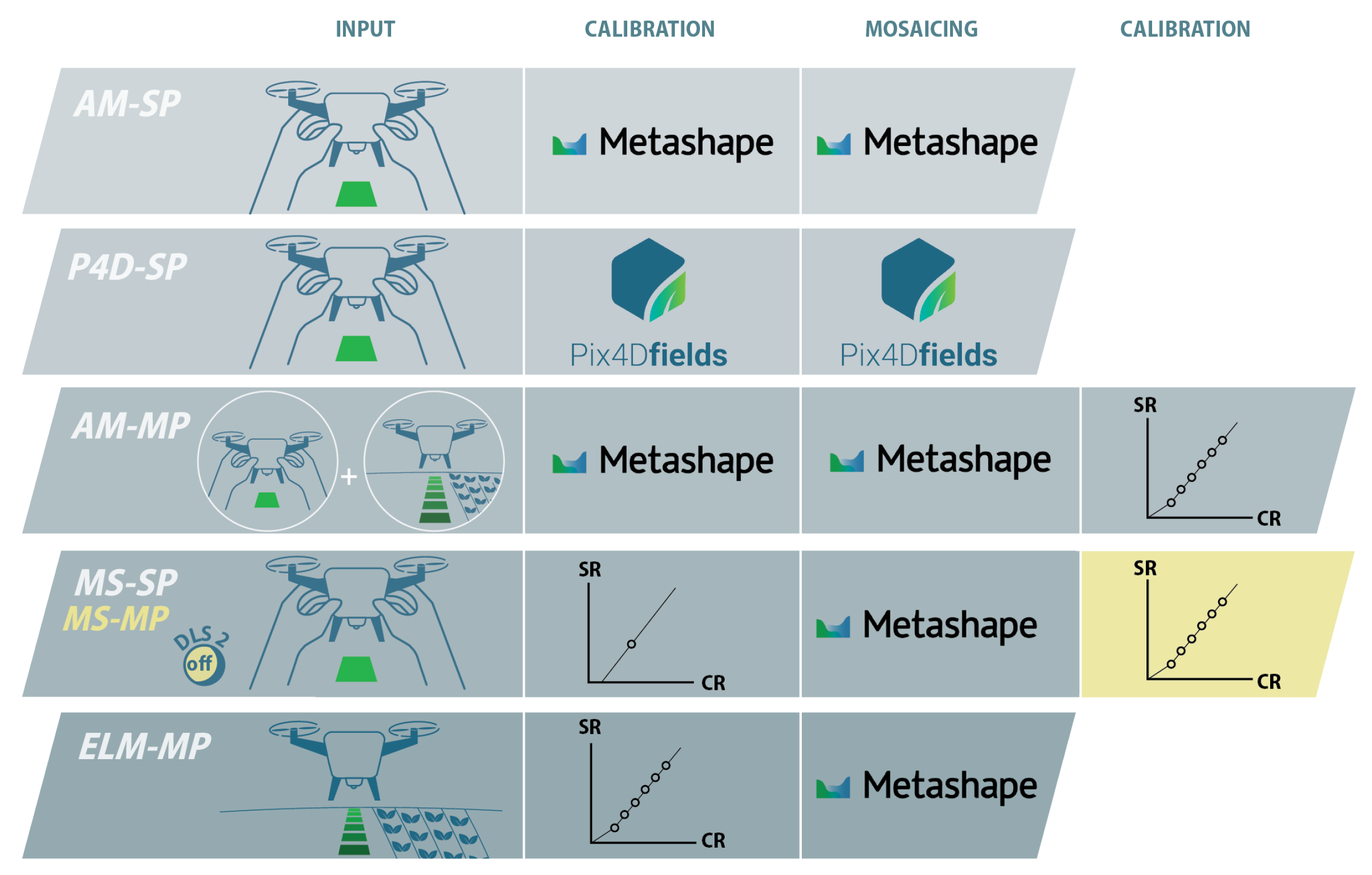
In this article, we compared the performance in radiometric calibration of the two most commonly used commercial software packages Pix4D Fields and Agisoft Metashape (P4D-SP and AM-SP methods), with those of more advanced methods. As mentioned in the introduction, the commercial software packages require less expert knowledge to convert raw images into usable reflectance maps compared to the other methods. The downsides of these solutions is that the user has little insight into or control over the process. In addition, our results show that differences exist in how both packages have implemented radiometric calibration, even though the raw datasets were identical, and both developers reference the same methods in their manuals [8,9].

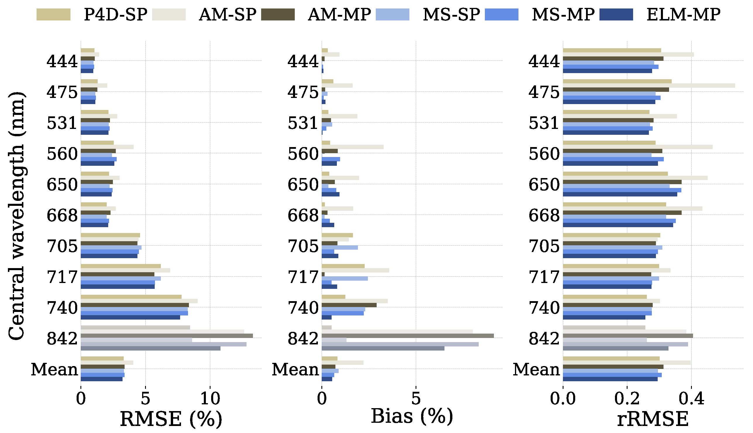
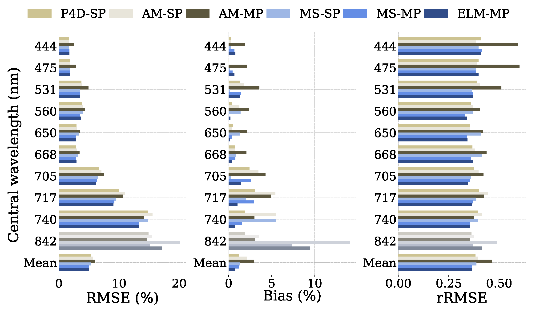
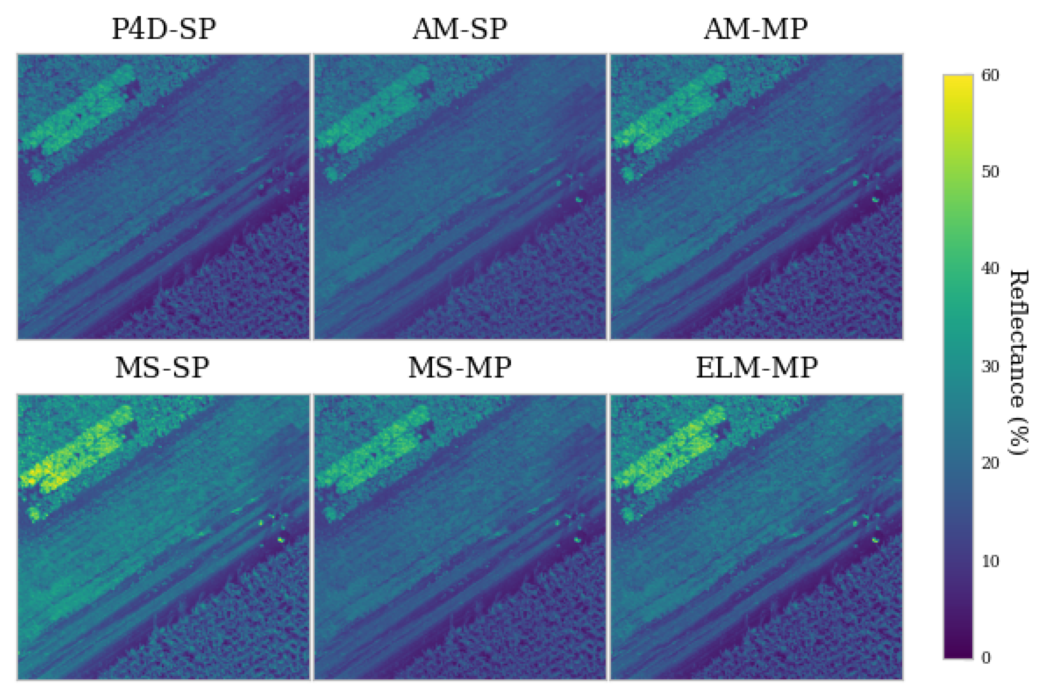
For both datasets, the AM-SP method clearly showed a higher bias than the P4D-SP method. The bias differences were consistent across the bands, except for the band at 705 nm, where the bias of the AM-SP method was lower than that of the P4D-SP method. It is, however, important to note that not just the calibration algorithm, but the mosaicing algorithm differs between both packages as well. Visually, slight displacements of pixels were noticeable between the orthophotos generated by Pix4D Fields and Metashape, explaining a portion of the difference in accuracy between both methods as well. However, as these displacements were of a scale of less than 1 pixel width (<3 cm), this effect will have been small. Our results suggest that Pix4D might currently be the overall better option out of the two packages regarding radiometric calibration. However, both packages are actively developed, and future updates could change this [30].

The ELM-MP method performed best out of the tested methods in both conditions regarding the RMSE and bias scores. This indicates that more elaborate calibration methods do in fact improve calibration accuracy because they are likely to account for more variables, and require less assumptions than simplified methods. For example, by using reference images of the RRTs taken at mission height, we can correct for scattering and absorption effects by the atmosphere on the optical path between the surface and the sensor. Our results indicate that this adds accuracy to the calibration workflow, at the cost of increased processing complexity. In our case, flight height was relatively low (29 m). We expect that the advantage of measuring RRTs from the dedicated mission height will increase with increasing flight altitudes, provided reference panels are large enough, or in conditions with more atmospheric scattering (e.g., presence of aerosols). Scattering and absorption effects are ignored when imaging a reference target at ground level, as was done for the P4D, AM and MS-SP methods. Another advantage is the use of multiple panels over just one. Multiple panels allow for the detection of saturation in the panels, as saturation would cause deviations from the linear relationship between at-sensor radiance and surface reflectance [35]. The use of multiple panels therefore adds accuracy at the cost of a more intensive workflow in the field.

Still, as mentioned, the difference between most methods is small. For most applications, the calibration results from Pix4D Fields would be adequately accurate, and the added value of using more complex calibration methods depends on the accuracy requirements of a given research question. Especially if vegetation indices are the intended end product, the more user-friendly solutions are suitable [42]. For more complex research questions involving analysis of individual bands, or when incorporating datasets from different locations or taken in different weather conditions, our study indicates that the ELM-MP method can lead to more reliable results.

One of the main sources of uncertainty within the P4D-SP, AM-SP and MS workflows is that the calibration panel needs to be imaged at ground level. Applying the ELM with the 6 gray RRTs on orthophotos that were generated using the single RRT was therefore hypothesized to improve accuracy. For the dataset in clear-sky conditions, applying an additional ELM correction to the orthophoto produced by the AM-SP method removes a large amount of bias for all bands except at 740 nm. This was expected, since corrections based on the gray RRTs are determined by an image taken by the UAV at mission height, and are assumed to be more accurate than the reference image at ground level. The ELM is especially fit for removing biases that may be present after the AM-SP method, since the added correction will be highly homogeneous over the entire orthophoto. The effect on the RMSE score will be limited since all samples are equally corrected. The results of the AM-MP method on the overcast dataset are however unexpected. There, the method added bias, instead of reducing it. A possible explanation for this lies in the way orthophotos are calculated. A given pixel in an orthophoto generated by Metashape is extracted from an individual image. During a mapping mission, the UAV usually makes multiple passes over the RRTs. It is therefore possible that there is a time gap between the spectrometer measurements of the RRTs and the used image(s) for the targets in the final orthophoto. When conditions are unstable, a large difference in incoming irradiance is possible as well. When applying the ELM on individual images, as in the ELM-MP method, it is possible to select a representative image of the reference targets near the same time as the spectrometer measurements.

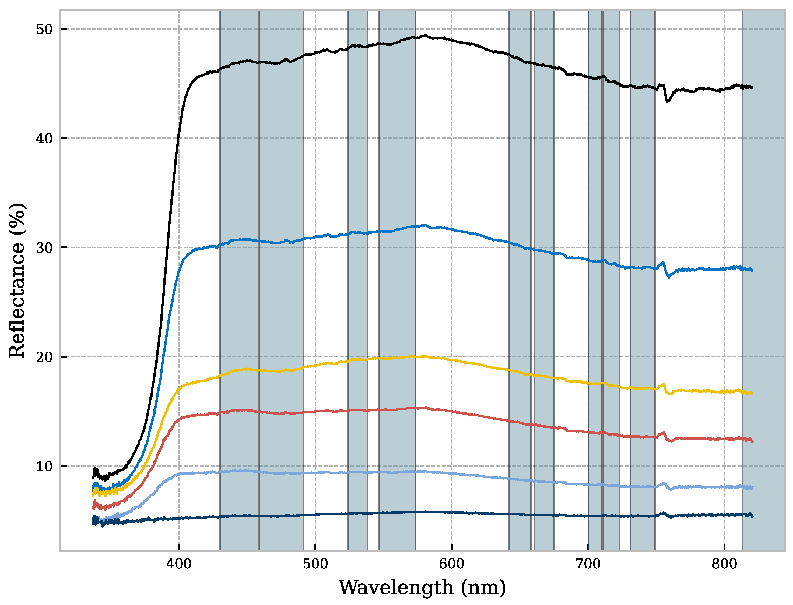
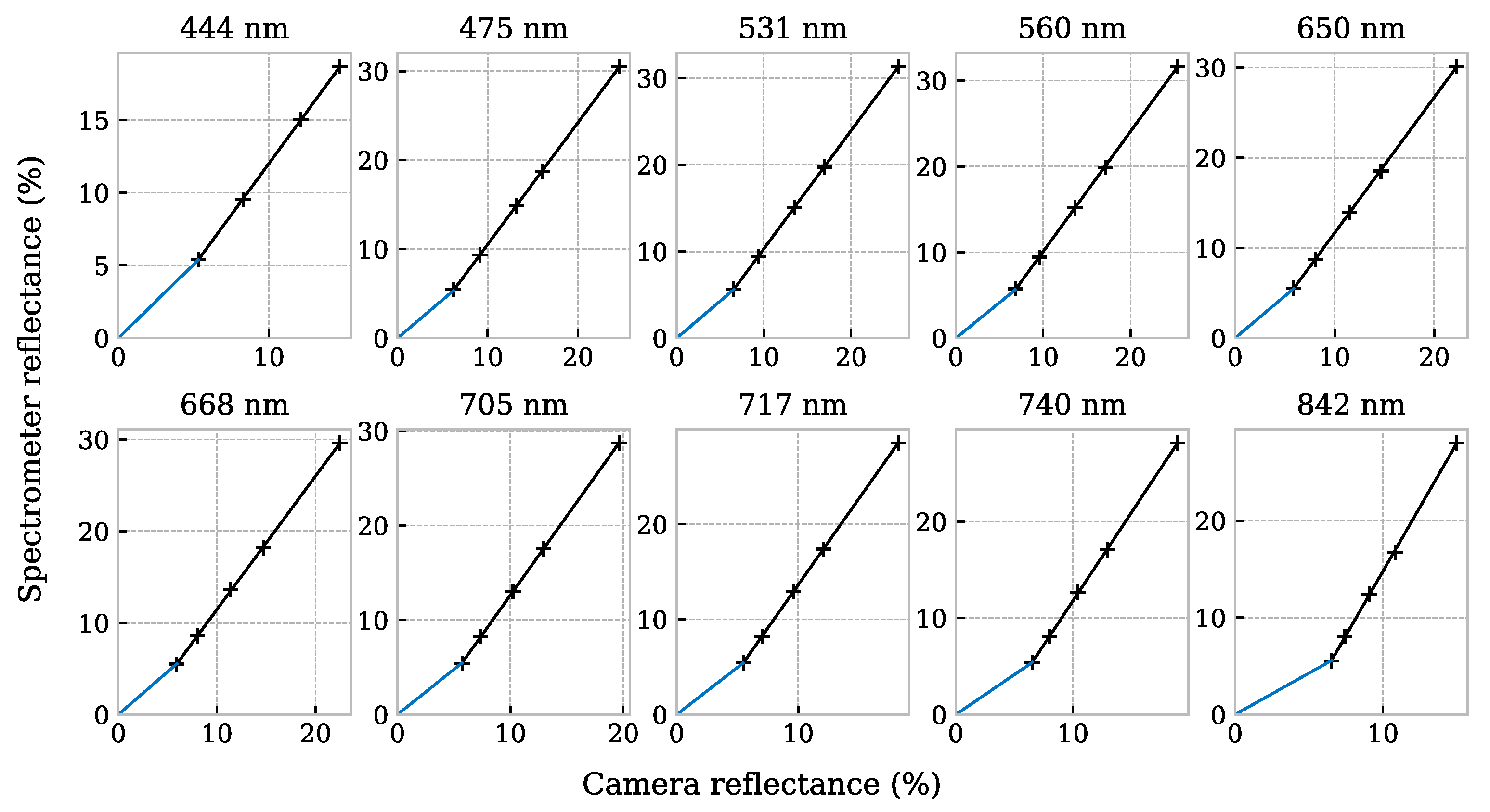
Baugh & Groeneveld (2007) showed that the relationship between remotely sensed DN and surface reflectance is in fact linear, and therefore calibrations should be reliable outside of the reflectance range of the RRTs [21]. Still, Aasen et al. (2018) recommended using targets that cover the expected reflectance range of the subject(s) of interest [18]. Our darkest RRT had an average reflectance of 5% (Figure 3), which was higher than the vegetation reflectance in the VIS spectrum (

Table A1. Fractions of pixels darker than the darkest gray reference target for the ELM-MP method.

Central Wavelength (nm)	444	475	531	560	650	668	705	717	740	842
Clear conditions	0.82	0.77	0.42	0.26	0.57	0.62	0.11	0.07	0.04	0.03
Overcast conditions	0.95	0.92	0.47	0.27	0.63	0.68	0.06	0.03	0.01	0.01

), and thus most of the area of interest fell outside of the RRTs’ reflectance range. Using a darker panel might therefore improve calibrations further.

For assessing the accuracy of radiometrically calibrated images, we used spectrometer measurements taken at ground level. Calibrating the spectrometer before a measurement took between 10 and 20 s. In overcast conditions, this time window is enough for the irradiance to change substantially during the measurement process, or otherwise affect the sensor calibration or measurement [43], while care was taken to avoid measurements during periods of noticeably varying irradiation, it is impossible to be certain that varying irradiance did not affect ground truth measurements, which might explain part of the added RMSE and bias in overcast conditions, compared to clear-sky conditions. Additionally, this reasoning is valid for the measurements of the gray RRTs as well, possibly affecting the calibration procedure itself. A possible improvement for this workflow would be to use an irradiance sensor at ground level and correct the reference spectrometer measurements for changes in solar irradiance.

It is well known that cloud coverage alters the irradiance spectrum [44]. This has biological implications, as plant reflectance changes with varying cloud coverage [45]. This should be taken into account when comparing the datasets from overcast and clear-sky conditions. More recently, Mamaghani et al. (2019) showed that the reflectance of plants is less variable in overcast than in clear-sky conditions, likely due to an increased influence of shadows within the canopy in direct light conditions [46,47,48]. Because of this, they recommend taking images in overcast or diffuse light conditions and using GSDs of 8 cm or higher, and found that the absolute radiometric correction workflow was sufficiently accurate. These results were obtained in a stationary setup with a Micasense RedEdge-3 camera. In our case, radiometric corrections in overcast conditions were less reliable than in clear-sky conditions. Therefore, we do not recommend following the advice given by Mamaghani et al. when applying any of the radiometric calibration methods tested in this study for UAV missions, unless a very reliable method can be developed for radiometric calibration.

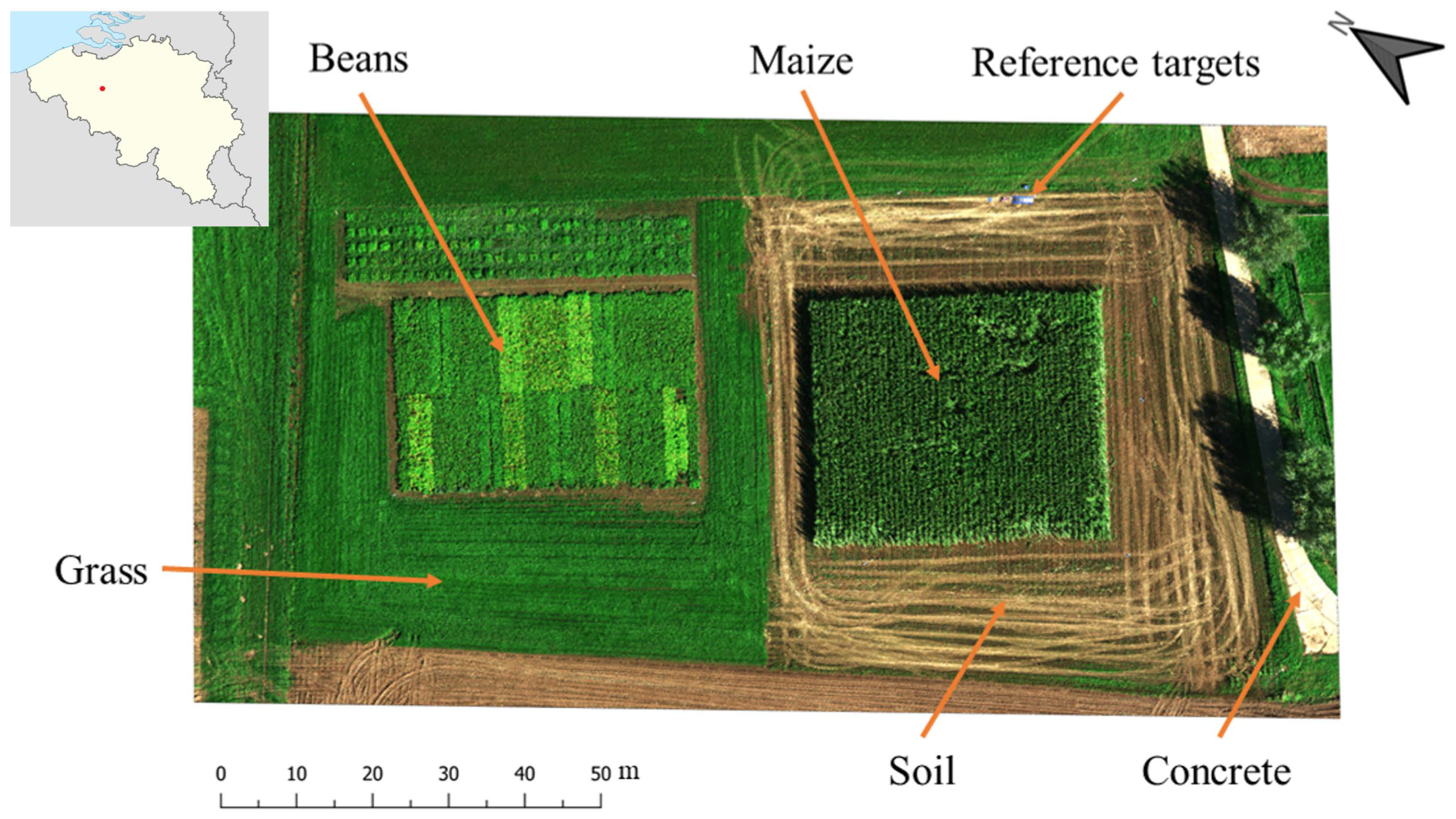
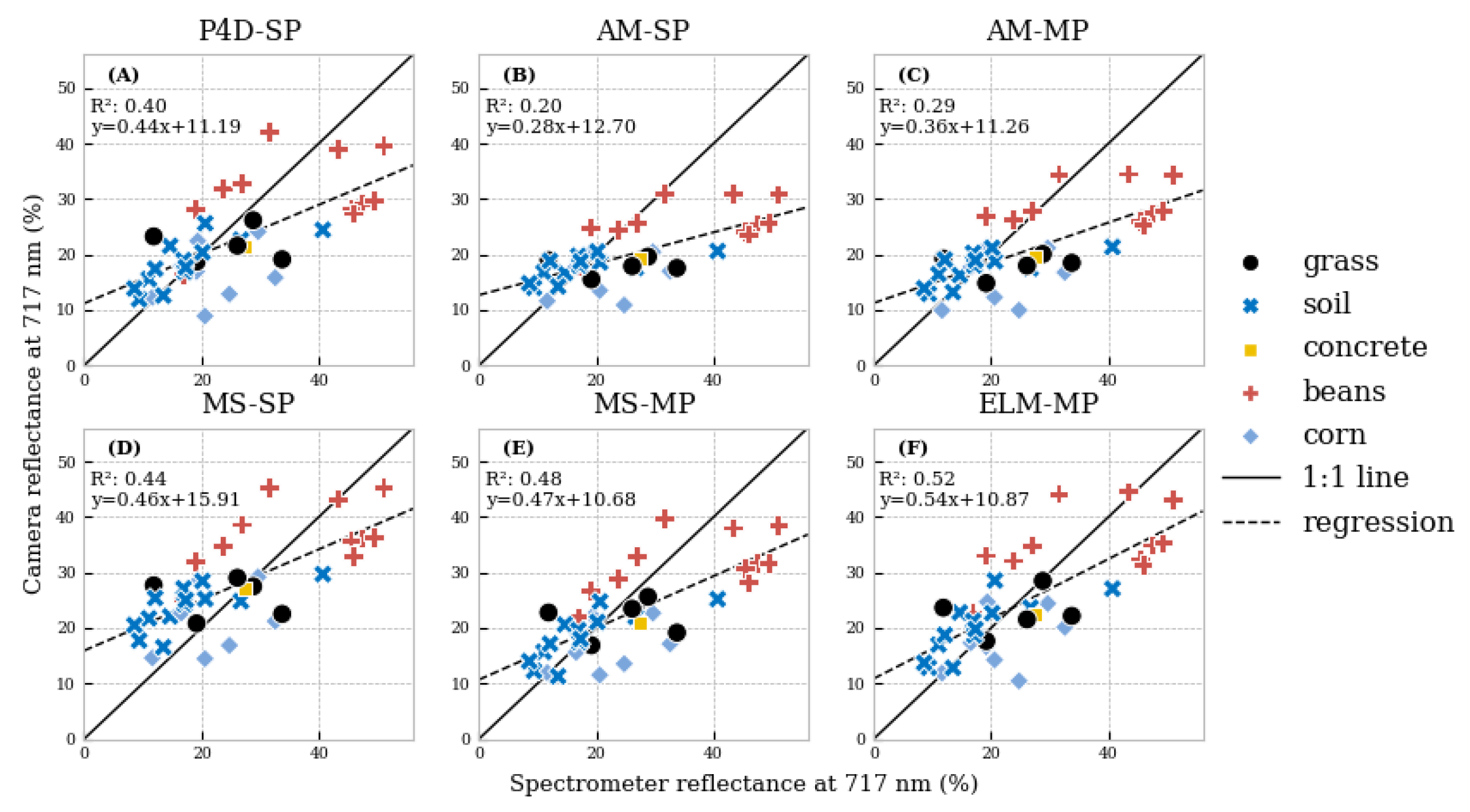
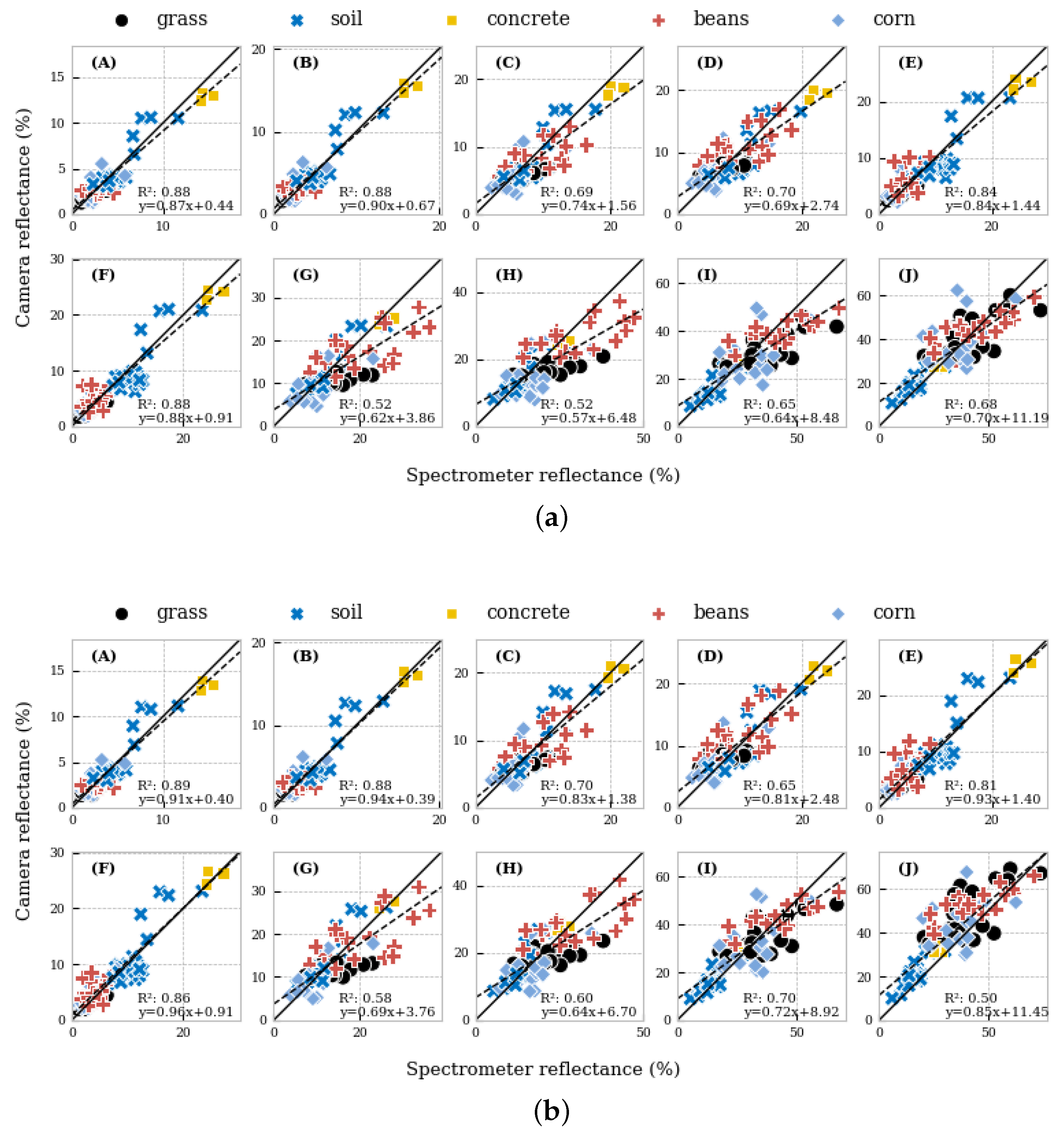
The different land cover classes were chosen to have a large range of intensities across the spectrum in our datasets (Figure 11). The plant classes (beans, corn and grass) showed higher relative variations, due to them moving in the wind and the constantly changing shadows within the canopies. Shadow correction techniques could reduce these effects and make the method more reliable [49,50].

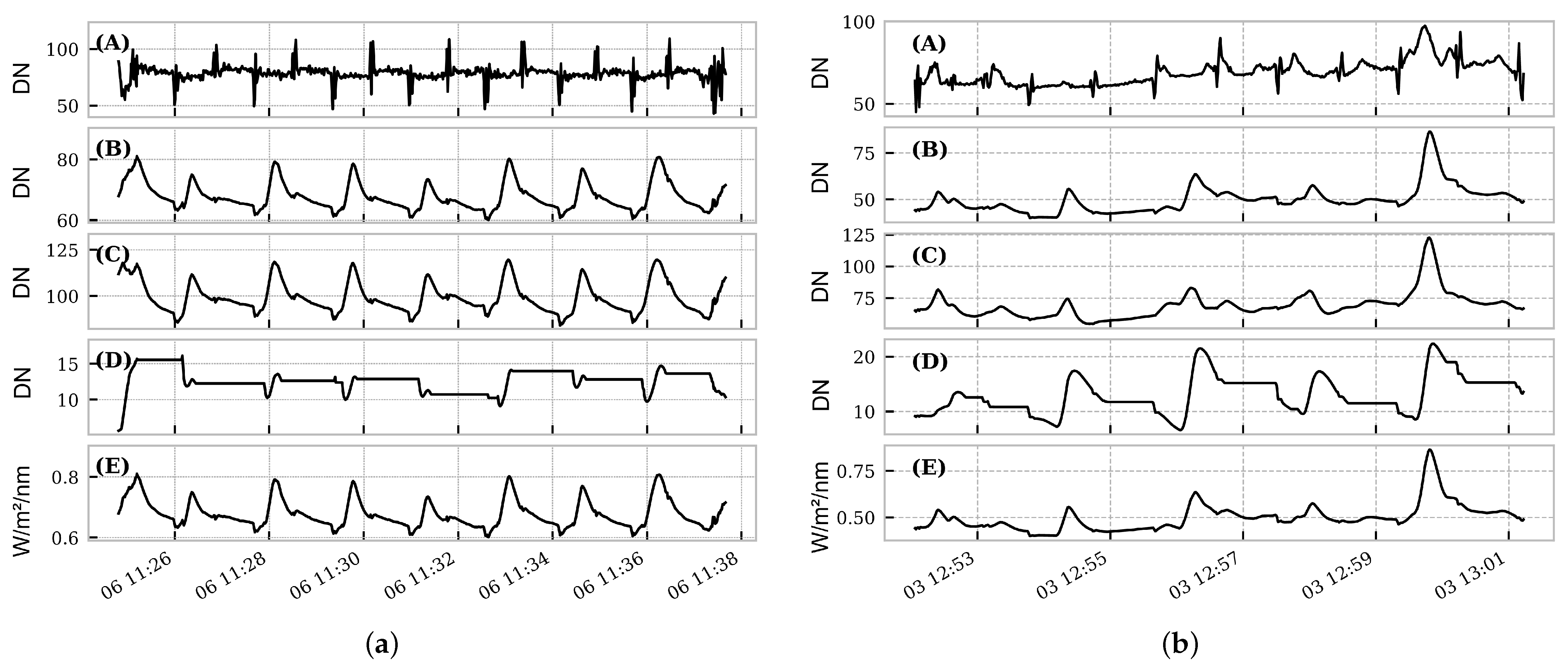
The AM-SP, MS and ELM-MP methods unexpectedly performed better when DLS2 corrections were disabled in overcast conditions. Clearly, the sensor is highly sensitive to orientation with respect to the sun. Correspondence with MicaSense revealed that these fluctuations are expected in stable weather conditions, and disabling DLS2 corrections in such cases is the recommended practice. A method for correcting the raw DLS2 measurements is proposed on the MicaSense GitHub page, but as Figure 7 shows, it was not able to remove the orientation effect. A better correction for relative tilt of the DLS2 measurements could lead to an improvement in accuracy [51]. However, the specifics behind the different irradiance parameters in the image metadata are not disclosed, so they would need empirical determination. Alternatively, the recent development of illumination estimation techniques without irradiance sensors, based on image keypoints found during the photogrammetry process, could improve the results further as well [37,47,48].

Our hardware setup might also have induced some inaccuracies. It is recommended by MicaSense to ensure that the up-welling radiance (the camera) and down-welling radiance (the DLS2 sensor) sensors are always at a reciprocal angle [18]. However, in our setup, the camera was mounted on a gimbal, making sure each image was taken pointing nadir. Because of this, we could not use more accurate viewing angles determined during image stitching in photogrammetry software, and had to rely on the likely less accurate IMU sensor of the DLS2. A solution could be to mount the irradiance sensor on a high precision gimbal.

The resampling of hyperspectral ground measurements was done based on the available spectral information of the camera, namely central wavelengths and bandwidths. Ideally, this should be done by convolving the spectral response curves over the hyperspectral measurements, as sensors are not equally sensitive to each wavelength within a given band range [15]. However, this was not possible as the spectral response curves of our camera are not disclosed by the manufacturer, and we did not have access to specialized equipment to determine the response curves ourselves.

During the processing, we did not account for bidirectional reflectance distribution function (BRDF) effects or other scene reflectance effects like shadow or topography corrections on the surface reflectance for several reasons. The main reason being that we wanted to focus on the radiometric calibration process itself. As these scene reflectance corrections would influence the intermediary result, comparing different methods would become more challenging. Furthermore, the commercial solutions Pix4D Fields and Agisoft Metashape do not include these corrections in their workflow, so methods that do include BRDF corrections would have an advantage, assuming the corrections are accurate. An optimal calibration workflow would include such corrections, if they are sufficiently reliable. This reliability is likely to depend on flight conditions.

While our study focused on a specific multispectral camera, our results concerning the use of multiple radiometric reference targets, taking reference images at mission altitude and the effect of clouds on the reliability of reflectance maps can be extrapolated to other sensors. Several studies have determined the spectral consistencies between different multispectral sensors [52,53,54], while good correlations between the raw images of different sensors have been found, errors of 2–5% are expected, depending on the wavelength. Furthermore, the measuring altitude influences this error. This emphasizes the importance of good radiometric calibrations.

6. Conclusions

The radiometric calibration of remotely sensed images is an ongoing topic in the RS community. Several different approaches have been proposed for correcting images for effects due to the environment that alter the measured signals. Since it is hard to compare them based on readily available information, we have performed an empirical comparison of 5 different commonly used implementations in clear-sky and overcast conditions for the MicaSense MX Dual Camera System. These methods were compared based on the RMSE and bias scores from calibrated pixels compared to ground level spectrometer measurements of different targets. Out of two commercial products, Pix4D Fields produced slightly better results, especially in clear-sky conditions. However, we showed that using multiple panels for applying the ELM on individual images, and taking the reference image from the same altitude as the rest of the mission (ELM-MP method) resulted in even more accurate calibrations. The drawback is that this is a much more involved method, both to apply in the field and in the processing stage. In many cases, the commercial user-friendly methods, like the ones offered by Metashape and Pix4D, might be ’good enough’. Next, our results confirm that flying in clear-sky conditions is preferable over unstable conditions, independent of the used calibration method. Although, in unstable conditions, we found that the ELM-MP method had a larger added value than in stable conditions. To conclude, we argue that the choice of the calibration method depends on, required accuracy, time constraints and flight conditions. When time is of the essence and results are needed fast, the simplified ELM is by far the fastest method and can be executed semi-automatically in commercially available software. In overcast conditions or when accuracy is of great importance, we recommend more elaborate calibration methods like our ELM-MP method.

References

1. Maes, W.H.; Steppe, K. Perspectives for Remote Sensing with Unmanned Aerial Vehicles in Precision Agriculture. Trends Plant Sci. 2019, 24, 152–164. [Google Scholar] [CrossRef]
2. Colomina, I.; Molina, P. Unmanned aerial systems for photogrammetry and remote sensing: A review. ISPRS J. Photogramm. Remote Sens. 2014, 92, 79–97. [Google Scholar] [CrossRef] [Green Version]
3. Perich, G.; Meyer, P.; Wieser, A.; Liebisch, F. Proximal and Drone Based Hyperspectral Sensing for Crop Nitrogen Status Detection in Historic Field Trials. In Proceedings of the Workshop on Hyperspectral Image and Signal Processing, Evolution in Remote Sensing, Amsterdam, The Netherlands, 24–26 March 2021. [Google Scholar] [CrossRef]
4. Maimaitijiang, M.; Ghulam, A.; Sidike, P.; Hartling, S.; Maimaitiyiming, M.; Peterson, K.; Shavers, E.; Fishman, J.; Peterson, J.; Kadam, S.; et al. Unmanned Aerial System (UAS)-based phenotyping of soybean using multi-sensor data fusion and extreme learning machine. ISPRS J. Photogramm. Remote Sens. 2017, 134, 43–58. [Google Scholar] [CrossRef]
5. Weiss, M.; Jacob, F.; Duveiller, G. Remote sensing for agricultural applications: A meta-review. Remote Sens. Environ. 2020, 236, 111402. [Google Scholar] [CrossRef]
6. Aasen, H.; Bolten, A. Multi-temporal high-resolution imaging spectroscopy with hyperspectral 2D imagers—From theory to application. Remote Sens. Environ. 2018, 205, 374–389. [Google Scholar] [CrossRef]
7. Walker, S.E.; Sheaves, M.; Waltham, N.J. Barriers to Using UAVs in Conservation and Environmental Management: A Systematic Review. Environ. Manag. 2022, 71, 1052–1064. [Google Scholar] [CrossRef] [PubMed]
8. Pix4D. Radiometric Corrections; JIYI Robotics Co.: Shanghai, China, 2020. [Google Scholar]
9. Agisoft. Agisoft Metashape: User Manuals; Agisoft LLC: St. Petersburg, Russia, 2023. [Google Scholar]
10. MicaSense. Radiometric Calibration Model for MicaSense Sensors; MicaSense Inc.: Seattle, WA, USA, 2022. [Google Scholar]
11. Tmušić, G.; Manfreda, S.; Aasen, H.; James, M.R.; Gonçalves, G.; Ben-Dor, E.; Brook, A.; Polinova, M.; Arranz, J.J.; Mészáros, J.; et al. Current practices in UAS-based environmental monitoring. Remote Sens. 2020, 12, 1001. [Google Scholar] [CrossRef] [Green Version]
12. Pell, T.; Li, J.Y.; Joyce, K.E. Demystifying the Differences between Structure-from-MotionSoftware Packages for Pre-Processing Drone Data. Drones 2022, 6, 24. [Google Scholar] [CrossRef]
13. Honkavaara, E.; Khoramshahi, E. Radiometric Correction of Close-Range Spectral Image Blocks Captured Using an Unmanned Aerial Vehicle with a Radiometric Block Adjustment. Remote Sens. 2018, 10, 256. [Google Scholar] [CrossRef] [Green Version]
14. Li, W.; Sun, K.; Li, D.; Bai, T. Algorithm for automatic image dodging of unmanned aerial vehicle images using two-dimensional radiometric spatial attributes. J. Appl. Remote Sens. 2016, 10, 036023. [Google Scholar] [CrossRef] [Green Version]
15. Mamaghani, B.; Salvaggio, C. Multispectral Sensor Calibration and Characterization for sUAS Remote Sensing. Sensors 2019, 19, 4453. [Google Scholar] [CrossRef] [Green Version]
16. Smith, G.M.; Milton, E.J. The use of the empirical line method to calibrate remotely sensed data to reflectance. Int. J. Remote Sens. 1999, 20, 2653–2662. [Google Scholar] [CrossRef]
17. Schowengerdt, R.A. Remote Sensing; Elsevier: Amsterdam, The Netherlands, 2006; pp. 1–515. [Google Scholar] [CrossRef]
18. Aasen, H.; Honkavaara, E.; Lucieer, A.; Zarco-Tejada, P.J. Quantitative remote sensing at ultra-high resolution with UAV spectroscopy: A review of sensor technology, measurement procedures, and data correctionworkflows. Remote Sens. 2018, 10, 1091. [Google Scholar] [CrossRef] [Green Version]
19. Jiang, J.; Johansen, K.; Tu, Y.H.; McCabe, M.F. Multi-sensor and multi-platform consistency and interoperability between UAV, Planet CubeSat, Sentinel-2, and Landsat reflectance data. GISci. Remote Sens. 2022, 59, 936–958. [Google Scholar] [CrossRef]
20. Pozo, S.D.; Rodríguez-Gonzálvez, P.; Hernández-López, D.; Felipe-García, B. Vicarious Radiometric Calibration of a Multispectral Camera on Board an Unmanned Aerial System. Remote Sens. 2014, 6, 1918–1937. [Google Scholar] [CrossRef] [Green Version]
21. Baugh, W.M.; Groeneveld, D.P. Empirical proof of the empirical line. Int. J. Remote Sens. 2007, 29, 665–672. [Google Scholar] [CrossRef]
22. Cubero-Castan, M.; Schneider-Zapp, K.; Bellomo, M.; Shi, D.; Rehak, M.; Strecha, C. Assessment of the Radiometric Accuracy in A Target Less Work Flow Using Pix4D Software. In Proceedings of the Workshop on Hyperspectral Image and Signal Processing, Evolution in Remote Sensing, Amsterdam, The Netherlands, 23–26 September 2018. [Google Scholar] [CrossRef]
23. Schneider-Zapp, K.; Cubero-Castan, M.; Shi, D.; Strecha, C. A new method to determine multi-angular reflectance factor from lightweight multispectral cameras with sky sensor in a target-less workflow applicable to UAV. Remote Sens. Environ. 2019, 229, 60–68. [Google Scholar] [CrossRef] [Green Version]
24. Zhou, X.; Liu, C.; Xue, Y.; Akbar, A.; Jia, S.; Zhou, Y.; Zeng, D. Radiometric calibration of a large-array commodity CMOS multispectral camera for UAV-borne remote sensing. Int. J. Appl. Earth Obs. Geoinf. 2022, 112, 102968. [Google Scholar] [CrossRef]
25. Bendig, J.; Gautam, D.; Malenovský, Z.; Lucieer, A. Influence of cosine corrector and UAS platform dynamics on airborne spectral irradiance measurements. In Proceedings of the GARSS 2018—2018 IEEE International Geoscience and Remote Sensing Symposium, Valencia, Spain, 22–27 July 2018; pp. 8822–8825. [Google Scholar] [CrossRef]
26. Suomalainen, J.; Hakala, T.; de Oliveira, R.A.; Markelin, L.; Viljanen, N.; Näsi, R.; Honkavaara, E. A Novel Tilt Correction Technique for Irradiance Sensors and Spectrometers On-Board Unmanned Aerial Vehicles. Remote Sens. 2018, 10, 2068. [Google Scholar] [CrossRef] [Green Version]
27. Padró, J.C.; Muñoz, F.J.; Ávila, L.Á.; Pesquer, L.; Pons, X. Radiometric correction of Landsat-8 and Sentinel-2A scenes using drone imagery in synergy with field spectroradiometry. Remote Sens. 2018, 10, 1687. [Google Scholar] [CrossRef] [Green Version]
28. Padró, J.C.; Carabassa, V.; Balagué, J.; Brotons, L.; Alcañiz, J.M.; Pons, X. Monitoring opencast mine restorations using Unmanned Aerial System (UAS) imagery. Sci. Total. Environ. 2019, 657, 1602–1614. [Google Scholar] [CrossRef]
29. Wang, C.; Myint, S.W. A Simplified Empirical Line Method of Radiometric Calibration for Small Unmanned Aircraft Systems-Based Remote Sensing. IEEE J. Sel. Top. Appl. Earth Obs. Remote Sens. 2015, 8, 1876–1885. [Google Scholar] [CrossRef]
30. Di Gennaro, S.F.; Toscano, P.; Gatti, M.; Poni, S.; Berton, A.; Matese, A. Spectral Comparison of UAV-Based Hyper and Multispectral Cameras for Precision Viticulture. Remote Sens. 2022, 14, 449. [Google Scholar] [CrossRef]
31. Abdelbaki, A.; Schlerf, M.; Retzlaff, R.; Machwitz, M.; Verrelst, J.; Udelhoven, T. Comparison of Crop Trait Retrieval Strategies Using UAV-Based VNIR Hyperspectral Imaging. Remote Sens. 2021, 13, 1748. [Google Scholar] [CrossRef]
32. Cao, H.; Gu, X.; Wei, X.; Yu, T.; Zhang, H. Lookup Table Approach for Radiometric Calibration of Miniaturized Multispectral Camera Mounted on an Unmanned Aerial Vehicle. Remote Sens. 2020, 12, 4012. [Google Scholar] [CrossRef]
33. Poncet, A.M.; Knappenberger, T.; Brodbeck, C.; Fogle, M.; Shaw, J.N.; Ortiz, B.V. Multispectral UAS data accuracy for different radiometric calibration methods. Remote Sens. 2019, 11, 1917. [Google Scholar] [CrossRef] [Green Version]
34. Tu, Y.H.; Phinn, S.; Johansen, K.; Robson, A. Assessing Radiometric Correction Approaches for Multi-Spectral UAS Imagery for Horticultural Applications. Remote Sens. 2018, 10, 1684. [Google Scholar] [CrossRef] [Green Version]
35. Dao, P.D.; He, Y.; Lu, B. Maximizing the quantitative utility of airborne hyperspectral imagery for studying plant physiology: An optimal sensor exposure setting procedure and empirical line method for atmospheric correction. Int. J. Appl. Earth Obs. Geoinf. 2019, 77, 140–150. [Google Scholar] [CrossRef]
36. Svensgaard, J.; Jensen, S.M.; Christensen, S.; Rasmussen, J. The importance of spectral correction of UAV-based phenotyping with RGB cameras. Field Crop. Res. 2021, 269, 108177. [Google Scholar] [CrossRef]
37. Qin, Z.; Li, X.; Gu, Y. An Illumination Estimation and Compensation Method for Radiometric Correction of UAV Multispectral Images. IEEE Trans. Geosci. Remote Sens. 2022, 60, 5545012. [Google Scholar] [CrossRef]
38. Visual Crossing. Weather Data Services|Visual Crossing; Visual Crossing: Herndon, VA, USA, 2023. [Google Scholar]
39. Micasense Image. Micasense Image Processing Tutorials; MicaSense Inc.: Seattle, WA, USA, 2019. [Google Scholar]
40. Pix4D. PIX4Dfields—Support; JIYI Robotics Co.: Shanghai, China, 2023. [Google Scholar]
41. QGIS. QGIS User Guide—QGIS Documentation Documentation; Geospatial Foundation: Herndon, VA, USA, 2023. [Google Scholar]
42. Olsson, P.O.; Vivekar, A.; Adler, K.; Garcia Millan, V.E.; Koc, A.; Alamrani, M.; Eklundh, L. Radiometric Correction of Multispectral UAS Images: Evaluating the Accuracy of the Parrot Sequoia Camera and Sunshine Sensor. Remote Sens. 2021, 13, 577. [Google Scholar] [CrossRef]
43. Chang, J.; Clay, S.A.; Clay, D.E.; Aaron, D.; Helder, D.; Dalsted, K. Clouds Influence Precision and Accuracy of Ground-Based Spectroradiometers. Commun. Soil Sci. Plant Anal. 2007, 36, 1799–1807. [Google Scholar] [CrossRef]
44. Bartlett, J.S.; Ciotti, A.M.; Davis, R.F.; Cullen, J.J. The spectral effects of clouds on solar irradiance. J. Geophys. Res. Ocean. 1998, 103, 31017–31031. [Google Scholar] [CrossRef]
45. Tumbo, S.D.; Wagner, D.G.; Heinemann, P.H. Hyperspectral characteristics of corn plants under different chlorophyll levels. Trans. Am. Soc. Agric. Eng. 2002, 45, 815–823. [Google Scholar] [CrossRef]
46. Mamaghani, B.; Saunders, M.G.; Salvaggio, C. Inherent Reflectance Variability of Vegetation. Agriculture 2019, 9, 246. [Google Scholar] [CrossRef] [Green Version]
47. Moghimi, A.; Celik, T.; Mohammadzadeh, A.; Kusetogullari, H. Comparison of Keypoint Detectors and Descriptors for Relative Radiometric Normalization of Bitemporal Remote Sensing Images. IEEE J. Sel. Top. Appl. Earth Obs. Remote Sens. 2021, 14, 4063–4073. [Google Scholar] [CrossRef]
48. Moghimi, A.; Celik, T.; Mohammadzadeh, A. Tensor-based keypoint detection and switching regression model for relative radiometric normalization of bitemporal multispectral images. Int. J. Remote Sens. 2022, 43, 3927–3956. [Google Scholar] [CrossRef]
49. Pons, X.; Padró, J.C. An empirical approach on shadow reduction of uav imagery in forests. In Proceedings of the International Geoscience and Remote Sensing Symposium (IGARSS), Yokohama, Japan, 28 July–2 August 2019; Volume 201, pp. 2463–2466. [Google Scholar] [CrossRef]
50. Pons, X.; Padró, J.C. An operational radiometric correction technique for shadow reduction in multispectral uav imagery. Remote Sens. 2021, 13, 3808. [Google Scholar] [CrossRef]
51. Köppl, C.J.; Malureanu, R.; Dam-Hansen, C.; Wang, S.; Jin, H.; Barchiesi, S.; Serrano Sandí, J.M.; Muñoz-Carpena, R.; Johnson, M.; Durán-Quesada, A.M.; et al. Hyperspectral reflectance measurements from UAS under intermittent clouds: Correcting irradiance measurements for sensor tilt. Remote Sens. Environ. 2021, 267, 112719. [Google Scholar] [CrossRef]
52. Franzini, M.; Ronchetti, G.; Sona, G.; Casella, V. Geometric and radiometric consistency of parrot sequoia multispectral imagery for precision agriculture applications. Appl. Sci. 2019, 9, 5314. [Google Scholar] [CrossRef] [Green Version]
53. Lu, H.; Fan, T.; Ghimire, P.; Deng, L. Experimental Evaluation and Consistency Comparison of UAV Multispectral Minisensors. Remote Sens. 2020, 12, 2542. [Google Scholar] [CrossRef]
54. Kasimati, A.; Psiroukis, V.; Darra, N.; Kalogrias, A.; Kalivas, D.; Taylor, J.A.; Fountas, S. Investigation of the similarities between NDVI maps from different proximal and remote sensing platforms in explaining vineyard variability. Precis. Agric. 2023, 1–21. [Google Scholar] [CrossRef]
Figure 1. Overview of the experimental site at 50°57′29.1″N 3°46′00.9″E.
Remotesensing 15 02909 g001
Figure 2. Left: white reference panel captured in band 5 (642 nm–658 nm) of the MicaSense dual camera system. Right: Aerial image of the 6 RRTs captured in band 2 (459 nm–491 nm).
Remotesensing 15 02909 g002
Figure 3. Spectrometer measurements for the six gray RRTs used for corrections on 6 October. The gray bands indicate the multispectral bands of the camera. The spectrometer was calibrated using a Spectralon 99% reflectance panel before each measurement.
Remotesensing 15 02909 g003
Figure 4. Schematic representation of the 5 different methods. The inputs, calibration methods and mosaicing methods are shown. The graphs depicting the ELM with one or 6 reference targets are shown with surface reflectance (SR) on the Y-axis and camera reflectance (CR) on the X-axis. Calibrations before mosaicing were done at image-level, after mosaicing, calibrations were done on the orthomosaic.
Remotesensing 15 02909 g004
Figure 5. Overview of the workflow for calibrating multispectral images using the ELM-MP method. Rectangles depict processing steps, slanted rectangles depict inputs, trapeziums depict manual steps in the workflow and rounded shapes depict the output.
Remotesensing 15 02909 g005
Figure 6. Illustration of the two linear models for each band used for describing the relationship between at-sensor radiance and surface reflectance.
Remotesensing 15 02909 g006
Figure 7. Irradiance measured by the DLS2 sensor during the flight on 6 October (a) and 3 October (b). The temporal profile of the measurements was very similar for all bands of the camera for each flight. (A): Spectral irradiance, (B): Horizontal irradiance, (C): Direct irradiance, (D): Scattered irradiance, (E): Corrected irradiance. (a) Sunny; (b) Overcast.
Remotesensing 15 02909 g007
Figure 8. RMSE, bias and rRMSE comparison between the different methods on the dataset captured in clear-sky conditions. P4D-SP: Pix4D calibration, AM-SP: Metashape calibration, AM-MP: Metashape with empirical line correction on orthophoto, MS: single panel correction, MP: multiple panel correction. The mean was calculated without band 10 (842 nm).
Remotesensing 15 02909 g008
Figure 9. RMSE, bias and rRMSE comparison between the different methods on the dataset captured in overcast conditions. P4D-SP: Pix4D calibration, AM-SP: Metashape calibration, AM-MP: Metashape with empirical line correction on orthophoto, MS: single panel correction, MP: multiple panel correction.
Remotesensing 15 02909 g009
Figure 10. Detail image of band 8 (717 nm) showing slight color differences between the calibration methods. The depicted area shows the edge of the beans (top left) and corn (bottom right) plots with grass in between.
Remotesensing 15 02909 g010
Figure 11. Scatterplot of the different land covers for band 8 (717 nm) for the overcast dataset. (A): P4D-SP method, (B): AM-SP method, (C): AM-MP method, (D): MS-SP method, (E): MS-MP method, (F): ELM-MP method.
Remotesensing 15 02909 g011