Examining the Consistency of Sea Surface Temperature and Sea Ice Concentration in Arctic Satellite Products

Abstract

Available observations and a theoretical simulation are used to explore the consistency and relationship between sea surface temperature (SST) and sea ice concentration (SIC) within open-ocean-sea ice mixed satellite pixels as a function of grid resolution. The maximum limiting SST value for a specified SIC and spatial resolution is first examined within collocated satellite-derived products contained within existing Level 4 SST analyses distributed using the data specification from the Group for High Resolution Sea Surface Temperature. The shape of the interdependence is further validated with manually quality-controlled buoy SST and SIC collocations. A parametric equation for the limiting SST value is derived from simulations of a mixed ocean/ice pixel with specified ice fraction and a linear SST gradient extending away from the ice edge. The exponential curve matching the observed interdependence suggests a maximum 5 km pixel-averaged SST at SIC values approaching zero between 6 and 8 °C. This maximum value is significantly greater than the previously assumed limiting values of ~3 °C and the corresponding SST gradient is larger than those typically observed with satellite SST products, but agrees well with recent Saildrone SST observations near ice. The curve provides a conservative limit with which inconsistent SST/SIC pairings can be identified, not only near the ice edge but at intermediate ice concentrations. Application of the filter improves the agreement between the SST/SIC relationship in satellite products and available Saildrone observations as well as the internal consistency of the different satellite products.

1. Introduction

The focus of this paper is on the consistency of satellite sea surface temperature (SST) and sea ice concentration (SIC) products during the Arctic sea ice melt season when the traditionally frozen sea ice cover can be viewed as a matrix of patches of ice and open water. High latitude (HL, >50 N/S latitude) satellite-derived “level 4” (L4) SST analyses are derived by merging multiple sources (e.g., satellite thermal infrared (IR), satellite passive microwave (MW), and in situ data) and mapping onto spatially complete grids. They also make use of independent MW satellite-derived sea ice concentration (SIC) analyses (complete maps of percent areal coverage of ice within a grid cell or pixel), regridded to the L4 SST grid, to flag pixels that may contain sea ice. To accurately establish the presence of sea ice within a common grid is an important step in the generation of HL L4 SST products, as analysis systems usually compute an SST value only where the corresponding SIC < ~50–55%. Where SIC > 50%, the SST analysis systems commonly relax the temperature of the pixel towards, or hold it fixed at, the freezing temperature of sea water (−1.8 °C or 271 K for a salinity of 33 psu). On occasions, however, the SIC analysis indicates the potential presence of sea ice (SIC > 0), when in reality the ocean surface is ice-free (SIC = 0%) or, vice-versa, the SIC product is set to zero suggesting that the ocean surface is free of ice when in fact it is not. These erroneous ice retrievals have been referred to as “SIC inconsistencies” by the SST community and are known by other names such as “false/spurious ice” by the SIC community (e.g., [1,2]). Because in most cases the SIC product used to flag the ice is produced externally from the SST analysis system, the question arises as to whether there are feedbacks between uncertainties in each of the products, and more specifically, whether the SIC inconsistencies have a negative impact on the analyzed SSTs.

Satellite SIC products traditionally use a combination of high and low frequency observations from sensors including SMMR, SSM/I, SSMIS, AMSR-E, and AMSR2. The full description of the acronyms used in the text to denote the satellite product-related terms is given in the Glossary. It is not the purpose of this paper to give an in-depth review of current SIC algorithms and related uncertainties. The reader is referred to the vast literature (e.g., [3,4,5]) for a comprehensive description of these issues. We are interested, instead, in characterizing the interdependence between SST and SIC for open water-sea ice mixed pixels in analyzed satellite products, especially when the surface temperature is close to the point of the phase change between open water and ice (i.e., near the ice edge).

Sea ice concentration retrievals are particularly problematic near the ice edge during the summer melt season (e.g., [6]). Sea ice misclassifications in satellite SIC products often result from multiple factors including active weather systems influencing the MW radiances, radiances from land in the MW footprint near coastal boundaries, and misrepresentation errors introduced by multiple regridding of the MW channels to finer spatial resolutions for analysis and product dissemination. Weather-contaminated SIC retrievals are more prone to occur during the Arctic summer ice melting season (mid-March to mid-September) and in the vicinity of marginal ice zones where atmospheric contributions (e.g., total water vapor, cloud liquid water, wind-induced roughness over open water) appear more pronounced in the MW radiances against the low emissive background of the open ocean. As the ice concentration increases and the atmosphere becomes drier, the MW sensitivity to atmospheric effects decreases and surface emissivity variability (due to ice type, snow depth, etc.) becomes the dominant source of uncertainty in the consolidated winter ice pack. The reader is referred to [7] for a comprehensive sensitivity study of eight SIC algorithms to geophysical noise.

In order to mitigate the high density of inconsistencies near the ice edge or to eliminate residual atmospheric contributions to the MW radiances, SIC algorithms use appropriately named “weather filters”. The MW radiances at the 37 GHz channel (0.81-cm wavelength) have a greater sensitivity to heavy cloud cover (associated with intense rainfall) than the 18 GHz (1.7-cm wavelength), by a factor of ~4 [8]. Consequently, weather filters are commonly designed based on “gradient ratios” between two MW spectral channels of different sensitivity; if the gradient ratios are larger than some specified threshold, the SIC is set to zero to indicate open ocean [9]. Nonetheless, weather filters tend to lose discriminatory power at low ice concentrations (and/or thin ice), in calm wind conditions, or in heavy weather [3], and some amount of unscreened atmospheric noise will remain.

To minimize these instances, especially along the ice edge, some SIC analyses use additional post-processing filters. The most common of these is to reset ice concentrations less than or equal to 15%, a threshold range commonly associated with the “ice edge” according to the National Snow and Ice Data Center, to SIC = 0%, i.e., to “open water”. For this reason, this type of inconsistency filtering is also known as the “open water filter” or OWF (e.g., [10]). Choosing to “delineate the ice edge” at the 10–15% ice concentration isopleth in order to minimize spurious ice retrievals in the ice margin, will come at the cost of losing the very low ice concentrations. Physically based corrections of the atmospheric contribution to the radiances have also been proposed as an alternative to the weather filtering approach (e.g., [3,5]). These are typically based on satellite or numerical weather prediction (NWP) estimates of atmospheric variables combined with a radiative transfer model (RTM), and are evaluated prior to the SIC algorithm at the brightness temperature (Tb)-level.

Sea ice concentration products have inherent spatial resolutions of the order of 50–60 km due to the footprint of traditional lower frequency MW channels (19 and 37 GHz) used in SIC algorithms (see, e.g., [3,5], and references therein). Improved spatial resolutions can be obtained with the high frequency channels at 89 GHz (5.4 km). Despite the higher resolution, the 89 GHz (vertical and horizontal polarizations) channels have more pronounced atmospheric attenuation at low ice concentrations, and thus are subject to greater weather interference. As part of the SIC algorithm, MW data from sensors with uneven footprint sizes are combined in the algorithms (footprint mismatch error) and resampled into finer analysis grids (typically 10–25 km) for dissemination to users. Resampling these large footprints to a finer regular grid in which the sensor footprint covers more than one-pixel results in representativeness errors. As mentioned earlier, open water filters obscure the location of the ice margins (lower sea ice concentrations are automatically set to zero), making it hard to say where exactly the open ocean ends and where the ice edge begins. Thus, the regridding of the coarser SIC pixels onto the finer grid cells near the ice margins, unavoidably, introduces more inconsistencies as spurious ice classifications at the coarser source resolution are “smeared” over a larger number of finer-resolution cells. This is also known as smearing uncertainty. The SST products, moreover, have even finer spatial resolutions (see discussion of the SST products in Section 2 below). Current gridded SST products are available in grids varying in grid cell size from 1 km to 25 km. To be able to use an SIC analysis as external forcing within an SST analysis system, the L4 SIC has to be regridded to the same resolution of the L4 SST. This step, while simple in appearance, is particularly problematic near the ice edge and demands extreme caution, usually in the form of conservative interpolation weights and/or gradient considerations near the ice edge.

As with water–land boundaries, overestimated SIC retrievals are also common along coastlines due to land-to-ocean spillover effects. Because of the large Tb contrast between land and open water (the emissivity of land along the coast is similar to that of sea ice and much brighter than that of water), the coarse resolution of MW radiometers (the footprint covers both land and water near shorelines), and sidelobes, the MW data are influenced by land effects of up to 50 km (at 19 GHz) from the coast. If there is water or intermediate concentrations of sea ice near the coastline, the ice concentration is consistently overestimated (e.g., [10,11]). Inconsistencies introduced by land-contaminated retrievals are easier to identify, as they appear as ice-covered pixels near land during the months of July-August in the Northern Hemisphere, in places where sea ice is not expected at that time of the year. False ice resulting from land-to-ocean spillovers can be removed post-processing, by using methods as varied as the one described in [12], which assumes that any residual ice concentration along the coastlines during summer is due to land contamination, and uses it as a threshold to correct land-contaminated SIC retrievals. Using a high-resolution land mask is also useful. Land masks of high latitude regions however, present their own challenges since they have their own projection, and directly reprojecting one onto the other could result in errors with water pixels being misclassified as land, which in turn can mask out areas of the ocean with valid sea ice. A standard practice to correct this mismatch in the definition of the coastline is by dilating a reference ice mask, usually derived from a maximum ice extent climatology, to smear the ice up onto the land (e.g., [13,14]). More physically based land spillover corrections at the Tb-level in swath geometry have also been proposed (e.g., [11]).

Another a posteriori filter used to remove SIC inconsistencies is based on the synergy between the SIC and SST analyses, such that when the analyzed SSTs are warmer than a critical value, SST_critic, the corresponding SIC grids are reset to 0% [15]. This filter however, can fail when there is feedback between the SST and the concurrent, daily SIC analysis [16]. This could be particularly problematic in coastal areas for which a cold SST (whether real or as a result of cloud contamination) may be classified as “ice” by the SIC algorithm. The next SST assimilation system that uses that SIC product as auxiliary forcing could spread the influence of the SST and/or SIC inconsistency by cooling the grid cell even further, simply by defaulting the analyzed SST to the freezing temperature of sea water based on the fraction of fictitious ice cover. To avoid feedbacks between SST and SIC analyses, ref. [15] recommended using a fixed SST reference instead such as a climatological-based mask of observed SST minima. The use of SST-based filters to remove inconsistencies has become widespread practice within operational daily SIC analyses. The level 3 SSMIS-based EUMETSAT OSI SAF OSI-401-d SIC product [17], currently in development, uses an SST filter above/below 66 N/S based on NWP SSTskin and an SST_critic = 276 K (2.85 °C), i.e., if SSTskin > 276 K, then SIC = 0%. In the 0.05° DMI OI SST and IST analysis [18], SIC inputs to the analysis (OSI-450 and SICCI-25 km, regridded to 0.05°) are checked against a couple of SST filters based on an independent L4 SST analysis (the 0.05° OSTIA). In the SST-based land spill-over correction, if the cluster of 15 × 15 (equivalent to 75 km from the coast) neighboring cells around each of the 0.5° L4 SSTref cells contains land and the centered SST cell is greater than 3 °C, then the pixel at the center of the box in the 0.05° SIC fields is set to 0%. Furthermore, in the spirit of more traditional SST filters, SIC pixels are set to zero where the L4 SSTref > 8 °C.

To develop a new characterization of the interdependence between SST and SIC for open water-sea ice mixed pixels, it is necessary first to determine the best-performing existing L4 SST/SIC combination for Arctic studies. We focus on commonly used GHRSST L4 SST analyses that include an SIC product as part of the required ancillary data. In general, the SIC products included with the L4 SSTs are prescribed by external analyses. We limit our comparisons exclusively to SIC analyses associated with operational L4 SST products and, in particular, to the ice products already included in the SST analyses evaluated in this study. The best L4 (SST, SIC) combination is evaluated via comparisons against Saildrone subsurface temperatures from the 2019 Multi-Sensor Improved Sea Surface Temperature 3 (MISST3) campaign in the Alaskan Arctic (Bering, Chukchi, and Beaufort) Seas (Section 3.1).

Next, we try to quantify the SST/SIC interdependence in mixed pixels based on simulations and using the best SST/SIC product combinations. This includes understanding how the shape of the SST/SIC interdependence is affected by factors known to be sources of error in both SIC and SST retrievals, and trying to establish if there are feedbacks between the two variables that may be affecting the accuracy and performance of the SST retrievals. Using the selected product combinations that best fit the objectives, we evaluate the impact that the SIC product has on the SSTs themselves (Section 3.2). There are no reports in the literature, to our knowledge, as to the magnitude of the potential impact of errors in sea ice classification on the uncertainty in the SST retrieval algorithm. SIC errors due to land-contaminated MW retrievals and smearing errors, amplified by the final formatting of the SIC analysis and subsequent regridding onto the finer SST grid, could impact the SST uncertainties, particularly if there is feedback between the two retrievals (e.g., SICs using SSTs as part of a weather filter and SSTs using SICs as part of ice flagging). An instance for which a conservative water filter (one that strongly penalizes the very low ice concentrations) is problematic for the HL SSTs is when evaluating diurnal variability in the Arctic Ocean, since diurnal warming events are mostly prevalent in the MIZ during the ice melting season [19]. In the vast majority of L4 SST products, the SIC analysis is chosen for ice flagging purposes; only meteorological/weather prediction centers directly ingest SIC in their SST assimilation/reanalysis, but regardless of the implementation, the SIC analysis is produced externally from the SST analysis. Since the SIC and SST are independent from one another, it is necessary to identify the presence of the remaining SIC inconsistencies/SST outliers that escaped detection within their retrieval, as well as other potential sources of error that may be impacting the SST/SIC interdependence.

The third part of the analysis derives a parameterization of the “maximum SST” for a pixel-sized equivalent area given the fraction of sea ice cover, (SST_lim), which is based on a simulation of the SST distribution for the water portion of the pixel (Section 3.3). A specific question of interest is what is the maximum achievable SST in a surface area (pixel) that is partly covered by ice and how that limiting/maximum attainable per-pixel SST decreases as the per-pixel SIC increases. The SST/SIC parametric curve can be used as a prognostic equation to estimate the fraction of melting and freezing in open water-sea ice mixed pixels. Special attention is given to changes in the SST/SIC curve with spatial scale and to the SST_lim for the minimum possible ice, as this parameter could be interpreted as a mixed pixel-equivalent “melting point” at which temperature the ice should disappear entirely from the pixel-equivalent area. As such, it is important to establish whether this parameter concurs with the SST_critic used in SIC filters. An obvious application of this parameter for L4 SST products is to serve as threshold to constrain the spread of warm SSTs under the ice. The skill of the SST_lim = f (SIC) equation as a posteriori filter for the L4 SSTs, is evaluated against the 2019 Saildrone measurements (Section 3.3.5). Such a function could be used to complement weather filters in SIC retrievals, not only because, as it will be shown, it retains significantly more of the low ice concentrations, but also because it allows for the detection of inconsistencies at intermediate concentration ranges, which are harder to detect, and for which there are fewer validation data. It could also be beneficial for numerical forecast models that require adjusting processes between the sea and the sea ice in a manner that preserves the consistency between the melting of the ice and the freezing of the water.

2. Materials and Methods

The basis for this study is combined SST/SIC data contained within GHRSST-formatted L4 SST analyses. This study concentrates on three different L4 SST analyses of the same spatial resolution but with different ice treatments: OSTIA, C3S (CCI), and GPB SSTs. Comparisons with other coarser resolution L4 SST products are shown in the initial analysis to justify the final product selection. In situ temperatures from Saildrones and buoys are used for validation purposes.

2.1. L4 SST Analyses

By definition, SST analyses are gridded products with no gaps (i.e., level 4; interpolated) that result from combining numerous data sources, such as lower level (i.e., level 2 (brightness temperatures in swath coordinates) or level 3 (gridded with gaps)) satellite SST products, retrieved at different frequencies of the electromagnetic spectrum (either in the IR or the MW), and in some instances, in situ SST observations (i.e., surface drifting and/or moored buoys, ships, or Argo floats). The objective combination of multiple data sources is carried out via some statistical interpolation methodology. Analysis systems often use the SST anomaly from climatology as the analysis variable. Through a data assimilation scheme, the first guess or background field, is combined with the bias-adjusted current day’s observations, via an iterative minimization of a cost function that describes the increments to the background field. These increments are added to the background to obtain the current day’s SST. The set of background increments that minimizes the cost function is referred to as the analysis. Typical background fields are the previous day’s analysis or the most recent anomaly (24 h old), conventionally modified to provide a gradual return to climatology (i.e., persistence) in the absence of new information. This persistence model requires scaling of the anomalies by a factor equivalent to a relaxation/decay time. Typically, an exponential decay with an e-folding time of days is assumed.

All inputs, including the background, are ascribed observational errors, usually in the form of error covariance matrices and/or associated correlation lengths (or smoothing parameters) that describe the correlations in the errors. The errors reflect the natural variability of the SSTs and are, in essence, tuning parameters chosen to maximize the information from each type of observation [20]. The background increments are based on the differences with respect to the observations and their associated (background and observations) error covariance matrices. Some of the main differences among L4 analyses stem from the treatment of the background error statistics and the different correlation lengths (e-folding distances) ascribed to the errors. Thus, background error covariances are an essential part of data assimilation, as they control the influence of the observations and the spread of information, spatially and to other variables that may be related to the observations [21]. Because of the negative covariance between SST and SIC, some SST/SIC analyses also choose to directly assimilate the complementary ice/temperature information into their own analysis.

We start our SST vs. SIC comparisons using six well-known L4 SST products for the Arctic summer of 2019 (see

Table 1. Characteristics of the L4 SST analyses and ancillary SIC data included in the GHRSST-format L4 SST metadata. The attributes for the L4 SIC products pertain to their native characteristics.

L4 SST	SST Res (km)	SST Forcing	L4 SIC	SIC Res (km)	SIC Forcing
UK MetOffice OSTIA SST v.3.2	5	IR_LEO IR_GEO MW In situ	UK Met Office OSTIA SIC v.3.2	5	OSI-401-b (SSMIS) NOAA/NCEP (lakes)
ESA C3S C3S SST v.2.0	5	IR_LEO	EUMETSAT OSI SAF OSI-430-b (complements OSI-450)	25	SSMIS (19, 37 GHz)
NOAA/NESDIS GPB v.1.0	5	IR_LEO IR_GEO	NOAA/NCEP Global 1/12°	~9	SSMIS AMSR2 (85, 89 GHz)
NOAA/NESDIS DOISST v.2.1	25	IR_LEO In situ	NOAA/NCEP Global 1/2°	50	SSM/IS AMSR2 (85, 89 GHz)
CMC CMC SST v.3.0	10	IR_LEO MW In situ CMC SIC	CMC CMC SIC v.3.0	5	SSM/I AMSR-E RADARSAT Ice Charts
REMSS MWIR v.05.0	~9	IR_LEO MW	EUMETSAT OSI-SAF OSI-408	10	AMSR2 (19, 37 GHz)

below for a summary of the global attributes; the full details are provided in the following subsections). The selected L4 SST products are in standardized GHRSST format (GHRSST data specifications version 2.0 (GDS2) [22]) and span a range of grid sizes (spatial resolutions). As part of the GDS2 specifications, an ice/land/water mask is required with each SST map, and for the case of ice, both the ice mask and the SIC product on which it is based need to be included with the metadata of the L4 SST analyses to be GHRSST compliant. Satellite SST analyses are highly dynamic; these approaches are constantly revised and updated such as when new higher resolution satellite data becomes available or when refinements to the data assimilation schemes are vetted and implemented. The configuration of these SST analyses has been described in the literature at various stages of development. The L4 SST product summary below is based on information contained within the global attributes of the metadata as it pertains to their 2019 configuration. Furthermore, included with each product summary below is the reference that best describes its most current configuration. The reader is referred to some of the most recent L4 SST intercomparisons (e.g., [23,24]), and the references therein, to trace back the evolution of these SST analyses through the last decade. Since different operational agencies process their own sensor specific data, the name convention adopted here to list the analysis’ SST inputs is sensor_satellite_agency_level-of-processing. For instance, AVHRR_NOAA18_NAVO_L2P indicates that the SST product in question is derived from the advanced very high resolution radiometer (AVHRR) deployed on the NOAA-18 satellite, and is processed by the US Naval Oceanographic Office (NAVO) and distributed in Level 2 preprocessed (L2P)-format, meaning the data are in the satellite viewing geometry (swath).

2.1.1. OSTIA SST

There are three versions of OSTIA SSTs: the near-real time (NRT), the long-term reanalysis, and the skin SST. The NRT OSTIA SSTs are used here. This L4 SST product is generated daily at the UK Met Office using the OSTIA SST and SIC analysis system version 3.2 [25]. The NRT OSTIA SSTs are the result of merging in situ data from buoys and ships reported through the Global Telecommunication System (GTS) with satellite data from IR sensors on polar orbiting satellites (AVHRR_NOAA18_NAVO_L2P, AVHRR_NOAA19_NAVO_L2P, AVHRR_MetOpB_OSISAF_L2P, VIIRS_SNPP_OSPO_L2P) and geostationary orbiting satellites (GOES13_OSISAF_L3C (Atlantic Ocean) and SEVIRI_MSG_OSISAF_L3C (Pacific Ocean)), with MW data from AMSR2_AQUA_REMSS_L2P. The analyzed SSTs are distributed in regular 1/20° global grids and correspond to foundation temperatures (the SST without the influence of diurnal warming effects). To obtain a foundation SST, daytime data with wind speeds less than 6 m/s are removed from the analysis; for nighttime data and daytime data with winds greater than 6 m/s, a cool skin correction of 0.17 °C is added to the IR SST data [26]. Since February 2018, a new variational assimilation scheme (NEMOVAR, [27]) was implemented in the OSTIA analysis system [25], replacing the previous scheme of optimal interpolation (OI, [28]). The OSTIA system was originally developed to meet the needs of SSTs for NWP applications, but it has become a high-profile product used in a wide variety of applications. The OSTIA products are available through CMEMS (marine.copernicus.eu (accessed on 22 April 2023)).

Prior to 2018, the OSTIA ice mask was based on the EUMETSAT OSI SAF operational NRT SSMI/S-based SIC product OSI-401-b [29], regridded from its 10 km polar stereographic grid to the OSTIA 1/20° (~5 km) grid using bilinear interpolation [30]. However, since the implementation of the NEMOVAR assimilation scheme, OSTIA generates its own L4 SIC analysis using the OSI-401-b and the NCEP ice, as inputs for sea and lake ice concentrations, respectively. The assimilation is performed on a Mercator-Ocean’s extended ORCA12 tripolar grid (nominal resolution of 1/12° at the equator and ~3 km at high latitudes). The background error covariance matrix for the SIC analysis is defined as the spatially varying background error standard deviations (SD) and a single length scale (0.4°) that describes the correlations in the background errors. Lastly, the OSTIA SIC analysis is bilinearly interpolated to a 1/20° regular grid for dissemination to users. As expected, the largest uncertainties in the SIC background error are due to the position of the ice edge. To minimize uncertainties in this sensitive region, low ice concentrations are set to zero, if SIC < 10%.

For the OSTIA SST analysis, in situ observations in ice-covered areas are considered only if the previous day SIC analysis at the location of the buoy is below 50%. If the SIC ≤ 50%, the SST background based on the previous day’s analysis is relaxed to a climatological field using a persistence model with an e-folding relaxation time of 30 days. The climatological field is derived from a reprocessed version of OSTIA [30], averaged from 1985 to 2007. If the ice analysis shows ice-covered areas with a concentration >50%, then to maintain consistency between the SIC and SST fields, the background SST field is relaxed toward −1.8 °C with a linearly varying decay time-scale, ranging between 17.5 days for 50%-SIC and 5 days for 100%-SIC. Resulting SSTs that are less than −2 °C are reset to that value [25].

The SST background error covariance uses two length scales to represent errors that correlate on ocean mesoscales or shorter (0.135° or 15 km) and larger atmospheric synoptic scales (2.7° or 300 km). This results in sharper SST feature resolutions [31]. The background error SDs control the weight of the two uncertainty components using an inverse distance weighting filter, and these are ramped up or down according to the degree of uncertainty arising from the errors associated with the two scales. Increasing the weighting of the short length scale aids in the preservation of features as it indicates less smoothing on medium to long scales (more mesoscale variability). The common metric to evaluate the feature resolution capability of L4 SST analyses is through the resolution of the total horizontal SST gradients (vector sum of north-south and east-west SST differences at each pixel). To better resolve SST gradients, the weight of the length scale uncertainty components is adjusted in favor of the short length scale in regions of strong gradients. Where the total SST gradient in the background field is greater than 50 mK km⁻¹, the effective length scale is set to the short scale (less smoothing). Where the total SST gradient is less than 20 mK km⁻¹, the large scale is given more weight (more smoothing does not have an adverse effect where the SST gradients are weak). For the intermediate range of 20 to 50 mK km⁻¹, the effective length scale is a linear combination of these two extremes [31].

Two more adjustments to the dual length scales in NEMOVAR are carried out to preserve consistency between the SIC and SST fields. The first one is to prevent the spreading of warm SSTs too far under the ice by the large length scale, a problem known with the previous OSTIA OI [30]. In this adjustment, the large length scale is linearly interpolated from its current value to zero as the SST decreases from 3 to 1 °C (while the short length scale is interpolated from zero to its current value in the same range), and is maintained at zero for SSTs below 1 °C; in other words, the dual scale formulation is smoothly replaced by the single, short length scale near the ice edge [32]. The second SST/SIC related adjustment has to do with preventing SIC inconsistencies near coastal regions. Since the OSI-SAF SIC input to the OSTIA SIC analysis uses a more conservative land–sea mask than the OSTIA land mask, near coastal grid points are not influenced by the assimilation inputs causing spurious low SIC values in coastal waters. To remedy this, the dominance of synoptic atmospheric forcing (large length scale) is dampened (given less weight) in favor of the mesoscale forcing (short length scale) for distances within 400 km from the coast.

2.1.2. C3S SST

The Copernicus Climate Change Service (C3S) project SST product version 2.0 (v2) is another L4 SST product that uses the UK Met Office’s OSTIA analysis system, but in reanalysis configuration mode. As such, it assimilates temporally consistent reprocessed satellite data inputs and, unlike the NRT OSTIA SST analysis described above, no new sources of satellite data are added as they become available. A prototype was first conceived as part of the ESA’s Climate Change Initiative (CCI), with the goal of obtaining an SST climate data record (CDR) at least 30 years in length [33]. The inputs were specifically chosen for their relevance to climate applications, such as multi-annual stability and traceability. The latter aspect required that this product have a maximal independence from the in situ data (standard buoy data is perceived as not traceable). The end result was the CCI SST CDR [34] spanning from 1981 to 2016. When the CCI project ended, the extension of the CCI SSTs from 2017 onward was continued under the C3S project with the caveat that the extended CCI SSTs, named C3S SSTs, were treated as an interim CDR (ICDR), meaning that the algorithms were the same, but future changes to the initial configuration of the processing chain were not fully optimized as in a retrospective CDR reprocessing. ESA funded a three-year extension of the CCI SST, from 2017 to 2020, enabling a future release of CCI SST v3 [34], not available at the time of this paper. The 2017 and 2019 data used here, therefore, are the C3S SSTs v2.0. Data are available through the climate data store at https://climate.copernicus.eu, last accessed on 19 February 2022.

The L4 C3S SST v2 product is generated daily by blending time-of-day and depth-adjusted IR-only satellite inputs (no in situ data allowed) from AVHRR_NOAA19_C3S_L3U, AVHRR_MetOpA_C3S_L3U, and SLSTR_SentinelA_C3S_L3U using the OSTIA system in the reanalysis configuration mode with the NEMOVAR assimilation scheme mentioned above. The ESA CCI/C3S SSTs are representative of the daily mean SST (time-adjusted to minimize aliasing from the diurnal cycle) at 20-cm depth, i.e., the CCI SSTs are nominally comparable to in situ measurements from drifting buoys. The CCI products are mapped onto, and distributed in, regular latitude–longitude 1/20° global grids. As discussed in Section 2.1.1 with OSTIA, the variational assimilation for the CCI SSTs (hereinafter referred to as NEMOVAR CCI) preserves local SST variability by implementing the same adaptive change in both background error correlation length scales according to the strength of the SST gradients from the previous day’s analysis [35]. Unlike the NEMOVAR background error configuration for the OSTIA SSTs (hereinafter referred to as NEMOVAR OSTIA), there is no masking of the CCI SSTs under sea ice (i.e., there is no change in the weighting of the short uncertainty scale for warm SSTs at low ice concentrations in the NEMOVAR CCI configuration) or in coastal regions (i.e., there is no change in the weighting of the long scale within 400 km from the coast), since no SIC analysis is used to modify the CCI/C3S SSTs.

Unlike other SST algorithms, no SIC analysis is directly assimilated into the CCI/C3S SST analysis or used to classify ice pixels. Within the CCI project, only pixels with a clear sky probability greater than 0.9 are used for SST retrieval. A Bayesian cloud detection algorithm forced with NWP reanalysis fields is used to obtain the probabilities for a pixel being clear open water, cloud or ice-covered. At high latitudes, pixels classified as “clear” undergo an additional ice masking step in which the pixel is compared against a sea ice extent product to see where there is ice. If the pixel is outside the area of maximum sea ice extent, no further tests are carried out and the retrieved SST is kept. If the pixel is within the maximum sea ice extent, further tests are carried out to determine the probabilities for clear, cloud, and ice-covered. If the probability of the pixel being clear is greater than 90%, the SST estimate is kept; if not, the pixel is classified as cloud or ice: if the probability of ice is greater than 0.5, the pixel is classified as ice; otherwise as cloud. The monthly climatological ice extent used within the cloud Bayesian algorithm is part of the EUMETSAT OSI SAF SIC ICDR product OSI-430-b, which in turn is an extension to the OSI-450 SIC (see ATBD [10] for OSI-450 and OSI-430-b). The latter is EUMETSAT’s SIC CDR covering from 1979 to 2015 and uses algorithms developed during both the ESA Sea Ice CCI- and EUMETSAT OSI SAF projects. The ice extent climatology is used to define a zone for training the open-water portion of the OSI SAF SIC algorithms and to grossly check whether the SIC retrievals are within the expected geolocation range: if the geographical location of the satellite observation is outside the maximum ice extent mask, SIC = 0% [10]. The ice extent climatological mask, however, is the result of averaging OSI-409 maps that have been screened for gross errors and processed so as to keep pixels with SIC > 40% for at least 25% of the climatological extent.

As with the OSTIA system, the ESA Sea Ice CCI project also produces an SIC analysis named SICCI, which is based on the AMSR (i.e., AMSR-E and AMSR2) sensors. Despite the fact that the CCI/C3S SSTs must include an SIC ancillary field to be GHRSST GDS2 compliant, the SICCI product is not utilized currently, although it may be included in the future release of CCI SST v3 [34]. As explained earlier, since the pixel surface classification within the CCI/C3S SST retrievals is carried out exclusively based on the Bayesian cloud detection algorithm, which in turn relies on the monthly maximum ice extent climatology used with the OSI-SAF SIC analyses, the CCI project has chosen to include the OSI SAF SIC products, i.e., OSI-450 for CCI and OSI-430-b for C3S, for the GHRSST ice mask and SIC ancillary field requirement instead. The OSI-450 and 430b are based on SMMR, SSM/I, and SSMIS (19V, 37V, and 37H), and have a spatial resolution of 25 km. Both the atmospheric [3] and the land spillover [11] effects are explicitly computed at level 2, but applied later in the processing after gridding and daily averaging (level 3). For the land spillover correction, Tbs with a FOV overlapping coastal regions are corrected for land emissivity following estimation of the land fraction in the footprint using the same land mask employed throughout the SIC processing chain. For the atmospheric correction, an RTM and atmospheric fields from NWP reanalysis, such as air temperature, wind speed, and total water vapor in the atmosphere, are used. The total liquid water column from NWP is not accurate enough for the atmospheric correction, which results in unfiltered inconsistencies/remaining uncertainty in the SIC retrievals due to synoptic heavy weather patterns, mainly in the Baltic Sea during the summer months (e.g., [1,36]). There is a post-processing effort to filter out residual false ice from comparisons against both the monthly maximum sea ice extent climatology mentioned above and a gradient-ratio weather filter (GR3719v) and an OWF set to remove true ice up to 10%-SIC on average. A binary mask based on NWP air temperature at 2 m at the 5 °C-threshold is distributed with these SIC products to alert users of possible melting and false ice events.

2.1.3. Geo-Polar Blended SST v1.0

The Geo-Polar Blended SST analysis [37] (also known as GOES-POES blended SST) or GPB SST in this paper is a 1/20° (~5 km) foundation SST analysis that is part of a suite of high-resolution satellite products originally designed at NOAA/NESDIS/STAR to monitor thermal stress on coral reefs. A unique aspect of this L4 SST is that it takes advantage of all available geostationary satellites (NPI_GOES15_OSPO_L3C, ABI_GOES16_OSPO_L3C, AHI_HIMA8_OSPO_L3C, SEVIRI_MSG_OSISAF_L3C) and blends them with the more traditional IR polar sensors (VIIRS_SNPP_OSPO_L2P, AVHRR_MetOpB_OSPO_L2P). All data, with the exception of SEVIRI, are processed by NOAA/NESDIS/OSPO using the Advanced Clear-Sky Processor for Oceans (ACSPO) system [38]. The SEVIRI data are processed separately by NOAA/NESDIS/STAR using a physical retrieval technique. Satellite inputs are bias-corrected relative to the OSTIA SSTs and assimilated into a single analyzed SST using OI.

At high latitudes (>60°-latitude), outside the full-disk view of geostationary satellites, the GPB relies on IR data from the polar satellites only. For areas outside the geostationary disks and in the absence of polar IR data, the GPB analysis defaults to the OSTIA SSTs, uncorrected and thinned to provide an observation every 5 pixels (25 km). The thinned OSTIA SSTs are ingested into the OI as a separate data source to aid in bridging gaps in the coverage of the polar IR satellites that are prone to occur at high latitudes. By thinning out the SSTs, it is claimed that the OSTIA contribution to the GPB SST analysis becomes negligible in the presence of other data types ingested into the assimilation system. This product is distributed in two formats, HDF4 with additional information pertaining to the NOAA Coral Reef Watch program and accessible online at coralreeefwatch.noaa.gov (accessed on 22 April 2023), and in netCDF4 following the GHRSST GDS2 format specifications, available through NOAA/NESDIS/NCEI (ncei.noaa.gov (accessed on 22 April 2023)) and the NASA PO.DAAC. There are three versions: nighttime only, day and night, and diurnally corrected. In this work, the GPB nighttime-only version was used.

The operational NOAA/NCEP high-resolution (1/12°) SIC analysis used within the GPB SST is based on the reference NASA Team2 (NT2) concentration algorithm [13] modified to use only the high-frequency channels in SSMIS and AMSR2 to retain the maximum resolution possible. All instruments are processed separately. Resulting level 3, 12.7 km, hemispheric polar stereographic grids (psg) are treated equal and blended into an arithmetic average if more than one is available [39]. To remove inconsistencies, SIC < 10% are set to zero ice. The SIC algorithm only retrieves concentrations that are more than 100 km from land to avoid MW land contamination [39]. A post-processing filter based on SSTs is applied twice to all NCEP SIC products in which SIC grid points with SST > SST_critic = 275.3 K (2.15 °C) are automatically masked out of the SIC analysis poleward of 60°-latitude. The first time the SST filter is applied (to the resulting 12.7 km L3 psg grids), a climatological SST minima is used as reference [15]. In order to generate a global L4 SIC analysis, the 12.7 km L3 hemispheric psg grids are interpolated to a global latitude–longitude 5 arc-minute (1/12°) resolution grid and the SST filter is applied again, but the second time around the current day’s NCEP L4 SST analysis is used as reference for the global SIC grid. If the SST analysis is warmer than the SST_critic, ice is removed from the latter grid. The most recent NCEP L4 SST reference is the high resolution Real Time Global (RTG) SST analysis [40]. Grid filling (the L4 1/12° product) is performed by replacing gaps in the global grids with the previous day’s L4 SIC analysis, with a persistance length of up to 16 days. If the data gap persists past the 16-d threshold, the L4 SIC grid is set to 0%. The author of [39] acknowledges that the SIC analyses just described provide a very rough estimate of the ice edge location, defined as the latitude of the grid cell where the SIC changes from non-zero (previously) to zero. The L3 12.7 km (Northern/Southern) hemispheric products and the L4 1/12° global SIC analysis can be obtained from the NOAA/NCEP Ocean Modelling Branch (www.nco.ncep.noaa.gov/pmb/products/omb/, accessed on 27 February 2023).

2.1.4. Daily Optimum Interpolation Sea Surface Temperature (DOISST) Version 2.1

The DOISST version 2.1 [41] is a ¼° (25 km)-resolution NOAA/NESDIS/NCEI analyzed SST product that blends in situ (ICOADS buoys, ships, and Argo floats) with AVHRR-only data (AVHRR_MetOpA_NAVO_L2P, AVHRR_MetOpB_NAVO_L2P). This version, available from January 2016 onward, addresses previous known issues related to the decline in the number of drifting buoys/ships ingested into the analysis system [42] that ultimately crippled the quality of the DOISST version 2 [28]. The DOISSTs are representative of the daily mean SST measured by in situ instruments at 0.2-m nominal depth. Unlike the CCI SSTs that also represent SST-at-0.2 m, the DOISST is highly dependent on in situ SST measurements. While the AVHRR senses the radiometric temperature (i.e., skin SST), large-scale AVHRR biases are adjusted against in situ SST observations. In doing this, unaccounted biases due to diurnal heating present at the in situ instrument’s measuring depth may be introduced/aliased into the reported DOISST daily mean temperature.

As with the other NOAA SST analysis (the GPB described in Section 2.1.3), the DOISST analysis also uses a NOAA/NCEP operational SIC product for ice masking, which in this case is the global 1/2° (50 km) SIC analysis. The NCEP 1/2° (or 30 arc-minute) SIC product [39] is directly obtained by averaging the 1/12° resolution product described in Section 2.1.3 (5 arc-minute, 6 × 6-cell average). It is available through the NOAA/NCEP Ocean Modelling Branch. In the DOISST v2.0, a proxy SST [43] based on a regression equation of SST on a 7-day median NCEP SIC composite, was ingested into the OI together with the in situ inputs for ice-covered regions with 50%-SIC or more. In the new DOISST v2.1, however, a new proxy SST [41] of freezing temperatures based on a monthly sea surface salinity climatology is ingested into the OI for pixels with 35%-SIC or more.

2.1.5. Canadian Meteorological Centre (CMC) SST Version 3.0

The CMC SST version 3.0 [44] is a global, 0.1°-resolution foundation SST produced daily by the CMC using OI as the basis for the analysis scheme. The analysis system assimilates MW (AMSR2_GCOMW_REMSS_L3), IR (VIIRS_NPP_OSPO_L3U, AVHRR_NOAA18_NAVO_L2P, AVHRR_NOAA19_NAVO_L2P, AVHRR_MetOpA_NAVO_L2P, AVHRR_MetOpB_NAVO_L2P), in situ (GTS ships, moored and drifting buoys), and ice data (the 5-km CMC SIC analysis). This is an updated version (available since January 2017) of the previous 0.2°- and 1/3°-resolution products [20]. Satellite bias corrections are carried out relative to in situ data (buoys, ships and Argo floats) collected over the last 30 days. This analysis was developed for use in operational NWP forecasts at CMC.

The SST background field is based on the previous day’s analysis, relaxed to a monthly climatology based on the Hadley Centre Sea Ice and SST (HadISST1) monthly analyses [45] using a persistence model with an e-folding relaxation time of 58 days. The analysis uses background error correlation length scales that decrease with increasing latitude, symmetrically and isotropically about the equator. At high latitudes, the length scale is 24 km. In this product, all satellites contributing to the analysis are thinned prior to being assimilated into the OI. For all IR inputs, a 33 km (0.3°) spacing between satellite observations poleward of 40°-latitude inputs is used. For MW inputs, a spacing of 89 km is used above 60°-latitude. In theory, the thinning of the IR data at the polar oceans means that the CMC SST analysis is unable to resolve thermal features with spatial scales smaller than 0.3° in the polar oceans. The authors of [44] claim, however, that small-scale features benefit from information about the current day’s SSTs that is contained in prior observations (up to 30 days old). Prior knowledge is retained by the background field as it is persisted from day to day.

The 0.1° CMC SST included ice information for the first time to modify the SSTs by inserting proxy SSTs at locations where ice is present (SIC ≥ 60%). The CMC assimilation system produces a 10-km SIC analysis four times per day [46]. The SIC at 1800 UTC is sampled and proxy SSTs are generated every third grid point (or 30 km) along orthogonal grid lines for SICs greater than 60%. The starting grid point for the sampling is displaced daily, so that a complete sampling of the grid occurs every 9 days. In most cases, the proxy value of −1.8 °C is used, except when the ice is melting, in which case the proxy SST takes the value of 0 °C. The latter is the triple point temperature of water when the three phases of H₂O (vapor-liquid-ice) coexist [47]. To identify grid points where the ice is melting, a time average of analyzed air temperatures from the CMC global atmospheric model [48] is used. If the mean air temperature is greater than 0 °C and the SIC is between 60 and 90%, the proxy SST of 0 °C is used. If SIC > 90%, the proxy SST of −1.8 °C is used regardless of the mean air temperature. Proxy SSTs are then assimilated with an ascribed observational error of 1.0 °C [44]). If the SIC < 60%, the timescale for the decay of the SST anomalies is 58 days.

The CMC SIC assimilation system is based on a 3D-variational approach (3DVAR, [21]) that assimilates ice sources from gridded daily ice charts, RADARSAT image analyses, and lake analyses produced by the Canadian Ice Center, together with SIC retrievals derived from both AMSR-E (until 4 October 2011) and SSM/I using the NT2 algorithm. To reduce the problem of spurious non-zero ice over warm waters, the SIC analysis is set to zero at all grid points where the CMC SST analysis is greater than 4 °C [21].

2.1.6. MWIR OI Version v05.0

The MWIR OI version v05.0 is a daily, 9 km (~0.088°), foundation SST analysis produced by REMSS (product description at www.remss.com/measurements/sea-surface-temperature/oisst-description). It combines IR data from MODIS_Aqua_OBPG_L3C, MODIS_TERRA_OBPG_L3C, and VIIRS_NPP_OSPO_L3C with MW data from AMSR2_GCOMW1_REMSS_L3C, GMI_GPM_REMSS_L3C, and WindSat_REMSS_L3C. There is a newer version, 5.1, that includes VIIRS_N20_OSPO_L3U, but it was introduced in 2022, after the period considered here. The analysis system is based on OI and uses a simple diurnal warming model to correct the diurnal effects and obtain a foundation temperature. The NRT EUMETSAT OSI SAF L3, 10 km, AMSR2 (19 and 37 GHz)-based SIC product, OSI-408 [49], is used to mask ice. An additional mask for sea ice closer to land based on the MW sensors is applied to the MW inputs ingested into the analysis as MW SSTs cannot be retrieved too close to land or ice. In this analysis, SST pixels with SIC > 0% are set to −1.8 °C. In other words, there should not be partially covered ice pixels by design, and thus, it is of limited use for the mixed-pixel problem. This product was initially included, however, because L4-SST comparisons have demonstrated good performance in recent Arctic (open) Ocean applications [24].

2.2. In Situ Data

Saildrones SD1036 and SD1037 from the 2019 Arctic MISST3 campaign are used in this study. The Saildrones [50] were deployed from Dutch Harbor on 13 May 2019, and traveled north following parallel routes through the Bering Sea, and then crossed the Bering Strait into the Chukchi and Beaufort Seas. They returned to Dutch Harbor at the end of the summer melt season on 11 October 2019. The Saildrone tracks, color coded by SST, are shown in Figure 1. For comparison with satellite SST analyses, a SeaBird56 (SBE56) thermistor deployed on both Saildrones and measuring temperatures at approximately 0.5 m below the surface, is used as in situ reference. The SBE56 temperatures are not corrected for diurnal warming effects, and thus are representative of the mean SST at 0.5-depth (SST-at-0.5 m). Even though the Saildrones were purposely kept away from the ice edge, in a couple of instances, they had close encounters with the ice. These are the periods of our focused satellite (SST and SIC) vs. Saildrone intercomparisons. Statistical analyses of the accuracy of L4 SST products relative to these same high-latitude Saildrone sub-surface temperature measurements are presented in [24]. These included, among others, OSTIA, DOISST, MWIR OI, and CMC with combined Saildrone robust standard deviations (RSD) of 0.76, 0.80, 0.83, and 0.84 K, respectively. The remaining products used here that were not included in the previous study, i.e., the C3S and the GPB SST, have a RSD of 1.09 and 0.81 K, respectively, relative to the combined Saildrone data. These new products have a heritage in the OSTIA analysis system, which was the best performer in the study of [24].

Additionally, a buoy data set for 2017 was provided by S. Eastwood. It was part of a larger matchup data base created by the Norwegian Meteorological Institute in support of the CCI project. It included all buoy measurements transmitted through the GTS in 2017. A subset of Arctic buoys above 50N, for the months of May through October, were used in this study.

3. Results

3.1. Near-Ice Comparison of L4 SST and SIC Combinations against Saildrones

Time series of collocated pairs of L4- and SBE56-SST values, averaged over the grid cells along the Saildrone tracks, are shown in Figure 2 for each of the analyses and Saildrone deployments. The time series of matchups show good overall qualitative agreement between the L4 SST products and the Saildrones. Figure 3 gives an indication of when the Saildrones “encountered ice” in their paths, as indicated solely by the L4 ice concentration product distributed with each SST analysis. The sea ice “encountered” by the Saildrones along the entire campaign is indicated in Figure 3a,b for SD1036 and SD1037, respectively. In contrast to Figure 2 and Figure 3 shows vastly different answers for the different SST analyses. In order to understand the differences in reported ice concentrations resulting from the Saildrone vs. satellite SST matchups, we concentrate on the 10-day period, between day-of-year (DOY) 167 and 177, when most of the products’ ice masks indicated the presence of ice along the Saildrone trajectories. Figure 3c,d zoom in on the ice concentrations encountered by the Saildrone as derived from the L4 SST’s associated SIC products for DOY 167–177. On DOY 173 and 174, all products flagged some ice, although with some significant differences in the individual amounts of ice detected. The DOI SIC product had the largest concentrations of ice reported (between 20% and 50%-SIC). At the other end, CMC SIC registered almost no ice (maximum SIC < 5–10%) for the same period, followed by the MWIR SIC. In between, OSTIA, C3S, and GPB reported ice concentrations of up to 35%. In a different study, ref. [51] demonstrated that the SD-1036 Saildrone trajectory was impeded by ice on six different days (DOY 168, 173, 174, 199, 218, and 220), based on photos from a downward-looking camera at the top of the wing showing ice surrounding the vehicle. Interestingly enough, all of the satellite SIC products under consideration agreed with the Saildrone photos only on DOY 173 and 174. For the other days in which the SD camera detected ice, some, but not all of the SIC products, returned some small amount of ice along the Saildrone paths (i.e., only the CMC SIC returned non-zero SIC for the Saildrone locations on DOY 168; Similarly, DOI, CMC, and GPB had non-zero SIC/Saildrone matchups on DOY 199. For DOY 218: DOI and CCI; and for DOY 220: CMC and CCI).

In order to understand the differences in the amounts of ice reported by the different SST products, we do a side-by-side qualitative comparison of the L4 SSTs and the corresponding SIC images (Figure 4) for 22 June 2019 (DOY 173). The left column of Figure 4a1–f1 shows the SSTs for the six L4 products under consideration and the right column, Figure 4a2–f2, shows the corresponding SIC analyses included with the L4 SSTs. Furthermore, shown in each image is the track of both the SD1036 (in black) and the SD1037 (in green) covered by the Saildrones on DOY 173. The first thing to notice is the significant differences in the L4 SST products as we zoom in on the Saildrone areal coverage for that day. All of the images are plotted on the same SST scale, and although most of them agree on the presence of warmer waters at the south corner of the images, the small-scale thermal structure varies significantly among the different L4 products. The SIC images have better overall agreement with a gradual increase in ice concentration away from the open water boundary. They differ significantly, however, in the position of the ice edge.

The figures in the right column of Figure 4 are particularly revealing for understanding the differences in the amounts of flagged ice shown in Figure 3. Clearly, the location of the ice edge in the different SIC products plays a significant role in the amount of ice detected along the Saildrone paths that is reported by the different SST analyses. The DOISST and C3S, for instance, show both Saildrones completely embedded in the MIZ the whole day (Figure 4a2,d2), whereas the CMC places SD1037 in the open water (green trace in Figure 4b2), which explains the lack of red cross symbols on DOY 173 in Figure 3d) and SD1036 (black trace in Figure 4b2) barely touching it at just two pixels. In the other cases, the Saildrones start in open water but cross into the ice edge later in the day (OSTIA and GPB; Figure 4e2,f2) or follow along, weaving in and out of the ice margin (MWIR, Figure 4c2).

Some of the effects of the atmospheric corrections on the treatment of the ice edge become apparent here from a simple visual inspection. For instance, the description of the MWIR product on the REMSS website says that all SST pixels with ice in them are set to the freezing temperature (i.e., SST = −1.8 °C for SIC > 0%,). This filter, theoretically at least, rules out the existence of pixels partially covered by ice. Figure 4c, however, suggests the presence of MWIR SST pixels with ice concentrations of up to 30%. Note that the zone with SST = −1.8 °C in the MWIR SST map—the dark blue patch of water—in Figure 4c1 corresponds to an area with SIC > 30% in Figure 4c2. This leaves a narrow range below 30%-SIC that includes mixed pixels with the MWIR SST/SIC product combination. This is corroborated by the few instances in which the Saildrone encountered ice according to the MWIR SIC (magenta crosses in Figure 3c,d) during DOYs 173 and 174. Additionally, since the MWIR, OSTIA, and C3S SST analyses use OSI-SAF ice products (OSI-408, OSI-401-b, and OSI-430-b, respectively) all based on the 19 and 37 GHz MW channels, it is expected that their SIC maps (Figure 4c2–e2 look fairly similar, with possible variations resulting from the definition of the ice edge and the reprojection/resampling of the SIC grid onto the SST grid. Indeed at a glance, these three SIC maps appear quite similar inside the ice pack, but have very divergent ice margins. The C3S SIC (Figure 4d2) indicates significantly larger amounts of low ice concentrations (extent of red pixels with SIC < 10%) compared to the OSTIA SIC (Figure 4e2). The larger ice extent in the OSI-430-b product resulted in the Saildrones being inside the ice margin for the C3S analysis, but partially in the open water for OSTIA. There is no ice edge (SIC < 15%) in the MWIR’s SIC map (Figure 4c2) to compare with, but the consolidated ice zone is consistent with the other two, albeit it has a coarser grid. Figure 4c2 also reveals the effects of the additional filtering the MWIR OI applies near land and ice, as the coastal ice seen in Figure 4e2 for OSTIA has been effectively removed from the MWIR. The impact of reprojecting the SIC grid onto the SST grid is made evident when comparing the OSTIA SIC to the GPB SIC (Figure 4c2,e2) both disseminated on 5 km grids. The GPB likely executes the regridding from the 9 km SIC grid to the 5 km SST grid via direct interpolation, whereas OSTIA generates both the 5 km SIC and the 5 km SST analyses within the assimilation system; thus, the OSTIA SIC has a smoother appearance compared to the resized GPB SIC. The apparent blockiness in the GPB’s SIC map (Figure 4f2) is indicative of interpolation artifacts resulting from the regridding of the L4 SIC grid to the L4 SST grid. The “choppiness” of the ice edge in the GPB’s SIC map is reflective of this product’s crude representation of the ice edge location [39].

Furthermore, the different amounts of low ice concentration along the Alaska coast are noticeable in Figure 4. Both the C3S- and the DOISST-SIC analyses show the MIZ extending all the way to the Alaskan coast (Figure 4a2,d2). However, the OSTIA SIC shows a patch of low concentration ice adjacent to the coastline where the other two intersected the coast, but places the ice edge farther north allowing for some open water in between. It is also apparent that the large area of ice near the coast shown in Figure 4f2 is most likely an interpolation artifact involving some residual land-contaminated pixels adjacent to the coast, since this feature is absent from the other SIC products. The effect of the L4 SST product resolution also plays a role in the amount of observed ice as evidenced in the SIC map corresponding to the DOISST (Figure 4a2). Since the grid resolution of this product is coarser than the others by a factor of 2.5–5, the mean SIC per pixel at the Saildrone locations on DOY 173 appears to be significantly larger than for the fine resolution products, with the Saildrone being surrounded by higher concentration pixels (orange to yellow). This is confirmed by the yellow symbols in Figure 3c,d, with the DOISST SIC showing significantly larger concentrations relative to the others for all days in which this SIC product reported ice along the Saildrone track. The averaging over coarser pixels had the effect that none of the DOISST matchups with respect to the Saildrone had SIC < 20% on this day.

Figure 5 combines all L4 SST time series extracts for SD1036 (Figure 5a1) and SD1037 (Figure 5b1) during the 10-day period under consideration; the corresponding SST differences (satellite–Saildrone) are shown in Figure 5a2,b2, respectively. Interestingly, SD1037 (see black trace in Figure 5b1) encountered a cold patch of negative temperatures during DOY 168–172. It is also evident from Figure 5b1,b2 that the only L4 SST product that detected this thermal feature was OSTIA, as confirmed by the near-zero residual differences relative to the SBE SSTs (see blue trace in Figure 5b2). All other L4 products showed positive differences between 2 and 5 °C for the same period. Figure 6 shows an OSTIA SST image around the Saildrone tracks on DOY 170 (black track for SD1036 and red track for SD1037). The dip in the SD1037 temperatures coincides with a cold feature around (71.1N,162.3W), clearly captured in the OSTIA SSTs. Note that this feature is still visible in the OSTIA SST map from three days later (Figure 4e1), but left behind by the Saildrones. The fact that the cold (negative) SSTs were also captured by the Saildrone suggests that the thermal feature was, in fact, real and not an artifact due to cloud contamination in one of the IR satellite retrievals that enter the OSTIA analysis. An interesting detail, suggested by Figure 4e1, is that this cold thermal feature could be connected to the Kasegaluk coastal lagoon to the east, on the north-west coast of Alaska by a cold surface current. There is no indication of this current, or signs of any estuarine outflow from the lagoon in any of the other products. On the contrary, the other SST analyses show significantly warm coastal waters adjacent to the lagoon. One might argue that there is a hint of this feature in the GPB SST image (Figure 4f1), but in that case the SSTs are of the opposite sign (all L4 SSTs in Figure 6 have a common color scale and the GPB eddy feature has positive SSTs). This reflection is probably due to the reliance of the GPB on the HL OSTIA SSTs when there is not enough SST data from polar orbiters to fill in gaps outside the range of the geostationary disks.

The fact that the OSTIA SST analysis was the only one able to capture thermal features detected by the Saildrone, which is completely independent from the SST analysis systems, gives credence to the superior feature resolution of the current OSTIA system configuration reported in recent publications, not only for the Arctic Ocean [24], but for lower latitudes and coastal regions as well [23]. Further comparisons are thus limited to the OSTIA (SST and SIC) analysis and the two other L4 SST products distributed in the same 5 km OSTIA grid: the C3S and the GPB analyses. Narrowing the scope of this study to these three products eliminates issues related to differences in spatial resolution, which is important for the analysis described below. Additionally, the latter two are somewhat related to OSTIA. Although C3S and OSTIA share the same NEMOVAR assimilation system, they have different SST inputs and rely on different, but complementary, OSI SAF SIC products. The GPB SST analysis, while different than the other two in its assimilation scheme (OI vs. NEMOVAR), is strongly tied to OSTIA, not only in the homogenization of the biases of the input data prior to being ingested into the analysis, but also as a default mechanism in the absence of IR data at high latitudes. Hence, while the GPB and OSTIA SST might look similar in the event of prolonged IR data shortages, the GPB relies on the NESDIS SIC analysis, which is separate from the OSI SAF SIC products associated with the OSTIA and C3S SST analyses. Another relevant aspect for the data analysis described below is the fact that these three L4 SST analyses encountered sufficient ice along the Saildrone tracks over a wide concentration range (Figure 3), facilitating the SST/SIC comparisons among these products. The other analyses produced SIC matchups, but over narrow ranges (most of the CMC SIC matchups were below 10%-SIC, whereas the MWIR SIC and the DOISST SIC had no matchups placing the Saildrones inside the ice edge. The latter in particular suggested substantially higher SIC values compared to the others).

3.2. SST vs. SIC Interdependence in Mixed Water Ice Pixels of Gridded Satellite Products

The following SST vs. SIC comparisons are not limited to the Saildrone matchups, but instead consider all of the daily L4 SST maps above 50°N, from May to October, corresponding to the 2019 Arctic summer. We first look at the differences in the SST vs. SIC interdependence for the above-mentioned analyses, OSTIA, C3S, and GPB. We implicitly assume that the OSTIA SST dependence on SIC is the reference to which the other two are compared against, but this is further supported by the subsequent analyses. Two-dimensional (2D) histograms of SST vs. SIC for all of the MIZ grid cells from all of the daily spatial maps during this period, are shown in Figure 7. At a glance, the three SST/SIC product combinations return a high-density of counts (red bins) for SIC > 60% and SST < 0 °C. For SIC < 10%, the C3S product combination significantly outnumbers the others in terms of the density of counts. For each (5%-SIC, 1 °C-SST) bin, the L4 C3S product has the widest SST range, followed by OSTIA, and finally by the GPB product. The C3S SSTs appear not to be prescribed to be at or above the freezing temperature of sea water as indicated by the presence of bins with counts for SST < −2 °C. The two other analyses specifically set an SST absolute minimum of −2 °C. Despite the fact that the NOAA/NESDIS 1/12°-SIC sets all ice that is less than 10%-SIC to zero, the GPB’s 2D histogram shows counts for SIC < 10%. This is most likely the result of the bilinear interpolation from the SIC’s original grid to the 1/20° GPB SST grid. Visible in Figure 7c, however, is a dip in the density of counts for the 5–15%-SIC range, especially at the colder SST values (SST < 3 °C).

For a clearer picture of the SST vs. SIC interdependence, error bar plots are shown in Figure 8 for (a) OSTIA, (c) C3S, and (e) GPB from the 2019 Arctic summer data. These plots show the variability of the SST = f (SIC) such that the dots represent the mean L4 SST in 5%-concentration bins and the error bars depict the standard variability (1 SD) of the L4 SSTs within those ice concentration bins. The right column of Figure 8 shows the cumulative frequency curves for the 25th, 50th, 75th, 90th, 95th, and 99th percentiles corresponding to (b) OSTIA, (d) C3S, and (f) GPB. In the case of OSTIA, the SST interdependence with SIC, shown in Figure 8a, resembles what one might expect, intuitively, as the sea surface is cooled and gradually turns into ice, with temperatures falling steadily towards the freezing temperature of sea water (−1.8 °C or 271.35 K), until the surface is completely covered with ice. The OSTIA error bars appear to be strongly constrained by the 90th percentile curve shown in magenta in both Figure 8a,b. For C3S, while the mean SST/SIC curve resembles that of OSTIA, it has an additional “bump” in SSTs for SICs between 20 and 60%. The GPB mean SST/SIC curve, while showing a decrease in SST with increasing ice for SIC > 20%, differs from the other two in that it shows the reverse concavity for SIC < 50%. For SIC > 50%, the GPB analysis system most likely defaults to a proxy SST, and thus, a comparable behavior to the other products results for the high-concentration end of the curve.

Continuing with the assumption that the OSTIA joint SST/SIC distribution depicted in Figure 8a is more physically realistic, we next look at the sources of the differences in the SST/SIC interdependence for C3S (Figure 8c) and GPB (Figure 8e) relative to the shape of the OSTIA SST/SIC relation. First, in order to see if the MIZ SST bump in the C3S SSTs (Figure 8c) is an artifact of the SIC analysis used in the comparison or is a feature introduced by the SST analysis system, the error bar plot for the SST/SIC interdependence is recalculated for both OSTIA and C3S, but with an exchange in the SIC products; that is, the OSTIA SSTs are rebinned according to the C3S SIC (i.e., the OSI SAF OSI-430-b) and vice versa, the C3S SST are rebinned according to the OSTIA SIC analysis. The plots in Figure 9 include both the original dependences (OSTIA in red, C3S in dark blue) and the new SST/SIC interdependence after exchanging the SIC analyses, with OSTIA SST-C3S SIC in green (Figure 9a) and C3S SST-OSTIA SIC in light blue (Figure 9b). Furthermore, the 90th percentile curves for each of the SST/SIC interdependences are shown. Figure 9a clearly shows the recomputed OSTIA dependence acquiring the C3S bump in the 20–60% MIZ range after rebinning the SSTs according to the C3S SIC product, both in the mean and in the 90th percentile curve (green error bar plot and green dash curve, respectively). However, there appear to be some small differences. While the new mean OSTIA SST-C3S SIC interdependence shows a slight increase in the maximum supporting SST for the ice edge (green curve is above the curves for both the C3S and the OSTIA original dependences for SIC < 20%), the bump in the MIZ is below the original C3S-only SST/SIC interdependence. For the consolidated ice range, the new SST/SIC interdependence merges back with the original OSTIA-only dependence after 80%-SIC. The new OSTIA 90th percentile curve also displays the bump in the MIZ, but merges with the original C3S 90th percentile in the ice edge (SIC < 20%). Figure 9b, moreover, shows that binning the C3S SSTs by the OSTIA SIC decreases the magnitude of the bump in both the mean and the 90th percentile for the MIZ range, but does not eliminate it entirely. Outside of the 20–60% SIC-range, the OSTIA SIC has no effect on the C3S SST/SIC interdependence. In other words, the mean SST is reduced in the MIZ range, but the tails stay largely the same as with the original C3S SIC. Figure 9c shows the effect of exchanging the SIC products between the OSTIA and GPB products. In these cases, the new interdependence takes the shape of the other with the OSTIA SST-GPB SIC (green) looking like a GPB-only interdependence (black) and the GPB SST-OSTIA SIC (purple) looking like the OSTIA-only interdependence (red). This result supports the claim that the GPB SSTs are fairly similar to the OSTIA SSTs in the absence of geostationary forcing. It also gives an indication of how the mixed pixel behavior is strongly influenced by the SIC product chosen as L4 SST ancillary field.

The fact that the C3S SIC product, when used in conjunction with the OSTIA SST analysis, introduces additional SST/SIC interdependencies not observed in the original OSTIA analysis-only dependence, suggests that the MIZ SST bump is mostly an artifact of the intermediate concentrations in the C3S SIC product. However, since the C3S SST vs. the OSTIA SIC interdependence still has a hint of this feature (shown before in Figure 9b (light blue curves)), it suggests that the source of this error also affects the C3S SSTs, although to a lesser degree than the C3S SICs. It can be said with confidence that this error has been filtered out from the OSTIA SSTs since it is not observed in the OSTIA SST/OSTIA SIC curve. The first thing that comes to mind when trying to explain the bump observed with C3S but not with OSTIA, is the different adjustments of the long length scale uncertainty component in the proximity of land in the background error covariance. As mentioned before, the NEMOVAR OSTIA assimilation gives less weight to this length scale within 400 km from the coast. This condition, however, is not implemented for the NEMOVAR CCI/C3S SST runs, which might explain the apparent differences in coastal feature resolution seen in Figure 4e1,d1. High uncertainties (0.3 K to 0.8 K) have been reported in the literature for the CCI SSTs in coastal zones when compared to coastal buoys [34]. Since the OSTIA system assimilates SIC information to maintain consistency with the OSTIA SSTs, removal of SIC uncertainties in coastal regions becomes critical. The CCI project does not use SIC information to modify the SSTs at the moment and the remaining inconsistencies in the C3S’s OSI-SAF SIC related product may become apparent when comparing these two independent analyses.

In an effort to confirm if the source of the features observed in the C3S SST/SIC curves (Figure 8c,d) is due to possible remaining inconsistencies resulting from land-to-ocean spillover effects that escaped detection within the OSI-SAF SIC processing, we next exclude the SST grid cells that are within 50 km from land. This, in a sense, is a posteriori SST filter to mask out SIC inconsistencies from land-contaminated MW retrievals. To implement this filter, the NAVO 5 km-resolution distance-from-land mask is used [52]. The SST/SIC interdependences for C3S (blue curves) and GPB (black curves) before (continuous lines) and after (dash-dot curves) the proximity-to-land filter is applied are shown in Figure 10. The original OSTIA SST/SIC interdependence, shown in red, is included for reference. Interestingly, after eliminating (SST, SIC) pairs within 50 km from land, the bump in the C3S SSTs for the intermediate SIC is completely eliminated from the filtered SST/SIC interdependence (see dash-dot blue curve in Figure 10). Moreover, the resulting C3S SST/SIC interdependence aligns better with the reference OSTIA dependence.

The shape of the C3S SST/SIC interdependence after the distance-from-land filter is applied gives credence to the fact that the C3S SST bump is most likely the result of residual land-to-ocean spillover contaminated SIC retrievals in the associated, but independent, OSI-SAF SIC product. Because ice concentrations affected by MW land contamination are consistently overestimated by SIC analyses, the implication is that the warmer SSTs in the C3S MIZ bump are, in fact, most likely associated with lower ice concentrations than the intermediate values suggested by the associated SIC product. In other words, the C3S SSTs that make up the bump seen for the MIZ SIC range should, in fact, belong to the ice edge (from the reference OSTIA SST/SIC curve, the assumption is that lower ice concentrations are able to support higher SSTs), but by contrasting them against overestimated ice concentrations, they find themselves displaced from the ice edge-SIC range of the SST/SIC curve towards the MIZ SIC range.

In the case of the GPB (dash-dot black curve in Figure 10), the distance-from-land filter only has a minor impact on the SST/SIC interdependence for SIC < 45%. The one outstanding effect after the filter is applied to the GPB SSTs is that there appears to be a point of inflection in the new curve around 40%-SIC with a change in the concavity (from concave down to concave up) of the GPB SST/SIC interdependence for the first half of the SIC interval; the second half remains unaltered. Since the NESDIS SICs are not retrieved within one hundred kilometers from land to avoid MW land contamination, this suggests that it is the coastal GPB SSTs that are contributing to the change in concavity of the SST/SIC interdependence from low to intermediate ice concentrations. The inflection point confirms that the analyzed GPB SSTs are estimated only where SIC < 50% and otherwise set to a proxy SST. Since the GPB analysis defaults to high-resolution (<1 km) VIIRS SSTs outside the geostationary coverage, it could be that the length scale of the GPB OI’s background error covariance becomes shorter than the grid resolution of the analysis at high-latitude coastal/shallow waters.

The variability in the shape of the SST/SIC curve from the above-mentioned products (Figure 10) suggests that the presence of inconsistencies in the ice product can alter the shape of the interdependence. If the SST dependence on SIC for mixed pixels is better known, it can be potentially used as an alternative post-processing filter to remove SIC inconsistencies before ingesting the ice product into the SST assimilation system. Although traditional weather filters have the greatest impact at low ice concentrations where most of the inconsistencies happen, there is no easy access to ground-truth observations of intermediate ice concentrations to train SIC algorithms. This leaves no resource but to derive them using validation data from only 0% and 100%-SIC, i.e., from open water and consolidated ice [36]. The SST/SIC curve could help bridge this gap in ground truth accessibility by offering an alternative to detecting anomalies at intermediate ice concentrations such as the bump seen in Figure 8c for the C3S product.

3.3. Evaluation of the SST/SIC Interdependence in Mixed Water/Ice Pixels

3.3.1. Theoretical Basis

The shape of the mean OSTIA SST/SIC interdependence shown in Figure 8a brings to mind the concept of the coexistence curve for a two-phase diagram, and in particular, the boundary between the liquid and the solid phases of sea water. For the case of the open water-sea ice mixed pixel in satellite retrievals of the ocean surface, we want to quantify the maximum temperature of the water portion of the pixel for a given fraction of ice so that both states can coexist in equilibrium, and then characterize the curve that describes how the maximum temperature decreases with increasing ice concentration from new ice formation (i.e., from melting point) to consolidated ice (to freezing point). Put simply using an analogy with the coexistence curve of phase diagrams, to estimate the curve that describes the dependence of sea ice melting on SST.

A preliminary version of the curve for the SST/SIC interdependence in a mixed pixel was initiated by the first author in 2018 through EUMETSAT OSI SAF visiting scientist activities at the Danish Meteorological Institute [1]. The curve was conceived as the upper envelope of the SST = f (SIC). The reason for using the upper envelope of the SST/SIC interdependence was to be able to use it as a post-processing filter to remove SSTs that may be affected by erroneous ice retrievals or that are just not in agreement with the SST/SIC interdependence derived from physical principles. Using the upper uncertainty envelope, the filter is less restrictive, allowing for some natural variability in the equilibrium state between water and ice.

In order to obtain an empirical parametrization that characterizes the upper envelope of the SST dependence on SIC for an open water-sea ice mixed pixel, much like the curve for the 90% percentile shown in Figure 8a for the 2019 OSTIA SST/SIC interdependence, there are three parameters that need to be determined in terms of the grid scale: the maximum SST able to support any ice (SST_max), the absolute minimum SST (SST_min) adjacent to the ice, and the relaxation rate between the two limiting SSTs (or maximum SST gradient). Alternatively, specifying SST_min and the maximum allowable gradient allows for the derivation of the SST_max. In most L4 SST products, the SST_min is usually taken as the freezing temperature of sea water of −1.8 °C (at a salinity of 33 psu). This SST, however, is almost never directly derived within the assimilation systems (with the exception of CCI/C3S SSTs), as the SSTs are automatically relaxed to a proxy value for mixed pixels where an externally produced SIC analysis indicates more than 50–55%-ice cover. The SST_max for which there is melting is not so clearly defined.

The SIC community has delved into this aspect indirectly through the choice of the SST_critic parameter used in SST filters to remove inconsistencies near the ice edge. The parameter presumably obtained its name in analogy to the critical temperature point of phase diagrams that denotes the maximum temperature of the substance for which there are measurement records. There is no consensus, however, on how warm the SSTs can become in the proximity of ice. As explained in Section 2.1.3, at NOAA/NCEP [39], for instance, their operational SST analysis and a climatological-based mask of observed SST minima are used to filter out ice such that when the reference SSTs are warmer than a critical value, SST_critic = 275.3 K (2.15 °C), the corresponding grids in the operational SIC analysis are reset to 0%. The source of the NESDIS SST mask [15] was a 25-year climatology, from 1984 to 2009, of SST minima per ocean surface area tiles of 10⁶ km² that was based on the 0.25°-L4 OI SST [28]. It was originally derived for hurricane applications with a top cutoff value of SST ≥ 26 °C. The SST cutoff thresholds in the −2 to 26 °C -range followed from the division of the world’s oceans into equal areas. The climatology displayed an area of the Southern Ocean that was perennially ice-free and whose temperatures never exceeded 2.15 °C, which led [39] to assert that “a grid cell of sea water warmer than 2.15 °C (275.3 K) was incapable of containing any sea ice”. As [15] explained, an SST_critic = 2.15 °C is too conservative for the boreal summer when the SSTs are the warmest, and should only be used in applications where the low SICs are nonessential. However, NOAA/NCEP has implemented this SST filter in their reanalysis/operations to avoid feedbacks between the SIC and SST analyses. Common SST_critic values currently used in operational satellite SIC retrievals vary between ~2 and 4 °C for SIC < 10–15%, although a value of 3 °C is gaining in popularity. Presumably, there is a maximum SST that supports a minimum of ice coverage that changes with the spatial resolution of the grid, but we are not aware of studies looking into changes of the SST_critic value with improvements in SST product accuracy and resolution. Certainly, the grid resolution of SST analyses has become finer and the feature resolution of L4 SST products at high latitudes quantified by the SST gradients has improved significantly over the last decade [19], thanks in part to the advent of high-resolution IR sensors such as the 750-m VIIRS.

If the SST_max is defined as the upper limit of the error bar (maximum SST variance) in the joint SST/SIC distribution as SIC → 0%, it can be seen from the OSTIA reference curve in Figure 8a that the OSTIA SST_max = 5.5 °C as indicated by the star symbol in the y-axis. This value was estimated from fitting an exponential curve to the upper envelope of Figure 8a and evaluating the function at 0%. A second fit to the mean values (fitted line in Figure 8a), evaluated at 0%, indicates a SST_mean of 2.14 °C at 0%-SIC. An estimate of the SST variability at 0% follows from these two (2.14 °C ± 3.4 °C). Thus, while the SST_mean agrees extremely well with the SST_critic = 2.15 °C of Grumbine (2006), the variability of ± 3.4 °C in the measurement is commensurate with the measurement in itself. Figure 8c suggests that the C3S SST_max = 7.6 °C (3.7 °C ± 3.9 °C), once again estimated from fitting an exponential function to the mean dependence and the upper envelope of Figure 8c and evaluating the functions at 0%. This value is also closer to the SST_max = 8 °C used by [18] to constrain the OSI SAF OSI-450 SIC used as the auxiliary field in the CCI SST product, such that the ice distribution looks more similar to the CCI SIC product (25 km SICCI). The large SST_max is noteworthy since the L4 C3S is the only SST analysis that does not impede the growth of SSTs under the sea ice. Thus, the CCI/C3S SSTs can warm up, unconstrained, for low ice concentrations. Coincidentally, the C3S SIC product also displayed the widest ice edge in Figure 4d2 and Figure 7. For the GPB, the SST_max obtained from exponential fittings as before, but discarding the 0–5%-SIC bin to avoid the SST dip apparent in Figure 8e, is 3 °C (1.06 °C ± 1.94 °C). It should be noted that the SST_max for the GPB agrees with the SST_critic value many SIC producers seem to be converging towards. It is also apparent that the SST range in the GPB SST/SIC interdependence is significantly below the curves for the other two analyses of the same 5 km resolution. We hypothesize, based on the results shown in Figure 9c, that the narrower GPB SST range is an effect of the GPB’s NESDIS L4 SIC masking out all of the ice pixels where the reference L4 SSTs are warmer than 2.15 °C [15,39]. This suggests that choosing a conservative SST_critic can have a significant impact on the conditional probability distribution of other SST products that subsequently use those SST_critic-adjusted SICs. In the case of the NCEP SST filter, the SST_critic = 2.15 °C appears to be too restrictive for the GPB SSTs near the ice despite the fact that they are not the same L4 SSTs used to implement the SST filter within the SIC retrievals.

Because the CCI/C3S SST is unique in that the SSTs are not masked under sea ice, we choose this product to perform additional comparisons to try to determine if the warm SSTs that are observed at the ice edge in the OSTIA (and C3S) analysis, in excess of 3 °C, are justifiable. Recall that in the OSTIA NEMOVAR, SSTs between 1 and 3 °C are given more weight near the ice edge to prevent the spreading of warm SSTs too far under the ice, whereas in the CCI NEMOVAR, SSTs near the ice are let to evolve naturally within the assimilation system. In this additional test, a buoy matchup data set from a different year, in this case the Arctic summer of 2017, also constrained to 50 N and above, is used in combination with a 2017 C3S SST matchup data set at the buoy locations. It is important to bear in mind that the CCI/C3S SSTs are by design independent of the buoy measurements. Figure 11 shows the SST vs. SIC interdependence for the 2017 Arctic summer (March–October) matchups. The 2017 C3S SST vs. SIC interdependence is shown in blue and the corresponding buoy SST dependence on the SIC analysis distributed with the collocated 2017 C3S SSTs is shown in black. Both the buoys and the C3S SSTs were painstakingly quality-controlled manually to remove obvious SIC inconsistencies. At first sight, one of the main differences between the 2017 C3S SST/SIC interdependence of Figure 11 and the 2019 curve of Figure 8c, is that the 2017 curve does not have the bump seen in the latter. On the contrary, the 2017 C3S curve (Figure 11) has a shape consistent with the 2019 OSTIA dependence of Figure 8a. Since the 2017 C3S data was processed before the NEMOVAR variational scheme was introduced in the OSTIA system (2018), it suggests that the C3S SST contribution to the bump of the 2019 curve (Figure 9b indicated that both the SIC and SST contributed to the bump) was introduced by changes associated with the flow-dependent adjustment of the dual length scales in the background error covariance of the NEMOVAR assimilation. As explained earlier, unlike the OSTIA NEMOVAR, the CCI NEMOVAR does not modify the long length scale in the proximity of land. The use of the long length scale near land in the CCI NEMOVAR, coupled with the undersampling of IR data in coastal regions and increased SST variability in coastal shallow waters, may mean that this length scale is overestimated at these locations [30].

Another key aspect of the 2017 C3S SST dependence on SIC, constrained by the buoy matchup locations is the behavior at the tails displayed in Figure 11. At the low ice concentration end (between 0 and 20%), the C3S SST interdependence on SIC agrees extremely well with the independently derived buoy SST/SIC interdependence. While the buoy matchups seem to support a slightly higher SST variability at the ice edge (5.5 °C ± 5.0 °C), a value of 4.7 °C ± 4.9 °C was obtained for 2017 C3S interdependence at the buoy locations, with corresponding SST_max of 10.5 °C and 9.6 °C for the buoy and the C3S data, respectively (see black and blue stars on the y-axis in Figure 11). These values were obtained by performing an exponential fitting to the mean and outer envelope of the curves shown in Figure 11 and evaluating the respective functions at 0%-SIC. The SST_max of 9.6 °C for the 2017 C3S data is in relatively good agreement with the 2019 C3S SST_max of 8.6 °C; the mean value is the same for both years, but the SD decreased from 5 to 4 °C from 2017 to 2019. This could be the result of improvements due to the introduction of the NEMOVAR assimilation system in 2018, and the fact that the 2017 matchup data base is for the buoy locations only, whereas the 2019 data set includes all of the daily maps for the summer melt season. More importantly, the buoys, which are an independent data set, support the wide temperature range observed with the C3S product at low ice concentrations, as well as a substantially higher SST_max than the typical SST_critic = 3 °C of the ice analyses. At the high concentration end, while the satellite SST retrievals return to −1.8 °C for SIC > 80%, the buoy observations relax at a slower rate towards 0 °C, the triple point temperature of H₂O. The same buoy temperature trend for consolidated ice was observed with the 2017 OSTIA- and GPB-buoy matchup data (not shown).

The buoy SST/SIC interdependence at high ice concentrations should not come as a surprise, since during the Arctic summer, air temperatures are near 0 °C and the solar radiation input is at its maximum. These conditions result in minimal thermal contrast between the atmosphere and the ocean and significant ice melting [53]. Further, under quiescent conditions a warm fresh-water layer develops at the top of leads from the melt runoff that can persist for weeks and reach depths of the order of 1–2 m [53,54], well below the measuring depth of buoys (~ 20 cm-depth). If a buoy is drifting in a lead with a fresh-water layer near the surface and an opening width smaller than the satellite grid resolution of the SIC product, the buoy can measure SST near 0 °C, while the ice product can indicate SIC > 80–95% [55]. This observation suggests that between May and September, even when the buoy is surrounded by high ice concentrations, there could be meltwater present at the buoy thermistor depth. Therefore, while the buoy measures a warmer temperature closer to the triple point temperature during the Arctic summer melt season, the satellite products default to the proxy SST of −1.8 °C irrespective of the time of the year, which is a value more appropriate for when there is no ice melt. The one exception is the CMC SST analysis that uses a proxy SST of 0 °C for air temperature > 0 °C and SIC between 60 and 90% during the ice-melting season [44], as was mentioned in Section 2.1.5.

3.3.2. Simulation Experiment

It is possible to perform theoretical simulations to test the actual shape of the SST/SIC interdependence and to further explore the limits of the maximum possible SST value in an open water-sea ice mixed pixel. In our approach, a square pixel of specified size (or spatial resolution) is assumed. The ice portion of the pixel is given by a quarter circle centered on one of the pixel corners. The remainder of the pixel is assumed to be water. The area of the ice portion relative to the total area of the pixel is equivalent to the percentage of ice concentration in the pixel. The temperature of the water portion is assumed to increase radially, from the ice edge (i.e., the SST_min) to the end of the square diagonal based on specification of a maximum allowable spatial SST gradient moving away from the ice edge (i.e., the maximum SST gradient). The ice-covered portion is assumed to have a temperature of −1.8 °C, but the SST_min can take values of either 0 °C or −1.8 °C in agreement with the high concentration tails seen in Figure 11. An SST_min = 0 °C implies an SST discontinuity adjacent to the ice, whereas the latter implies a smooth linear increase in SST from the ice to the water portion of the pixel. An illustration of the simulation for a mixed pixel with an equivalent SIC of 10% and SST_min = 0 °C is shown in Figure 12a. The mean pixel SST is then computed as the average of the temperatures throughout the water portion of the pixel. This process is repeated several times for increasing percentages of ice concentration and shrinking portions of water. The simulation can be run in two modes: assuming SST_max and finding the corresponding maximum SST gradient, or vice-versa, through trial and error, assuming the gradient until it converges to the desired SST_max.

The objective of the simulation is to determine whether a function consistent with the SST/SIC interdependence shown in Figure 11 (C3C and buoys) and Figure 8a for OSTIA is reproduced. The simulation domain was chosen to be 5 × 5 km squared consistent with the 5 km grid of the C3S, OSTIA, and GPB products. For a first simulation attempt we chose an SST_max = 8 °C and SST_min = 0 °C (the implication is to reproduce conditions frequently encountered by the buoys during the Arctic summer melt season). We then performed trial and error runs to infer the SST gradient needed to obtain the SST_max selected. The simulated results indicate that in order to obtain an SST_max = 8 °C, an SST gradient of 2.15 K km⁻¹ is needed. The simulated SST/SIC values and corresponding fitted curve are shown in Figure 12b.

The exponential curve that best fits the simulation results, termed here SST_lim as it corresponds to the upper limit/envelop of the uncertainty of the simulated SST = f (SIC) data, is given by:

SST_lim = 9.24 × exp (−0.03 SIC) − 1.8.

(1)

As expected, the maximum SST per fractional SIC pixel coverage follows an exponential decay from the warm SSTs at very low ice concentrations to the freezing temperatures for consolidated ice. Interestingly, the coefficient for the exponential term in Equation (1) and the independent term (the freezing temperature of sea water despite the fact that the first guess for the SST_min was the triple point temperature of fresh water) are in excellent agreement with the C3S SST/SIC curve depicted in Figure 11. The fact that the simulation results are able to replicate the curves shown in Figure 11 gives us confidence in both the simulation design and the shape of the previously derived curves. According to Equation (1), when SIC = 0%, SST_lim = 7.44 °C (a theoretical SST_max supported by the simulation) and when SIC =100%, SST_lim = −1.34 °C, both of which are below the SST_max and SST_min nominally used to drive the simulation. Of note, however, is that the simulation results also support a substantially higher SST_max (e.g., SST_lim for SIC = 0%) than the SST_critic of 3 °C used operationally within SIC analyses.

It is worth emphasizing again that the SST_lim is meant to be an upper bound for melting temperatures given a sea ice distribution. There are multiple reasons why pixel-averaged temperature values could be less than the upper limit derived here. In addition to allowing the maximum gradient throughout the pixel as noted above, the assumption of the ice being centered at a corner of the footprint allows for the greatest possible temperature increase. Ice centered anywhere else in the pixel or distributed in pieces would reduce the maximum distance from the ice and the corresponding maximum temperature. Furthermore, the actual ice surface temperature could be colder than the limiting −1.8 °C value used here, resulting in further reduction of an average pixel temperature. We will discuss further the choice of parameters used in the derivation of Equation (1) in Section 3.3.4. For now, however, we evaluate the impact of using Equation (1) as a post-processing filter to remove SST/SIC pairings from the 2019 data set that fall outside the SST_lim envelope.

3.3.3. Initial Application of the of the SST_lim as a Post-Processing Joint (SST, SIC) Filter

We define a joint SST/SIC filter to remove potential inconsistencies/outliers for the open water-sea ice mixed pixels such that, if the corresponding SST for a given SIC is greater than the SST_lim evaluated at that SIC, then the (SST, SIC) pair is removed from the joint data set. The resulting SST/SIC interdependences before (dash-dot curves, same as those in Figure 8) and after applying the SST_lim filter (new dotted curves) are shown in Figure 13. For ease in the comparison, the before–after mean-only SST/SIC curves for the three products are combined in Figure 13a and the individual before–after error plots are shown in Figure 13b (OSTIA), Figure 13c (C3S), and Figure 13d (GPB). In the case of C3S, SSTs < −2 °C are also eliminated for consistency with the other products. It can be noticed that the dash-dot curves in Figure 13a, resulting from masking out SSTs warmer than the SSTlim, are fairly similar for the three SST analyses. The OSTIA and C3S SSTs, in particular, have the same SST dependence for SIC < 40%, after which the OSTIA SSTs decay faster than C3S towards −1.8 °C. The GPB curve, although slightly above the other curves for SIC < 50%, coincides fairly well with the original OSTIA SST dependence for SIC > 30%. It also has a concavity consistent with the OSTIA and the C3S SST/SIC dependencies. It is also noteworthy that the new C3S SST/SIC curve does not show the SST bump for ice concentrations in the range of 40–60%, which supports the claim that the joint SST/SIC filter has the skill to eliminate potential artifacts introduced by biases not accounted for within the analysis’ stated uncertainties.

The individual error bars in Figure 13b–d give a clear indication of the impact the SST_lim filter has on reducing the variability of the analyzed SST values in mixed pixels. In all the new curves, both the mean and the SD of the SST decreases as the SIC increases. The reduction in SD is more pronounced for the ice-heavy end of the distribution than the water-prevalent end, but the density of mixed pixels with a heavy concentration of ice is significantly higher than the number of mixed pixels with low ice (see Figure 7), possibly the result of the prescreening of low ice concentrations carried out by weather filters within the SIC analyses. Of note is that the upper limit of the uncorrected/original error bars for OSTIA (Figure 13b) were enveloped by the 90th percentile (green dash curve), whereas the new error bars for the filtered SSTs are bounded by the 75th percentile (pink dash curve) of the original OSTIA. Thus, it can be said that the SST_lim filter effectively removed ~15% of the anomalously high SST outliers still present in the OSTIA SST/SIC pairings, but the trimming of the outliers was performed uniformly across all ice concentrations. The mean and SD of the OSTIA SSTs were reduced by as much as 1.1 °C at the low ice concentrations. The SST_lim decreased the SST variability as SIC → 0% to 1.4 °C ± 2.3 °C, resulting in a new OSTIA SST_max = 3.7 °C (red star in Figure 13b), down from 5.5 °C for the unfiltered data (grey star in Figure 13b). These values were again estimated from fitting exponential curves to the mean and outer envelope of the filtered SST/SIC interdependence and evaluated them at 0%-SIC. When mixed OSTIA SST/SIC pixels were adjusted by the SST_lim filter, the overall SD decreased from 0.68 °C to 0.52 °C for the MIZ.

A similar quantile-based interpretation of the impact of the SST_lim on C3S (Figure 13c) is not as straightforward as with OSTIA since the C3S SST bump in the 40–60%-SIC range is also present in the quantile curves (Figure 8d). The fact that the revised C3S interdependence does not have the bump in the MIZ suggests that the SST_lim filter did, ostensibly, eliminate more outliers at the midrange ice concentrations. For SIC < 40%, however, the new C3S SST/SIC interdependence filtered by SST_lim, is enveloped by the 68th percentile of the uncorrected C3S SSTs, whereas the original curve was bounded by the 85th percentile. This indicates that once the removal of the bump was taken into account, the filter removed about 17% of the top SST outliers per SIC-bin, a value quite similar to the one for OSTIA. As SIC → 0%, the SST_lim filter reduced the C3S SST variability to 2.5 °C ± 2.7 °C. This results in a revised C3S SST_max = 5.2 °C (blue star in Figure 13c), down from 7.6 °C for the unfiltered SST/SIC interdependence (grey star in Figure 13c). As with OSTIA, both the mean and SD of the C3S SSTs were reduced by 1.2 °C at the low ice concentrations. When mixed C3S SST/SIC pixels are adjusted by the SST_lim filter, the overall SD decreased by half, from 1.34 °C to 0.61 °C for the MIZ. With the removal of the bump, the mean SST decreased from −0.24 °C to −0.12 °C, which is the same value for the other products. In Figure 13c, we have also included the C3S SST/SIC interdependence after removal of C3S (SST, SIC) pairs within 50 km from land shown previously in Figure 10. In a mean sense, these two filters have very similar impacts for the C3S product, confirming that the sources of the SST outliers per SIC-bin in the C3S interdependence are most likely related to coastal issues/dynamics.

In the case of the new GPB SST/SIC interdependence (Figure 13d), the SST_lim appears to have very little impact for SIC < 10%, since the error bars remained unchanged in the first two bins after the application of the SST/SIC filter. This results in no change for the SST_max = 3 °C (1.07 °C ± 1.95 °C). Nonetheless, the SST_lim filter has a noticeable impact on the magnitude of the error bars and the concavity of the new mean SST/SIC interdependence curve. When mixed GPB SST/SIC pixels are adjusted by the SST_lim filter, the overall SD decreases from 0.71 °C to 0.58 °C for the MIZ. Remarkably, the filtered curve agrees extremely well with the original OSTIA reference SST/SIC curve for SIC > 30% (compare dash-dot black curve and red dotted curve in Figure 13a). This confirms, once again, the similarities between the GPB and the OSTIA products for the high latitudes.

In summary, SST_lim-adjusted curves have revised SST_max values ranging between 3 and 5 °C, well below the 7.44 °C theoretical limit imposed by the filter design as given in Equation (1), and a relative variability between 0.5 (OSTIA) and 0.6 K (C3S and GPB), which is more consistent with global L4 SST accuracy requirements.

3.3.4. Sensitivity of SST_lim to Specified Parameters

The SST gradient of 2.15 K km⁻¹, used in the derivation of Equation (1), was found via the numerical simulation for the gradient needed to guarantee an SST_max of ~8 °C and SST_min = 0 °C. This warm temperature was supported by in situ SST measurements from buoys and the C3S SST product (its assimilation configuration does not restrict the SSTs in the proximity of ice). The gradient magnitude of 2.15 K km⁻¹, however, appears to be significantly larger than the values reported in the literature for the current generation of L4 SST products. Is it realistic? Recall for instance that the NEMOVAR OSTIA system uses horizontal SST gradient thresholds of 0.02 K km⁻¹ and 0.05 K km⁻¹ to adjust the background error covariance’s long length scale component (200 km) in favor of the short length scale (15 km) to dampen the degree of smoothing in regions of high SST variability. This allows for better resolution of strong SST gradients associated with mesoscale variability. Gradient magnitudes achieved with the short scale of 15 km for highly dynamic regions, such as the Gulf Stream, indicate a maximum seasonal average for the 2017 winter of 0.22 K km⁻¹ for both OSTIA [31] and CCI [35]. Similarly, ref. [44] reported maximum SST gradients in the Beaufort Sea, resolved by the 0.1° CMC SST analysis (and a 24 km length scale uncertainty component) of 0.15 K km⁻¹ on a single day, near the ice edge. These SST gradients were larger by about 0.05 K km⁻¹ than those resolved by the previous version with twice the grid resolution (0.2° CMC SSTs). This result is interesting because it gives an indication of the potential increase in SST gradient resolution as the analysis’ spatial resolution reaches finer levels. These values indicate that state-of-the art L4 SST products are able to resolve SST gradients for the highly dynamic regions of similar amplitude (on the order of ~0.15–0.2 K km⁻¹).

More relevant to our simulation results are the SST gradients reported by [51] in the proximity of ice with the same Saildrone (SD1036) used here. For the instances in which they detected ice within the field of view of the Saildrone cameras, they computed temperature and salinity gradients as the Saildrone sailed into the MIZ and was blocked by ice. This was carried out with the hope that the presence of ice could be detected by some measurable change in the properties of the water adjacent to the ice that could be used as an early indicator of the proximity to the ice. Compared to the ice-free ocean, these gradients showed a strong negative tendency in some, but not all, cases. In fact, only three out of seven Saildrone near-ice encounters in the 2019 Arctic campaign conformed to this result. They also found many instances of negative gradients while sailing along ice-free areas (false positives), although not as strong. The abundance of false positives demonstrated the challenges of identifying proximity to ice from Saildrone temperature and salinity measurements alone. Interestingly enough, the reported instances of strong negative tendencies in SST gradients close to the ice had magnitudes of −1.58 °C km⁻¹ and −1.19 °C km⁻¹ for distances-from-ice of 4.8 km and 1.5 km, respectively [51]. These gradients, although slightly weaker than our simulation result (i.e., 2.15 K km⁻¹ for a distance of 5 km), are of the same order of magnitude. This suggests that SST gradients in the proximity of ice based on point measurements from in situ platforms (Saildrone or buoys), can be an order of magnitude larger than the magnitudes of mesoscale gradients achievable with current satellites/assimilation systems. Unfortunately, since the Saildrone is not designed to navigate in close proximity to the sea ice, there are not many instances of these near-ice SST gradients recorded.

Sensitivity tests were run in which the SST_max was allowed to take even higher values near the ice edge, consistent with the 2019 2D histograms of L4 SST retrievals shown in Figure 7. Simulation results for SST_max = 10, 15, and 20 °C, and required SST gradients, are shown in

Table 2. Sensitivity analysis of SST_lim: response in SST gradients to changes in SST_max with a fixed grid resolution of 5 km (left side), and to increases in the grid resolution for a fixed SST_max = 3 °C (right side).

SSTmin = 0 °C			SSTmax = 3 °C
Grid Res (km)	SSTmax (°C)	Gradient (K km−1)	Grid Res (km)	SSTmin (°C)	Gradient (K km−1)
5	0.83	0.22	5	−1.8	1.275
5	2	0.54	25	−1.8	0.255
5	4	1.06	5	0	0.8
5	8	2.15	10	0	0.4
5	10	2.66	15	0	0.27
5	15	4.0	20	0	0.2
5	20	5.31	25	0	0.16

(left columns). A reverse simulation was also carried out to estimate the SST_max corresponding to the limit SST gradient of 0.22 K km⁻¹ of the current OSTIA system. In this reverse simulation, the grid spatial length of 5 km and the SST_min = 0 °C remained unchanged. Alternatively, simulation runs were carried out in which an SST_max = 3 °C, consistent with commonly used SST_critic values of current operational SIC analyses, was kept fixed, but the length of the grid was allowed to change from the 5 km resolution of OSTIA, C3S, and GPB to a pixel size of 25 km consistent with the DOISST analysis, the coarsest resolution of the new generation of L4 SST products (right columns of Table 2). This gives a preliminary indication of how the SST/SIC interdependence (i.e., the SST_max and the SST gradient) would change if the SST_lim filter were to be applied to other SST/SIC product combinations with different grid resolutions.

As expected, for a given grid size, the SST_max increases as the strength of the gradient increases (left columns). The results shown in the left columns of Table 2 indicate that SST gradients as large as 4–5 K km⁻¹ are needed to reproduce the warmest SSTs observed in the 2D histograms of OSTIA and C3S for the low ice concentrations. Such gradients do not seem physically realistic, but neither do SST values greater than 10 °C for a pixel containing a modicum of ice. Gradients of the order of magnitude of the maximum gradient definition achieved with state-of-the art L4 SST products (0.22–0.27 K km⁻¹) would require SST_max of 0.83–1 °C. An SST/SIC filter based on an SST = 1 °C would not be practical since, as seen in Figure 13, the SST_lim filter brings the adjusted SST/SIC curve down; thus, an SST_lim filter based on such a restrictive SST_max would not leave any positive SSTs left after the curve adjustment.

In the second set of runs, an SST_max = 3 °C was kept fixed as the grid resolution increased (right columns). Two variations for the SST_min were considered: starting from the triple point temperature of water at the water/ice boundary as in the original simulation (only positive SSTs are allowed), and starting from the freezing temperature of sea water, hence allowing for negative SSTs. The latter condition implies a smooth SST transition between the ice, set at −1.8 °C, and the water. Simulations on the righthand-side column of Table 2 indicate that, irrespective of the product resolution, stronger SST gradients are needed when SST_min = −1.8 °C than when SST_min = 0 °C. The change in gradient amplitude resulting in SST_min = −1.8 °C varies from ~1.28 K km⁻¹ to ~0.26 K km⁻¹ as the grid resolution increases from 5 km to 25 km. For SST_min = 0 °C, the equivalent gradients are 0.8 K km⁻¹ (5 km grid) and 0.16 K km⁻¹ (25 km grid)_. Starting the simulation from negative SSTs, hence, forces the exponential SST/SIC curve to have a steeper curvature as the SST/SIC decay occurs over a wider SST range. The implications for an SST_lim filter based on SST_min = −1.8 °C is that it would remove more SSTs with lower ice concentrations than the one explored above, but it is the overall goal of the analysis to have a conservative filter that preserves as much as the low ice concentrations as possible.

Interestingly enough, the SST gradients of 0.16 K km^- (for SST_min = 0 °C) and 0.26 K km⁻¹ (for SST_min = −1.8 °C), needed to achieve an SST _max = 3 °C in a 25 km grid cell partially covered with ice, are in excellent agreement with the gradient maxima observed with the current CMC (0.15 K km⁻¹) and OSTIA/CCI (0.22 K km⁻¹) analyses. Moreover, for spatial resolutions of 15– 20 km, the required SST gradients are still well within the feature resolution capabilities of current L4 SST products. Only when the analysis resolution becomes finer than 10 km does an SST_max of 3 °C require horizontal gradients in excess of twice the achievable maxima of today’s analyses. According to Table 2, the 5 km resolution grids of OSTIA and C3S require gradients of 0.8 K km⁻¹ for an SST_min = 0 °C and 1.275 K km⁻¹ for an SST_min = −1.8 °C. The gradient of 1.275 K km⁻¹, in particular, while significantly larger than the 0.22 K km⁻¹ limit of satellite SST products, is in excellent agreement with the SST gradients measured from the Saildrone near the ice (1.58 °C km⁻¹ and −1.19 °C km⁻¹ for distances of 5 and 2 km from the ice [51]). The wider implication of the simulation results is that stronger SST gradients are possible over shorter distances closer to the ice (as well as higher SST_max needed to support the stronger gradients), but these stronger SST gradients only become apparent at finer spatial scales since, as [30] puts it, running an SST assimilation with shorter correlation length scales results in the analysis fitting the observations at the observation locations, as the information is spread over a smaller distance. As the size of the grid increases, sharp SST gradients near the ice are spread out over larger distances.

The fact that an SST_max = 3 °C requires gradients that are easily resolved within L4 SST products of 10 km resolution or coarser, gives some support to the commonly used value of 3 °C favored by SST filters implemented within current SIC analyses; it also supports the SST_critic of [15], since a 100 km L4 SST with an SST_max = 2.15 °C would require a maximum SST gradient of 0.0285 K km⁻¹, consistent with the lower threshold of the OSTIA system to mark the transition from synoptic to mesoscale flows. The finer resolution analyses of today, however, suggest that larger SST_max values for pixels partially covered with ice are possible. According to the simulation results in the right side of Table 2, a 5 km resolution grid and an SST_min = 0 °C would require an SST_max = 4 °C to resolve gradients of ~1.0 K km⁻¹. Recall that an SST_max of 4 °C was obtained for the OSTIA SSTs after the proposed SST_lim filter was applied (Figure 13b). The simulation, hence, appears to be giving realistic results consistent with the observed parameters derived from the curves.

The total percentage of eliminated data for OSTIA SSTs with the SST_lim filter of Equation (1) is 54%, whereas the same percentage using an SST filter with an SST_critic = 3 is 40%. Even though the SST_lim filter is eliminating 14% more data than the SST_critic filter, the former is removing outliers in a more even fashion by taking into consideration the SST/SIC distribution within mixed pixels, as was observed in Figure 13b. The main difference is that the former filter allows for warmer SSTs to coexist in close proximity to melting ice, while the latter eliminates all of the SICs for SST ≥ SST_critic, which abruptly eliminates warmer SSTs in the ice edge. Recall that this filter was designed by the SIC community to eliminate ice inconsistencies near the ice edge where they tend to occur. The SST_lim filter, moreover, ends up eliminating more data for the consolidated ice-end of the SST/SIC distribution, which for us has higher data density than the ice edge-end since this analysis includes data from the melt season only. From the perspective of the SST analyses, the SST_lim filter in a way is eliminating “inconsistent proxy SSTs” rather than the SSTs forecasted by the assimilation. The authors of [43] performed a comparison of different approaches to determine proxy SSTs for HL L4 SST analyses. They determined that the proxy method chosen had the potential to reduce SST uncertainties during the warm melt season. The before–after error bar plots of Figure 13 exemplified the impact of the SST_lim filter on the L4 SST uncertainty (Section 3.3.2).

3.3.5. Further Evaluation of the Impact of the SST_lim Filter

The SST_lim = f (SIC) filter is applied next to the L4 SST/SIC-Saildrone matchup data base, previously used in Section 3, to each of the 5 km SST analyses under consideration. The goal is to eliminate outliers not conforming with the expected SST/SIC interdependence and to see the impact on the uncertainties. Evaluation of the performance of the filter at reducing SST uncertainties is carried out by comparing satellite-minus-Saildrone (Sat-Sail) statistics before and after the filter is applied. It is important to emphasize that the Saildrone SSTs are completely independent of the SST analyses. The performance of the filter is assessed based on standard statistics such as the mean, the SD, and the RMS, and robust statistics: the median, the median absolute deviation (MAD), and the robust RMS (RRMS). Robust statistics are preferred since they are not influenced by outliers. The (Sat-Sail) matchups were split into three categories: (1) open water (SIC = 0%; included just for completeness), (2) MIZ (SIC > 0%; original SSTs without filtering), and (3) MIZfilter (SIC > 0%, SSTs adjusted by the SST_lim filter). Resulting (Sat-Sail) statistics for each of the categories are presented in

Table 3. Statistics for OSTIA, C3S, and GPB relative to the Saildrones (1036 and 1037 combined) before and after the parametric SST_lim filter is applied.

Analysis	Region	Count	Mean	Median	SD	MAD	RMS	RRMS
OSTIA	OO	7801	−0.24	−0.06	0.87	0.29	0.81	0.43
	MIZ	96	−0.13	−0.11	0.33	0.30	0.13	0.46
	MIZfilter	80	−0.10	−0.11	0.31	0.28	0.10	0.41
C3S	OO	7393	−0.62	−0.38	1.10	0.74	1.58	1.09
	MIZ	504	−0.44	−0.24	0.80	0.63	0.83	0.93
	MIZfilter	420	−0.53	−0.34	0.79	0.62	0.91	0.91
GPB	OO	7559	−0.39	−0.24	0.97	0.54	1.10	0.80
	MIZ	338	−0.63	−0.32	1.18	0.85	1.80	1.27
	MIZfilter	226	−0.69	−0.33	1.26	0.78	2.06	1.15

. The (Sat-Sail) statistics follow a similar trend observed with the error bar plots of Figure 13, indicating an overall decrease in the (SST, SIC) variability after the SST_lim filter is applied (see MIZ_filter and MIZ columns in Table 3).

The main improvements detected after the application of the filter (MIZ_filter vs. MIZ) were seen for the robust statistics (i.e., the MAD and the RRMS). Comparing the row entries in Table 3 for MIZ (before the filter) and MIZ_filter (after the filter) for OSTIA, it can be seen that the improvement in RRMS (decrease in RRMS between MIZ_filter and MIZ) is 0.05 K, whereas for the RMS, it is 0.02 K (same improvement is observed for all the other statistics). For C3S, the improvement in RRMS after using the filter is 0.02 K. The RMS degraded by 0.08 K, but the SD showed a slight improvement with the filter (0.01 K). For GPB, only the robust statistics showed improvement, but they were among the best results with improvements of 0.12 K in RRMS and 0.07 K in MAD. Both the C3S and GPB SSTs indicate the presence of large biases with respect to the Saildrone. The increase in the magnitude of the mean differences after applying the SST_lim filter explains the degradation in RMS for the MIZ in both of these products. This also suggests that the representativity errors in both products is substantial, which should not come as a surprise considering the visual differences between the SST maps of C3S and GPB when compared to the OSTIA SSTs (Figure 4d1–f1).

The Saildrone temperatures, while independent of the satellite data products, have not been rigorously calibrated for satellite SST validation. The OSTIA MIZ SSTs, however, appear to be in very good agreement with the Saildrone measurements with a bias of ~0.1 K and an SD ~0.3 K suggesting relative accuracies of ~0.4 K, comparable to the global mean statistics relative to drifting buoys. The performance of the other two L4 SST products in the MIZ show a worsening of the accuracies relative to the Saildrone (in excess of 1 K) despite having greater numbers of matchups. The excellent OSTIA accuracy for the MIZ attests, once again, to the relative superiority of the OSTIA SST product for the Arctic. The good agreement between OSTIA and the Saildrone SSTs also indicates that the latter are of good enough quality for the validation of high-latitude SSTs and for use in cryospheric applications. Standard deviations for open ocean SSTs, however, are significantly higher (OSTIA: 0.9 K; C3S: 1.1 K, and GPB: 1.0 K), indicating that there is room for L4 accuracy improvement for the high latitudes.

F-test statistics were calculated to determine if the matchup data base had equal variances before and after the filter was applied to eliminate (SST, SIC) pairs non-conforming with SST_lim = f (SIC). The F-test statistics confirmed that the before–after populations had significantly different variances. Additionally, because the robust statistics of the filtered data showed small statistically significant improvements in RRMS compared to the unfiltered data regardless of the L4 product, it can be ascertained that the SST_lim filter has the skill for reducing SST uncertainties at high latitudes associated with potentially anomalous (SST, SIC) paired values.

Another way to look at the impact of the SST_lim filter on the SST interdependence with SIC is through quantile–quantile (Q–Q) plots (Figure 14). A Q–Q plot is a graphical diagnostics test (non-parametric approach) to compare the underlying distributions of two samples of data. If the data align with the 1:1 line, both SST products have the same normal (Gaussian) distribution. If they do not align, the shape of the curve gives a good indication of the type of underlying distribution. If the general trend of the Q–Q plot is flatter than the 1:1 line, the distribution on the x-axis is more dispersed than the distribution on the Y-axis. Similarly, if the trend of the Q–Q plot is steeper than the 1:1 line, the distribution on the y-axis is more dispersed than the x-axis distribution. In this test, both the C3S and GPB SST/SIC quantile distributions are compared against the corresponding OSTIA SST = f (SIC) quantiles, before and after the SST_lim filter is applied. Hence, the x-axis is reserved for the OSTIA quantiles and the y-axis is used with the quantile estimates of C3S (14a: before; 14c: after SST_lim) and GPB (14b: before; 14d: after SST_lim). On display are Q–Q curves for the same percentiles shown in Figure 8 (25th, 50th, 75th, 90th, 95th, 99th) for the 2019 Arctic summer data. Figure 14a suggests that the C3S SST quantile distribution is heavy-tailed with respect to OSTIA, whereas the GPB SST distribution (Figure 14b) is linearly related to OSTIA (part of the Q–Q points lined up parallel to the 1:1 line), but skewed to the left. Additionally, these plots indicate that the C3S SST = f (SIC) distribution is more dispersed than OSTIA’s and the OSTIA distribution is more dispersed than the GPB’s distribution, corroborating what was implicit from the SST range in Figure 7 and Figure 8 for the different SST products. Once the SST_lim filter is applied, the C3S and GPB SST quantiles align with those of OSTIA, although there appears to be a small positive skewness remaining in the SST_lim-adjusted C3S and GPB quantile distributions as the upper end of the Q–Q plots presents a negligible deviation from the straight line (Figure 14c,d). The fact that the adjusted SST/SIC distributions align with the x-y line indicates that SST_lim, used as a filter, has a normalization effect on the SST/SIC interdependence, meaning that both C3S and GPB samples have a common location behavior with respect to OSTIA after the SST_lim adjustments; in other words, the range/scale of the SST/SIC variability for C3S and GPB is reduced to the same overall values as for the reference OSTIA. The small deviation at the right end suggests a thin tail and, for practical purposes, a good fit for the normal distribution.

4. Discussion and Conclusions

In this work, we propose a parametric equation (named SST_lim) using a physically-based numerical simulation that describes an upper limit temperature of the water portion of a mixed water/ice pixel given a fraction of ice cover. In other words, it characterizes the coexistence of freezing sea water and melting sea ice in a surface area the size of the mixed pixel. As such, it can be used to promote consistency between SST and SIC fields in NWP models or any other model that uses SST and ice fields as boundary conditions, and in assimilation systems and reanalysis/analysis/interpolation techniques that use SST and sea ice distributions as part of their observations and forcing fields. Since bias correction of the input fields is an essential step for the effective implementation of any assimilation system, the SST_lim could be used as a tool to reduce spatially correlated errors (eliminate biases) between SST and SIC data, especially when both variables are prescribed by independent analyses.

The SST_lim function can be used as an a posteriori filter within the SIC analysis system to identify potential inconsistencies, not only at the ice edge, but for the whole distribution of ice concentrations. A filter such as this is less abrupt than the traditional SST-based filters used to remove erroneous ice in SIC analyses (i.e., SST_critic) that indiscriminately remove all SICs above a fixed SST threshold. On the contrary, the SST_lim filter has a normalization effect on the distribution by better preserving the tails of the distribution. An open water filter based on the parametric SST/SIC curve allows for the inclusion of higher amounts of low ice concentrations and removes some of the arbitrariness of open water filters by delineating the ice edge at the 10–15%-ice concentration isopleth. It also allows for the validation of intermediate ice concentrations for which there is little if any validation data.

For SST analyses, SST_lim provides a means to check for unexpected feedback between SST and SIC values in assimilation systems that use ice distribution information as part of their input forcing. In most cases, the ice distribution information is obtained from SIC analyses produced externally to the SST analysis, and unexpected feedback can develop due to unknown deficiencies or mishandling of unusual conditions/processes that are not appropriately characterized by one of the analyses. Since anomalous SST/SIC combinations alter the shape of the SST/SIC joint distribution, the SST_lim can be used to perform quality control of the SIC input, by identifying and rejecting remaining SIC inconsistencies before being ingested into the assimilation (preprocessing calibration). It can also provide an extra check for the validity of simulated proxy SSTs (the SST analyses are usually defaulted to a proxy SST = f (SIC) for SIC > 50–55%). Additionally, since grids with unresolved values following an interpolation often times use averages of neighboring grid cells within a predefined radius, or as in many Arctic SST analyses in which unresolved grid cells default to a climatological value, these substitute SSTs could be verified against the SST_lim equation and their ancillary SIC analysis.

The L4 SST validation results against Saildrone temperature measurements presented here indicate that significant differences remain among L4 SST analyses for the Arctic ocean. Recent advances in high resolution IR sensors and assimilation techniques, however, are starting to bridge those gaps. The OSTIA v3.2 SST analysis with improved error covariances and spatially flow-adjusted correlation lengths, for instance, has shown superior feature resolution as evidenced by the L4-Saildrone statistics presented here and other recent Saildrone validation studies.

One of the main stumbling blocks in this study was the different treatments used within SIC analyses to remove atmospheric influences and resulting inconsistencies prevailing in the ice edge, to the detriment of the very low ice concentrations. In this mixed sea/ice pixel study, the selection of the SIC analysis was opportunistic as we limited ourselves to the SIC product distributed as part of the GHRSST L4 format. These SIC products may or may not be used as part of the SST retrievals, since they are included to be GHRSST GDS2-compliant. These ice products came from different producers using different retrieval algorithms, allowing us to assess the impact of the MW weather filters on the SSTs. By removing valid low SICs, the positioning of the ice margins changes significantly from product to product. In the case of the SIC analyses tested here, the arbitrary positioning of the ice edge boundary often gave the false impression that the Saildrone was farther away from the ice, resulting in no satellite-in situ matchups, when in reality the Saildrone was in close proximity to the ice edge. As a result, L4 SST products that are widely recognized and used in remote sensing applications were not appropriate for this study.

The characterization of the open water-sea ice mixed pixel consistency was limited to three L4 SSTs: OSTIA, C3S, and GPB and their respective L4 SIC products, reprojected onto the common 5 km SST grid. These products vary in their use of the SIC information. By considering SST products of the same spatial resolution, we narrow the factors affecting the SST/SIC interdependence. A working data set of (SST, SIC) pairs was built from all of the daily L4 maps for the Arctic (>50N) summer of 2019. From the resulting SST/SIC binned plots, it can be concluded that the SSTs decrease with increasing SIC, as expected from traditional phase diagrams. Special attention is given to the 0–5% bin, as this gives an indication of the maximum SST for a minimum of ice to coexist in a 5 km surface area:

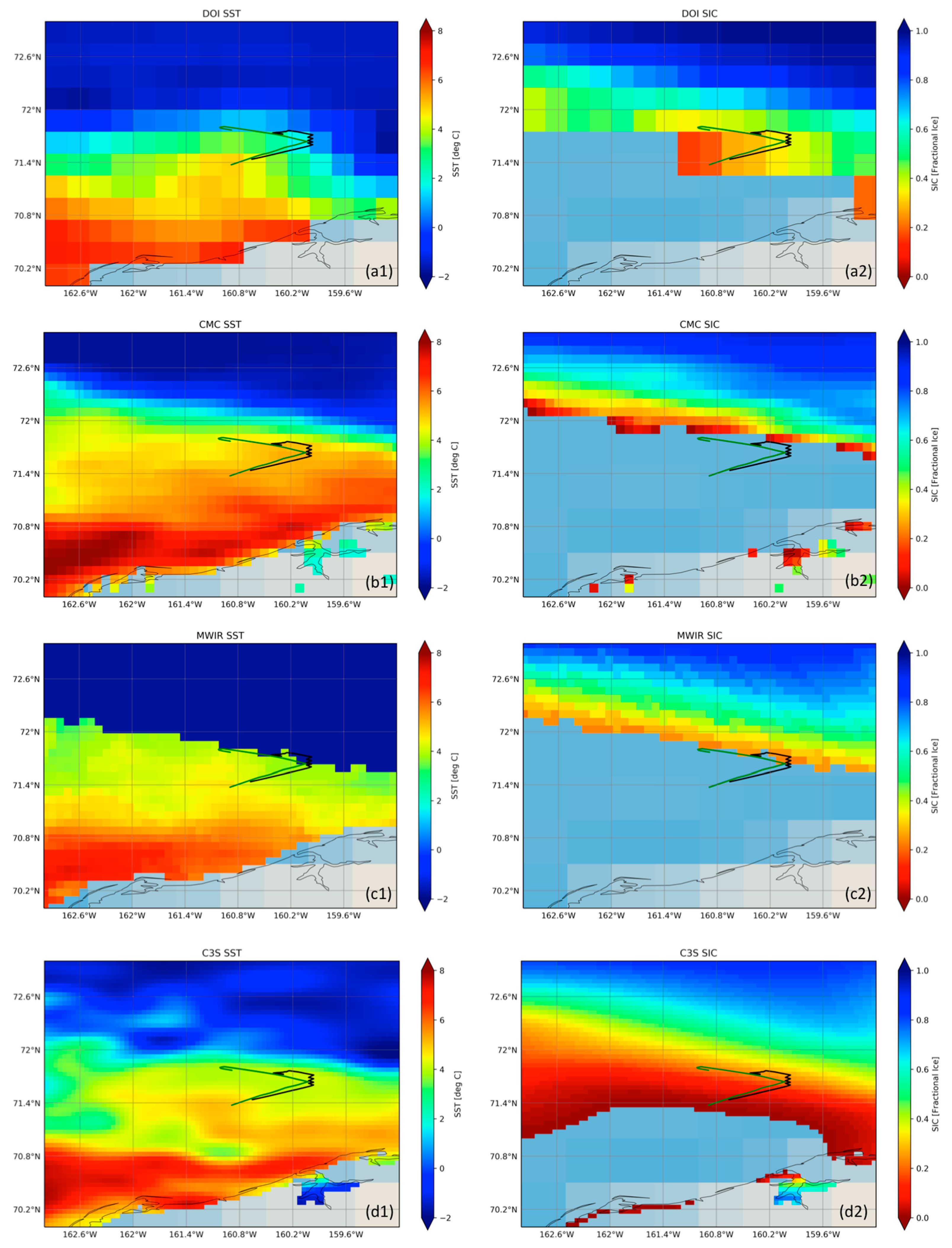
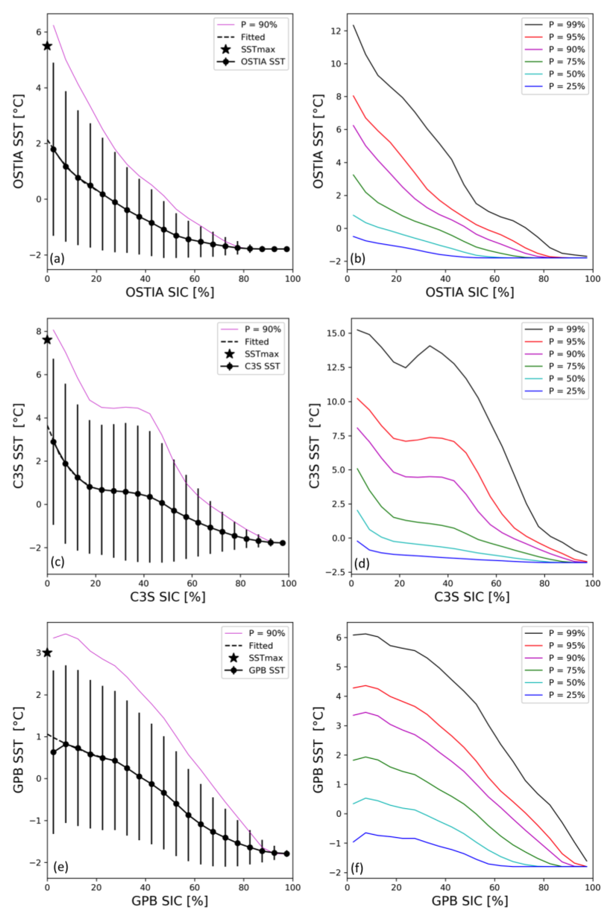
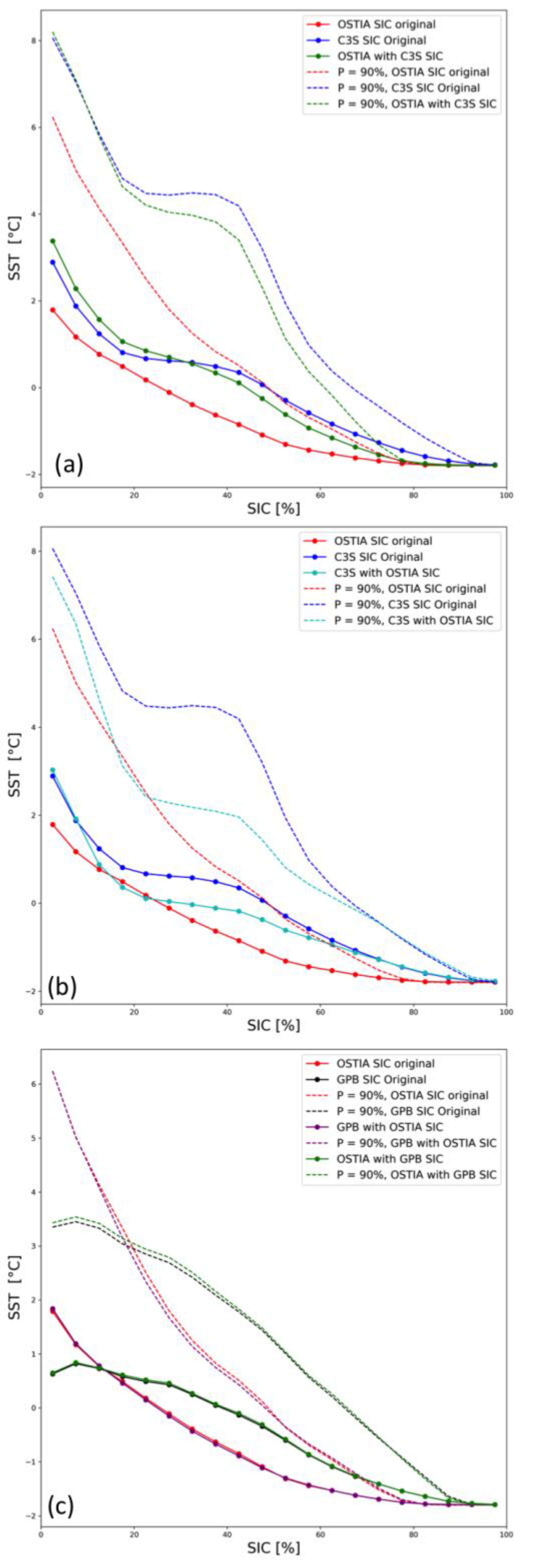
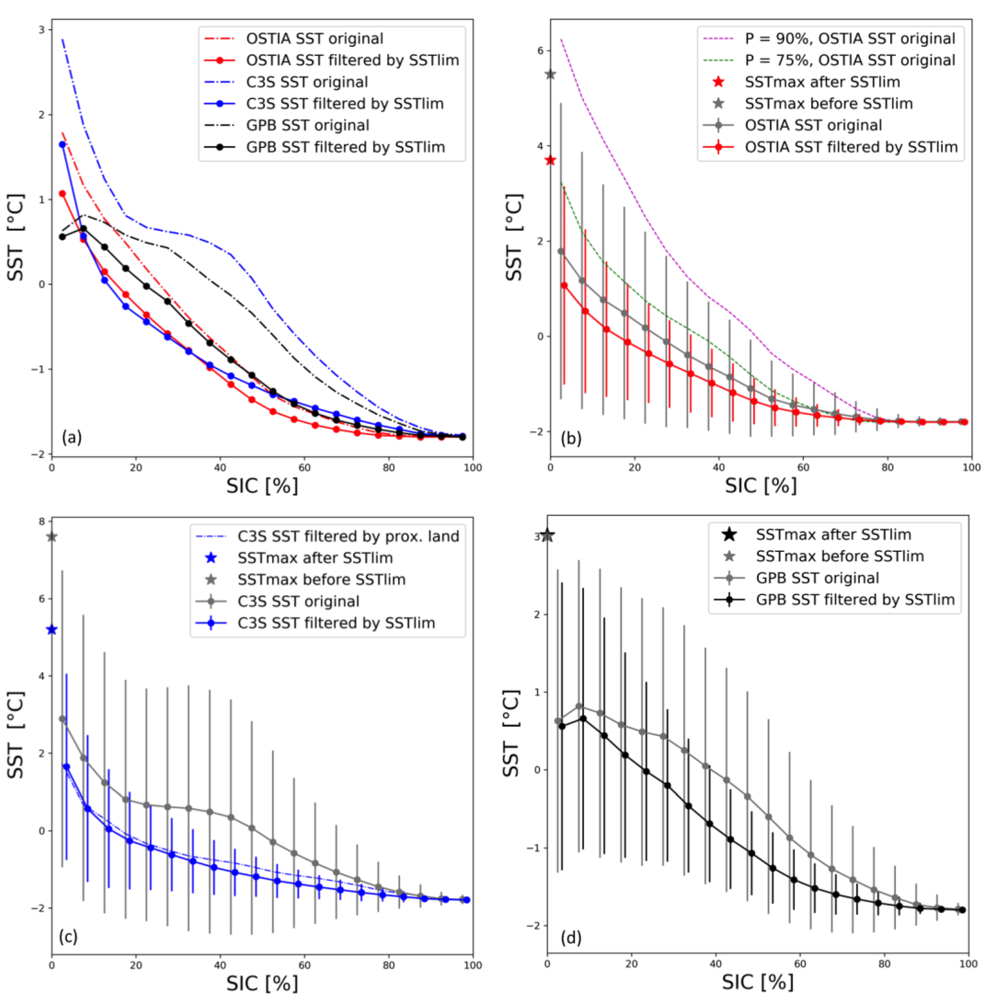
• The OSTIA SST vs. SIC interdependence appears to be exponential in nature with maximum SST of 6 °C for mixed pixels with very low ice concentrations (the maximum SST corresponds to a spatial average). We took the exponential shape of the OSTIA SST/SIC interdependence to be the model for mixed water/ice pixels, a fact later confirmed via numerical simulations;
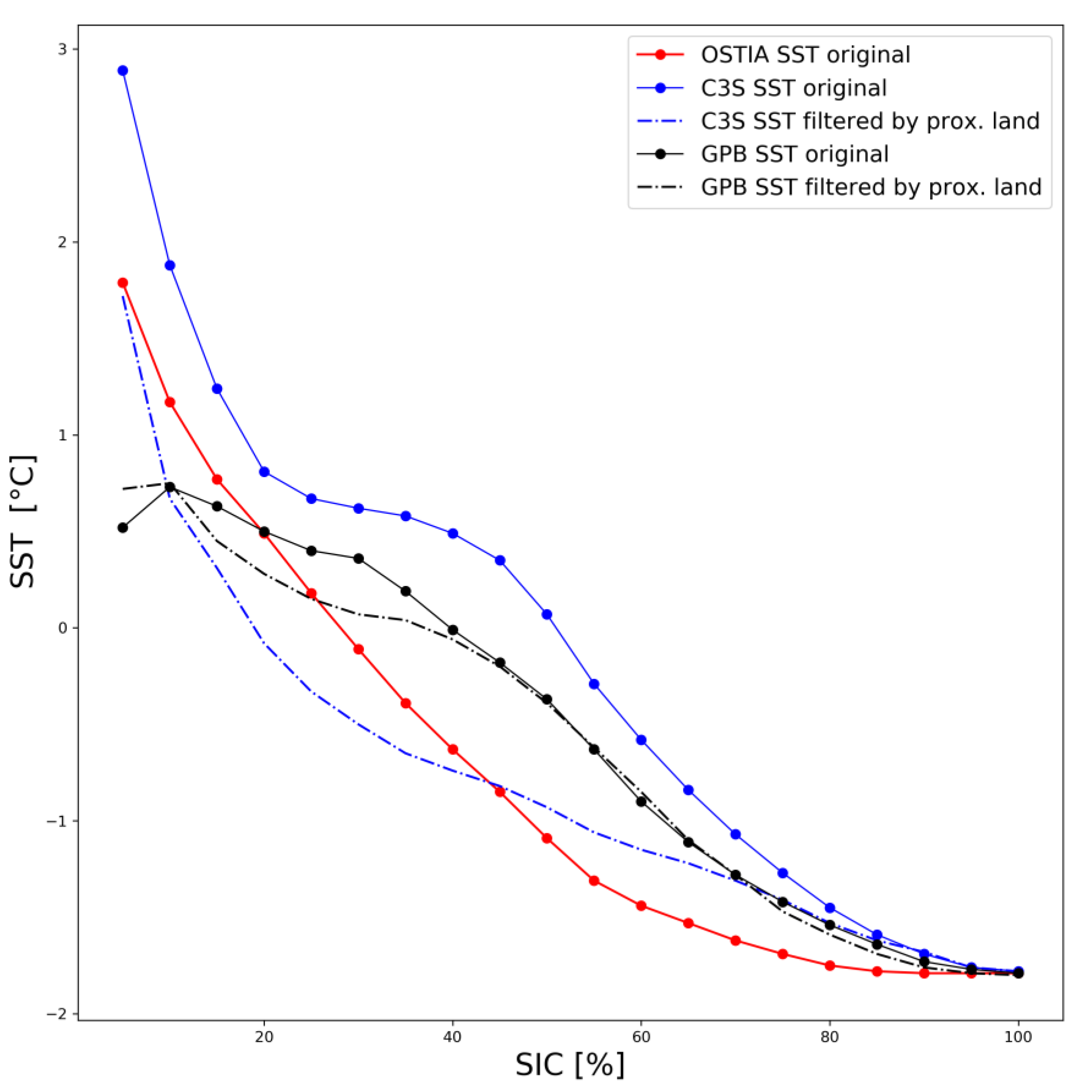
• The C3S SSTs also appear to be exponential, with an SST_max of 9 °C. The unfiltered SSTs appear to have a bump for 40–70%-SIC. This bump is artificially introduced into the OSTIA SST/SIC interdependence when the curve is reevaluated after switching the OSTIA SIC product with the C3S SIC product. When the C3S SIC is substituted by the OSTIA SIC, the bump is significantly reduced from the C3S SST/SIC curve, but not entirely eliminated, suggesting that the source of the errors introducing the bump affects both the C3S SST and corresponding SIC, but it affects the SSTs to a lesser degree. Further filtering of the C3S SSTs based on proximity to land suggests that the bump in C3S SST = f (SIC) is reduced by applying a more stringent filter for land contamination; and
• The GPB SST/SIC curve is significantly below the other two with a maximum SST of 3 °C for SIC ≈ 0%. This appears to be the result of the very restrictive open-water filter used by NCEP that eliminates all SIC retrievals with SST ≥ 2.15 °C. Furthermore, the curve has a different shape than the other two. The proximity-to-land filter has a minor impact on the shape of the SST/SIC distribution for the GPB product, most likely because the NCEP ice product only retrieves concentrations that are more than 100 km from land. The SIC used in this product combination, however, appears to be affected by grid projection errors.

The shape of the SST/SIC curve, hence, appears sensitive enough to the presence of erroneous retrievals in either of the products. An accurate knowledge of the SST/SIC interdependence offers an alternative way to eliminate spurious retrievals that do not follow the laws of thermodynamics governing the interdependence between the two variables. The parametric exponential fit for the SST vs. SIC interdependence was found via a simulation study in a mixed water/ice square pixel of 5 km-length (the same spatial resolution of the products considered here) and proposed as a new correction scheme in which (SST, SIC) pairings with SST > SST_lim are eliminated from the working data set. The rationale is that (SST, SIC) pairs that do not conform with the SST marginal distribution for a given SIC are subject to anomalous values for at least one of the quantities. It is important to emphasize that the filter adjusts for the effect of the simultaneous variations between SST and SIC, even though the erroneous estimate could be in the SICs but not in the SSTs, or vice versa. It could also be in both variables as suggested by the bump in the C3S SST/SIC interdependence, but the fact that the source of the error affected the SICs more than the SSTs, suggests that many of the warm SSTs that constituted the bump were correct but corresponded to mixed pixels with less ice than what was indicated by the SIC product. This implies that the SST_lim filter can be useful for quality control to remove biases on SIC inputs before the SST assimilation, or it could be used as an a posteriori filter to remove residual SIC inconsistencies. The proposed filter has the potential to reduce uncertainties as observed in the adjusted SST/SIC curves (both in mean and SD), after the SST_lim filter was applied to each of the products’ 2019 data. For OSTIA, it removed 15% of the top outliers consistently across SIC bins and the SD decreased from 0.68 °C to 0.52 °C; for C3S, the filter removed the bump in the midrange SICs and the SD decreased from 1.34 °C to 0.61 °C; for GPB, it changed the concavity of the SST/SIC curve in a manner consistent with the other two, and the SD decreased from 0.71 °C to 0.58 °C. The reduced SST variability in the filtered data is in agreement with the SST global accuracy requirements. New SST_max for SIC ≈ 0% after the SST_lim filter was applied were 4 °C, 5 °C, and 3 °C for OSTIA, C3S, and GPB, respectively. These values are below the theoretical limit of 7.4 °C obtained from the parametric exponential equation. The new SST_lim filter has the potential for homogenizing the SST = f (SIC) distributions relative to the OSTIA reference.

Sensitivity analyses for the simulation parameters (SST_max, SST_min, and the SST gradient) support an SST ceiling for a pixel containing any ice of 3 °C, a value commonly cited in reference to the SST_critic of SIC analyses for average characteristics at spatial resolutions of 15–25 km. For finer resolutions and more localized variability, the maximum thermal capacity of a pixel partially covered by ice appears to be above the standard SST_critic. The simulation results also suggested SST gradients larger than the values reported in the literature with the current state-of-the-art L4 SST products and their attainable feature resolution. Those gradients, however, were in excellent agreement with SST gradients measured from the Saildrones. According to the sensitivity tests, the SST_max increases as the strength of the gradient increases, but finer spatial resolutions demand stronger gradients near the ice. For spatial resolution grids of 5 km and gradients consistent with the Saildrone measurements, an SST_max of 4 °C would be required, which is consistent with the value obtained from the OSTIA SST/SIC curve after the SST_lim filter was applied. The simulation study does not consider thermal fronts that cover a portion of the pixel other than a corner of the domain. This is potentially an issue for coarser resolution pixels, as SST fronts tend to be long and narrow spatial features, but by locating the ice at one corner of the pixel, it gives the maximum gradient attainable within the pixel.

Application of the new SST_lim filter to the Saildrone-SST matchups from the three L4 SST products showed skill at reducing the robust RMS. The most effective correction schemes are those that yield the lowest RRMS. The SST/SIC interdependence needs further verification with an independent, larger observational data set such as buoys. Since the SST_lim filter is grid-size dependent, application to other L4 SST products with different resolution would need to be reevaluated.

References

1. Castro, S. Sea Surface Temperature Metrics for Evaluating OSI SAF Sea Ice Concentration Products, OSI SAF Visiting Scientist Program Report, OSI_AS19_04. October 2019, p. 67. Available online: https://osi-saf.eumetsat.int/sites/osi-saf.eumetsat.int/files/inline-files/OSI_VS19_04_DMI_VS_final_report_castro.pdf (accessed on 27 February 2023).
2. Hurrell, J.W.; Hack, J.J.; Shea, D.; Caron, J.M.; Rosinski, J. A New Sea surface Temperature and Sea Ice Boundary Dataset for the community Atmosphere Model. J. Clim. 2008, 21, 5145–5153. [Google Scholar] [CrossRef]
3. Ivanova, N.; Pedersen, L.T.; Tonboe, R.T.; Kern, S.; Heygster, G.; Lavergne, T.; Sørensen, A.; Saldo, R.; Dybkjær, G.; Brucker, L.; et al. Inter-comparison and evaluation of sea ice algorithms: Towards further identification of challenges and optimal approach using passive microwave observations. Cryosphere 2015, 9, 1797–1817. [Google Scholar] [CrossRef] [Green Version]
4. Lavergne, T.; Sørensen, A.M.; Kern, S.; Tonboe, R.; Notz, D.; Aaboe, S.; Bell, L.; Dybkjær, G.; Eastwood, S.; Gabarro, C.; et al. Version 2 of the EUMETSAT OSI SAF and ESA CCI sea-ice concentration climate data records. Cryosphere 2019, 13, 49–78. [Google Scholar] [CrossRef] [Green Version]
5. Andersen, S.; Tonboe, R.; Kern, S.; Schyberg, H. Improved retrieval of sea ice total concentration from spaceborne passive microwave observations using Numerical Weather Prediction model fields: An intercomparison of nine algorithms. Remote Sens. Environ. 2006, 104, 374–392. [Google Scholar] [CrossRef]
6. Hwang, B.J.; Barber, D.J. Pixel-scale evaluation of SSM/I sea-ice algorithms in the marginal ice zone during early fall freeze-up. Hydrol. Process. 2006, 20, 1909–1927. [Google Scholar] [CrossRef]
7. Tonboe, R.T.; Nandad, V.; Mäkynen, M.; Pederson, L.-T.; Kern, S.; Lavergne, T.; Øelund, J.; Dybkjær, G.; Saldo, R.; Huntemann, M. Simulated Geophysical Noise in Sea Ice Concentration Eestimates of Open Water and Snow-covered Sea Ice. IEEE J. Sel. Top. Appl. Earth Obs. Remote Sens. 2021, 15, 1309–1326. [Google Scholar] [CrossRef]
8. Gloersen, P.; Cavalieri, D.J. Reduction of weather effects in the calculation of sea ice concentration from microwave radiances. J. Geophys. Res. 1986, 91, 3913–3919. [Google Scholar] [CrossRef]
9. Cavalieri, D.J.; Crawford, J.P.; Drinkwater, M.R.; Emery, W.J.; Eppler, D.T.; Farmer, L.D.; Fowler, C.W.; Goodberlet, M.; Jentz, R.R.; Milman, A.; et al. NASA Sea Ice Validation Program for the Defense Meteorological Satellite Program Special Sensor Microwave Imager: Final Report. NASA-TM-104559 1992. National Aeronautics and Space Administration, Goddard Space Flight Center, Greenbelt, MD, 1992. p. 126. Available online: https://ntrs.nasa.gov/api/citations/19920015007 (accessed on 24 February 2023).
10. Lavergne, T.; Tonboe, R.; Lavelle, J.; Eastwood, S. Algorithm Theoretical Basis Document for the OSI SAF Global Sea Ice Concentration Climate Data Record, OSI-450, OSI-430-b, Version 1.2, 14 March 2019, EUMETSAT Ocean and Sea Ice SAF High Latitude Processing Centre. 2019. Available online: https://osisaf-hl.met.no/sites/osisaf-hl/files/baseline_document/osisaf_cdop3_ss2_atbd_sea-ice-conc-climate-data-record_v1p2.pdf (accessed on 28 February 2023).
11. Maaß, N.; Kalescke, L. Improving passive microwave sea ice concentration algorithms for coastal areas: Applications to the Baltic Sea. Tellus A 2010, 62, 393–410. [Google Scholar] [CrossRef] [Green Version]
12. Parkinson, C.L.; Comiso, J.C.; Zwally, H.J.; Cavalieri, D.J.; Gloersen, P.; Campbell, W.J. Arctic Sea Ice, 1973–1976: Satellite Passive-Microwave Observations; NASA-SP-489 1987, National Aeronautics and Space Administration, Scientific and Technical Information Branch, Washington, DC. Available online: https://ntrs.nasa.gov/citations/19870015437 (accessed on 24 February 2023).
13. Markus, T.; Cavalieri, D.J. The AMSR-E NT2 sea ice concentration algorithm: Its basis and implementation. J. Remote Sens. Soc. Jpn. 2009, 29, 216–225. [Google Scholar] [CrossRef]
14. Meier, W.N.; Stroeve, J.; Fetterer, F.; Savoie, M.; Wilcox, H. Polar Stereographic Valid Ice Masks Derived from National Ice Center Monthly Sea Ice Climatologies, Version 1. User Guide. Boulder, CO, 2015, NASA National Snow and Ice Data Center Distributed Active Archive Center. Available online: https://doi.org/10.5067/M4PUJAQRI2DS (accessed on 24 February 2023).
15. Grumbine, R.W. A Posteriori Filtering of Sea Ice Concentration Analyses. NOAA/NWS/NCEP/EMC MMAB Tech. Note 282. 2009; p. 7. Available online: https://polar.ncep.noaa.gov/mmab/papers/tn282/posteriori.pdf (accessed on 27 February 2023).
16. Thiebaux, J.; Rogers, E.; Wang, W.; Katz, B. A New High-Resolution Blended Real-Time Global Sea Surface Temperature Analysis. Bull. Am. Meteor. Soc. 2003, 84, 645–656. [Google Scholar] [CrossRef] [Green Version]
17. Baordo, F.; Vargas, L.F.; Howe, E. OSI SAF Product User Manual for Global Sea Ice Concentration Level 2 and Level 3, OSI-410-a, OSI-401-d, OSI-408-a. Version 1, 1/11/2022. Available online: https://osisaf-hl.met.no/sites/osisaf-hl/files/user_manuals/osisaf_pum_ice-conc_l2-3_v1p0.pdf (accessed on 8 March 2023).
18. Nielsen-Englyst, P.; Høyer, J.L.; Kolbe, W.M.; Dybkjær, G.; Lavergne, T.; Tonboe, R.T.; Skarpalezoz, S.; Karagali, I. A combined sea and sea-ice surface temperature climate dataset of the Arctic, 1982–2021. Remote Sens. Environ. 2023, 284, 113331. [Google Scholar] [CrossRef]
19. Castro, S.L.; Wick, G.A.; Steele, M. Validation of satellite sea surface temperature analyses in the Beaufort Sea using UpTempO buoys. Remote Sens. Environ. 2016, 187, 458–475. [Google Scholar] [CrossRef]
20. Brasnett, B. The impact of satellite retrievals in a global sea-surface-temperature analysis. Q. R. Meteorol. Soc. 2008, 134, 1745–1760. [Google Scholar] [CrossRef]
21. Caya, A.; Buehner, M.; Carrieres, T. Analysis and Forecasting of Sea Ice Conditions with Three-Dimensional Variational Data Assimilation and a Coupled Ice-Ocean Model. J. Atmos. Oceanic Technol. 2010, 27, 353–369. [Google Scholar] [CrossRef]
22. GHRSST Science Team. The Recommended GHRSST Data Specification (GDS) 2.0, Document Revision 5; Available from the GHRSST International Project Office; 2012; p. 123. Available online: https://podaactools.jpl.nasa.gov/drive/files/OceanTemperature/ghrsst/docs/GDS20r5.pdf (accessed on 24 February 2023).
23. Wick, G.A.; Jackson, D.L.; Castro, S.L. Assessing the ability of satellites to resolve spatial sea surface temperature variability-The Northwest Tropical Atlantic ATOMIC Region. Remote Sens. Environ. 2023, 284, 113377. [Google Scholar] [CrossRef]
24. Vasquez-Cuervo, J.; Castro, S.L.; Steele, M.; Gentemann, C.; Gomez-Valdes, J.; Tang, W. Comparison of GHRSST SST Analysis in the Arctic Ocean and Alaskan Coastal Waters Using Saildrones. Remote Sens. 2022, 14, 692. [Google Scholar] [CrossRef]
25. Good, S.; Fiedler, E.; Mao, C.; Martin, M.J.; Maycock, A.; Reid, R.; Robert-Jones, J.; Searle, T.; Waters, J.; While, J.; et al. The Current Configuration of the OSTIA System for Operational Production of Foundation Sea Surface Temperature and Ice Concentration Analyses. Remote Sens. 2020, 12, 720. [Google Scholar] [CrossRef] [Green Version]
26. Donlon, C.J.; Martin, M.; Stark, J.; Roberts-Jones, J.; Fiedler, E.; Wimmer, W. The Operational Sea Surface Temperature and Sea Ice Analysis (OSTIA) system. Remote Sens. Environ. 2012, 116, 140–158. [Google Scholar] [CrossRef]
27. Mogensen, K.S.; Alonso-Balmaseda, M.; Weaver, A. The NEMOVAR Ocean Data Assimilation System as Implemented in the ECMWF Ocean Analysis for System 4. ECMWF Tech. Memorandum 668, 2012, p. 59. ECMWF, Reading, UK. Available online: https://www.ecmwf.int/en/elibrary/75708-nemovar-ocean-data-assimilation-system-implemented-ecmwf-ocean-analysis-system-4 (accessed on 28 February 2023).
28. Reynolds, R.W.; Smith, T.M.; Liu, C.; Chelton, D.B.; Casey, K.S.; Schlax, M.G. Daily High-Resolution-Blended Analyses for Sea Surface Temperature. J. Clim. 2007, 20, 5473–5496. [Google Scholar] [CrossRef]
29. Tonboe, R.; Lavelle, J.; Pfiffer, R.-H.; Howe, E. Product User Manual for OSI SAF Global Sea Ice Concentration, Product OSI-401-b, Version 1.6. Tech. Rep. SAF/OSI/COP3/DMI_MET/TEC/MA/204. Danish Meteorological Institute. 2017, p. 25. Available online: https://osisaf-hl.met.no/sites/osisaf-hl/files/user_manuals/osisaf_cdop3_ss2_pum_ice-conc_v1p6.pdf (accessed on 28 February 2023).
30. Robert-Jones, J.; Bovis, K.; Matthew, M.J.; McLaren, A. Estimating background error covariance parameters and assessing their impact in the OSTIA system. Remote Sens. Environ. 2016, 176, 117–138. [Google Scholar] [CrossRef]
31. Fiedler, E.K.; Mao, C.; Good, S.A.; Waters, J.; Martin, M.J. Improvements to feature resolution in the OSTIA sea surface temperature analysis using the NEMOVAR assimilation scheme. Q. J. R. Meteorol. Soc. 2019, 145, 3609–3625. [Google Scholar] [CrossRef]
32. Mirouze, I.; Blockley, E.W.; Lea, D.J.; Martin, M.J.; Bell, M.J. A multiple length scale correlation operator for ocean data assimilation. Tellus A Dyn. Meteorol. Oceanogr. 2016, 68, 29744. [Google Scholar] [CrossRef] [Green Version]
33. Merchant, C.J.; Embury, O.; Roberts-Jones, J.; Fiedler, E.; Bulgin, C.E.; Corlett, G.K.; Good, S.; McLaren, A.; Rayner, N.; Morak-Bozzo, S.; et al. Sea surface temperature datasets for climate applications from Phase 1 of the European Space Agency Climate Change Initiative (SST CCI). Geosci. Data J. 2014, 1, 179–191. [Google Scholar] [CrossRef] [Green Version]
34. Merchant, C.J.; Embury, O.; Bulgin, C.E.; Block, T.; Corlett, G.K.; Fiedler, E.; Good, S.A.; Mittaz, J.; Rayner, N.A.; Berry, D.; et al. Satellite-based time-series of sea-surface temperature since 1981 for climate applications. Sci. Data 2019, 6, 223. [Google Scholar] [CrossRef] [Green Version]
35. Merchant, C.J.; The CCI SST Team. SST-CCI-Phase-II, SST CCI Algorithm Theoretical Basis Document (v2 Reprocessing). SST_CCI-ATBD-UOR-203, Issue 3. 6 May 2019. Available online: https://climate.esa.int/media/documents/SST_cci_ATBD_UOR_v3.pdf (accessed on 28 February 2023).
36. Lu, J.; Heygster, G.; Spreen, G. Atmospheric correction of sea ice concentration retrievals for 89 GHz AMSR-E observations. IEEE J. Sel. Top. Appl. Earth Obs. Remote Sens. 2018, 11, 5. [Google Scholar] [CrossRef]
37. Maturi, E.; Harris, A.; Mittaz, J.; Sapper, J.; Wick, G.; Zhu, X.; Dash, P.; Koner, P. A New High-Resolution Sea Surface Temperature Blended Analysis. Bull. Am. Meteor. Soc. 2017, 98, 1015–1026. [Google Scholar] [CrossRef]
38. Liu, G.; Heron, S.F.; Eakin, C.M.; Muller-Karger, F.E.; Vega-Rodriguez, M.; Guild, L.S.; De La Cour, J.L.; Geiger, E.F.; Skirving, W.J.; Burgess, T.F.R.; et al. Reef-Scale Thermal Stress Monitoring of Coral Ecosystems: New 5-km Global Products from NOAA Coral Reef Watch. Remote Sens. 2014, 6, 11579–11606. [Google Scholar] [CrossRef] [Green Version]
39. Grumbine, R.W. Automated Sea Ice Concentration Analysis History at NCEP: 1996–2012. NOAA/NWS/NCEP/EMC MMAB Tech. Note 321. 2014; p. 39. Available online: https://polar.ncep.noaa.gov/mmab/papers/tn321/MMAB_321.pdf (accessed on 27 February 2023).
40. Gemmill, W.; Katz, B.; Li, X. Daily Real-Time, Global Sea Surface Temperature High-Resolution Analysis: RTG_SST_HR. NOAA/NWS/NCEP/EMC/MMAB Tech. Note 260. 2007; p. 22. Available online: http://polar.ncep.noaa.gov/mmab/papers/tn260/MMAB260.pdf (accessed on 27 February 2023).
41. Huang, B.; Liu, C.; Banzon, V.; Freeman, E.; Graham, G.; Hankins, B.; Smith, T.; Zhang, H.-M. Improvements of the Daily Optimum Interpolation Sea Surface Temperature (DOISST) Version 2.1. J. Clim. 2021, 34, 2923–2939. [Google Scholar] [CrossRef]
42. Banzon, V.; Smith, T.M.; Chin, T.M.; Liu, C.; Hankins, W. A long-term record of blended satellite and in situ sea-surface temperature for climate monitoring, modeling, and environmental studies. Earth Syst. Sci. Data 2016, 8, 165–176. [Google Scholar] [CrossRef] [Green Version]
43. Banzon, V.; Smith, T.M.; Steele, M.; Huang, B.; Zhang, H.-M. Improved Estimation of Proxy Sea Surface Temperature in the Arctic. J. Atmos. Oceanic Technol. 2020, 37, 341–349. [Google Scholar] [CrossRef]
44. Brasnett, B.; Surcel-Colan, D. Assimilating Retrievals of Sea Surface Temperature from VIIRS and AMSR2. J. Atmos. Ocean. Technol. 2016, 33, 361–375. [Google Scholar] [CrossRef]
45. Rayner, N.A.; Parker, D.E.; Horton, E.B.; Folland, C.K.; Alexander, L.V.; Rowell, D.P.; Kent, E.C.; Kaplan, A. Global analyses of sea surface temperature, sea ice, and night marine air temperature since the late nineteenth century. J. Geophys. Res. 2003, 108, 4407. [Google Scholar] [CrossRef] [Green Version]
46. Buehner, M.; Caya, A.; Pogson, L.; Carrieres, T.; Pestieau, P. A New Environment Canada Regional Ice Analysis System. Atmos. Ocean 2013, 51, 18–34. [Google Scholar] [CrossRef]
47. Halliday, D.; Resnick, R. Fundamentals of Physics; Wiley: Hoboken, NJ, USA, 1974; p. 827. [Google Scholar]
48. Charron, M.; Polavarapu, S.; Buehner, M.; Vaillancourt, P.A.; Charette, C.; Roch, M.; Morneau, J.; Garand, L.; Aparicio, J.M.; MacPherson, S.; et al. The Stratospheric Extension of the Canadian Global Deterministic Medium-Range Weather Forecasting System and Its Impact on Tropospheric Forecasts. Mon. Weather Rev. 2012, 140, 1924–1944. [Google Scholar] [CrossRef]
49. Lavelle, J.; Tonboe, R.; Tian, T.; Pfeiffer, R.-H.; Howe, E. Product User Manual for the OSI SAF AMSR-2 Global Sea Ice Concentration, Product OSI-408, Version 1.1. Tech. Rep. SAF/OSI/COP2/DMI/TEC/265. The Danish Meteorological Institute. 2016, p. 28. Available online: https://osisaf-hl.met.no/sites/osisaf-hl/files/user_manuals/osisaf_cdop2_ss2_pum_amsr2-ice-conc_v1p1.pdf (accessed on 1 March 2023).
50. Gentemann, C.L.; Scott, J.P.; Mazzini, P.L.F.; Pianca, C.; Akella, S.; Minnett, P.J.; Cornillon, P.; Fox-Kemper, B.; Cetinic, I.; Chin, T.M.; et al. Saildrone: Adaptively Sampling the Marine Environment. Bull. Am. Meteorol. Soc. 2020, 101, 744–762. [Google Scholar] [CrossRef] [Green Version]
51. Chiodi, A.M.; Zhang, C.; Cokelet, E.D.; Yang, Q.; Mordy, C.W.; Gentemann, G.; Cross, J.N.; Lawrence-Slavas, N.; Meining, C.; Steele, M.; et al. Exploring the Pacific Arctic Seasonal Ice Zone with Saildrone USVs. Front. Mar. Sci. 2021, 8, 640690. [Google Scholar] [CrossRef]
52. May, D.A.; Parmeter, M.M.; Olszewski, D.S.; McKenzie, B.D. Operational Processing of Satellite Sea Surface Temperature Retrievals at the Naval Oceanographic Office. Bull. Am. Meteor. Soc. 1998, 79, 397–407. [Google Scholar] [CrossRef]
53. Richter-Menge, J.; Perovich, D.K.; Pegau, W.S. Summer ice dynamics during SHEBA and its effect on the ocean heat content. Ann. Glaciol. 2001, 33, 201–206. [Google Scholar] [CrossRef] [Green Version]
54. Perovich, D.K.; Maykut, G.A. Solar heating of a stratified ocean in the presence of a static ice cover. J. Geophys. Res. 1990, 95, 18233–18245. [Google Scholar] [CrossRef]
55. Perovich, D.K.; Tucker, W.B., III; Ligett, K.A. Aerial observations of the evolution of ice surface conditions during summer. J. Geophys. Res. 2002, 107, 8048. [Google Scholar] [CrossRef]
Figure 1. Saildrone tracks for the 2019 MISST Arctic Campaign, color-coded by the Saildrone’s SBE56 temperatures in degrees Celsius: (a) SD1036 and (b) SD1037.
Remotesensing 15 02908 g001
Figure 2. Time series of SSTs from the Saildrone’s SBE56 thermistor (black) and the L4 SST analyses collocated with the Saildrones (red: SD1036, blue: SD1037) for: (a1,a2): DOISST; (b1,b2): CMC; (c1,c2): MWIR; (d1,d2): C3S; (e1,e2): OSTIA; and (f1,f2): GPB.
Remotesensing 15 02908 g002
Figure 3. Ice along the Saildrone paths estimated from the matchups with the L4 SIC product distributed with the L4 SSTs. (a) (SD1036) and (b) (SD1037) show all of the SIC/Saildrone matchups corresponding to the entire duration of the 2019 Saildrone campaign, with the X-axis displaying the corresponding day-of-year (DOY). (c) (SD1036) and (d) (SD1037) zoom in the SIC matchups for DOY 167–177.
Remotesensing 15 02908 g003
Figure 4. Maps of SST (left column) and corresponding SIC (right column) centered around the Saildrone tracks (SD1036: black; SD1037: green) for 22 June 2019 (DOY 173): (a1,a2): DOISST; (b1,b2): CMC; (c1,c2): MWIR; (d1,d2): C3S; (e1,e2): OSTIA; and (f1,f2): GPB.
Remotesensing 15 02908 g004aRemotesensing 15 02908 g004b
Figure 5. Time series of Saildrone temperatures (black, (a1): SD1036; (b1): SD1037) and L4 SST products for DOY 167–177, and corresponding residual SST differences with respect to the Saildrone ((a2): L4 SST—SD1036 SST; (b2): L4 SST—SD1037 SST).
Remotesensing 15 02908 g005
Figure 6. Map of OSTIA SST around the Saildrone paths (SD1036: black; SD1037: red) for 19 June 2019 (DOY 170). Saildrone SD1037 cuts across the cold SST feature centered around (71.1N,162.3W), which is reflected in the negative dip in SBE56 temperatures for DOY 168–172 shown in Figure 5b2. Only the OSTIA product resolved this feature, as demonstrated by the good agreement between SD1037 (black) and OSTIA (blue) in Figure 5a2,b2.
Remotesensing 15 02908 g006
Figure 7. Two-dimensional histograms for the 2019 Arctic summer (May–September) L4 SSTs, and corresponding SIC data for (a) OSTIA, (b) C3S, and (c) GPB. Blue colors indicate a low density of counts and red colors indicate a high-density of counts.
Remotesensing 15 02908 g007
Figure 8. Error bar plots (left column) and percentile graphs (right column) showing the variability of the SST = f (SIC) for (a,b): OSTIA, (c,d): C3S, and (e,f): GPB. The error bar plots are given in 5%-ice concentration bins. The cumulative frequency curves correspond to the 25th, 50th, 75th, 90th, 95th, and 99th percentiles. The pink curve shown with the error bar plots is the same 90th percentile curve shown on the right for each of the L4 SST analysis.
Remotesensing 15 02908 g008
Figure 9. Mean SST/SIC interdependence for OSTIA (red), C3S (dark blue) and GPB (black) SST analyses based on the original L4 SIC analysis (same as Figure 8), and after exchanging the L4 SST’s associated SIC product for the OSTIA SIC: (a) OSTIA SST vs. C3S SIC (green), (b) C3S SST vs. OSTIA SIC (light blue), (c) OSTIA SST vs. GPB SIC (magenta) and GPB SST vs. OSTIA SIC (purple). The corresponding 90th percentile curves are also included.
Remotesensing 15 02908 g009
Figure 10. Original mean SST/SIC interdependence for C3S (dark blue) and GPB (black) SSTs (continuous curves, same as Figure 8), and after applying a proximity-to-land filter that eliminates (SST, SIC) pairs that are within 50 km from land (dash-dot curves). The original OSTIA mean SST/SIC interdependence in red is included for reference.
Remotesensing 15 02908 g010
Figure 11. The 2017 buoy SST-C3S SIC interdependence is in black for the 2017 Arctic summer C3S-GTS buoy matchups above 50N. In blue is the corresponding mean C3S SST/SIC interdependence at the buoy locations. While the C3S curve relaxes towards the freezing temperature of sea water, the buoy curve relaxes towards the triple point temperature of water.
Remotesensing 15 02908 g011
Figure 12. Illustration of the simulation realization (a) for a 5 km × 5 km spatial domain with 10%-ice cover and a minimum SST of 0 °C at the ice edge. At (b), the simulated SST values for 5%-SIC increments from 5% to 100% and the resulting parametric equation (SSTlim) describing the exponential function that best fits the simulation results.
Remotesensing 15 02908 g012
Figure 13. Evaluation of the application of the SSTlim equation as a post-processing filter to remove SIC inconsistencies/SST outliers in L4 SST and SIC analyses: (a) mean SST/SIC interdependence before (continuous curves; same as Figure 8) and after the application of the SSTlim filter (dash-dot curves) for the OSTIA (red), C3S (blue), and GPB (black) SST analyses. Error bar plots before (grey) and after the application of the SSTlim filter for (b) OSTIA (red), (c) C3S (blue), and (d) GPB (black). The stars (y-axis) for each of the L4 SST analysis indicate the SSTmax before (grey) and after (color) the filter. Included in Figure 13b are the 90th (magenta) and 75th (green) percentile graphs of the original data (before the SSTlim filter) showing how the proposed filter eliminated about 15% of the top OSTIA SST outliers in each of the SIC bins.
Remotesensing 15 02908 g013
Figure 14. SST = f (SIC) quantile–quantile plots for C3S against OSTIA (a) before and (c) after the application of the SSTlim filter, and for GPB against OSTIA (b) before and (d) after the application of the SSTlim filter. The Q–Q curves are for the 25th, 50th, 75th, 90th, 95th, and 99th percentiles. The 1:1 line (black dash) is given for reference purposes as samples with the same distribution will have Q–Q points aligned with the x-y line.
Remotesensing 15 02908 g014aRemotesensing 15 02908 g014b