1. Introduction
The mean sea surface (MSS) is an important field in physical oceanography, geophysics, and geodesy. In principle, it corresponds to the time-averaged height of the ocean surface. In practice, the goal is to achieve a complete separation of the ocean content into two distinct components, a variable part and a static part, over an arbitrary reference period. The first challenge consists in removing the variable part without deteriorating the topography of the geophysical structures, especially at the shortest wavelengths.
Until recently, MSS was restricted to ice-free ocean areas. For some years, dedicated processing to retrieve the sea level from fractures in ice, the leads, were developed, and MSS covering the global ice-covered Arctic region emerged [
1]. This includes the DTU15 MSS [
2] solution, which was used to produce Arctic-Sea-level maps covering the Arctic region up to 88°N [
3,
4]. In this paper, sea-level measurements within the ice-covered region were used to create a satellite-based MSS up to 88°N.
These different goals were reached by combining data from exact-repeat missions (ERMs) and very-high-resolution observations of non-repetitive altimetric missions. However, the use of geodetic and drifting data requires special attention due to the difficulty in obtaining direct and accurate access to the interannually and seasonally variable parts of the oceanic signal [
5].
In this paper, we present a brief overview of the data used, as well as some reminders about the treatments and mapping methods implemented, which have already been widely discussed in previous publications [
5,
6,
7,
8].
Our main purpose is to discuss in detail the latest upgrades of the methodology and processing. First, the use of full-rate altimetry data (20 Hz, 40 Hz) to improve the mapping of geophysical structures smaller 30 km is explained. The second improvement is the oceanic-variability processing, especially for wavelengths lower than 100 km, which is not fully resolved by DUACS MSLA [
9]. A final section is devoted to the analysis of the improvements of this new 2022 MSS compared to the previous version, the CNES_CLS 2015 MSS.
2. Altimeter-Data Processing
2.1. Altimeter Data for MSS Computation
2.1.1. Ocean Data
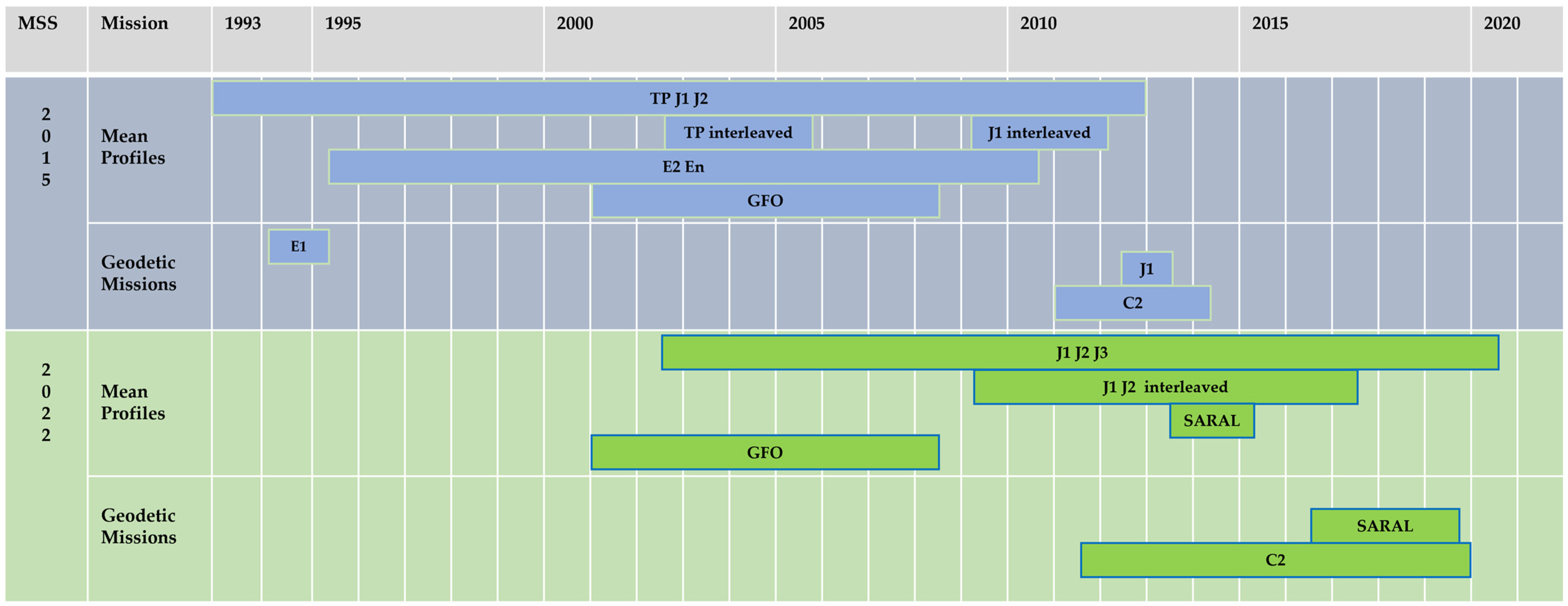
While the CNES_CLS 2015 MSS was computed using 1-Hz altimeter measurements, the CNES_CLS 2022 MSS is the result of the combination of mean profiles (MP) calculated from ERM that are still processed at 1 Hz and high-resolution data from the SARAL/Altika (SARAL) and CryoSat-2 (C2) geodetic (or drifting) missions, sampled at 40 Hz and 20 Hz, respectively.
An overview of the satellite missions considered and the periods available on the database that were used is presented in
Figure 1 (details of cycles used are presented in
Appendix A,
Table A1).
All these measurements were processed using altimeter standards and corrections corresponding to the DT-2021 version described in [
10]. The MSLA DT-2018 version [
11] was used to correct the SSH from the oceanic variability over the defined reference period [1993, 2012] for all the altimetric missions (see [
5] for details).
2.1.2. Arctic Data
In the polar regions, satellite sea-level observations are limited by sea ice. However, thanks to dedicated processing, sea levels can be estimated within fractures in ice (leads). The sea levels within the leads from three altimeters were ingested in the new CNES_CLS_2022 MSS to cover the Arctic region up to 88°N. The processing is explained in detail by Prandi et al. [
3]. Firstly, the echoes from the altimeters over the ice-covered region were classified to identify peaky waveforms corresponding to lead echoes, and then instrumental and geophysical corrections were applied, and editing processing was performed to remove outliers. An additional cross-calibration through optimal interpolation was performed to reduce the long-wavelength geographically correlated errors between the three altimetric missions (CryoSat-2, SARAL/AltiKa, and Sentinel-3A).
Table A2, presented in
Appendix A, summarizes the characteristics of the along-track input data. Note that the environmental and instrumental corrections applied to these data may be different from those used in the DT-2021 version (see
Table A2 in
Appendix A).
The reduction in ocean variability is a key process in the production of the MSS. For the Arctic region, sea-level-anomaly maps from June 2016 to June 2020, described by Prandi et al. [
3], were used to remove the ocean variability from the along-track leads of sea-surface height.
For some periods since 1993, no altimetry missions were conducted to sample the Arctic Ocean up to 88°N (especially before the start of Cryosat-2), so the reference period of the ice-covered region is more recent than that used for the open ocean. The leads MSS was calibrated on the open-ocean MSS using differences at the limit between the two surfaces. The aim was to homogenize the ice-covered reference period onto the open-ocean reference period, although, in the permanently ice-covered region, this period tended to be more recent.
2.1.3. The Correction of the Interannual and Seasonal Variability
The CNES_CLS 2022 MSS is based on the combination of altimeter data from different altimeter missions and covering different periods of time.
Figure 1 presents the satellite missions and time coverages that were used for the 2015 and 2022 MSSs. Except for the GeoSat Follow-On (GFO) MP, which covers the same period, the mean profiles used for the 2015 MSS cover a period from 1993 to 2013, while those for the 2022 MSS are from 2002 to 2020. The same holds for the geodetic missions, for which we have very distinct temporal coverage. For the 2015 MSS, we used ERS-1 between 1994 and 1995, and Jason-1 GM and CryoSat-2 between 2011 and 2014, whereas for the 2022 MSS, the geodetic data were from 2011 to 2019.
We also noticed that Topex/Poseidon (T/P), ERS-2 (E2), and EnviSat (En) were not reused because preliminary analyses showed that they provided a smoother sub-30-km-wavelength content than the most recent altimetric missions, which was due to a less performing retracking method. It should be noted that reprocessing is underway to improve this aspect, but this was not available when the mean profiles were prepared for this new MSS. Similarly, concerning the data from the geodetic missions, we preferred to focus on the use of SARAL and C2 observations sampled at higher frequencies than 1 Hz.
The first requirement was to homogenize all the datasets in terms of mean oceanic content, which should be as close as possible to the steady state of the ocean. Ideally, this should correspond to the sum of the geoid and the mean dynamic topography defined over a sufficient period to tend towards a constant value. This represents a major difficulty, as the data were acquired during various periods in the altimetry era. As already explained in previous papers ([
5,
8]), the correction of each observation based on a space–time interpolation of SLA is a clean way to ensure this homogeneity.
More specifically,
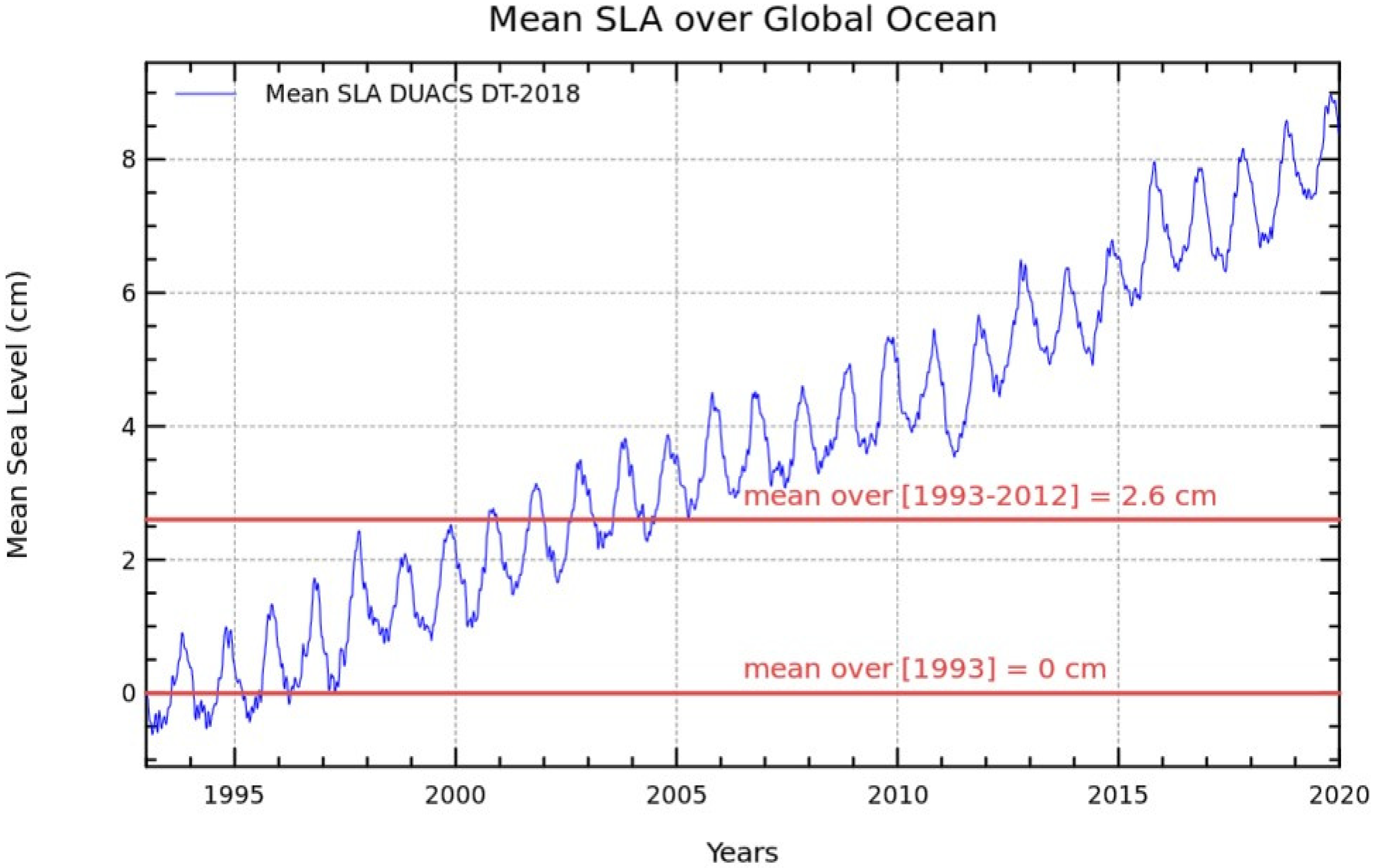
Figure 2 shows the evolution of the SLA over the years ranging from 1993 to 2020. As a convention, the average mean sea level for the year 1993 is artificially set to 0. This implies that any SSH corrected with this SLA is also corrected for sea-level rises (SLRs), but relative to the year 1993. We also note that the choice of the 20-year period for the mean content of the MSS implies an overall bias of 2.6 cm relative to 1993.
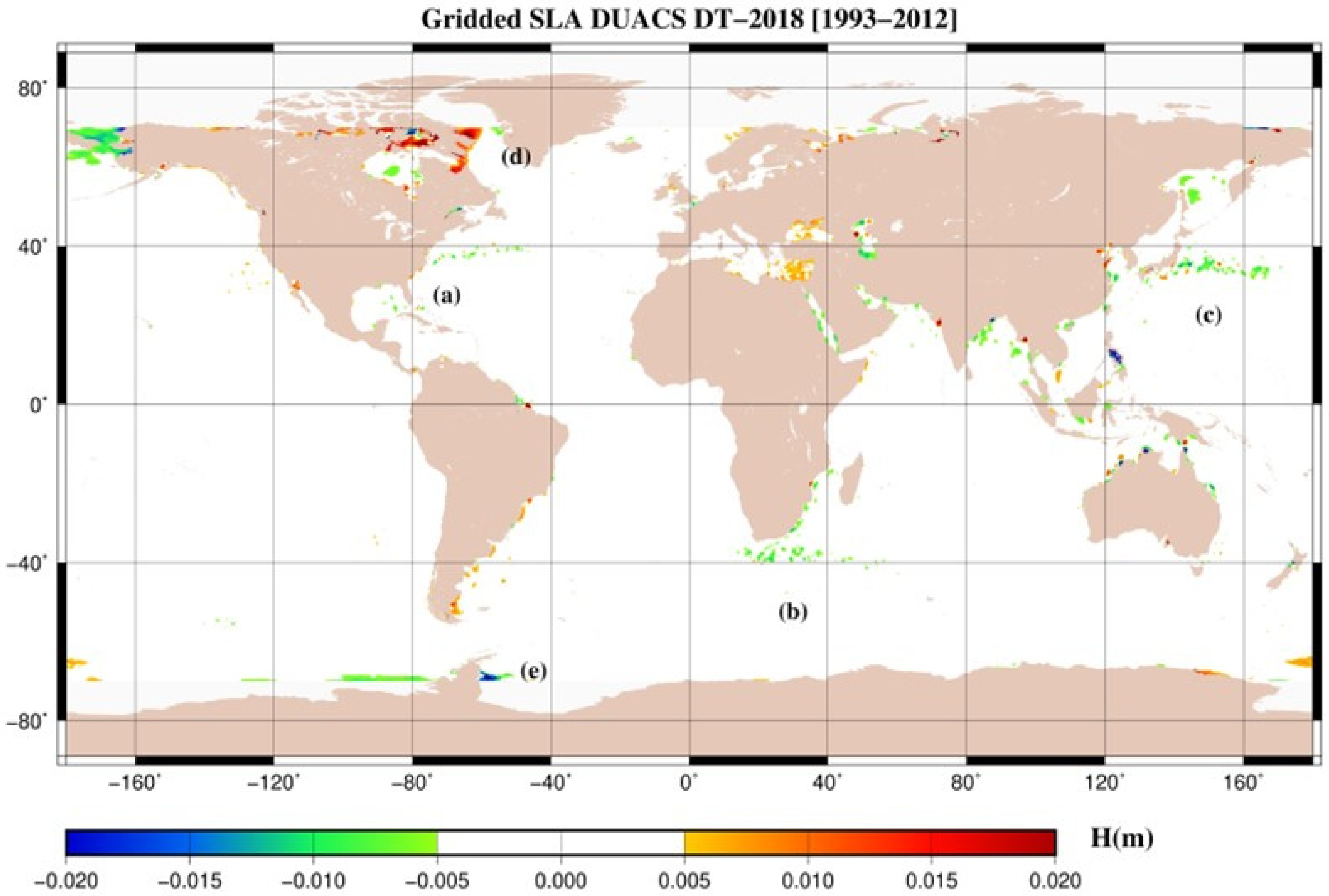
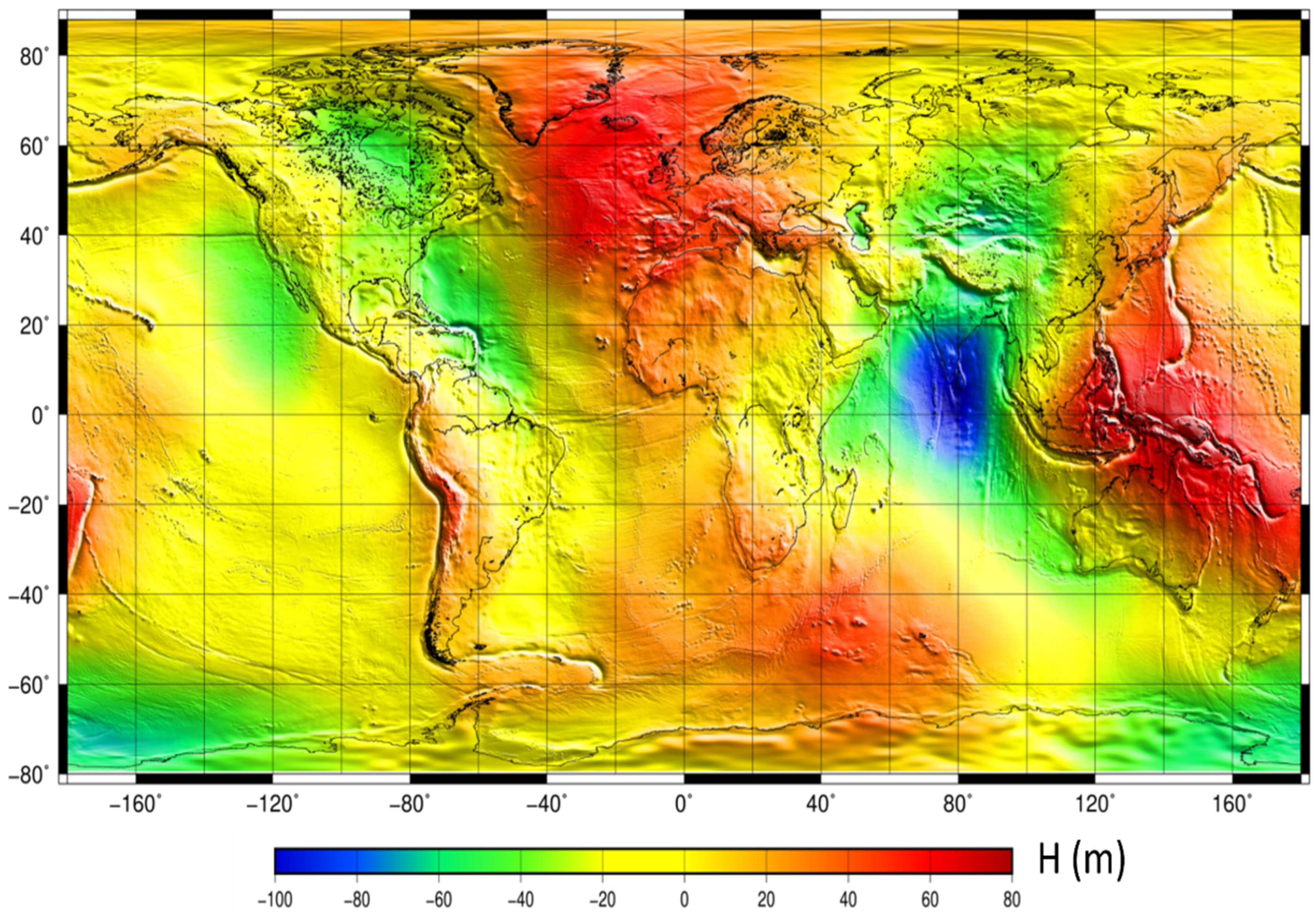
Furthermore, the map of the average of the DUACS MSLA gridded products calculated over this 20-year period (
Figure 3) was generally close to a constant value, which corresponded to this same bias of 2.6 cm, and the fact that no residual signals were present between ±5 mm showed that we were close to the ocean’s steady state.
However, two regional effects were observed. First, we noted a residual effect of the oceanic variability on areas with strong currents, such as the Gulf Stream (a), the Agulhas Current (b), and the Kuroshio (c). This was due to the difficulty in fully correcting the non-repetitive altimetric missions from the oceanic variability. Since, in contrast to the ERM, for which it is possible to compute averages over long periods, for non-repetitive missions, only DUACS MSLA maps are available, which do not contain the full amplitude of oceanic variability [
9]. This aspect is also one of major improvements made in the CNES_CLS 2022 solution, which is explained in more detail in
Section 3, especially concerning the omission error of the residual effect of the oceanic variability.
It should also be noted that the large discrepancies at high latitudes (d, e) were mainly due to the lack of continuous seasonal coverage from the repetitive missions, particularly those of Topex/Poseidon, Janson-1, Jason-2, and Jason-3 ERM, which are the most accurate but also the most continuous in time, and serve as a reference from 1993 to today. The decrease in observability for these regions resulted in a lower number of cycles with which to calculate the mean heights of the MP, which increased the standard deviation and, hence, the noise budget associated with each observation, which implicitly increased the formal error of the MSS (see Equation (3)).
2.2. Filtering of High-Resolution Data
Compared to the previous MSSs performed by CLS (2015, 2011, and 2001), which only used data sampled at 1 Hz (7 km) along-track, recent improvements in data processing allow us to access data at higher frequencies on C2 and SARAL with acceptable accuracy for the purpose of mapping the gravity field [
12], as well as MSS, in our case.
Thanks to the longevity of the C2 mission, the across-track density also reached a level that had never been achieved before. Considering that the optimal interpolation was based on selected observations in a subdomain, the combined use of C2 and SARAL sampled at 20 Hz and 40 Hz, respectively, allowed us to obtain, generally, more than 400 observations in influence bubbles with radii of about 10 km, whatever the area considered in the open ocean. In practice, this is statistically adequate for mapping topographic structures in the range of a few kilometers.
This approach is based on a covariance matrix that is normalized by the local variance of the signal, and a noise-to-signal ratio that is excessively high (a ratio greater than 70% is generally considered) can degrade the accuracy of the estimate. In addition to the spatial density of the observations, this parameter directly affects the quality of the restitution of topographic structures.
An example is given in
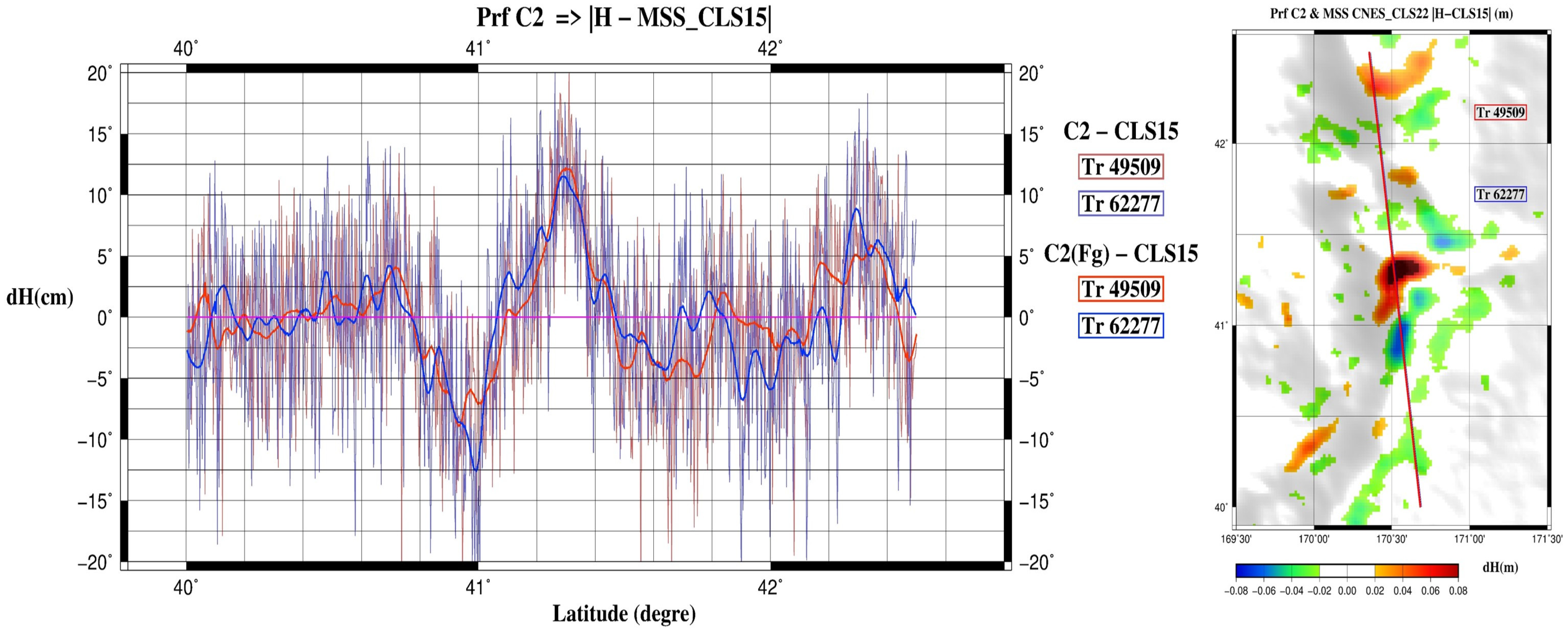
Figure 4. It shows a cross-sectional view of two C2 profiles that are only 700 m apart and that pass over a structure along the Emperor Seamount Chain, with amplitudes exceeding 8 cm relative to the CNES_CLS 2015 MSS.
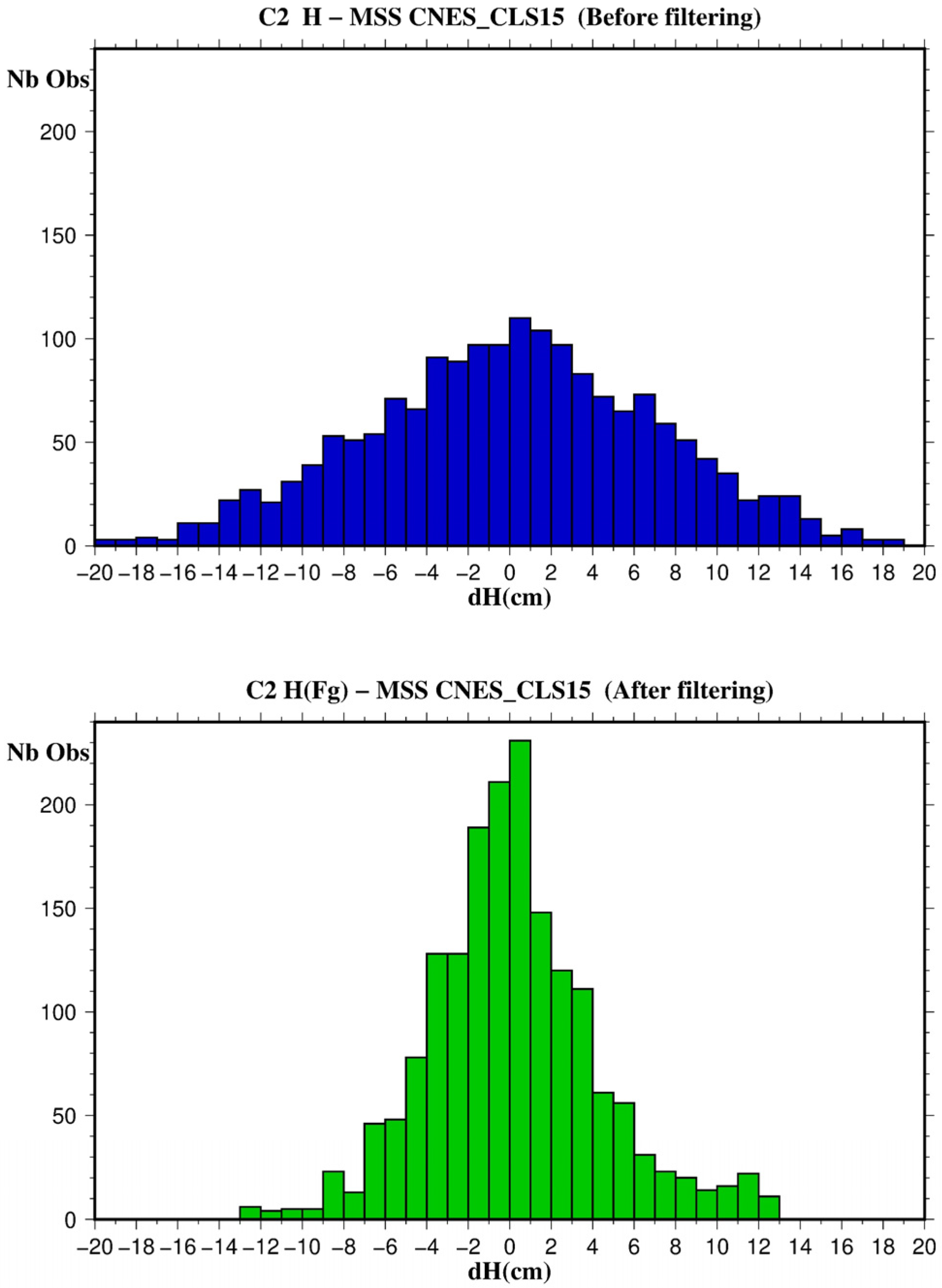
The thin curves correspond to the SSH sampled at 20 Hz and represent the unfiltered difference between the corrected SSH and the CNES_CLS2015 MSS (C2-CLS15). Note that, in this case, the corrected SSH means the application of environmental effects and ocean variability (MSLA). It appears that the noise level of these data sampled at 20 Hz was excessively high to clearly discriminate short-wavelength structures. We therefore used a weighted Gaussian filter with an amplitude of 50% over a distance of 1.6 km to reduce this noise. The result of this filtering is represented by the thick curves (C2(Fg)-CLS15), which clearly provide a better assessment of the topographic content of each profile. In addition, the two histograms in
Figure 5 show the distribution of the data of these two profiles before and after the filtering. We can see that the distribution of the data before the filtering was very spread out, with a standard deviation of 6.8 cm, while the results after filtering appeared more similar to a Gaussian distribution, with a standard deviation of 3.4 cm.
This example is also interesting from another point of view, as it shows that two tracks only a few hundred meters apart can show differences of a few centimeters. Moreover, if we consider the southern parts of these profiles, on the right side of the graph, where we have a relatively flat signal compared to the CNES_CLS 2015 MSS, slight undulations in the order of a centimeter in amplitude can be observed, which may be related to a residual effect of noise after filtering. This led us to introduce correlated Gaussian noise in our covariance matrix, details of which are reported in
Section 3.
Table 1 shows the results of the filtering for the North Pacific region and for a fraction of the cycles used for the C2 and SARAL data. It can be observed that before the filtering, the C2 data had global average biases of around 5.5 cm and standard deviations of 4.0 cm. After the filtering, the data were centered and the standard deviations were homogeneous, with values close to 2.0 cm RMS, for both the C2 and the SARAL. Note that the sampling for the MSS determination was kept at 20 Hz for the C2 and 40 Hz for the SARAL.
2.3. Slope Correction
The objective of slope correction is to take into account the impact of the gradient of the geoid on the range measurement, considering that the point of impact of the return of the radar wave is not at its nadir, but at the closest distance from the radar. Its determination is presented in [
13], where a simple solution is proposed, which is a function of the gradient of the geoid and the altitude of the satellite considered. To apply it, it is only necessary to interpolate a Cartesian grid, which is based on the deviation of the vertical at the position of the satellite considered, and to apply a coefficient corrector, depending on its altitude.
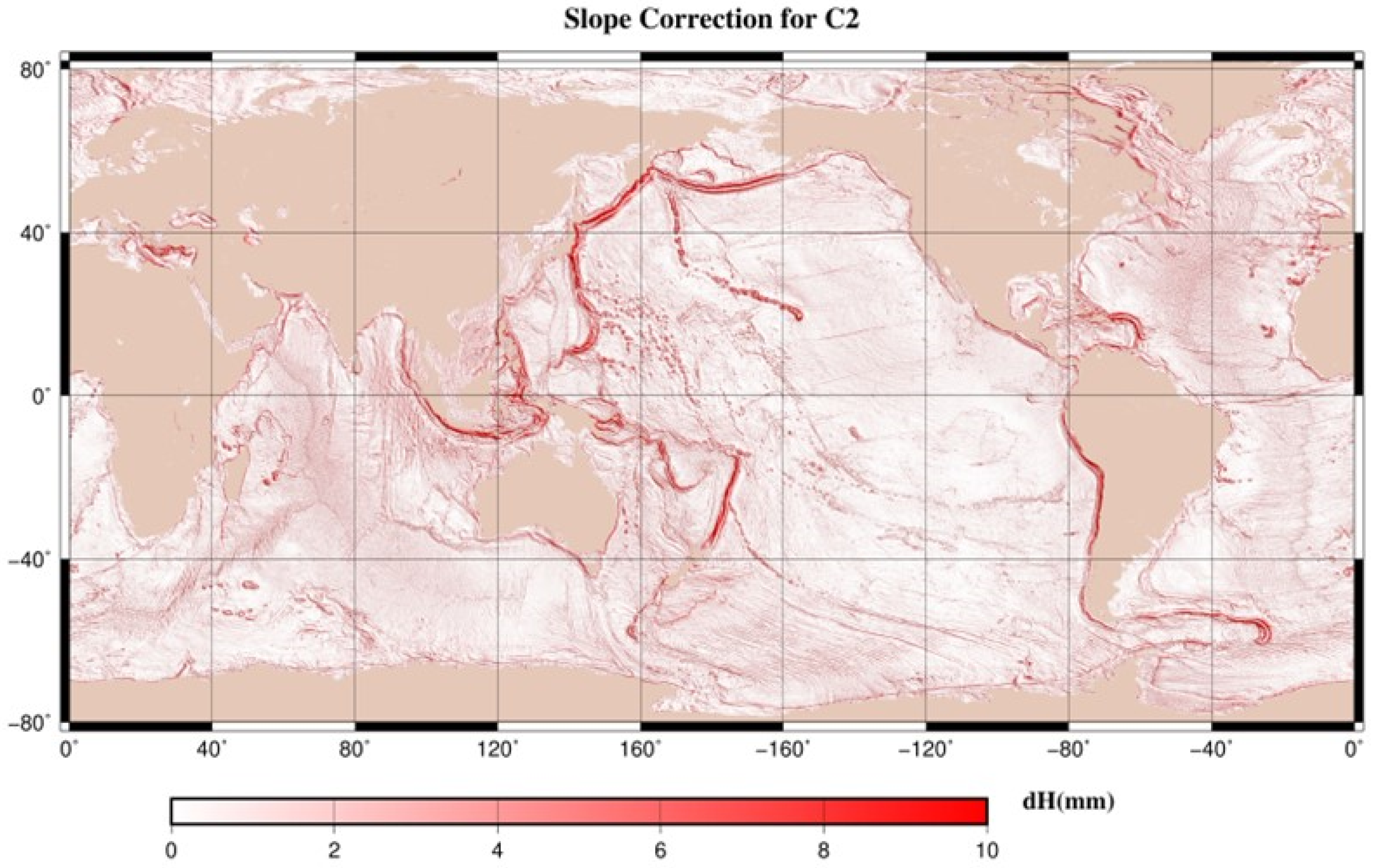
Figure 6 shows the impact of this correction applied to the C2 for an altitude of 725 km. It exceeds values of 10 mm in areas of high geoid slope. In some regions, such as the Aleutian Trench, it can also reach maximum values around 40 mm for C2, while it is 23 mm for a satellite such as Jason-3, with an altitude of 1336 km.
Moreover, considering the improvements in the accuracy of altimetric data in recent years, or, more precisely, the decrease in the instrumental noise at 20 Hz after retracking [
12,
14], for which we can have values of standard deviation between 43 mm and 57 mm for C2 and GeoSat, respectively (except for SARAL with a much lower noise of 29 mm at 40 Hz), it has become important to apply this slope correction to all data that are merged when determining the MSS.
2.4. Altimetric Data for Validation
2.4.1. Open-Ocean and Coastal Data for Validation
Sentinel-3A measurements with 20-Hz sampling were used for the validation of the MSS at short wavelengths in the open ocean. These measurements were selected for two main reasons. The first was that they are independent of the MSS presented in this paper, i.e., the Sentinel-3A measurements were not used for the MSS computation, and they are geographically independent of the measurements used for the MSS computation (i.e., they have a different ground-track position). Furthermore, Sentinel-3A benefits from synthetic aperture radar (SAR) technology. We used the measurements processed with the LR-RMC (low resolution with range-migration-correction) method [
15]. This is an experimental process developed by CNES that significantly reduces the noise at short wavelengths (λ < ~50 km), where conventional SAR processing is known to be affected by sea-state conditions and presents a red noise [
16]. In practice, the measurements were corrected from the different environmental and geophysical corrections, following the same standards as the altimeter measurement used for the MSS computation, and defined in [
10]. We used for the validation of two different cycles of Sentinel-3A measurements: cycles #26 (20 December 2017–16 January 2018) and #38 (9 September 2018, 6 December 2018), which were selected for two periods sufficiently distant in time to decorrelate the oceanic variability [
8]. These data were used to perform the spectral analyses (
Section 4.3) and the coastal validations (
Section 4.4).
2.4.2. Arctic-Leads Sea-Surface-Height Data for Validation
To validate the CNES_CLS 2022 MSS in ice-covered regions (
Section 4.5), we used independent along-track SSH within the leads from the ICESat-2 laser altimetry. The ICESat-2 mission provides high-resolution photon-counting height measurements up to 88°N across its six-beam configuration. The first validation of the sea level in the leads with the conventional Cryosat-2 altimetry were performed [
17]. Here, we used the sea level from the middle strong beam 2R from the ATL07 v5 product [
18], providing sea-level-anomalies referenced to the ICESat-2-product MSS (variable ‘HEIGHT_SEGMENT_HEIGHT’). The product corrections were changed when possible to match the radar-altimeter corrections. These are summarized in
Table 2. Next, three different SLA were referenced to the MSS CNES_CLS 2022, to the MSS DTU15, and to the ICESat-2-product MSS, to quantify the differences between the MSSs.
3. Mapping Method
The mapping method is based on optimal interpolation, also called objective analysis [
19]. The basic principles of the method are described in detail in [
6,
7], and successive improvements are provided in [
5,
8].
In brief, we assume that the best estimate
θest is provided by the following Gauss–Markov linear estimator:
where
= (
λ,
φ) is the location of the estimate,
Aij is the covariance matrix, which is composed of the spatial correlations between the observations (
i, and
j) and their associated uncertainty budget;
Cxj corresponds to the spatial correlations between the estimate and the observations, and
φobs,i are the observations.
The first particularity consists, on one hand, in reliance on the mean profiles of the ERM missions to access the mean oceanic content at the mesoscale and at higher wavelengths, and, on the other hand, in using the high-resolution geodetic (or drifting) missions to map the finest topographic structures down to a resolution of a few km. The ability of this method to improve geophysical structures at the shortest wavelengths strongly depends on the statistical requirements specified by the spatial correlation model (Cxj), as well as the noise budget associated with the observations.
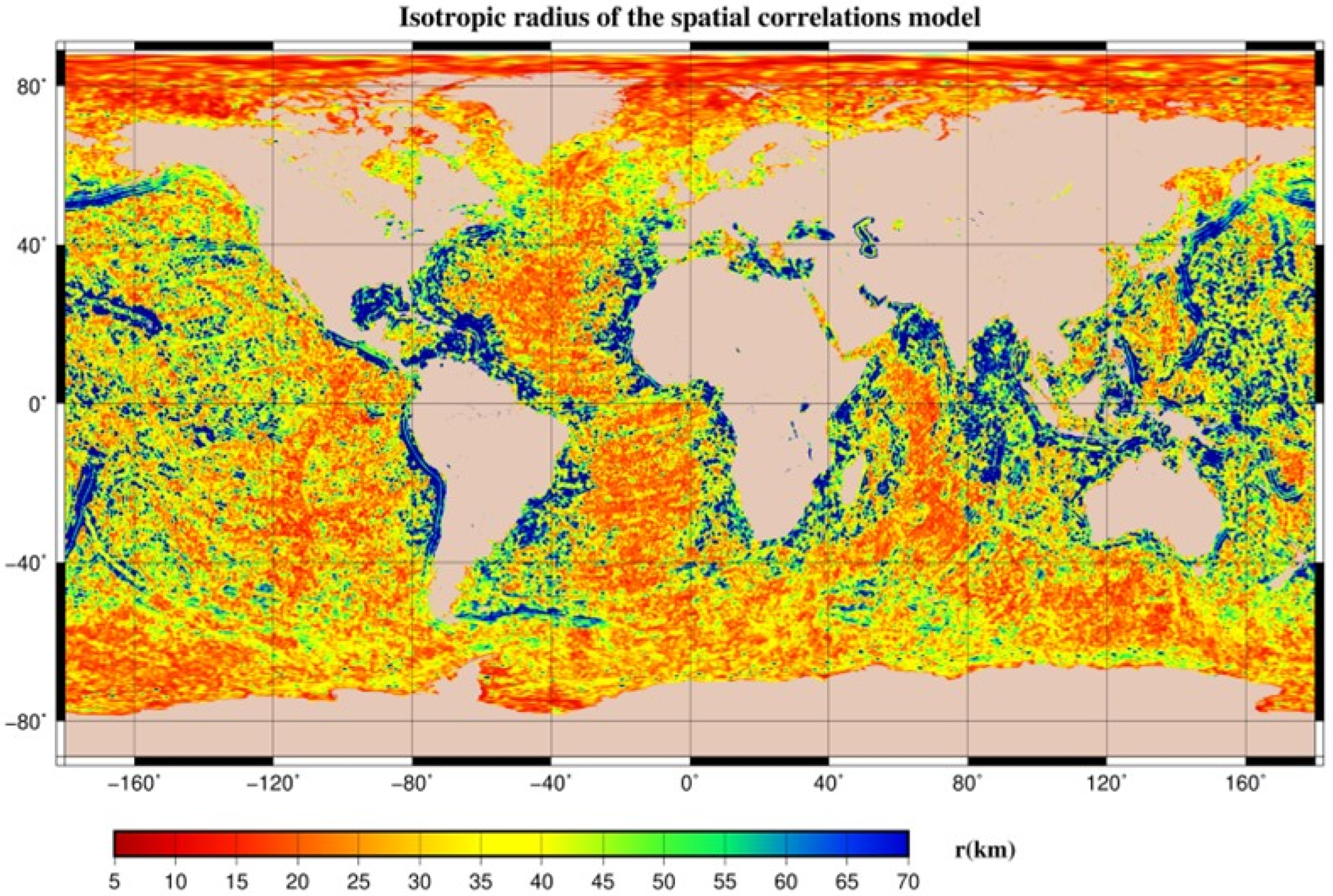
For this MSS, a new correlation model based on the CNES_CLS 2015 MSS was used. Compared to the model that was used for the determination of the previous MSS, which had average radii of about 50 km, the isotropic component of this new model shows radii generally less than 30 km (
Figure 7). In practice, this new model was computed on a 3-min grid with adjusted anisotropic radii in the four cardinal directions.
Another aspect which can drastically improve the accuracy of the results is the noise budget preconized for the observations. Equation (3) represents the error-covariance budget that should be included in the covariance matrix to be inverted. As usual, we use white noise (ɛ) that corresponds to the instrumental noise. Moreover, even if profiles are generally adjusted using least-squares optimization at crossover differences, it residual effects of a few cm can persist between and within altimetric missions. This is why long wavelength errors (B) are also prescribed for wavelengths greater than 300 km. Another very important factor is represented by the third term, which corresponds to the omission error of the residual effect of oceanic variability, especially, as previously explained, for wavelengths below 100 km, which are not fully resolved with the DUACS MSLA fields. The approach used to evaluate this omission error is based on the standard deviation of the mean profiles. We consider, in this case, that it reflects the part of the variability that cannot be assessed.
where:
= (λ,φ) is the position of an observation.
i and j correspond to the indices of the observations.
δij = is the Kronecker symbol, (1 if i = j, 0 otherwise).
ζij = 1 if same track and same satellite.
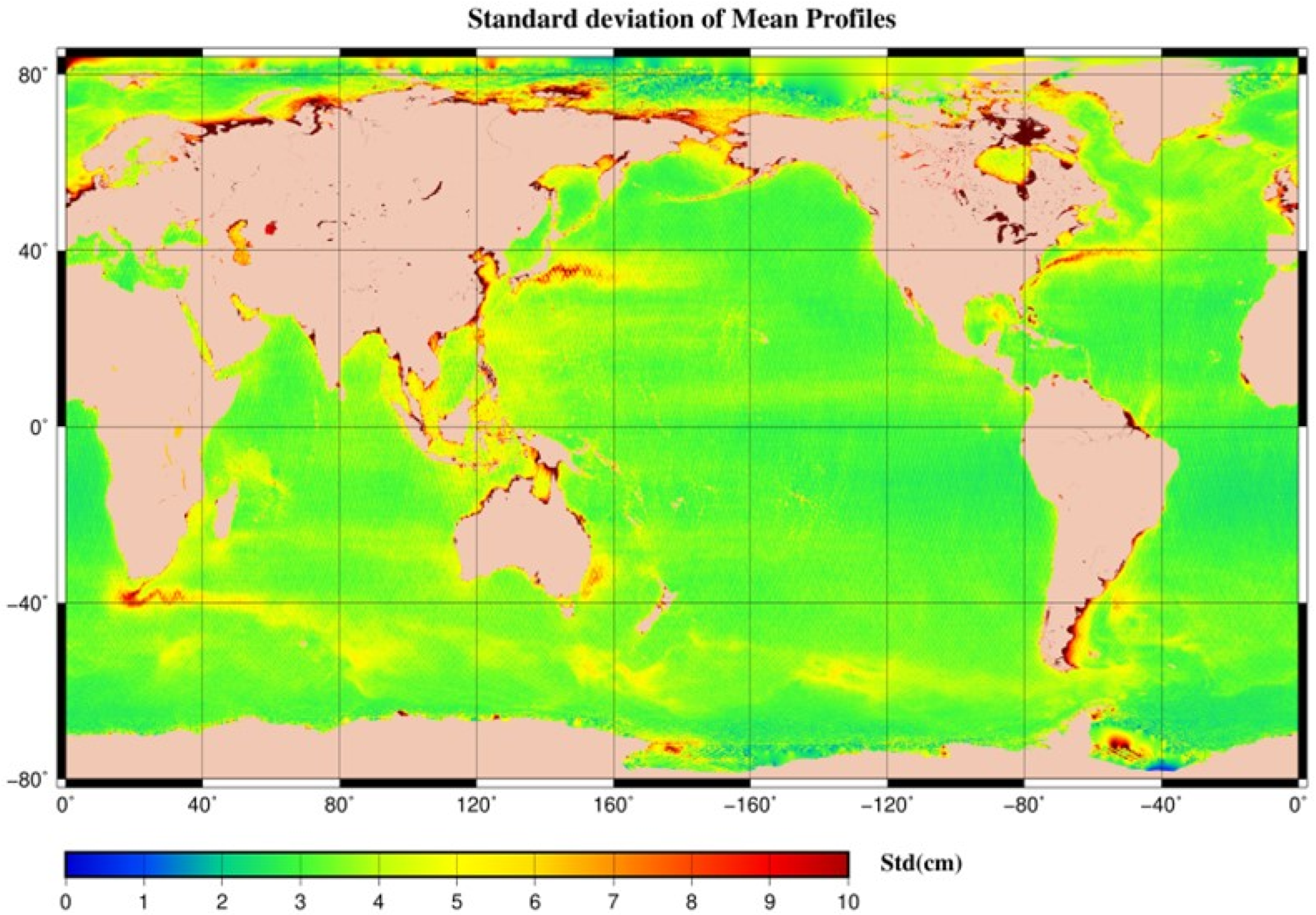
The map in
Figure 8 represents the maximum value of the standard deviation of the mean profiles. This value was computed on a 5-km grid from the standard deviation of the mean heights, which were selected in 100-km-radius bubbles. Next, we assume that the values
Vi and
Vj, which result from the interpolation of this grid, correspond to the uncertainty in our knowledge of the variability at a given position. The
Lvar is a constant that depends on the altimetric mission considered (values of 120 km and 60 km are used for ERM and GM missions respectively). The last term is used to take into account doubts about the residual effect of the Gaussian-filtering processing step described in
Section 2.2, which was only assigned for observations from the same track and the same satellite, where A is a constant corresponding to an amplitude of 1 cm with a correlation length (C) of 5 km.
4. Results
4.1. The CNES_CLS 2022 MSS
The CNES_CLS 2022 MSS was calculated on a 1-min-resolution grid and covered the latitudes between 79.4°S and 88°N. It was completed with the EIGEN 6C4 geoid model [
20] over the continent, and over an area not covered by “valid” altimetric observations. A view of the MSS field is presented in
Figure 9.
The transition between the MSS and the geoid was performed smoothly using a distance-weighted averaging function, and it was implemented only from a threshold within 2.0 cm of the error in order to ensure that we did not affect the MSS, where the accuracy was at the correct level. However, the parallel use of the formal error grid provided with the MSS is recommended to check whether one is located on the MSS or on the geoid. The global field combining the MSS and the geoid is essentially provided for practical purposes for users using Fast Fourier or other transforms or processes.
4.2. Differences between CNES_CLS 2022 and CNES_CLS 2015 MSS
A particularity of our method is that it allows us to obtain an estimate of the formal error, which provides information about the homogeneity of the computed MSS. However, although it is calculated after the adjustment of the noise budget (Equation (3)) with respect to the statistics of the differences at the crossover points, it is not representative of the real error or, more precisely, of the accuracy. In practice, it is rather representative of the relative precision between the different points of the MSS.
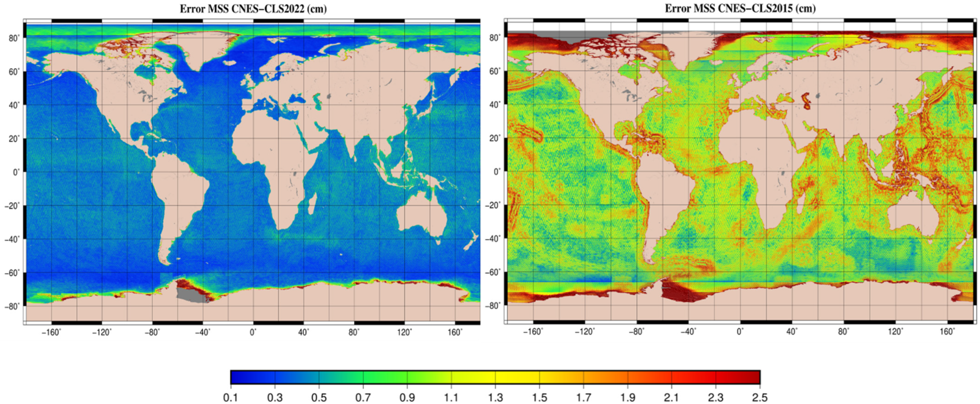
The two maps (
Figure 10) show the formal error of the 2022 and 2015 MSS, respectively. It can be seen that the error of the 2022 MSS is much more homogeneous than that of the 2015 MSS. While, in 2015, the areas with the strongest geoid gradients were more prominent, it is now the areas with strong ocean currents that are most prominent. This logically corresponds to the regions for which there is the most uncertainty, given the difficulty in fully (or perfectly) correcting the data for seasonal and interannual oceanic variability.
From a statistical point of view, the average error, which was 1.4 cm for the 2015 MSS, fells to 0.6 cm for 2022, and the standard deviation was reduced by a factor of two, decreasing from 1.8 cm to 0.9 cm. This improvement was largely due to the number of observations used, 6 billion for the 2022 versus a little more than 200 million for the 2015 MSS. However, the refinement of the spatial correlation model on one hand and of the error covariances on the other also contributed.
Focusing on the 2022 MSS error, we also noted, in Antarctica, an undefined area in gray, for which we had no more valid data. It should be noted that the data for this area were not available at the time we began writing this paper, in 2022, but they are currently under preparation to complement this MSS, as has been the case in the Arctic region. There was also a relatively significant increase in northern Canada, which was due to a substantial loss of valid observations, particularly those of the C2 data, since our processing was not able to handle the SARIn mode.
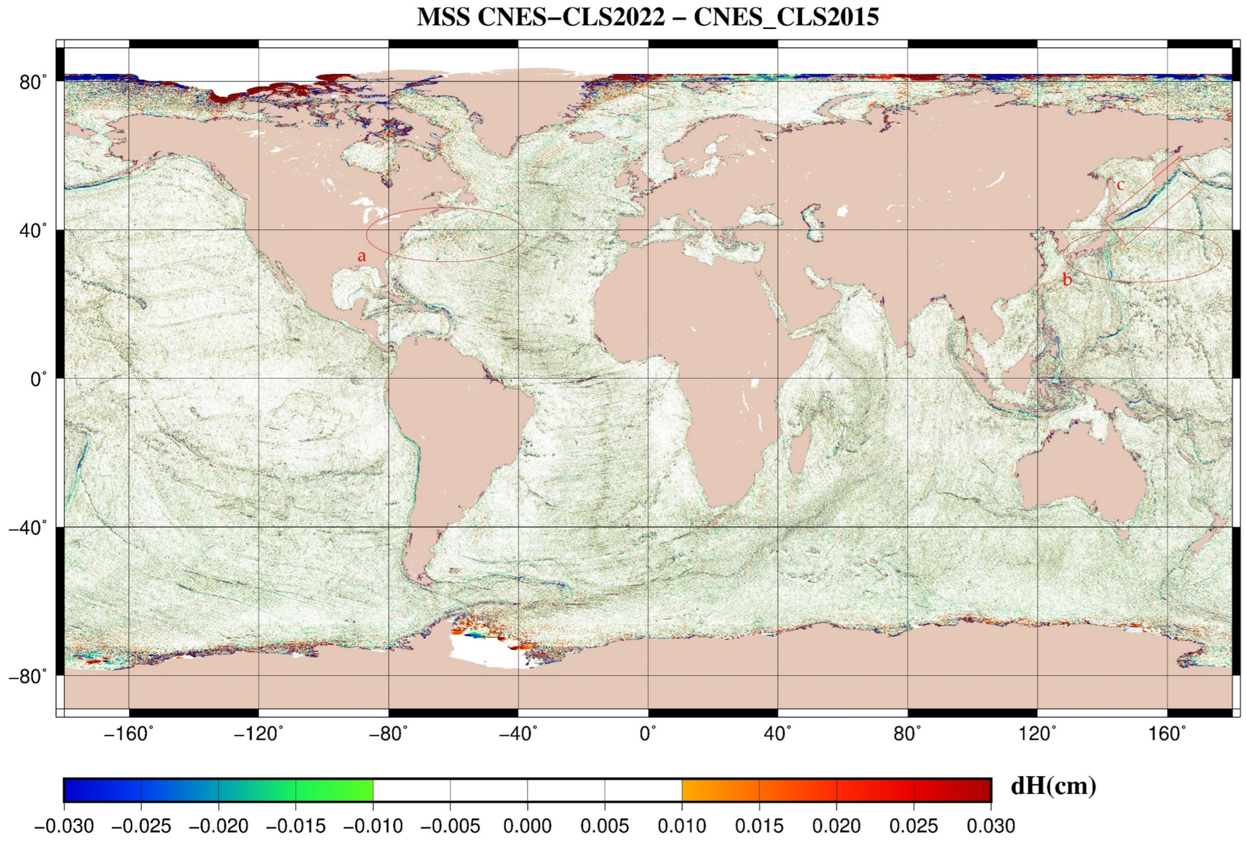
The difference between the MSSs (
Figure 11) provides a first qualitative assessment of the relative content between the MSSs at all the wavelengths. We note that this difference was dominated by short wavelengths, which clearly highlights large bathymetric structures (ridges, fault zones, seamounts). To a minor extent, we noted a slight residual effect over the Gulf Stream (a) and Kuroshio (b) regions, which tended to demonstrate the impact of the improved account of the residual effect of the ocean variability. These improvements are quantified in the next section.
Furthermore, note the negative difference, in blue, along the boundary between the Eurasian and Pacific plates (c), which is related to the implementation of the slope correction (
Section 2.3) for the CNES_CLS 2022 MSS.
From a statistical point of view, the mean difference between these two MSSs was 0.03 cm, with a standard deviation of 2.75 cm. After iterating, with the outliers rejected in differences three times the standard deviation, the mean difference decreased to 1.08 cm and the number of outliers represented 0.8% of all the grid points.
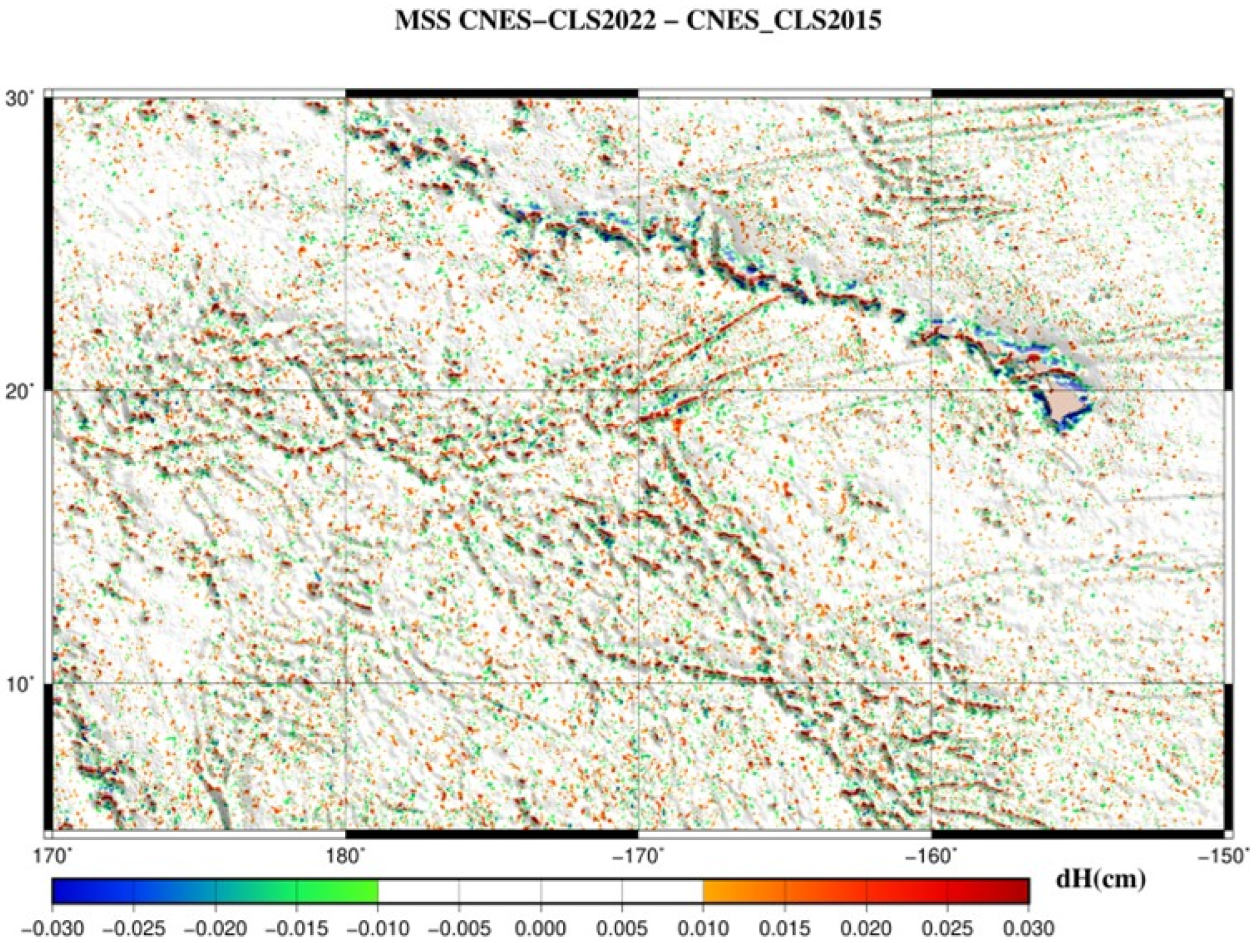
The map (
Figure 12), which is a zoom of this difference over the southwestern Hawaiian Ridge, highlights the refinements obtained at the shortest wavelengths, where the topographic structures, even in the order of 20 km in size, gained in amplitude, with values exceeding 3 cm and reaching 10 cm in some cases.
4.3. MSS Error Estimation at Short Wavelengths
The quantification of the MSS errors at short wavelengths and in the open ocean was performed using the methodology presented in [
8,
21]. In brief, we used the difference between two SLAs (SSH-MSS) from the same track over two cycles, which must be separated in time by several months, the goal being to avoid any correlations in terms of ocean variability. An analysis of the difference in variance between these SLAs then allowed us to decorrelate the errors related to the oceanic variability from that of the MSS. It then became possible to disentangle the dynamical signal from the MSS error.
For this purpose, we used the Sentinel-3A measurement described in
Section 2.3. Cycles #26 and #38 were selected to minimize the correlation of the sea level between these two cycles, which was one of the necessary conditions that allowed us to extract the variance of the MSS error.
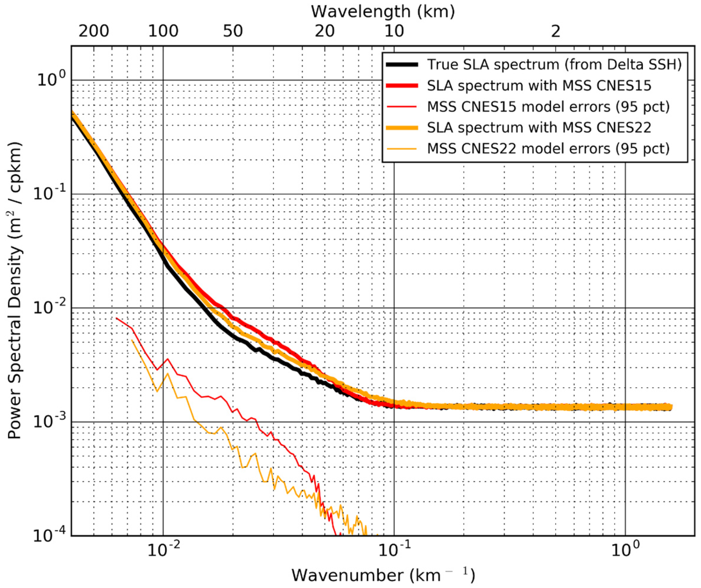
Figure 13 shows the power spectral density (PSD) from which the mean MSS error at short wavelengths (λ < 100 km) was extracted. The black line (the true SLA spectrum) is representative of the SLA unaffected by MSS errors, while the thick colored lines (the SLA spectrum with the CNES15 and CNES22 MSSs) are representative of the SLA including the errors from the two MSSs tested. The half differences between these PSDs are presented by the thin colored lines and represent the error contents of the different MSSs over the wavelength range where this estimation was statistically significant. A reduction is clearly shown in the errors of the CNES_CLS 2022 MSS compared to the CNES_CLS 2015 MSS. The variance of the MSS error over the wavelength ranging from 15 km to 100 km was 0.43 cm
2 for MSS CNES_CLS 2015. It represents around 37% of the “true” SLA variance, i.e., the variance of the SLA without considering the noise instrumental errors. The error of the CNES_CLS 2022 MSS was nearly 0.26 cm
2 (22% of “true” SLA variance), and it was nearly 40% lower than the errors of the previous MSSs.
The spatial distribution of the MSS errors at short wavelengths can be estimated by considering the SLA-error variance in geographical boxes, as presented in [
8,
21].
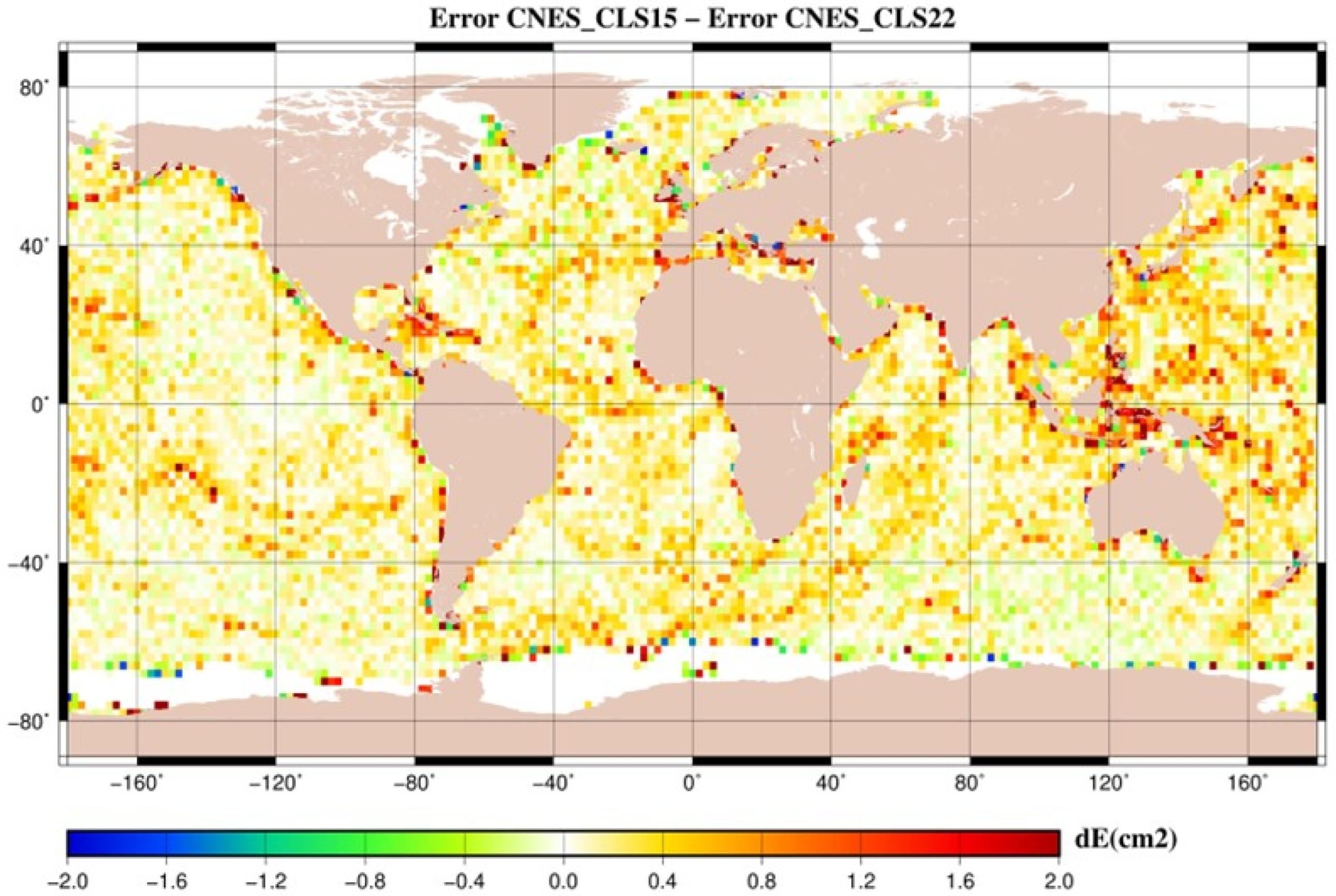
Figure 14 shows the geographical distribution of the MSS-error reduction at short wavelengths when considering the CNES_CLS 2022 rather than the CNES_CLS 2015 version. The figure clearly shows a reduction in errors, mainly located along the geophysical structures with the steepest gradients, where the MSS differences at short wavelengths ere the highest (see
Section 4.1 and
Section 4.2). Locally, the MSS-error reduction reached more than 1 cm
2. The map also underscores the MSS-error reduction near the coast, as discussed in the next section.
4.4. Coastal Areas
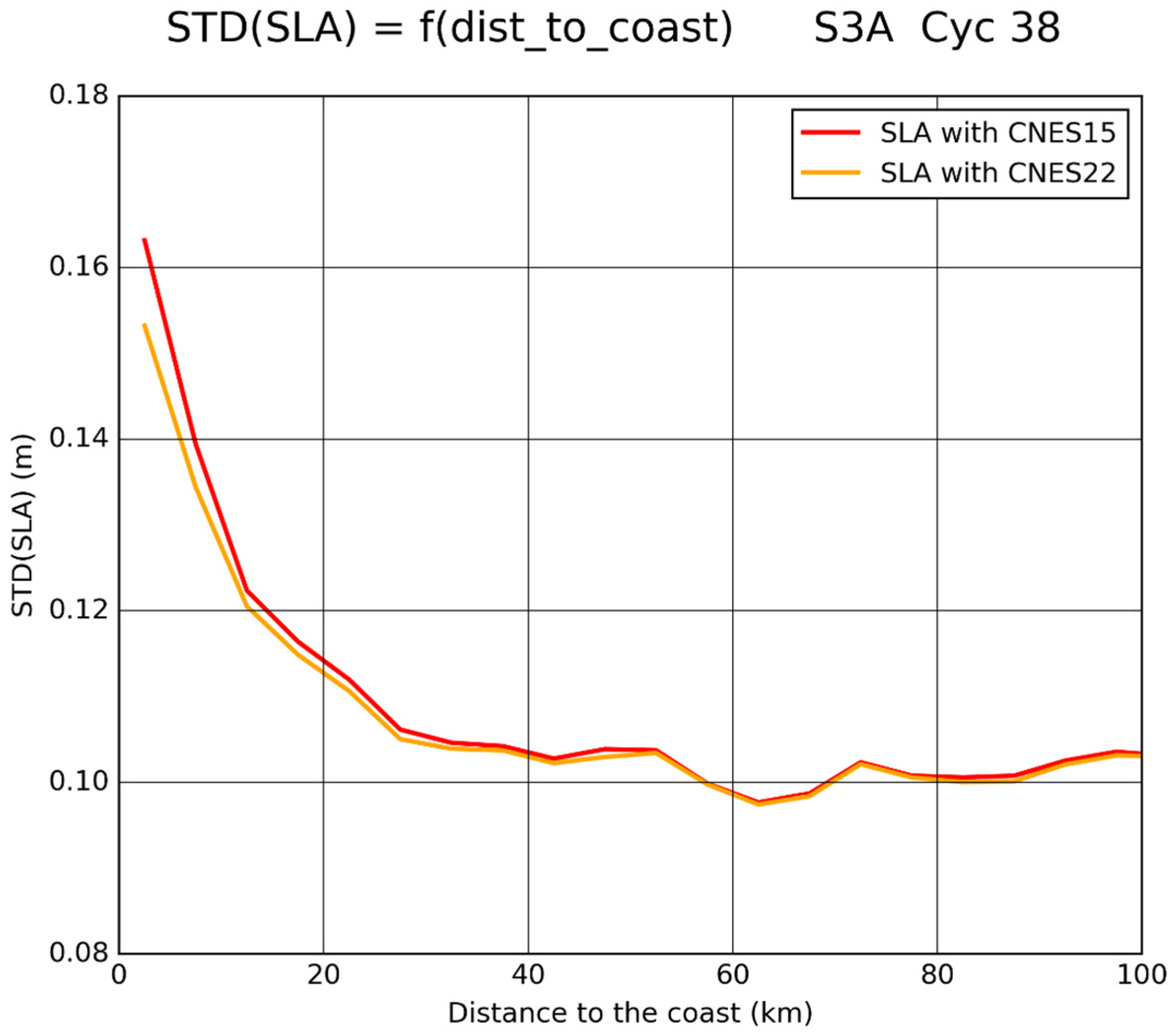
The impact of the MSS in coastal areas was analyzed through the comparison of the standard deviation of the SLA as a function of the distance to the coast.
Figure 15 shows the results obtained with the CNES_CLS 2015 and CNES_CLS_2022 MSSs. It shows the reduced STD of the SLA near the coast with the MSS CNES_CLS 2022. In the 0–5-km bin, the STD of the SLA reduced by 0.53 cm, i.e., a SLA-variance reduction of around 6% compared to the CNES_CLS 2015 results. At 25–30 km, the differences only reached around 2%. Considering the error reduction using the CNES_CLS 2022 MSS compared to the previous version, as quantified in the previous sections, it can be assumed that the SLA STD reduction observed near the coast was mainly induced by the superior accuracy of the CNES_CLS 2022 MSS.
4.5. Arctic Areas
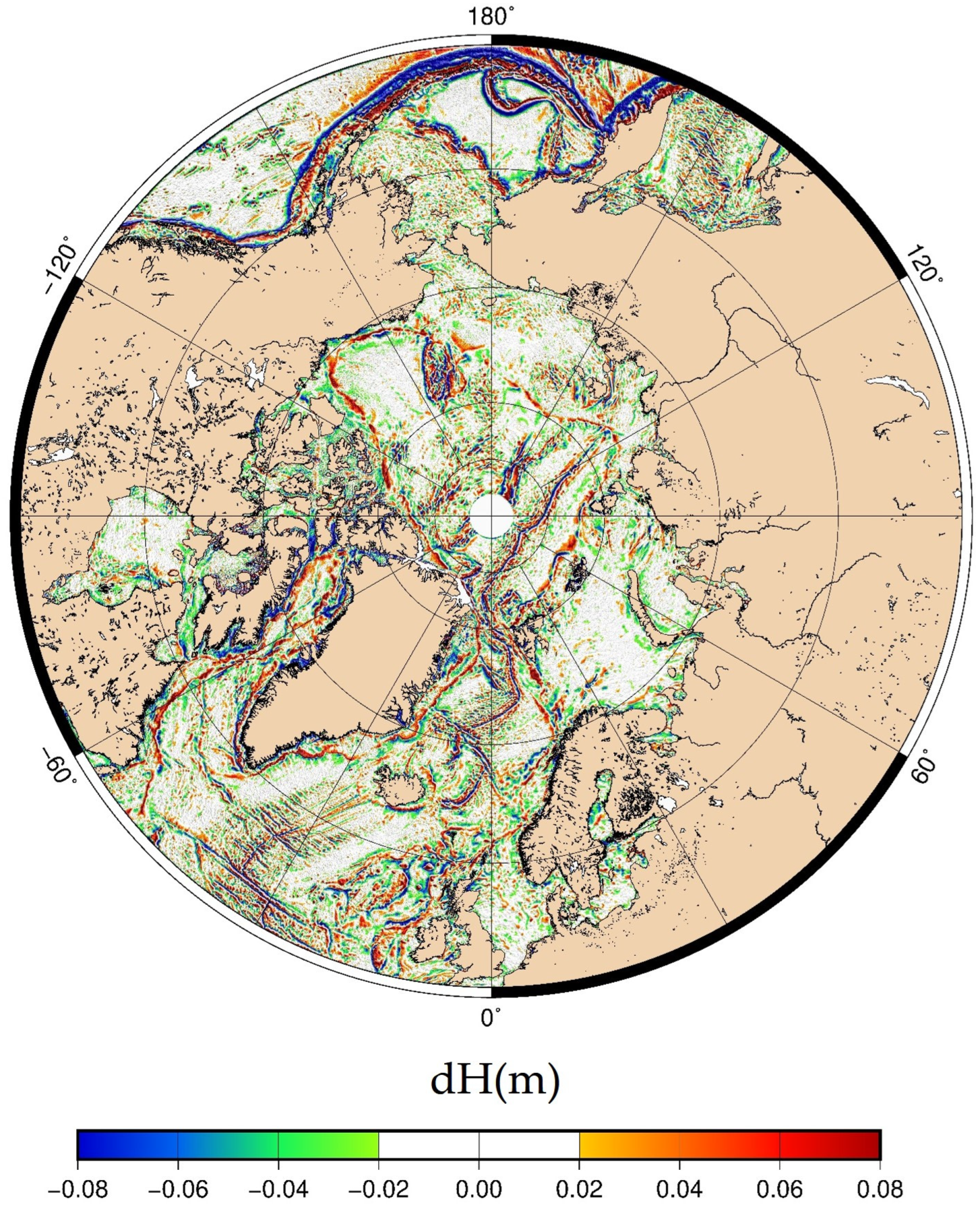
The CNES_CLS 2022 MSS successfully combined the open ocean and the ice-covered Arctic regions. The small-scale features in the Arctic region (
Figure 16) are continuous across the open ocean and the ice-covered regions. The Gakkel and Lomonosov ridges, as well as the Chukchi plateau, are well represented. Other smaller topographic structures are visible.
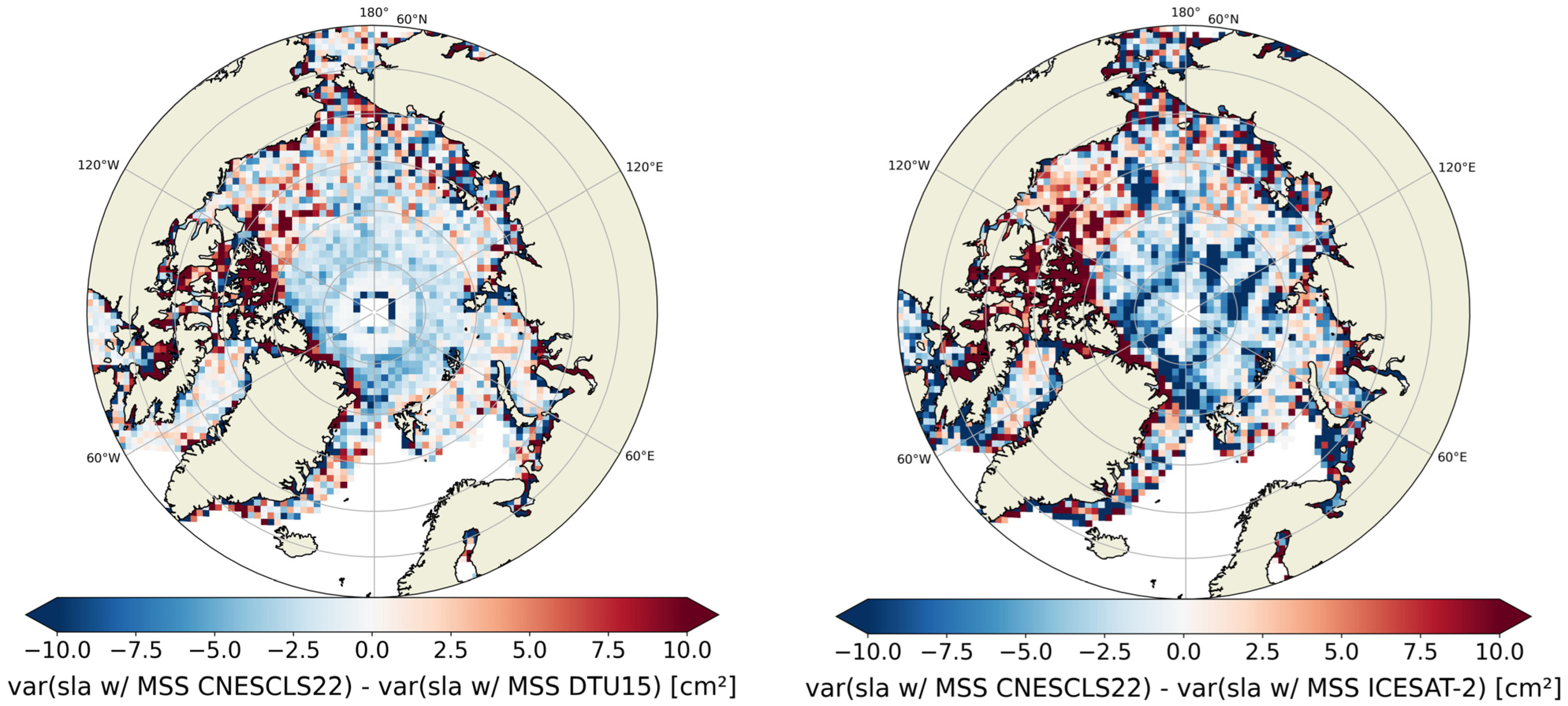
We used sea-level data within the leads from the ICESat-2 laser altimeter to compare this new CNES_CLS 2022 MSS with the DTU15 MSS and the ICESat-2-product MSS in the Arctic region. We compared the variance of the along-track sea-level anomalies corrected with the three MSSs for the period of 14 October 2018 to 30 June 2020. The sea-level variance was reduced with the MSS CNES_CLS 2022 over most of the Arctic region (
Figure 17). The improvement was particularly visible at latitudes over 80°N (
Table 3). Compared to the ICESat-2-product MSS, improvements were visible in the major Arctic topographic structures. Compared to the DTU 2015 MSS, improvements were visible from 80°N to 86°N. However, in coastal regions, the variance increased with the MSS CNES_CLS 2022 compared to the other MSSs. This may have been due to the lack of SARIn C2 data.
5. Conclusions
In this paper, we discussed different factors that can improve the determination of the MSS.
Firstly, we showed that the determination of the MSS is the result of the combination of altimetric missions that provide observations over different periods of time, and that it is essential to correct these data according to seasonal and interannual oceanic variability. To achieve this goal, we found that the use of MSLA DUACS allowed us to homogenize all these SSHs towards a mean height close to the steady state of the ocean.
We also demonstrated that the high-frequency sampling of CryoSat-2 and SARAL/AltiKa altimetric data significantly improved the mapping of the finest topographic structures in the MSS. However, it is necessary to use filtering to reduce the instrumental noise level, and itis important to apply slope correction to ensure better homogeneity between data from different altimeters.
From the point of view of the mapping method, the determination of a new model of the spatial correlations and the improvement of the formalism that takes into account the omission error corresponding to the residual effect of the oceanic variability also contributed to increase the accuracy of the MSS.
In terms of validations, the formal error of the new 2022 MSS is much more homogeneous and decreased by a factor of two compared to the 2015 MSS. From a qualitative point of view, the difference between the 2022 and 2015 MSSs highlights the improvements in the geophysical structures in the shortest wavelengths. Furthermore, the assessment of the error using spectral analysis showed an overall an improvement in the accuracy of this new CNES_CLS 2022 MSS of about 40% compared to the previous model.
Therefore, thanks to new treatments enabling observations over polar areas (sea-ice leads), it is now possible to obtain data with a spatial density and accuracy close to those used for the global ocean. Moreover, the validations carried out with ICESat-2 showed a significant improvement for latitudes higher than 80°N, with a level of precision approaching that obtained in the open ocean.
This new MSS is probably one of the last versions to have been determined solely from conventional nadir altimetric data. It also serves as basis for parallel studies, notably with the Scripps Institution of Oceanography and the Technical University of Denmark, which aims to further refine the shorter wavelengths of the MSS, which should be used as a reference for new swath observations, such as those that will be provided by the SWOT mission.
Author Contributions
Data curation, Q.D., P.V., P.S. and M.-I.P.; formal analysis, P.S., M.-I.P., P.V. and Y.F.; funding acquisition, G.D. and N.P.; writing—original draft, P.S. All authors have read and agreed to the published version of the manuscript.
Funding
This work was financially and technically supported by the French Space Agency (CNES) in the framework of the SALP projects.
Data Availability Statement
Acknowledgments
The generation of the CNES_CLS 2022 MSS model was funded by CNES in the framework of the SWOT and SALP projects. We also thank D. T. Sandwell for the various discussions we had concerning the slope-correction inputs, as well as the improvement in the parameters of the filtering method.
Conflicts of Interest
The authors declare no conflict of interest.
Appendix A
Table A1.
Altimeter missions and periods used to generate the CNES_CLS 2022 MSS version.
Table A1.
Altimeter missions and periods used to generate the CNES_CLS 2022 MSS version.
| Satellite Altimeter Missions | Time Period |
|---|
| Low resolution (1 Hz) |
| Jason-1 + Jason-2 + Jason-3 | May 2002–March 2020 |
| Jason-1 interleaved + Jason-2 interleaved | February 2009–May 2017 |
| GFO | January 2000–August 2008 |
| SARAL/Alika | March 2013–March 2015 |
| High resolution |
| SARAL-DP/ALtiKa (40 Hz) | July 2016–November 2019 (Cycles 100–134) |
| Cryosat-2 (20 Hz) | February 2011–December 2019 (Cycles 14–126) |
Table A2.
Characteristics of the lead along-track data used within the Arctic ice-covered region for the new CNES_CLS 2022 MSS. The environmental and instrumental corrections that differ from the open-ocean DT-2021 processing version are in bold. LRM (low-resolution mode), TFMRA (threshold first-maximum retracker algorithm), DAC (dynamic atmospheric correction).
| | SARAL/AltiKa GDR-F | Sentinel-3A
S3PP | Cryosat-2
Baselines C/D |
|---|
| Latitude max. | 81.5°N | 81.5°N | 88°N |
| Mode | LRM (40 Hz) | SAR (20 Hz) | SAR (20 Hz) |
| Retracking within the leads | Adaptive | TFMRA50 | TFMRA50 |
| Selection | Waveform neural classification + SIC > 90% + sigma0 threshold |
| Env. and Geo. corrections | DAC: MOG2D model (Carrère and Lyard, 2003)
Ocean tide: FES2014 (Carrère et al., 2016)
Pole tide: Desai et al., 2015
Solid Earth tide: Cartwright and Edden, 1973
Ionospheric: GIM (Iijima et al., 1999)
Dry tropospheric: ECMWF model
Wet tropospheric: ECMWF model (on-board radiometer estimates not reliable over ice)
Non-parametric Sea-state bias only over open ocean (waves and wind considered negligible over leads)
MSS: DTU15 (Andersen et al., 2016) |
| SSH | Orbit—Range—∑ Corrections |
References
- Skourup, H.; Farrell, S.L.; Hendricks, S.; Ricker, R.; Armitage, T.W.K.; Ridout, A.; Andersen, O.B.; Haas, C.; Baker, S. An Assessment of State-of-the-Art Mean Sea Surface and Geoid Models of the Arctic Ocean: Implications for Sea Ice Freeboard Retrieval. J. Geophys. Res. Oceans 2017, 122, 8593–8613. [Google Scholar] [CrossRef] [Green Version]
- Andersen, O.B.; Stenseng, L.; Piccioni, G.; Knudsen, P. The DTU15 MSS (mean sea surface) and DTU15LAT (lowest astronomical tide) reference surface. In Proceedings of the ESA Living Planet Symposium, Prague, Czech Republic, 9–13 May 2016. [Google Scholar]
- Prandi, P.; Poisson, J.-C.; Faugère, Y.; Guillot, A.; Dibarboure, G. Arctic sea surface height maps from multi-altimeter combination. Earth Syst. Sci. Data 2021, 13, 5469–5482. [Google Scholar] [CrossRef]
- Rose, S.K.; Andersen, O.B.; Passaro, M.; Ludwigsen, C.A.; Schwatke, C. Arctic Ocean Sea Level Record from the Complete Radar Altimetry Era: 1991–2018. Remote Sens. 2019, 11, 1672. [Google Scholar] [CrossRef] [Green Version]
- Schaeffer, P.; Faugére, Y.; Legeais, J.F.; Ollivier, A.; Guinle, T.; Picot, N. The CNES_CLS11 Global Mean Sea Surface Computed from 16 Years of Satellite Altimeter Data. Mar. Geodesy 2012, 35, 3–19. [Google Scholar] [CrossRef]
- Hernandez, F.; Schaeffer, P.; Calvez, M.H.; Dorandeu, J.; Faugére, Y.; Mertz, F. Surface Moyenne Oceanique: Support Scientifique à la Mission Altimetrique Jason-1, et à Une Mission Microsatellite, Altimétrique; Contract SSALTO 2945–Ot2–A. 1. Rapport final n CLS. DOS/NT/00.341; CLS: Ramonville St Agne, France, 2001. [Google Scholar]
- Hernandez, F.; Schaeffer, P. Altimetric Mean Sea Surfaces and Gravity Anomaly Maps Inter-Comparisons; AVISO Tech. Rep. AVI-NT-011-5242-CLS, Cent. Natl; d’Etudes Spatiales: Toulouse, France, 2002. [Google Scholar]
- Pujol, M.-I.; Schaeffer, P.; Faugère, Y.; Raynal, M.; Dibarboure, G.; Picot, N. Gauging the Improvement of Recent Mean Sea Surface Models: A New Approach for Identifying and Quantifying Their Errors. J. Geophys. Res. Oceans 2018, 123, 5889–5911. [Google Scholar] [CrossRef]
- Ballarotta, M.; Ubelmann, C.; Pujol, M.-I.; Taburet, G.; Fournier, F.; Legeais, J.-F.; Faugère, Y.; Delepoulle, A.; Chelton, D.; Dibarboure, G.; et al. On the resolutions of ocean altimetry maps. Ocean Sci. 2019, 15, 1091–1109. [Google Scholar] [CrossRef] [Green Version]
- Lievin, M.; Kocha, C.; Courcol, B.; Philipps, S.; Denis, I.; Guinle, T. Reprocessing of Sea Level L2P Products for 28 Years of Altimetry Missions. Présenté à OSTST, 2020. Available online: https://ostst.aviso.altimetry.fr/fileadmin/user_upload/tx_ausyclsseminar/files/OSTST2020_Reprocessing_L2P_2020.pdf (accessed on 3 April 2023).
- Taburet, G.; Sanchez-Roman, A.; Ballarotta, M.; Pujol, M.-I.; Legeais, J.-F.; Fournier, F.; Faugere, Y.; Dibarboure, G. DUACS DT2018: 25 years of reprocessed sea level altimetry products. Ocean Sci. 2019, 15, 1207–1224. [Google Scholar] [CrossRef] [Green Version]
- Zhang, S.; Sandwell, D.T. Retracking of SARAL/AltiKa radar altimetry waveforms for optimal gravity field recovery. Mar. Geodesy 2017, 40, 40–56. [Google Scholar] [CrossRef]
- Sandwell, D.T.; Smith, W.H.F. Slope correction for ocean radar altimetry. J. Geod. 2014, 88, 765–771. [Google Scholar] [CrossRef]
- Garcia, E.S.; Sandwell, D.; Smith, W. Retracking CryoSat-2, Envisat and Jason-1 radar altimetry waveforms for improved gravity field recovery. Geophys. J. Int. 2014, 196, 1402–1422. [Google Scholar] [CrossRef] [Green Version]
- Moreau, T.; Cadier, E.; Boy, F.; Aublanc, J.; Rieu, P.; Raynal, M.; Labroue, S.; Thibaut, P.; Dibarboure, G.; Picot, N.; et al. High-performance altimeter Doppler processing for measuring sea level height under varying sea state conditions. Adv. Space Res. 2021, 67, 1870–1886. [Google Scholar] [CrossRef]
- Rieu, P.; Moreau, T.; Cadier, E.; Raynal, M.; Clerc, S.; Donlon, C.; Borde, F.; Boy, F.; Maraldi, C. Exploiting the Sentinel-3 tandem phase dataset and azimuth oversampling to better characterize the sensitivity of SAR altimeter sea surface height to long ocean waves. Adv. Space Res. 2020, 67, 253–265. [Google Scholar] [CrossRef]
- Bagnardi, M.; Kurtz, N.T.; Petty, A.A.; Kwok, R. Sea Surface Height Anomalies of the Arctic Ocean from ICESat-2: A First Examination and Comparisons with CryoSat-2. Geophys. Res. Lett. 2021, 48, e2021GL093155. [Google Scholar] [CrossRef]
- Kwok, R.; Cunningham, G.; Markus, T.; Hancock, D.; Morison, J.; Palm, S.; Farrell, S.L.; Ivanoff, A.; Wimert, J. ATLAS/ICESat-2 L3A Sea Ice Height, Version 5 [Data Set]. 2021. Available online: https://nsidc.org/data/atl07/versions/5 (accessed on 3 April 2023).
- Bretherton, F.P.; Davis, R.E.; Fandry, C. A technique for objective analysis and design of oceanographic experiments applied to MODE-73. Deep. Sea Res. Oceanogr. Abstr. 1976, 23, 559–582. [Google Scholar] [CrossRef]
- Ch, F.; Bruinsma, S.L.; Abrikosov, O.; Lemoine, J.M.; Schaller, T.; Gtze, H.J.; Ebbing, J.; Marty, J.C.; Flechtner, F.; Balmino, G.; et al. EIGEN-6C4 The Latest Combined Global Gravity Field Model including GOCE Data up to Degree and Order 2190 of GFZ Potsdam and GRGS Toulouse. GFZ Data Services. 2014. Available online: https://dataservices.gfz-potsdam.de/icgem/showshort.php?id=escidoc:1119897 (accessed on 3 April 2023).
- Dibarboure, G.; Pujol, M.-I. Improving the quality of Sentinel-3A data with a hybrid mean sea surface model, and implications for Sentinel-3B and SWOT. Adv. Space Res. 2021, 68, 1116–1139. [Google Scholar] [CrossRef]
Figure 1.
Overview of the altimetric missions used and their temporal coverage. TP (Topex/Poseidon), J (Jason 1, 2, 3), E1 (ERS-1), E2 (ERS-2), En (EnviSat), GFO (GeoSat Follow-On), C2 (CryoSat-2), SARAL (SARAL/AltiKa).
Figure 1.
Overview of the altimetric missions used and their temporal coverage. TP (Topex/Poseidon), J (Jason 1, 2, 3), E1 (ERS-1), E2 (ERS-2), En (EnviSat), GFO (GeoSat Follow-On), C2 (CryoSat-2), SARAL (SARAL/AltiKa).
Figure 2.
SLA evolution over time, calculated from DUACS SLA products.
Figure 2.
SLA evolution over time, calculated from DUACS SLA products.
Figure 3.
Average multi-mission DUACS gridded products over the MSS reference period [1993, 2012]. Note that here, the average bias of 2.6 cm is removed. Residual effect in Gulf Stream (a), Agulhas Current (b), Kuroshio (c), and high latitudes (d,e).
Figure 3.
Average multi-mission DUACS gridded products over the MSS reference period [1993, 2012]. Note that here, the average bias of 2.6 cm is removed. Residual effect in Gulf Stream (a), Agulhas Current (b), Kuroshio (c), and high latitudes (d,e).
Figure 4.
Cross view of CryoSat-2 profiles. Track #49509 (red curve), Track #62277 (blue curve).
Figure 4.
Cross view of CryoSat-2 profiles. Track #49509 (red curve), Track #62277 (blue curve).
Figure 5.
Histogram of C2 before/after filtering.
Figure 5.
Histogram of C2 before/after filtering.
Figure 6.
Slope correction applied to CryoSat-2.
Figure 6.
Slope correction applied to CryoSat-2.
Figure 7.
Isotropic radius of the correlation model used for the CNES_CLS 2022 MSS determination.
Figure 7.
Isotropic radius of the correlation model used for the CNES_CLS 2022 MSS determination.
Figure 8.
Uncertainties over the residual effect of the oceanic variability calculated from the standard deviation of mean profile heights.
Figure 8.
Uncertainties over the residual effect of the oceanic variability calculated from the standard deviation of mean profile heights.
Figure 9.
Global mean sea surface CNES_CLS 2022.
Figure 9.
Global mean sea surface CNES_CLS 2022.
Figure 10.
Error of CNES_CLS 2022 and 2015 MSS. E (cm).
Figure 10.
Error of CNES_CLS 2022 and 2015 MSS. E (cm).
Figure 11.
Differences between CNES_CLS 2022 and CNES_CLS 2015 MSS. Oceanic residual effect over the Gulf Stream (a) and Kuroshio (b) regions. Impact of implementation of the slope correction (c).
Figure 11.
Differences between CNES_CLS 2022 and CNES_CLS 2015 MSS. Oceanic residual effect over the Gulf Stream (a) and Kuroshio (b) regions. Impact of implementation of the slope correction (c).
Figure 12.
Zoom of MSS difference near the Hawaiian Ridge.
Figure 12.
Zoom of MSS difference near the Hawaiian Ridge.
Figure 13.
Power spectral density (PSD) of the half-difference of Sentinel-3 SSH from cycle 26 and cycle 38 (thick black line). PSD of the sea-level anomaly (half-mean of cycle 26 and cycle 38) computed with the various MSS references (thick colored lines). PSD of the MSS errors (thin colored lines) where statistically significant (95% confidence threshold).
Figure 14.
Map of the differences between the errors of CNES_CLS 2015 and CNES_CLS 2022 MSS for wavelengths ranging from 15 km to 100 km. Positive values mean lower errors for CNES_CLS 2022 MSS solution.
Figure 14.
Map of the differences between the errors of CNES_CLS 2015 and CNES_CLS 2022 MSS for wavelengths ranging from 15 km to 100 km. Positive values mean lower errors for CNES_CLS 2022 MSS solution.
Figure 15.
Standard deviation of the SLA as a function of the distance to the closest shoreline position (5-km bins). SLA computed with CNES_CLS 2015 (red line) and CNES_CLS 2022 (orange line) MSS.
Figure 15.
Standard deviation of the SLA as a function of the distance to the closest shoreline position (5-km bins). SLA computed with CNES_CLS 2015 (red line) and CNES_CLS 2022 (orange line) MSS.
Figure 16.
Small-scale features (λ < 50km) of the MSS CNES_CLS 2022 in the Arctic area.
Figure 16.
Small-scale features (λ < 50km) of the MSS CNES_CLS 2022 in the Arctic area.
Figure 17.
Differences in variance of sea level corrected with the MSS CNES_CLS 2022 and with the DTU 2015 MSS in 50-km boxes for the period of October 2018 to June 2020 (left). with the same applies to the MSS CNES_CLS 2022 and with the ICESat-2-product MSS (right).
Figure 17.
Differences in variance of sea level corrected with the MSS CNES_CLS 2022 and with the DTU 2015 MSS in 50-km boxes for the period of October 2018 to June 2020 (left). with the same applies to the MSS CNES_CLS 2022 and with the ICESat-2-product MSS (right).
Table 1.
Filtering statistics: H corresponds to SSH, H_Fg to the filtered height, and CLS15 to the CNES_CLS15 MSS.
Table 1.
Filtering statistics: H corresponds to SSH, H_Fg to the filtered height, and CLS15 to the CNES_CLS15 MSS.
| Nbr Obs | Average | Std | RMS | dH (m) |
|---|
| C2 PDGS (20 Hz) cycles 14–36 |
| 122 716 126 | −0.056 | 0.039 | 0.068 | H-CLS15 |
| 122 716 122 | 0.000 | 0,020 | 0.020 | H_Fg-CLS15 |
| C2 PDGS (20 Hz) cycles 97–116 |
| 110 434 652 | −0.055 | 0.041 | 0.068 | H-CLS15 |
| 110 434 652 | 0.000 | 0.021 | 0.021 | H_Fg-CLS15 |
| AltiKa (40 Hz) |
| 371 560 919 | −0.007 | 0.041 | 0.042 | H-CLS15 |
| 371 560 632 | 0.000 | 0.019 | 0.019 | H_Fg-CLS15 |
Table 2.
Corrections applied to ICESat-2 lead data.
Table 2.
Corrections applied to ICESat-2 lead data.
| | Model: |
|---|
| Solid Earth Tide | Cartwright model |
Ocean Loading, Tide,
and Long-Period-Equilib. Tide | FES2022B model |
| Solid-Earth-Pole Tide | Not applied |
| Ocean-Pole Tide | ICESAT-2 correction |
| DAC | MOG2D HR |
| Total column atm. delay | Luthcke and Petrov, ATBD ATL03a |
Table 3.
Reduction in variance of the CNES_CLS 2022 MSS compared to DTU 2015 MSS and the MSS from the ICESat-2 product.
Table 3.
Reduction in variance of the CNES_CLS 2022 MSS compared to DTU 2015 MSS and the MSS from the ICESat-2 product.
| | Entire Region | Excluding Coastal Region (>100 km) | For Latitudes >80°N, Excluding Coastal Region |
|---|
| Var(sla w/MSS CNES/CLS22)—Var(sla w/MSS DTU15) | +0.5% | −2% | −11% |
| Var(sla w/MSS CNES/CLS22)—Var(sla w/ICESat-2 product MSS) | −61% | −81% | −92% |
| Disclaimer/Publisher’s Note: The statements, opinions and data contained in all publications are solely those of the individual author(s) and contributor(s) and not of MDPI and/or the editor(s). MDPI and/or the editor(s) disclaim responsibility for any injury to people or property resulting from any ideas, methods, instructions or products referred to in the content. |
© 2023 by the authors. Licensee MDPI, Basel, Switzerland. This article is an open access article distributed under the terms and conditions of the Creative Commons Attribution (CC BY) license (https://creativecommons.org/licenses/by/4.0/).


 ,
, 


