Article

Ionospheric–Thermospheric Responses to Geomagnetic Storms from Multi-Instrument Space Weather Data

1
Department of Space Sciences, GNSS and Space Education Lab, National Center of GIS and Space Application, Institute of Space Technology, Islamabad 44000, Pakistan
2
Key Laboratory of Earth and Planetary Physics, Institute of Geology and Geophysics, Chinese Academy of Sciences, Beijing 100045, China
3
Centre for Earthquake Studies, National Centre for Physics, Islamabad 44000, Pakistan
4
College of Earth and Planetary Sciences, University of Chinese Academy of Sciences, Beijing 100049, China
5
Department of Physics and Mathematics, University of Alcalá de Henares, 28031 Madrid, Spain
6
SCiESMEX, LANCE, Instituto de Geofísica, Unidad Michoacán, Universidad Nacional Autónoma de México, Morelia C.P. 58089, Michoacán, Mexico
7
King Mongkut’s Institute of Technology Ladkrabang, Prince of Chumphon Campus, Chumphon 86160, Thailand
8
Heilongjiang Mohe Observatory of Geophysics, Institute of Geology and Geophysics, Chinese Academy of Sciences, Beijing 100045, China
*
Author to whom correspondence should be addressed.
These authors contributed equally to this work.
Remote Sens. 2023, 15(10), 2687; https://doi.org/10.3390/rs15102687
Submission received: 7 April 2023 / Revised: 11 May 2023 / Accepted: 12 May 2023 / Published: 22 May 2023
(This article belongs to the Special Issue Satellite Observations of the Global Ionosphere and Plasma Dynamics)

Abstract

:
We analyze vertical total electron content (vTEC) variations from the Global Navigation Satellite System (GNSS) at different latitudes in different continents of the world during the geomagnetic storms of June 2015, August 2018, and November 2021. The resulting ionospheric perturbations at the low and mid-latitudes are investigated in terms of the prompt penetration electric field (PPEF), the equatorial electrojet (EEJ), and the magnetic H component from INTERMAGNET stations near the equator. East and Southeast Asia, Russia, and Oceania exhibited positive vTEC disturbances, while South American stations showed negative vTEC disturbances during all the storms. We also analyzed the vTEC from the Swarm satellites and found similar results to the retrieved vTEC data during the June 2015 and August 2018 storms. Moreover, we observed that ionospheric plasma tended to increase rapidly during the local afternoon in the main phase of the storms and has the opposite behavior at nighttime. The equatorial ionization anomaly (EIA) crest expansion to higher latitudes is driven by PPEF during daytime at the main and recovery phases of the storms. The magnetic H component exhibits longitudinal behavior along with the EEJ enhancement near the magnetic equator.

Graphical Abstract

1. Introduction

The Sun triggers space weather events such as geomagnetic storms that can cause negative impacts on the communication and navigation through transionospheric electromagnetic signals on the Earth. Geomagnetic storms result from large-scale disturbances of the Earth’s magnetosphere under variable solar activity, leading to anomalous ionosphere variability. These disturbances occur at short-term scales (hours to a few days). They are usually triggered by coronal mass ejection (CME), co-rotating interaction regions (CIRs), or fast-moving solar wind streams. Anomalous ionospheric variations were observed from plasma content variability during the geomagnetic storms of 6 April and 29 May 2010 [1,2]. Several studies have investigated the ionospheric variations during storms at different latitudes from satellite data [3,4,5]. Seasonal variations and hemispheric ionospheric irregularities are also present during geomagnetic storms [6,7,8,9]. The upper atmosphere is subjected to a significant amount of energy due to highly dynamic solar winds during major events enhancing the high-latitude convection electric field. This further leads to enhancement of joule heating and temperature of thermosphere as a large velocity gap is created between the ions and neutrals [10,11]. Due to this, horizontal winds are also subjected to perturbations as both ion drag increases along with variations in horizontal pressure gradient [12]. This creates atmospheric upwelling accompanied by compositional changes at high latitudes that are then carried towards lower latitude by horizontal winds and travelling ionospheric disturbance waves [13,14,15]. As a result, the storm-time change in circulation redistributes thermospheric energy, momentum, and composition globally and significantly impacts the ionosphere [11,12,16]. However, the overall perception of storm-time ionospheric–thermospheric variations across the different latitude ranges in both hemispheres is still uncertain.
GNSS-based total electron content (TEC) and in situ data from multiple instruments describe the ionospheric abnormalities in different spatial and temporal resolutions at different latitudes during active solar and geomagnetic conditions [17]. Transionospheric signal delay during storm conditions results in unacceptable GNSS positioning errors for practical applications [18,19,20,21]. Since the ionospheric delay in GNSS signals is not yet corrected, the Global Ionospheric Maps (GIMs) of TEC from the International GNSS Service (IGS) are an exceptional product to calibrate the ionospheric correction and eliminate discrepancies from GNSS signals with the help of other multi-instrument data.
Geomagnetic storms induce effects in the ionosphere at different latitudes and longitudes in the form of electric field penetration from high to low latitudes due to PPEF. Furthermore, the perturbations of global thermospheric circulation at high latitudes induce joule-heating enhancement during geomagnetic activity, leading to disturbed dynamo electric fields (DDEFs). At equatorial and low latitudes, the electrodynamics in the ionospheric E and F regions influence the plasma distribution [22]. A field-aligned current system (FACS) controls the transfer of energy and momentum from the magnetosphere to the ionosphere in the form of two clear shells [23]. These two shells include regions 1 and 2 for higher and lower latitudes connected through the ionosphere around the Earth, respectively. The neutral wind dynamo induces polarized electric fields in the low latitude during the dayside (nightside) in an eastward (westward) direction [24]. The horizontal magnetic field component corresponds to the zonal electric field generating electron upwelling due to the E×B effect. As a result, negatively and positively charged particles form on the top and bottom of the ionospheric E region, respectively. At an altitude of 90–130 km, the migration of electrons produces an electric current known as the equatorial electrojet (EEJ).
Sharma et al. [25] presented two enhanced peaks in TEC with twice the intensity of quiet days in low latitude regions as storm-time responses. They showed that the first peak in ionospheric TEC was due to PPEF, and the second peak occurred due to plasma fountain. Moreover, the PPEF influences along the longitudes showed nearly homogeneous effects in the storm of 25 August 2005. On the other hand, the southward-shifted interplanetary magnetic field (IMF) Bz component induced increased activity in high-latitude convection. Previous findings have provided insights on mid-latitude TEC enhancements during the initial phase of geomagnetic storms compared to the main phase [26,27]. For example, Astafyeva et al. [28] showed the equatorial and mid-latitudinal ionospheric TEC during the main phase of the storm in a different part of the world from multi-instrument satellite data. Similarly, Astafyeva et al. [29] assessed the effects of the June 2015 geomagnetic storm with a comprehensive study using multiple satellite observations. They demonstrated that the storm had major effects on the ionosphere due to thermospheric winds in the low and mid-latitude regions. They also showed that dayside neutral mass density enhancement during storms exceeded the quiet period in the thermosphere due to robust PPEF influencing the ionosphere with significant variability. Moreover, Adebiyi et al. [1] and Joshua et al. [2] reported enhanced electron density in the African equatorial region during the geomagnetic storms of 6 April and 29 May 2010.
Apart from the above reports, positive and negative ionospheric anomalies due to geomagnetic storms can vary significantly, depending on the duration of the solar activity, season, latitude, local solar time, etc., and each storm shows different characteristics. We need to observe satellite data with multiple instruments in order to find the missing drivers [27,30]. This study comprises understanding the probable latitudinal mechanisms that influence the variable ionosphere by studying the geomagnetic storms of June 2015, August 2018 and November 2021 using multi-instrumental data. This paper examines the global morphology of the geomagnetic storms using multi-instrument and multi-parameter approaches to analyze the behavior of various atmospheric layers of Earth. In the following section, we briefly describe the data and methods used in this study. Section 3 describes the results, and Section 4 discusses the observed magnetosphere–thermosphere–ionosphere (MIT) coupling during the storm. The last section summarizes the conclusions.

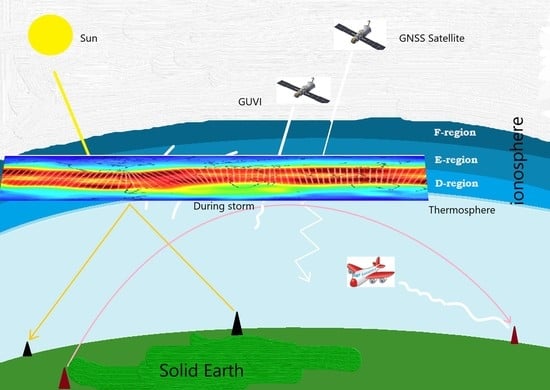
2. Materials and Methods

In this paper, we study ionospheric responses to the geomagnetic storms of 2015, 2018 and 2021 on global scale to find the sources that triggered the ionospheric variations. In particular, we analyze the 3-hourly geomagnetic Kp index, 1 min averaged electric Ey field, IMF Bz component, solar wind velocity Vsw, aurora AE index, geomagnetic disturbance storm time index (Dst), and solar flux F10.7 index. The data are available on the Omni Web of NASA at http://omniweb.gsfc.nasa.gov/ (accessed on 3 November 2022). The beginning of a geomagnetic storm usually exhibits a rapid decrease in the Dst index. The AE index can be used to study the energy transmitted to the auroral ionosphere during a storm. The Kp index can provide a good description of the storm’s magnitude; the Kp range is between 0 and 9. The PPEF data was obtained from the Cooperative Institute for Research in Environmental Sciences at https://geomag.colorado.edu/real-time-model-of-the-ionospheric-electric-fields.html (accessed on 3 November 2022).
The Global Ultraviolet Imager (GUVI) onboard the Thermosphere–Ionosphere–Mesosphere Energetics and Dynamics (TIMED) satellite senses far-ultraviolet emissions and provides thermospheric [∑O/N2] ratio maps [31]. These maps are obtained from https://guvitimed.jhuapl.edu/ (accessed on 3 November 2022). The [∑O/N2] ratio measures the electron density at the ionospheric F region; increases in N2 decrease electron density [32]. The thermosphere is the layer of the Earth’s atmosphere above the mesosphere that is distinguished by a low density of gas molecules and high temperatures caused by the absorption of intense solar radiation. It is mostly made up of atomic oxygen and nitrogen, with a trace of helium as well [10,13].
The TEC data from 15 different GNSS stations at low-mid and high-latitude regions were retrieved from the IONOLAB website, https://www.ionolab.org/ (accessed on 3 November 2022). Figure 1 shows the location of the GNSS stations used in this study, and Table 1 includes all detail. Slant TEC (STEC) is estimated as the number of free electrons in a square meter section along the line of sight between a GNSS satellite and receiver. The STEC units are TEC units (TECU), where 1 TECU = 1016 electron/m2. The STEC is obtained from IONOLAB and processed by the equations below [33].
S T E C = f 1 2 f 2 2 40.28 f 1 2 f 2 2 L 1 L 2 + λ 1 N 1 + b 1 λ 2 N 2 + b 2 + ϵ
S T E C = f 1 2 f 2 2 40.28 f 1 2 f 2 2 P 1 P 2 d 1 d 2 + ϵ
In this equation, carrier phase frequencies are presented by f1 and f2, pseudo-range is denoted as L, the delay path of the signal of carrier phase observations is P, the signal wavelength is λ, and the ray path uncertainty is N. Here, d and b denote the biases of consequent signal pseudo-range and instrumental carrier phase, and ϵ is the random error in the signal. The STEC is converted to vTEC using the following equation [34]:
v T E C = S T E C × c o s a r c s i n e R s i n Z R + H
In this equation, Z is the elevation angle of the satellite, and R and H are the Earth’s radius and the ionosphere height, respectively [35].
We also study the ionospheric indices from Swarm satellites to provide more evidence of vTEC variations from GNSS. The Swarm mission comprises three identical satellites, where Swarm A and C orbit at 440–460 km height and Swarm B track at 520–530 km height. These satellites carry sophisticated magnetometers, an electric field instrument to measure electron density (Ne), and a GNSS receiver to provide vTEC. All satellites have polar orbits with an inclination angle of 87°–88°. The vTEC data from Swarm are available at https://vires.services (accessed on 3 November 2022). The Swarm data were also analyzed during the different phases of the selected storms.
vTEC and dTEC from GNSS of the IGS network are analyzed in bi-hourly temporal resolution and spatial resolution of 2.5° by 5° in latitude and longitude, respectively [36,37]. The maps are available in the IONEX (IONosphere map Exchange) format at the Crustal Dynamics Data Information System (CDDIS) Goddard Space Flight Center (GSFC) of National Aeronautics and Space Administration (NASA) https://cddis.nasa.gov/index.html (accessed on 3 November 2022).
The new empirical vTEC model is used as quiet-time background to investigate the abrupt TEC anomalies during geomagnetic storms [38]. In this model, the principal component analysis reduced vTEC observables from 2003 to 2018 to a lower dimension. The resulting time-expansion coefficients were parameterized in terms of solar and magnetospheric forcing, annual, and LST cycles. The quiet magnetospheric forcing is set during the geomagnetic index condition at Am = 6. This scheme eliminates the diurnal, annual, and solar cycle variations. The residuals mainly show short-term variations due to magnetospheric forcing; i.e., those variations are mainly due to geomagnetic storms. The model is available at https://zenodo.org/record/3563463 (accessed on 23 November 2022).
The Earth’s magnetic field components are obtained from the magnetometer stations near the magnetic equator. These data help us to investigate the E region response during various phases of geomagnetic storms. The data at 1-min resolution are available at the INTERMAGNET network http://intermagnet.org (accessed on 13 November 2022). We employ data from the stations at HUA (America), GUA (Pacific Ocean), and MBO (Africa). The geographic and geomagnetic coordinates of the magnetometer stations are listed in Table 2, and their locations are shown in Figure 1. According to Biot and Savart’s law, ground magnetic field perturbations can be an integral part of ionospheric and magnetospheric electric current [39,40]. The horizontal component (H) of geomagnetic field can be computed using the north (X) and east (Y) components of the magnetic field (i.e.,  H = X 2 + Y 2 ). The observed H component corresponds to the current flow into the magnetosphere–ionosphere systems [41]. The equation is as follows:
H = SR + D
In this equation, SR and D represent the solar regular variations of Earth’s magnetic field due to regular ionospheric dynamo and the combined effect of various current systems flowing in the Magnetosphere Ionosphere system [42]. According to Le and Amoray-Mazaudier [40], the H component can be rewritten as follows:
H = H0 + SR + DM + Diono
In this equation, H0 and SR are Earth’s core induced baseline magnetic field and regular variation of Earth’s magnetic field on a given day, respectively. Magnetic field variations associated with the magnetosphere and ionosphere currents are represented as DM and Diono, respectively. The Diono is estimated as follows [40]:
Diono = H − DM − Sq; Diono = DP2 + Ddyn
In this equation, Diono consists of the combined effect caused by ionospheric disturbance due to polar currents (DP2) and dynamo currents (Ddyn) at low latitudes, DP2 is associated with PPEF, and Ddyn is associated with DDEF [40,43]. DM is calculated using the SYM-H index and the dip angle Φ as follows:
DM = SYM-H × Cos(Φ)
In Equation (6), Sq represents the selective quiet days (SR) average. Here, five quiet days are considered for computing Sq. We average the H component as suggested by the German Research Center of Geosciences (GFZ) (ftp://ftp.gfz-potsdam.de/pub/home/obs/kp-ap/quietdst/ (accessed on 3 November 2022)). The results are shown in Table 3, and the equation of Sq is as follows:
S q = H q u i e t = 1 n i = 1 n H i q u i e t
The EEJ at each station is computed by differences in the H component inside and outside the EEJ region at similar longitudes. These differences are related to the contribution of the EEJ current [44]:
EEJ = H1 − H2
In Equation (9), H1 and H2 are the averages of H components inside and outside the EEJ region, respectively.

3. Results

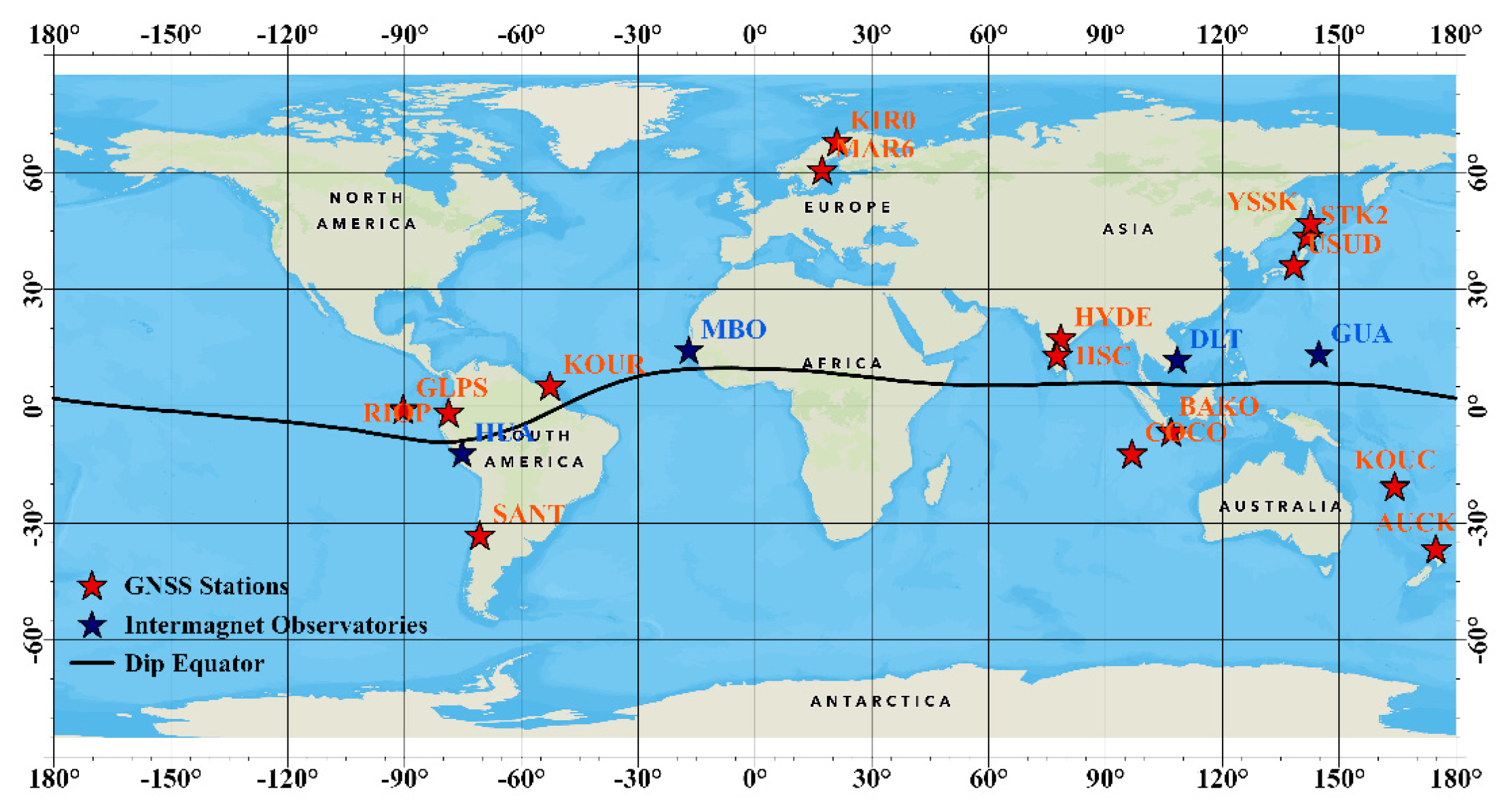
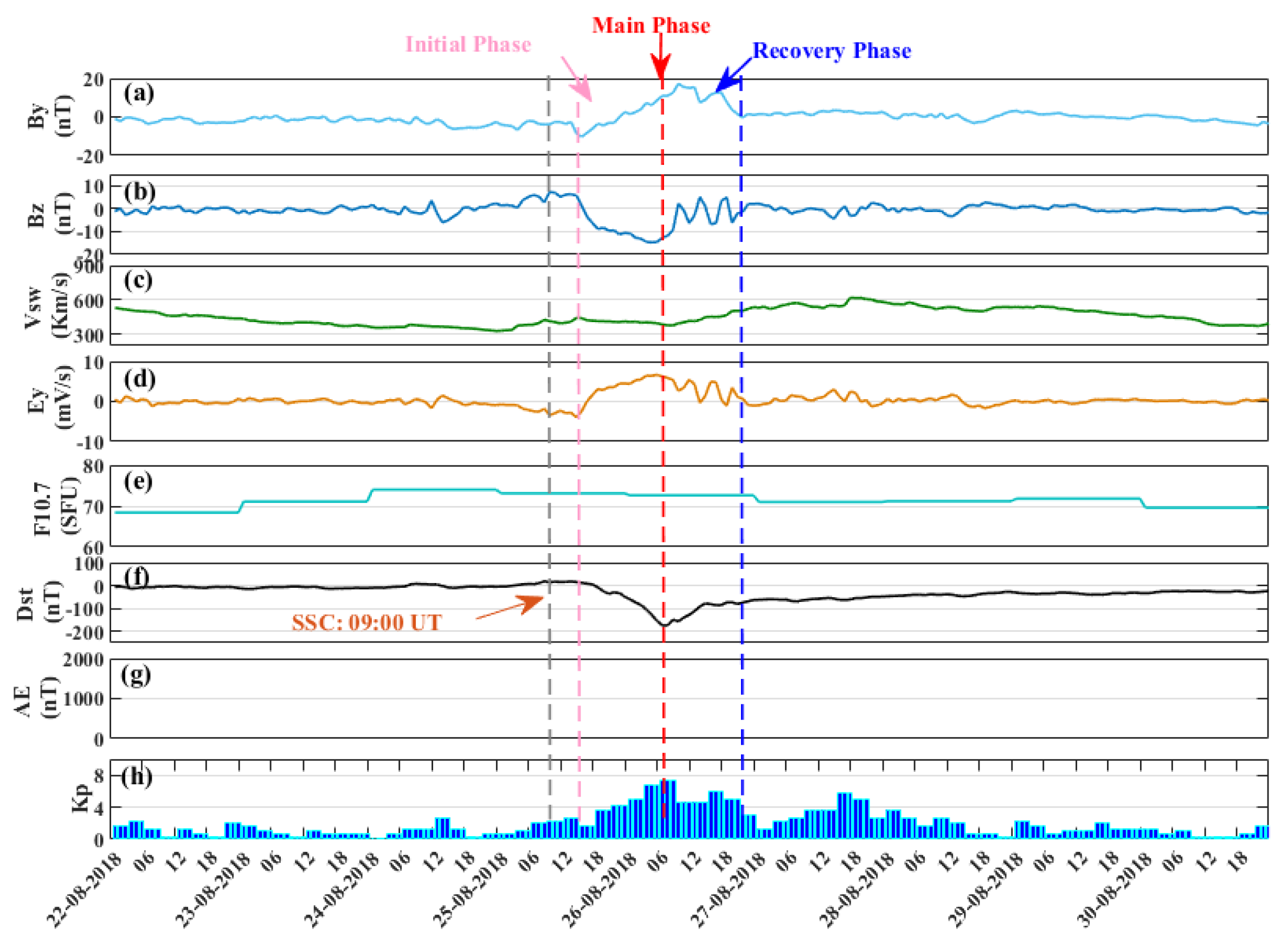
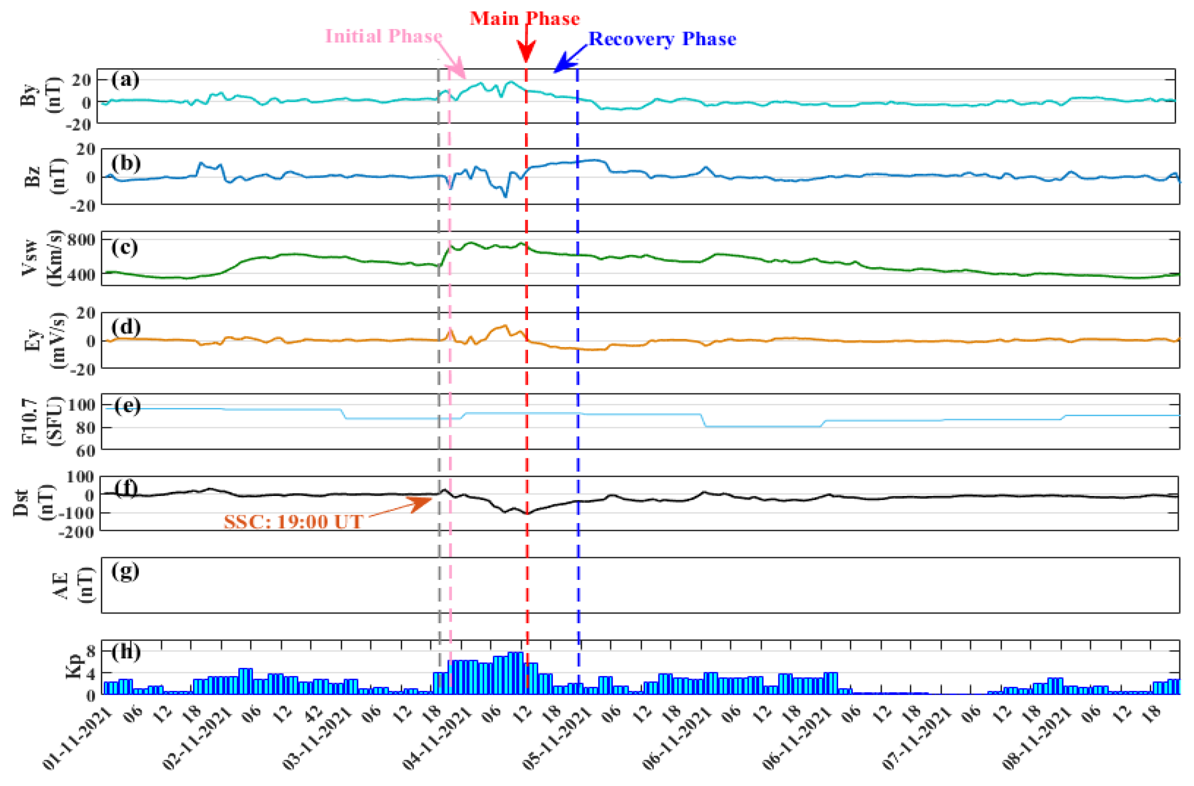
3.1. Geomagnetic Conditions of Storms in June 2015, August 2018 and November 2021

The geomagnetic storm of June 2015 occurred during solar cycle 24, and it was the second-largest known storm after the St. Patrick’s storm. On 22 June 2015, two CMEs hit the Earth’s magnetosphere at 05:45 UT and 18:35 UT. Figure 2 shows the sudden storm commencement (SSC), where the different phases are classified on the basis of different storm indices. The IMF Bz component shows a sharp southward turning immediately after the SSC, followed by a second southward IMF Bz before the main phase. IMF By exhibited the maximum positive peak of 20 nT just after the initial phase. These IMF By and Bz turnings are associated with more than 720 km/s speed of solar wind after the second SSC.
The storm of August 2018 occurred due to a large CME on 20 August 2018 (Figure 3). Later, a severe geomagnetic storm evolved as long-term southward IMF Bz, i.e., from 15:55 h UT on 25 August to 09:45 h UT on 26 August, thus allowing many particles to enter the Earth’s magnetosphere. IMF By showed a continuous rise towards the main phase of the storm. The SSC initiated at 09:00 UT on 25 August 2018. After 3 h of the SSC, at 09:00 h UT, a rapid drop in the Dst index was observed until 23:00 h UT on 23 August. The lowest Dst value was −203 nT around 07:00 h UT on 26 August.
The storm of November 2021 is due to CME associated with an M-class solar flare that left the Sun on 2 November (Figure 4). The shockwave that arrived on 3 November registered the strong geomagnetic storm as the Kp reached a maximum of eight, creating disturbances in Earth’s magnetic field. The IMF Bz component exhibited oscillation prior to the main phase with Dst < −105 nT on 13UT of 4 November. The IMF By component showed a significant positive peak of 18.1 nT accompanied by a solar wind of speed 760 km/s.

3.2. Ionospheric–Thermospheric Irregularities

During the three geomagnetic storms, the vTEC variations occurred at low-latitude stations in South America, South Asia, Southeast Asia, and the Oceania region (Figure 5 and Figure 6). During the initial phases of both the storms of 2015 and 2018, no clear enhancements in vTEC occurred at the low-latitude GNSS stations. On the contrary, COCO and BAKO stations exhibited peak vTEC variations during the initial phase of the November 2021 storm. However, the GNSS stations in Southeast Asia showed significant vTEC variations during the main phase for the storms 2015 and 2018. For the South American stations, only the KOUR showed significant variability. Although both storms were of similar intensity, vTEC enhancements of >50 TECU, 42 TECU < vTEC< 50 TECU, and 40 TECU < vTEC < 45 TECU occurred at the low-latitude stations of Southeast Asia, South Asia, and America, respectively, during the main phase of the June 2015 storm. On the other hand, vTEC variations occurred in the range of 18 TECU < vTEC < 20 TECU, 42 TECU < vTEC < 50 TECU, 40 TECU < vTEC < 45 TECU, and 18 TECU < vTEC < 20 TECU for the COCO, BAKO, South Asia, and KOUR GNSS stations during the main phase of the storm in 2018, respectively. There were no significant variations in vTEC during the recovery phases of the 2015 and 2018 storms, only a minor depletion at the South American stations. During the recovery phase, TEC depletions at the South American stations were more prominent in 2015 than in 2018. Furthermore, the mid-latitude stations of Southeast Asia and Asia exhibited significant vTEC variations of >50 TECU during the initial phase of the 2021 storm, and South American stations exhibited prominent variations vTEC during the main and recovery phases (KOUC, GLPS and RIOP exhibited enhancement of >58 TECU, 55 TECU and 56 TECU, respectively in Figure 6).
The vTEC variations at the mid-latitude GNSS stations are shown in Figure 7 (2015 and 2018 storms) and Figure 8 (2021 storm). We analyze the AUCK station in New Zealand, the STK2 and USSD stations in East Asia, the YSSK station in Russia, and the SANT station in Chile. During the initial phases of both storms of 2015 and 2018, no clear vTEC variations occurred in any of the stations, except the SANT station, which exhibited significant variation in the 2015 storm. On the contrary, all stations exhibited fluctuations during the initial phase of the 2021 storm (Figure 8). Furthermore, all stations except SANT exhibited enhancement in vTEC followed by a sharp decrease and then rise in vTEC in the main phase of the 2021 storm (AUCK vTEC to 28 TECU followed by a drop of 5 TECU, STK2 vTEC enhanced to 23 TECU followed by a drop of 8 TECU, both USUD and YSSK vTEC rose to 30 TECU followed by a drop of 14 TECU). The mid-latitude stations showed significant peaks in vTEC in the initial phase of the 2021 storm. During the main phases of the 2015 and 2018 storms, sharp enhancements are observed at all stations except the SANT station. The vTEC during the main phase of the 2015 geomagnetic storm in Oceania, East Asia, and Russia is 30 < TECU < 40, 30 < TECU < 40, 20 < TECU < 30, respectively. On the other hand, Oceania, East Asia, and Russia exhibited 10 < TECU < 20, 10 < TECU < 20, 10 < TECU < 20 during the 2018 geomagnetic storm, respectively. None of the mid-latitude stations showed significant anomalies during the recovery phases of all three storms.
The vTEC at the high-latitude stations of KIR0 and MAR6 in Sweden and Europe is shown in Figure 9 (2015 and 2018 storm) and Figure 10 (2021 storm). In this figure, enhancements of 2 TECU in KIR0 are shown within 2 h after the SSC of the storm of 2015. Then, a sudden depletion until the main phase of the storm occurred. Similarly, the MAR6 station increased 4 TECU after the SSC, and then a depletion in the main phase occurred. In the recovery phase, no increases were seen for either station. In the storm of 2021, minor fluctuations in vTEC during the initial phase were observed. However, MAR6 and KIR0 showed peak vTEC values of 19 TECU and 18 TECU during the recovery phase of the 2021 storm.
The TEC variations in GIMs for the storms of 2015 and 2018 are shown in Figure 11 and Figure 12. During the storm of 2015, all three American, African, and Asian sectors showed a moderate high-latitude enhancement after the SCC at the southern latitudes. Then, the American and African sectors showed significant enhancement at the low-latitude regions above 15 TECU, whereas the Asian sector showed depletion of similar magnitude. For this storm, the high-latitude regions showed a clear depletion during the main phase for all the three longitudes. During the main phase of the 2018 storm, vTEC enhancement is very prominent in the American and African sectors compared to the Asian sector. Compared to the storm of 2015, no clear depletions were seen at any location.
Figure 13 shows the ∑O/N2 ratio during the storms of 2015 and 2018. The African sector showed reductions in the initial phase and enhancement in the final phase at low and mid-latitudes of the 2018 storm. This resulted in the increment of vTEC in the African region, whereas we observed an enhancement in the ∑O/N2 ratio after the main phase of the 2015 geomagnetic storm coinciding with the vTEC increment in the African sector. The Asian, Australian, and Oceania regions also showed significant enhancements in the ∑O/N2 ratio during the main phase of the 2018 geomagnetic storm, and no such enhancement/depletion was visible for the 2015 geomagnetic storm during the main phase. This resulted in a significant increase in vTEC in the abovementioned regions during the main phase of both storms. On the other hand, we also observed an enhancement in the ∑O/N2 ratio in South America during the initial phase of the 2015 storm and the recovery phase of the 2018 geomagnetic storm. There have been several reports on enhancement/depletion in ∑O/N2 ratio (reduction/enrichment in vTEC) in different parts of the world through thermospheric ∑O/N2 variability [3,10,12,13,16,23,44,45].
vTEC data from Swarm satellites for the 2015 and 2018 storms are shown in Figure 14 and Figure 15. Clear enhancements in vTEC were seen in the American region at the low and mid-latitudes during the initial phase of both storms; no clear variations were observed for the Asian region during the initial phase of either storm. The low and mid-latitudes of the Asian and African regions depicted larger vTEC variations than those in the American sector during the main phase of both storms. During the recovery phase of both storms, larger variations were observed in the American region than in the Asian sector. The vTEC values from Swarm during the main and recovery phases were different than those from the GNSS stations in Asia, Australia and Russia.
The PPEF variations at low-and mid-latitude regions during 2015 and 2018 storms are shown in Figure 16. Similarly, Figure 17 shows the PPEF variation of the 2021 storm. The PPEF variations during the 2018 storm were smaller than those during the storm of 2015. This differs from the results obtained through GIMs (Figure 11 and Figure 12). The storm of 2021 exhibited more prominent PPEF variations than the 2018 storm. More intense PPEF was observed during the initial phase compared to the main phase and recovery phase of the 2021 storm. This strong PPEF occurred in between 0°–60° in the east side and −60° to −120° in the west side in the initial phase. However, peak PPEF was observed 3 h prior to the main phase in the west region from −60° to −180°. Moreover, strong PPEF occurred at all longitudes during the main phase of the storm of 2015, while the PPEF peak during the 2018 storm occurred in the Far East and West. During the main phase of both storms, stronger PPEF occurred compared to that seen during the other phases.

3.3. Earth’s Magnetic Field Variations

The variations in the Earth’s magnetic field during the storms of June 2015 and August 2018 are shown in Figure 18. Figure 19 shows the November 2021 storm-induced variations in Earth’s magnetic field. We investigate the variations in the H component of Earth’s magnetic field, and the EEJ estimated from INTERMAGNET stations near the magnetic equator. It shows significant variations in the SSC events during all three storms of 2015, 2018 and 2021, followed by a considerable decrease in Earth’s horizontal component during the recovery phases. However, the lowest negative peak of −105 nT was exhibited on 4 November 2021 at 14 h UT, whereas the largest disturbances of the H component in the American region (HUA station) reached 259.92 nT on 22 June 2015 at 20:49 h UT. On 25 August 2018 at 23:55 h UT, the initial phase of the storm reached −123.91 nT. The Dion exhibited a decrease in the initial phase, followed by an increase in the main phase, due to H minima during nighttime in the South American region. Two negative peaks in the H component were observed during the storm of June 2015 in the Pacific region, one during the beginning of the initial phase and the other during the main phase. Similarly, only one negative peak was observed in the main phase during the storm of August 2018. However, both the Pacific Ocean and Asia region exhibited two negative peaks, where one was during the initial phase and other one coincided with the main phase. The values of Dion exhibited abrupt variations for all three storms after each SSC, corresponding with the variations in the H component. The MBO station in Africa and the DLT station in Asia showed prominent decreases in the H component for both storms of 2015 and 2018, respectively. The lowest values were −207.12 nT for the storm of June 2015 and −107.78 nT for the storm of August 2018. The vTEC variations triggered by Dion were prominent at different longitudes, specifically during the SSC and the main phase of the storm of June 2015. No clear variations were seen at the HUA station during the storm of August 2018. On the contrary, vTEC variations triggered by Dion were more prominent in the initial and main phases of the November 2021 storm at different longitudes.

4. Discussion

The vTEC enhancements during the storms of June 2015, August 2018 and November 2021 were initiated approximately 4–6 h after the SSC events at the low-latitude regions in East Asia, Southeast Asia and Oceania. All the three sources of vTEC data used in this study, i.e., GNSS, Swarm, and IGS GIM TEC, provided similar results with minor differences, specifically between GNSS and IGS GIM TEC, most likely due to local anomalies not well represented by GIM TEC [45,46,47]. All the vTEC enhancements occurred during the main phase for all three datasets. The variations at different geographical coordinates followed the PPEF and thermospheric ∑O/N2 variations. Moreover, the PPEF enhancements started at the SCC in Asia and Oceania, along with the ∑O/N2 enhancements leading to clear effects during the main phase at the low-latitude regions (Figure 13 and Figure 16). East Asia, Southeast Asia and Oceania exhibited vTEC enhancement during the initial phase (Figure 6 and Figure 17). These positive enhancements are due to PPEF and the increment of oxygen [48]. No prominent enhancements or depletions occurred in the South American sector, most likely due to Dst minima, along with depletion in the recovery phase due to a drop in ∑O/N2 ratio (Figure 5 and Figure 13).
At the mid-latitudes, the Asia–Oceania region exhibited peak values during the main phase, coinciding with Dst minima for both the 2015 and 2018 storms. The station in South America exhibited depletions at the nightside during the storm of June 2015; the storm of August 2018 lacked this feature. However, all stations of November 2021 storm showed enhancement during the initial phase, followed by a drop and then another rise in vTEC, except the Chile region, which demonstrated a continuous increase in vTEC in all phases. The EIA expansion from equatorial to mid-latitude regions was responsible for vTEC enhancements at all longitudes. Both the storms of June 2015 and August 2018 revealed that Dion and ∑O/N2 drivers control these fluctuations. The PPEF and Diono were the main reasons behind these fluctuations in the November 2021 storm. In fact, Fuller-Rowell et al. [46], Mannucci et al. [7], and Vankadara et al. [49] presented similar results. The PPEF plays a vital role in vTEC enhancements through plasma diffusion along magnetic field lines, thus creating the fountain effect during the daytime [7]. The depletions seen in vTEC were due to variations in thermospheric composition, such as those generated by recombination processes creating N2. These depletions were observed in the recovery phase of both 2015 and 2018 storms in the low-latitude South American regions (Figure 5 and Figure 13).
The external electric field can penetrate the equator to disturb low and mid-latitudes, as they are connected to the inner magnetosphere through closed magnetic field lines. External sources should also be considered, taking into account the fundamental forces that drive the penetration of electric field, such as solar wind drivers. Nishida [43] compared the north–south oscillation in IMF with the geomagnetic fluctuations, and considered PPEF a temporary failure mechanism of shielding. PPEF can exhibit multiple pulses, as it is the direct consequence of IEF fluctuations [50,51]. Magnetic reconnection is an important parameter for dusk-ward PPEF processes (lasting < 3 h). The dawn-ward IEF shows the opposite behavior: as long IMF Bz oscillates between northward and southward polarity, dawn-ward IEF rarely does. The shielding effect would not fully develop under these circumstances and would not cancel the PPEF during the short pulse of dusk-ward IEF. Nevertheless, this is only sometimes the case, since the transition to the northward IMF Bz component does not necessarily generate over-shielding. However, the reduction in the convective electric field can transit to over-shielding status [52]. The magnetosphere under sustained pressure due to dense solar winds can suppress the development of electric field shielding during multiple PPEF events. PPEF can exhibit long-duration patterns if the magnetic activity is strengthened under storm conditions [53]. In this work, PPEF was demonstrated to generate variations in vTEC throughout the globe, except for the South America region, which was more prominent during the storm of June 2015. The max PPEF was confined to only the far east and west regions during the storm of August 2018, depicting clear variations in Oceania and not in the American sector. As the storm commenced, Asia, Oceania, and Russia exhibited vTEC enhancements at the low and mid-latitudes due to PPEF. Storm-time variations at the low and mid-latitudes were generated by a large fountain effect, creating a stronger EIA. Many researchers have reported these effects [25,30,54,55,56]. The ionosphere exhibited a variable response along different longitudes. This has been confirmed by different magnitudes of PPEF and satellite data (Figure 5, Figure 6, Figure 7, Figure 8, Figure 9, Figure 10, Figure 14, Figure 15, Figure 16 and Figure 17). The influence of PPEF in EIA shows significant longitudinal differences during geomagnetic storms.
As we know, ionospheric F-region density is controlled by photoionization, neutral winds, expansion and transportation due to EXB drift and ambipolar diffusion. It is well understood that ionospheric density is not reliant on any peculiar driver or single process. The expansion of EIA in the F region occurred due to the zonal electric field in general, and this process alone is not responsible for storm-time ionospheric variations. Additionally, the zonal variation in the electric field cannot form the ionospheric expansion itself in this study. The direct tidal impact cannot be due to the large-scale zonal electric field either, as the neutral tides develop tilted phase fronts due to vertical spread. Therefore, the ionospheric height occurred due to high and low thermospheric density at different longitudes and this will vary in height during storms. This can be a possible hypothesis of ionospheric expansion during storms, which needs more study and thus beyond the capacity of this paper. However, in this paper, we analyzed significant storm time vTEC variations mainly controlled by ∑O/N2, Dion and PPEF.
During these geomagnetic storms, the Earth’s magnetic field observations at different longitudes make it possible to comprehend the processes of large-scale ionosphere electric currents. There are two main types of disturbances, DP2 and Ddyn, which are associated with PPEF and DDEF, respectively. Ddyn exhibits a more dynamic variation than DP2, which lasts only 2 to 3 h [40,43]. During these geomagnetic storms, normal circulation of thermospheric winds is perturbed due to moment transfer and energy inputs at high latitudes, giving eastward and westward electric fields at the nightside and dayside, respectively [45,57]. Diono exhibited large nighttime enhancements at the low-latitude stations. These variations are associated with PRC, as indicated by ASYM-H (Figure 18a,a` and Figure 19a). The anti-Sq signatures observed during the recovery phase in the magnetic data are due to the orientation of electric fields [58]. Vankadara et al. [49] performed a similar study, showing Dion minima at different Local Solar Time (LST) locations, leading to equatorial plasma bubble developments. Our results have shown differences in longitude because of magnetospheric convection processes and electric field penetration [59]. In this scheme, all three American regions have shown clear variations in the initial phases of both the June 2015 and August 2018 storms, but none in the main phases of either storm (Figure 5, Figure 7, Figure 11, Figure 12, Figure 14 and Figure 15). However, the low-latitude region of America exhibited vTEC peaks in the recovery phase, and mid-latitude stations had fluctuations in the initial phase of the storm of November 2021 (Figure 6 and Figure 8). Asia, Oceania, and Russia showed vTEC enhancements during the main phases of the June 2015 and August 2018 storms (Figure 5, Figure 7, Figure 11, Figure 12, Figure 14 and Figure 15). Various authors have shown latitudinal and longitudinal ionosphere responses due to PPEF [60,61,62,63,64]. EEJ variations at different longitudes are due to the underlining effects of local winds, which are responsible for EEJ driving [65,66,67,68,69]. In addition, longitudinal differences in EEJ are caused by the different nature of the propagating diurnal tides, the meridional winds, and the dynamics of the migratory tides [70,71,72,73,74]. All the satellite and ground data showed significant storm-time variations in different phases [75,76,77,78,79]. These satellite data also showed variations in the lower ionosphere [80,81,82,83,84,85]. In this study, clear EEJ enhancement has been observed at the beginning of both the 2015 and 2018 storms. In the American region (Figure 18e), EEJ resulted in vTEC variability in the initial phase, but no clear variability along the main phase. In the Asian region, the EEJ increment was more prominent during the main phase (Figure 18e`), leading to vTEC enhancements in the low-latitude stations (Figure 5a–c,a′–c′). However, EEJ enhancement was more prominent in the American region during the November 2021 storm, leading to vTEC enhancement in all American regions (Figure 6e,f,h and Figure 8e). Our results demonstrate the existence of longitudinal variability due to EEJ during storm-time conditions. The dependence of EEJ strength can be explained by varying the cross-section area of the longitudinal Cowling channel. We analyzed the storm-time variations in the ionosphere during three different storms on a global scale using multiple ground and satellite data to comprehend their effect on multiple atmospheric layers. However, more satellite data with better temporal and spatial resolution are required for the forecasting of geomagnetic storms and their impacts on a global scale.

5. Conclusions

The upper-atmospheric responses to the 22–23 June 2015, 25–26 August 2018 and 3–4 November 2021 geomagnetic storms have been investigated for different regions of the world. The ionospheric variations during the storms are also shown in the context of different drivers at global and regional scales during the three storms. The main conclusions are as follows.
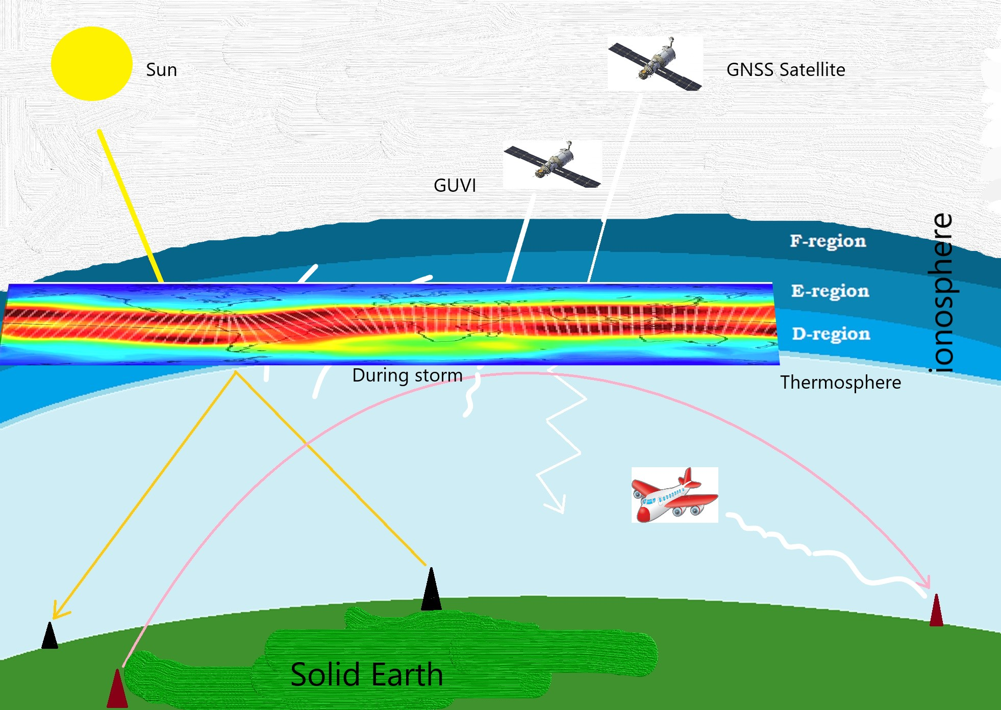
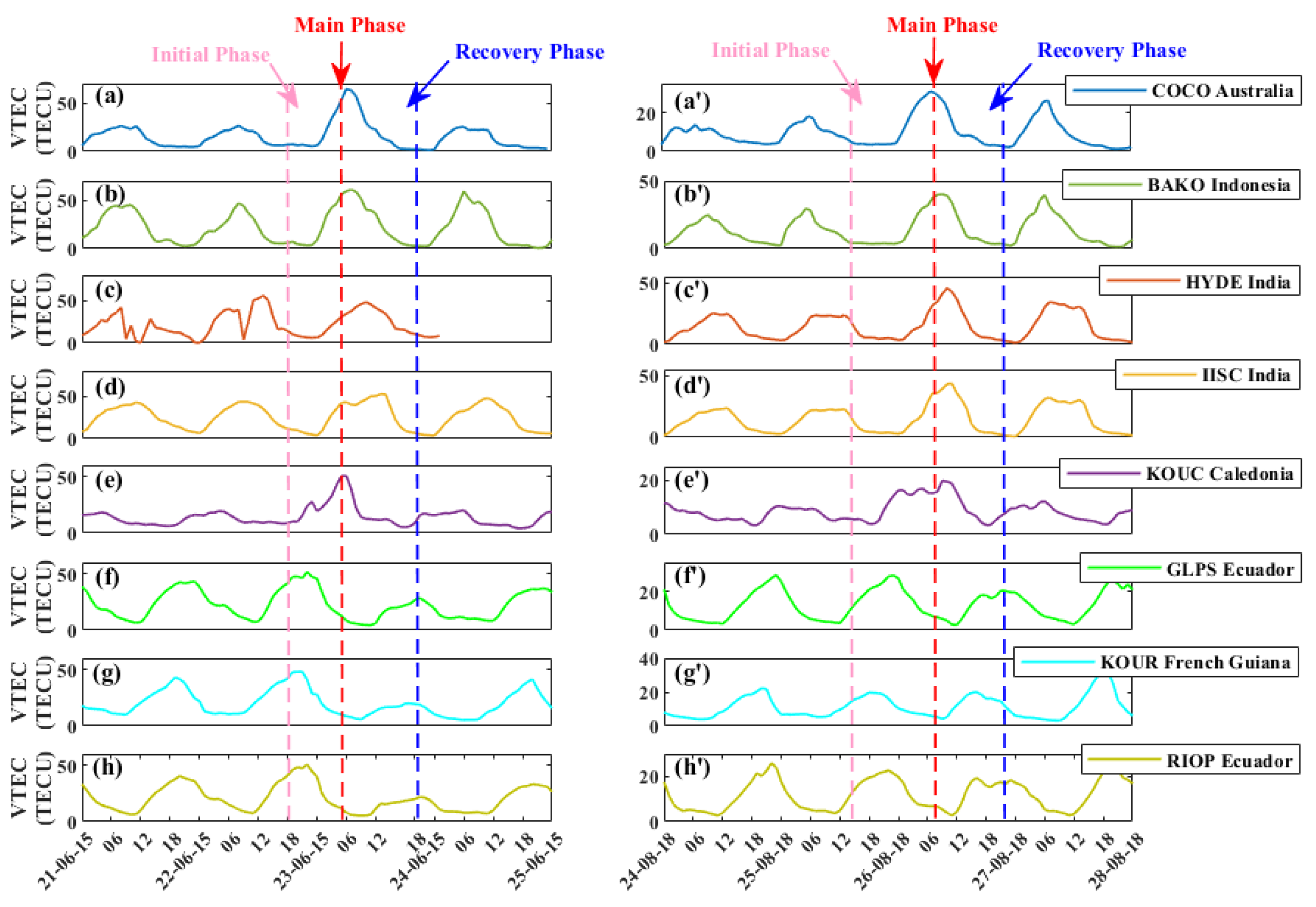
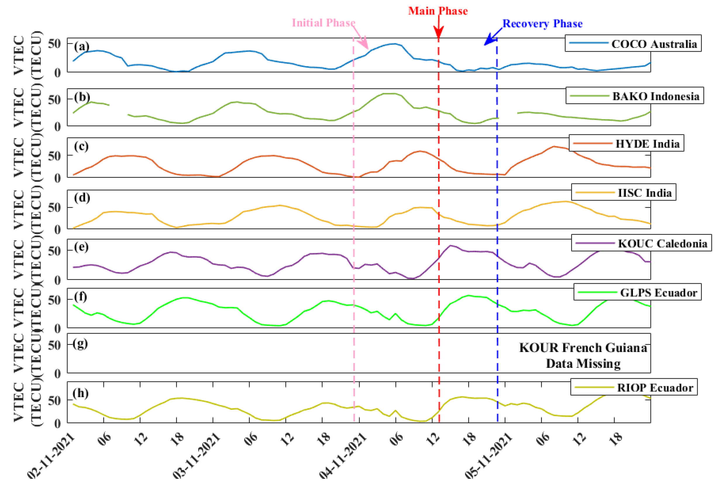
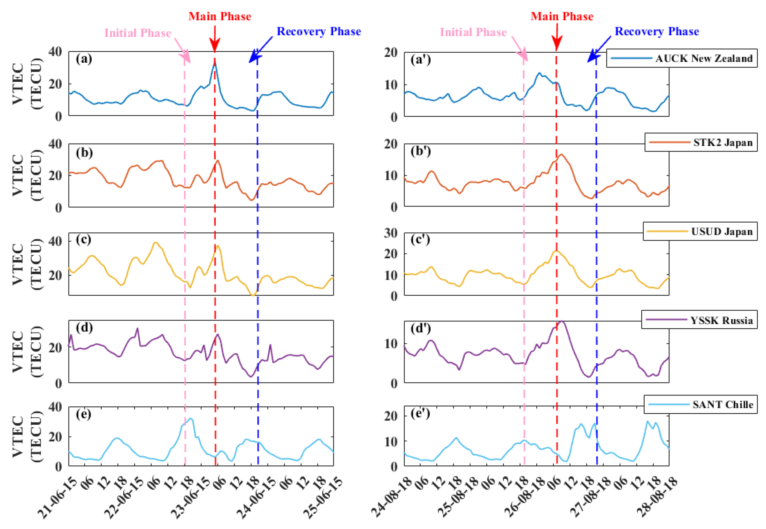
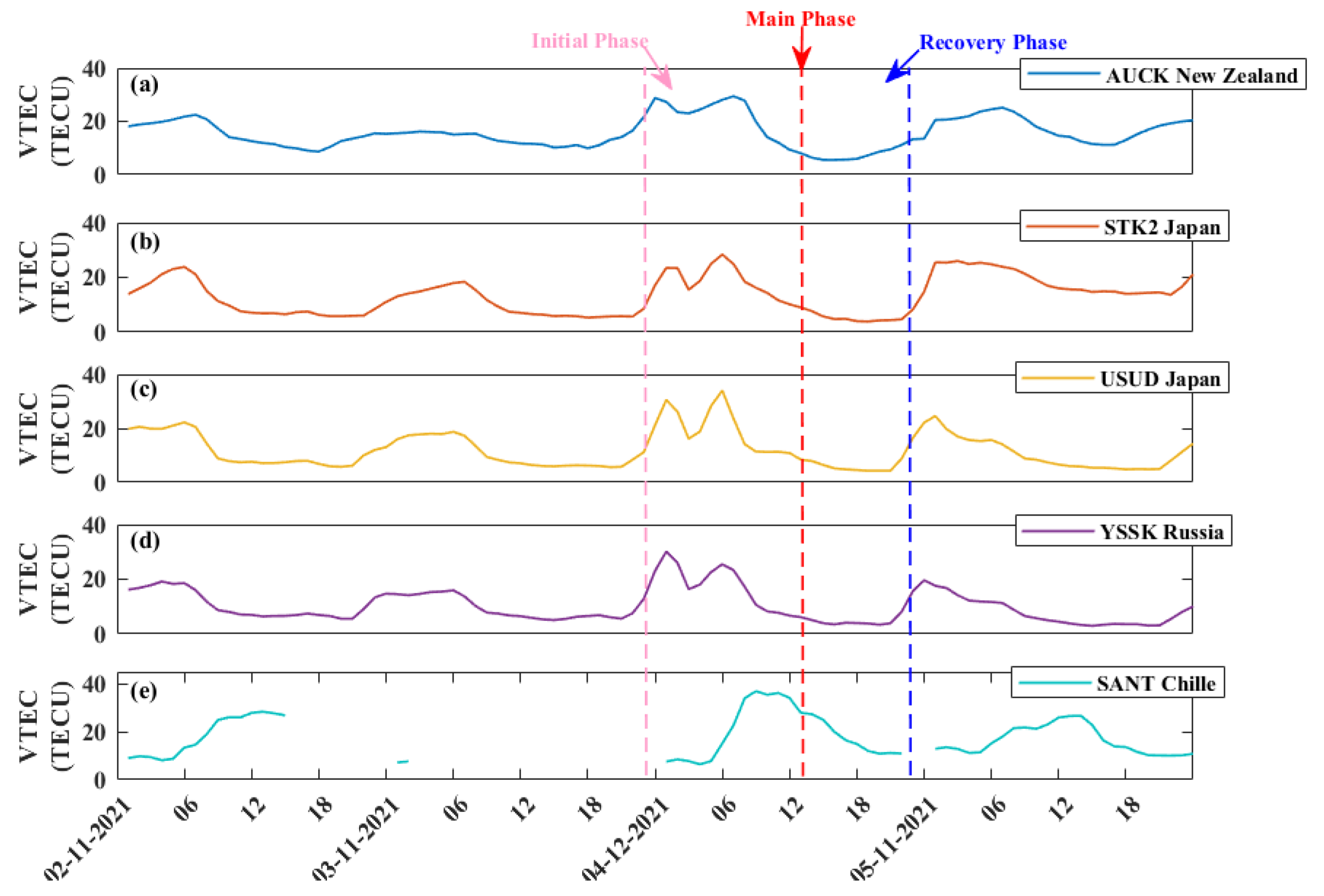
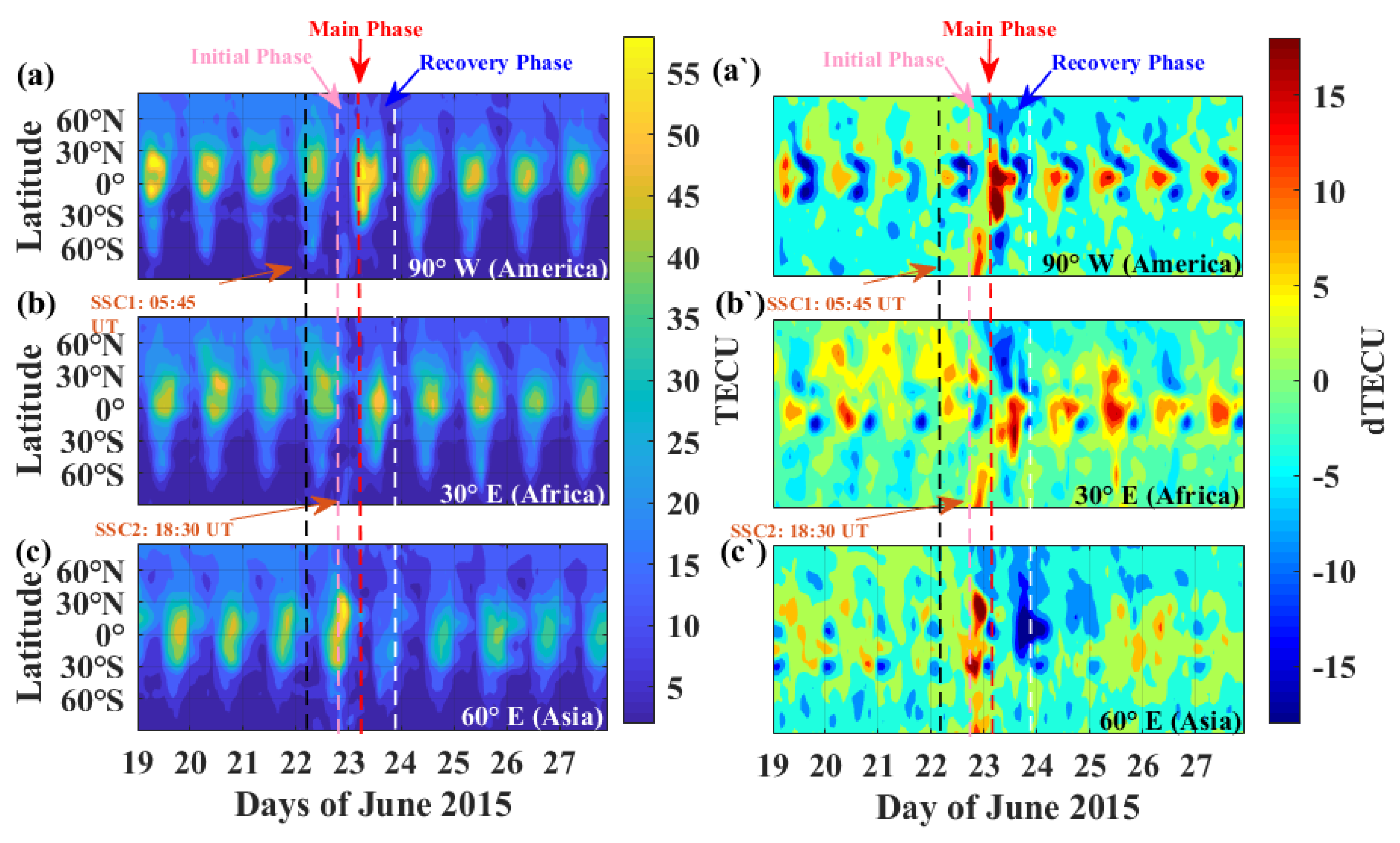
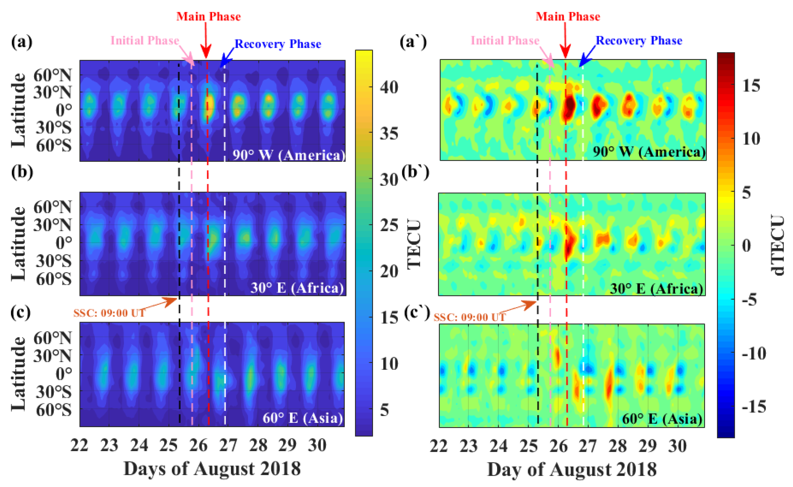
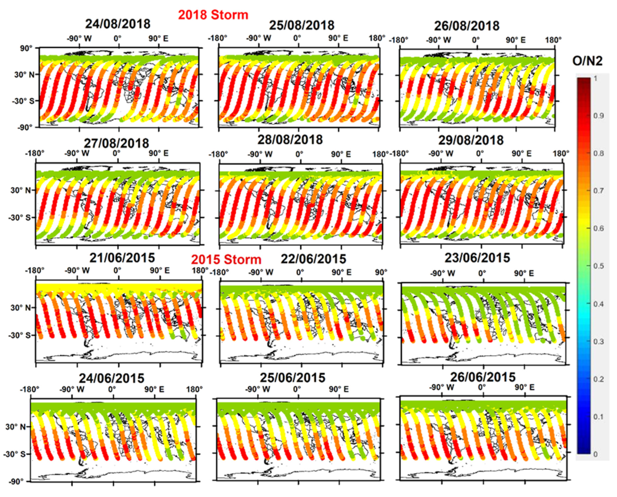
  • Different regions exhibited variable vTEC enhancement/depletion patterns depending on thermospheric ∑O/N2 ratio reduction/enrichment. At low latitudes, the GNSS stations of East Asia (HYDE and IISC), Southeast Asia (COCO and BAKO), and Oceania (KOUC) showed vTEC enhancement in the main phases of the storms of June 2015 and August 2018. The stations in South America (GLPS, KOUR and RIOP) registered no such enhancements. However, both East Asia and Southeast Asia region showed vTEC enhancement during the initial phase of the 2021 November storm. Similarly, GLPS and RIOP stations of South America showed enhancement in vTEC during the recovery phase of the 2021 storm. vTEC enhancement in the Asian and Oceania regions was approximately double the value during the quiet days for both June 2015 and August 2018 storms. The GNSS stations exhibited enhancement during all three storms at the mid-latitudes of Oceania, East Asia, and Russia. Oceania, East Asia and Russia exhibited enhancement during the initial phase of the November 2021 storms, followed by a sharp decrease and then a rise in vTEC.
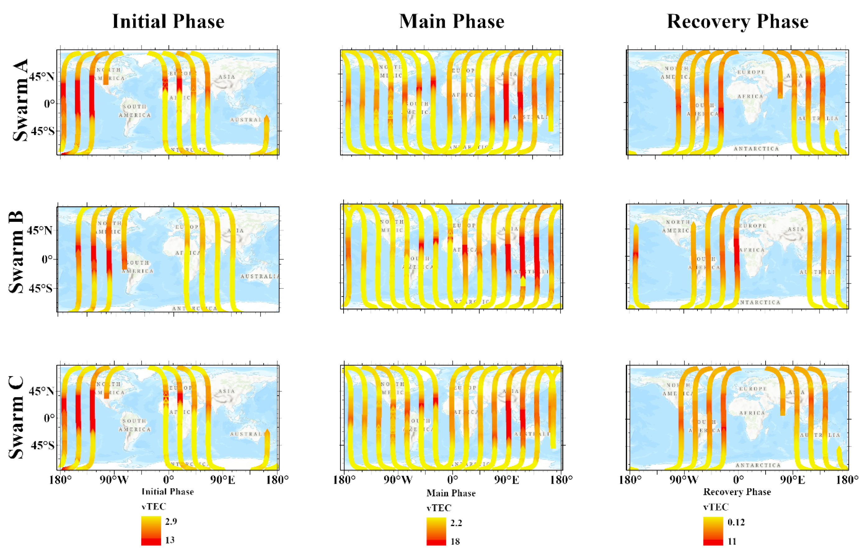
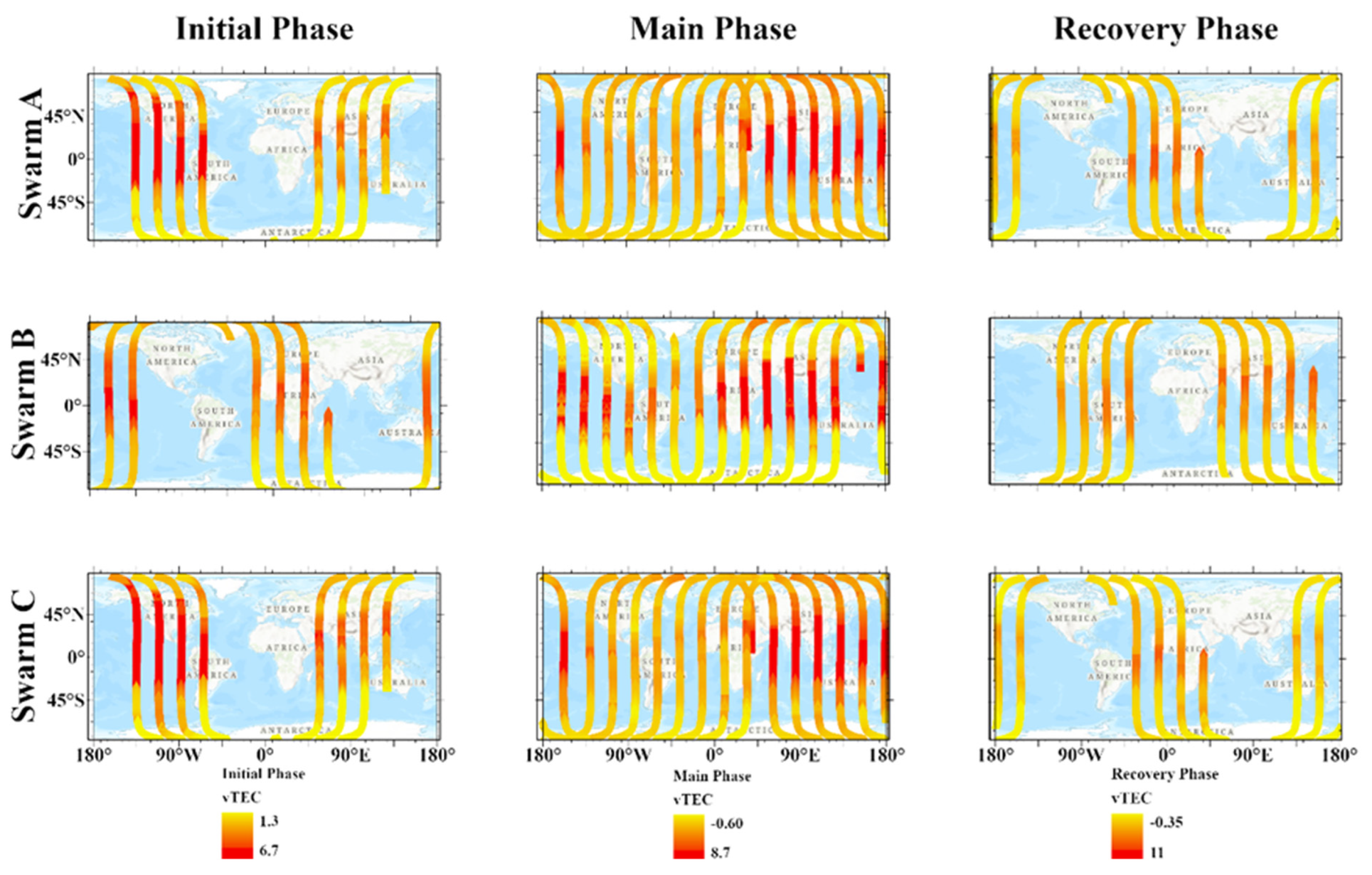
  • Swarm satellites vTEC confirmed the low-and mid-latitude ionospheric irregularities during the main phases of the storms of June 2015 and August 2018.
  • GIM-TEC also showed clear agreement with the GNSS-derived vTEC in most parts of the world during the main phase of both the June 2015 and August 2018 storms. During the main phases of both storms, these ionospheric variations at low-and mid-latitude regions were mainly driven by thermospheric ∑O/N2 ratio, PPEF and EEJ.
  • The PPEF variations at different longitudes provided different vTEC responses. These variations were present in the low-and mid-latitude regions of Asia, Africa, Russia, and Oceania for all three storms. The southward–northward oscillation of the IMF Bz component drives this variability along with interactions with Earth’s magnetosphere and solar wind. vTEC enhancement at different longitudes were mainly attributed to PPEF variability. vTEC depletion were mainly due to the enriched thermospheric wind composition, as seen by changes in the ∑O/N2 density ratio.
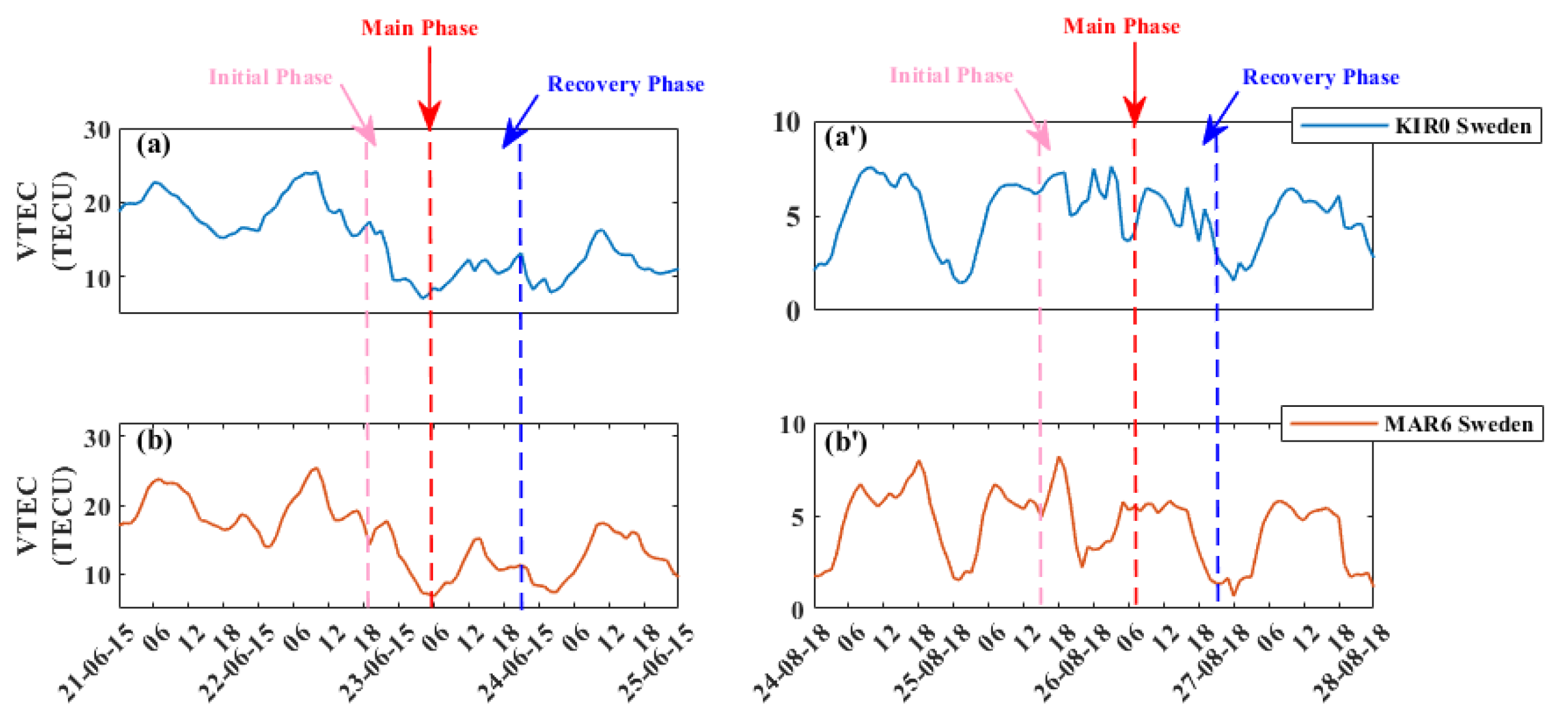
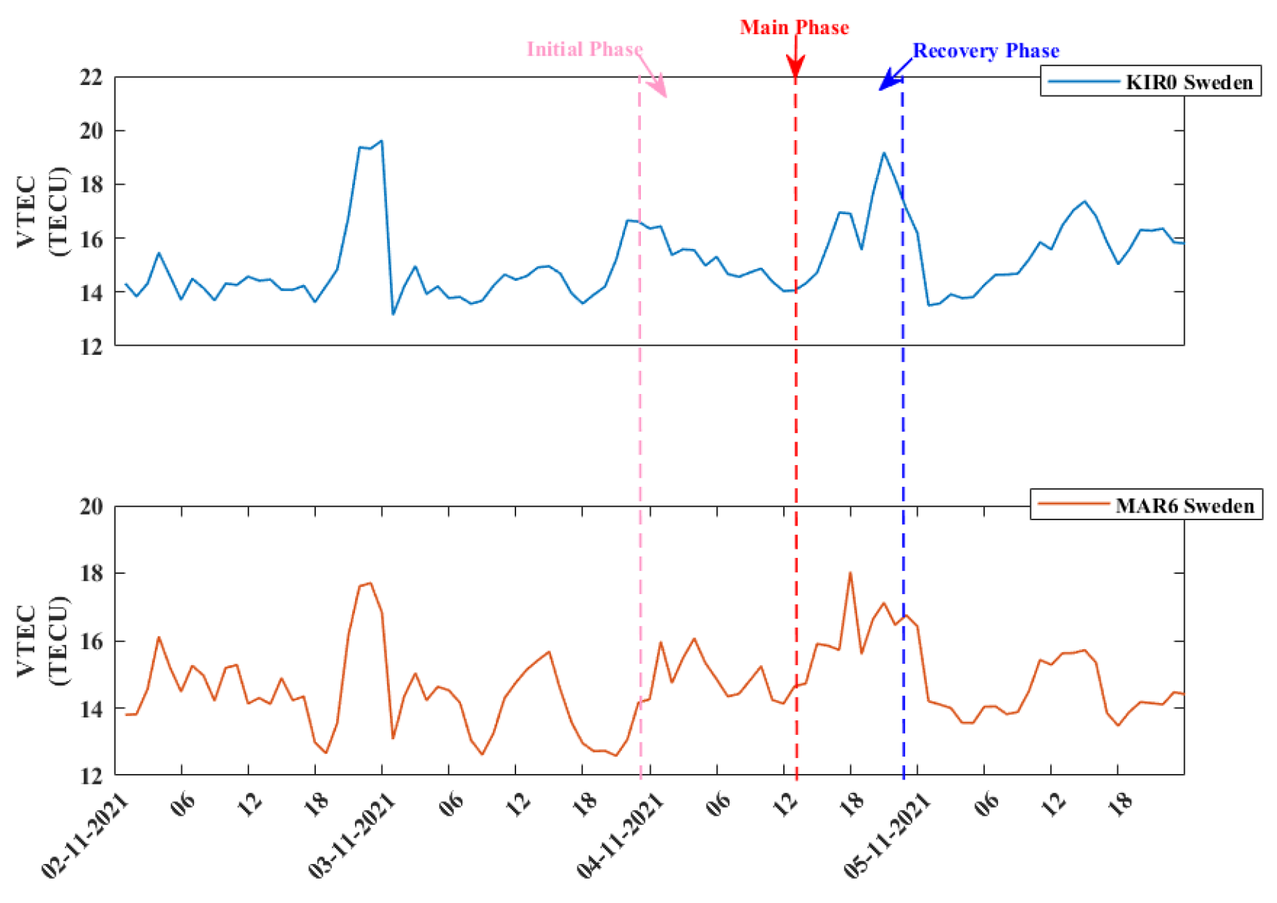
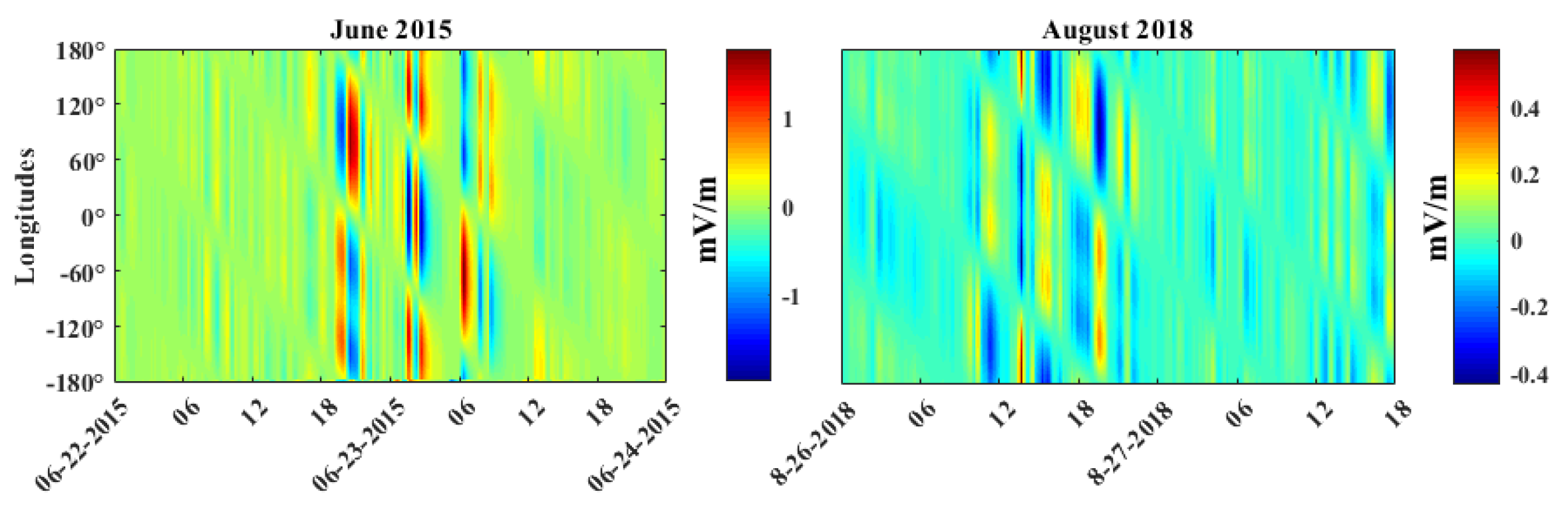
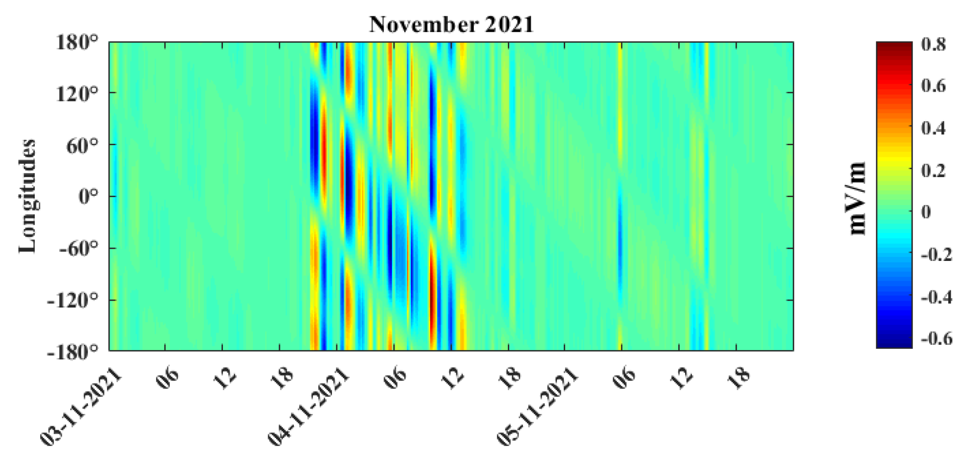
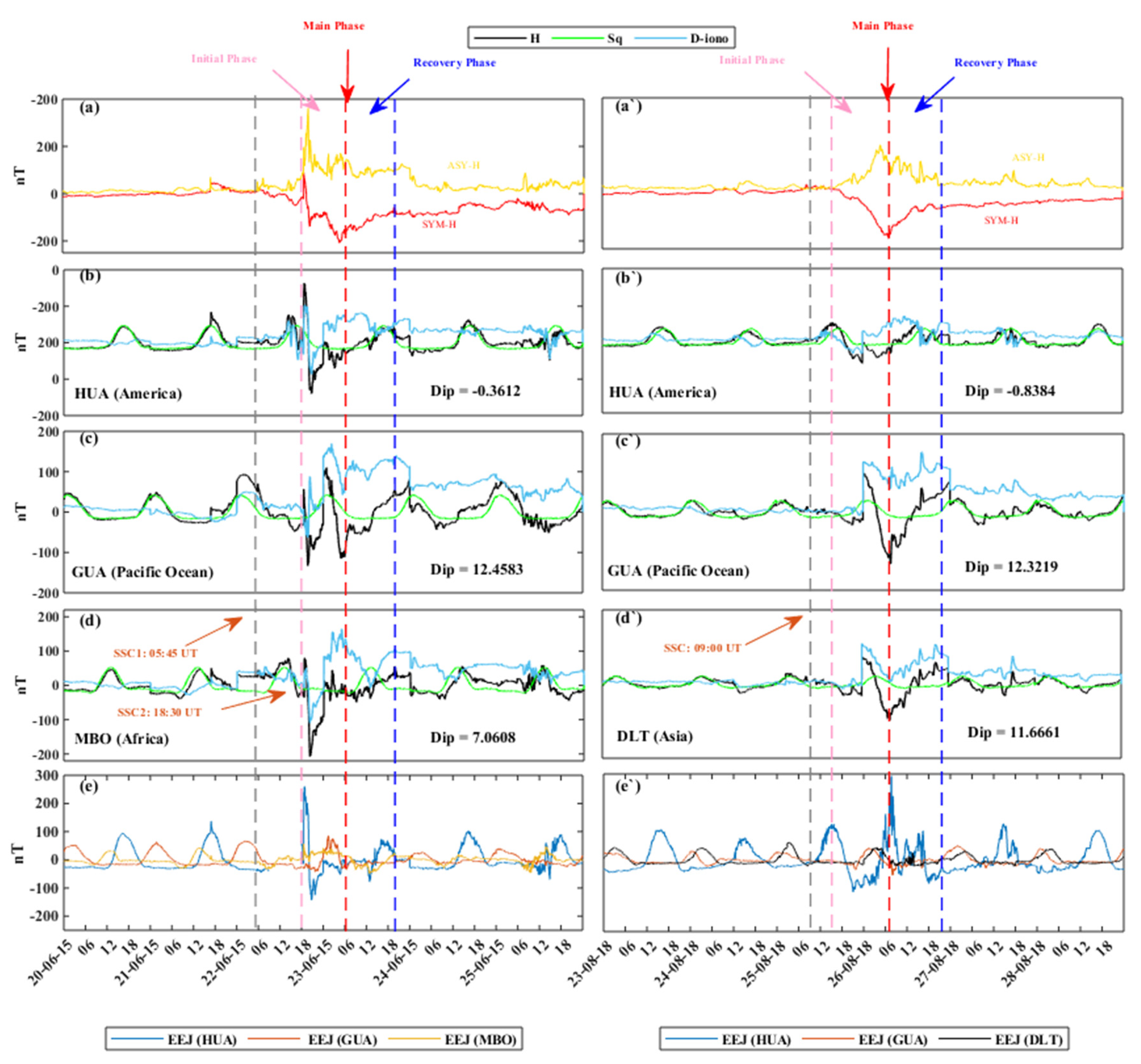
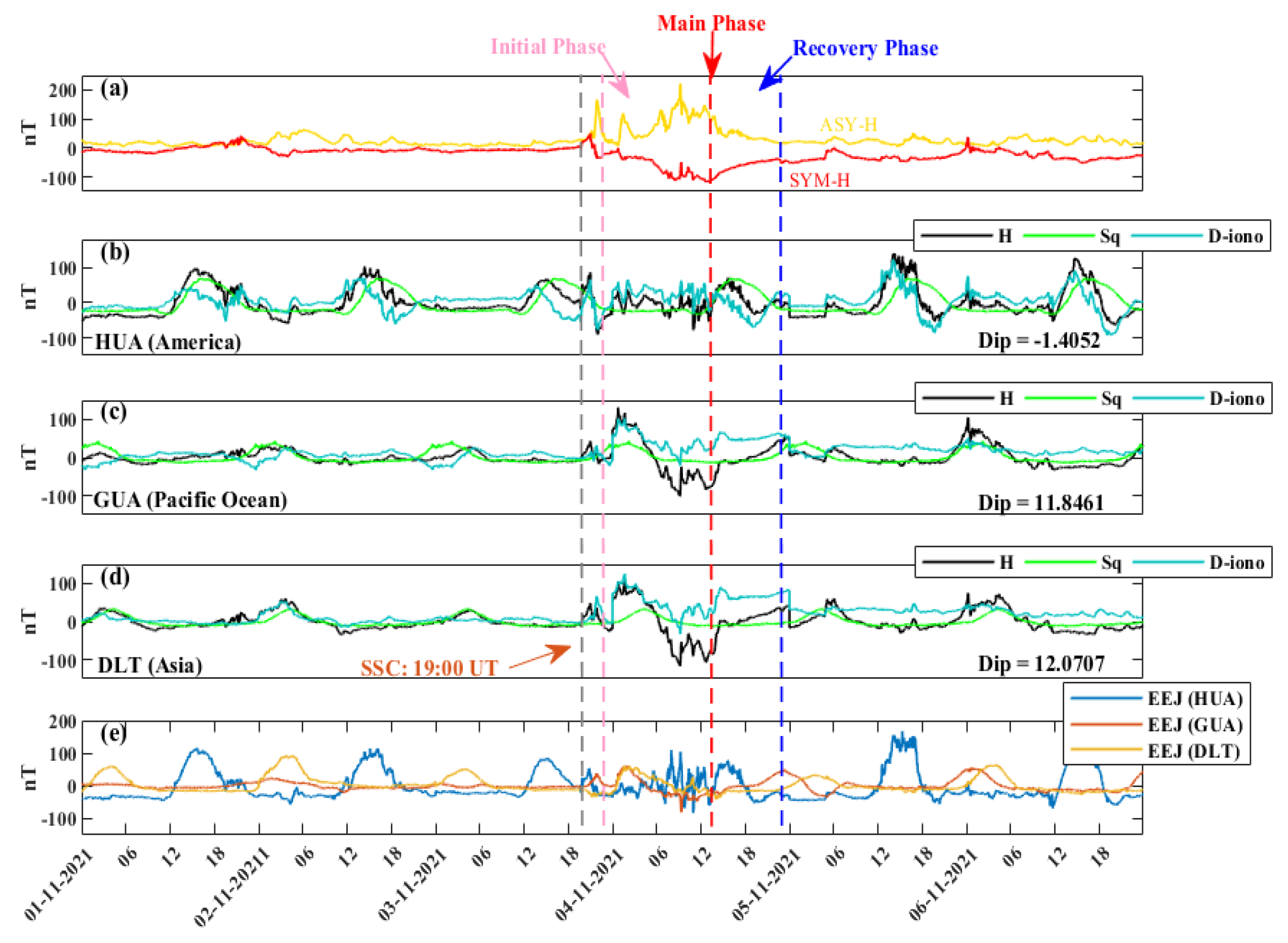
  • The Dion from the H component of the Earth’s magnetic field exhibited clear variations during the 2015 storm compared to the 2018 and 2021 storms.

Author Contributions

Conceptualization, M.S.; methodology, software, R.S., M.S., M.A.T. and A.C.; writing—review and editing, R.S., M.A.T., A.M.-M., P.J. and L.L. All authors have read and agreed to the published version of the manuscript.

Funding

This research is financially supported by National Natural Science Foundation of China (grant No. 42030202).

Data Availability Statement

The TIMED/GUVI data are available at https://guvitimed.jhuapl.edu/. The space weather indices are available at the NASA OMNI website http://omniweb.gsfc.nasa.gov/. The magnetometer data are available at https://www.intermagnet.org/. GNSS vTEC data of multiple stations are available at http://www.ionolab.org/. Swarm satellite data are available at https://vires.services/. The authors are appreciative of all the above sources for providing valuable datasets.

Conflicts of Interest

The authors declare no conflict of interest.

References

  1. Adebiyi, S.J.; Adeniyi, J.O.; Adimula, I.A.; Joshua, B.; Gwani, M. Effect of the geomagnetic storm of April 5th to 7th, 2010, on the F2-layer of the ionosphere of Ilorin, Nigeria. World J. Eng. Pure Appl. Sci. 2012, 2, 56. [Google Scholar]
  2. Joshua, B.; Adeniyi, J.O.; Adimula, I.A.; Abbas, M.; Adebiyi, S.J. The effect of magnetic storm of May 2010 on the F2 layer over the Ilorin ionosphere. World J. Young Res. 2011, 1, 71. [Google Scholar]
  3. Fang, H.; Weng, L.; Sheng, Z. Variations in the thermosphere and ionosphere response to the 17–20 April 2002 geomagnetic storms. Adv. Space Res. 2012, 49, 1529–1536. [Google Scholar] [CrossRef]
  4. Adebesin, B.O.; Ikubanni, S.O.; Adebiyi, S.J.; Joshua, B.W. Multi-station observation of ionospheric disturbance of March 9 2012 and comparison with IRI-model. Adv. Space Res. 2013, 52, 604–613. [Google Scholar] [CrossRef]
  5. Calabia, A.; Anoruo, C.; Shah, M.; Amory-Mazaudier, C.; Yasyukevich, Y.; Owolabi, C.; Jin, S. Low-Latitude Ionospheric Responses and Coupling to the February 2014 Multiphase Geomagnetic Storm from GNSS, Magnetometers, and Space Weather Data. Atmosphere 2022, 13, 518. [Google Scholar] [CrossRef]
  6. Tsurutani, B.; Mannucci, A.; Iijima, B.; Abdu, M.A.; Sobral, J.H.A.; Gonzalez, W.; Guarnieri, F.; Tsuda, T.; Saito, A.; Yumoto, K.; et al. Global dayside ionospheric uplift and enhancement associated with interplanetary electric fields. J. Geophys. Res. 2004, 109, A08302. [Google Scholar] [CrossRef]
  7. Mannucci, A.J.; Tsurutani, B.T.; Iijima, B.A.; Komjathy, A.; Saito, A.; Gonzalez, W.D.; Guarnieri, F.L.; Kozyra, J.U.; Skoug, R. Dayside global ionospheric response to the major interplanetary events of October 29–30, 2003 “Halloween Storms”. Geophys. Res. Lett. 2005, 32, 021467. [Google Scholar] [CrossRef]
  8. Gao, Q.; Liu, L.; Zhao, B.; Wan, W.; Zhang, M.; Ning, B. Statistical Study of the Storm Effects in Middle and Low Latitude Ionosphere in the East-Asian Sector. Chin. J. Geophys. 2008, 51, 435–443. [Google Scholar] [CrossRef]
  9. Stankov, S.M.; Stegen, K.; Warnant, R. Seasonal variations of storm-time TEC at European middle latitudes. Adv. Space Res. 2010, 46, 1318–1325. [Google Scholar] [CrossRef]
  10. Laskar, F.I.; Eastes, R.W.; Codrescu, M.V.; Evans, J.S.; Burns, A.G.; Wang, W.; McClintock, W.E.; Aryal, S.; Cai, X. Response of GOLD Retrieved Thermospheric Temperatures to Geomagnetic Activities of Varying Magnitudes. Geophys. Res. Lett. 2021, 48, 15. [Google Scholar] [CrossRef]
  11. Yu, T.; Wang, W.; Ren, Z.; Yue, J.; Yue, X.; He, M. Middle-Low Latitude Neutral Composition and Temperature Responses to the 20 and 21 November 2003 Superstorm from GUVI Dayside Limb Measurements. J. Geophys. Res. Space Phys. 2021, 126, 1–13. [Google Scholar] [CrossRef]
  12. Prölss, G.W.; Fricke, K.H. Neutral composition changes during a period of increasing magnetic activity. Planet. Space Sci. 1976, 24, 61–67. [Google Scholar] [CrossRef]
  13. Fuller-Rowell, T.J.; Codrescu, M.V.; Roble, R.G.; Richmond, A.D. How Does the Thermosphere and Ionosphere React to a Geomagnetic Storm. Geophys. Monogr. 2013, 98, 203–225. [Google Scholar]
  14. Richmond, A.D. Large-amplitude gravity wave energy production and dissipation in the thermosphere. J. Geophys. Res. Space Phys. 1979, 84, 1880–1890. [Google Scholar] [CrossRef]
  15. Guo, J.; Wei, F.; Feng, X.; Forbes, J.M.; Wang, Y.; Liu, H.; Wan, W.; Yang, Z.; Liu, C. Prolonged multiple excitation of large-scale Traveling Atmospheric Disturbances (TADs) by successive and interacting coronal mass ejections. J. Geophys. Res. Space Phys. 2016, 121, 2662–2668. [Google Scholar] [CrossRef]
  16. Bruinsma, S.; Forbes, J.M.; Nerem, R.S.; Zhang, X. Thermosphere density response to the 20–21 November 2003 solar and geomagnetic storm from CHAMP and GRACE accelerometer data. J. Geophys. Res. Space Phys. 2006, 111, 011284. [Google Scholar] [CrossRef]
  17. Chartier, A.T.; Mitchell, C.N.; Miller, E.S. Annual occurrence rates of ionospheric polar cap patches observed using Swarm. J. Geophys. Res. Space Phys. 2018, 123, 2327–2335. [Google Scholar] [CrossRef]
  18. Li, Q.; Su, X.; Xu, Y.; Ma, H.; Liu, Z.; Cui, J.; Geng, T. Performance Analysis of GPS/BDS Broadcast Ionospheric Models in Standard Point Positioning during 2021 Strong Geomagnetic Storms. Remote Sens. 2022, 14, 4424. [Google Scholar] [CrossRef]
  19. Aquino, M.; Sreeja, V. Correlation of scintillation occurrence with interplanetary magnetic field reversals and impact on global navigation satellite system receiver tracking performance. Space Weather 2013, 11, 219–224. [Google Scholar] [CrossRef]
  20. Stankov, S.M.; Warnant, R.; Stegen, K. Trans-ionospheric GPS signal delay gradients observed over mid-latitude Europe during the geomagnetic storms of October–November 2003. Adv. Space Res. 2009, 43, 1314–1324. [Google Scholar] [CrossRef]
  21. Stankov, S.M.; Jakowski, N. Ionospheric effects on GNSS reference network integrity. J. Atmos. Solar-Terr. Phys. 2007, 69, 485–499. [Google Scholar] [CrossRef]
  22. Heelis, R.A. Electrodynamics in the low and middle latitude ionosphere: A tutorial. J. Atmos. Solar-Terr. Phys. 2004, 66, 825–838. [Google Scholar] [CrossRef]
  23. Adhikari, B.; Dahal, S.; Chapagain, N.P. Study of field-aligned current (FAC), interplanetary electric field component (Ey), interplanetary magnetic field component (Bz), and northward (x) and eastward (y) components of geomagnetic field during supersubstorm. Earth Space Sci. 2017, 4, 257–274. [Google Scholar] [CrossRef]
  24. Fuller-Rowell, T.J. Storm-time response of the thermosphere–ionosphere system. In Aeronomy of the Earth’s Atmosphere and Ionosphere; Springer: New York, NY, USA, 2011; pp. 419–435. [Google Scholar]
  25. Sharma, S.; Galav, P.; Dashora, N.; Alex, S.; Dabas, R.S.; Pandey, R. Response of low-latitude ionospheric total electron content to the geomagnetic storm of 24 August 2005. J. Geophys. Res. Space Phys. 2011, 116, 016368. [Google Scholar] [CrossRef]
  26. Hargreaves, J.K. The Solar-Terresterial Environment: An Introduction to Geospace—The Science of the Terrestrial, Upper Atmosphere, Ionosphere, and Magnetosphere; Cambridge University Press: Cambridge, UK, 1992. [Google Scholar]
  27. Araujo-Pradere, E.A.; Fuller-Rowell, T.J.; Spencer, P.S.J. Consistent features of TEC changes during ionospheric storms. J. Atmos. Solar-Terr. Phys. 2006, 68, 1834–1842. [Google Scholar] [CrossRef]
  28. Astafyeva, E.; Zakharenkova, I.; Alken, P. Prompt penetration electric fields and the extreme topside ionospheric response to the June 22–23, 2015 geomagnetic storm as seen by the Swarm constellation. Earth Planets Space 2016, 68, 152. [Google Scholar] [CrossRef]
  29. Astafyeva, E.; Zakharenkova, I.; Huba, J.D.; Doornbos, E.; Van den IJssel, J. Global ionospheric and thermospheric effects of the June 2015 geomagnetic disturbances: Multi-instrumental observations and modeling. J. Geophys. Res. Space Phys. 2017, 122, 024174. [Google Scholar] [CrossRef]
  30. Mannucci, A.J.; Tsuruutani, B.T.; Abdu, M.A.; Gonzalez, W.D.; Komjathy, A.; Echer, E.; Iijima, B.A.; Crowley, G.; Anderson, D. Superposed epoch analysis of the dayside ionospheric response to four intense geomagnetic storms. J. Geophys. Res. Space Phys. 2008, 113, 012732. [Google Scholar] [CrossRef]
  31. Christensen, A.B.; Paxton, L.J.; Avery, S.; Craven, J.; Crowley, G.; Humm, D.C.; Kill, H.; Meier, R.R.; Meng, C.-I.; Morrison, D.; et al. Initial observations with the Global Ultraviolet Imager (GUVI) in the NASA TIMED satellite mission. J. Geophys. Res. Space Phys. 2003, 108, 012732. [Google Scholar] [CrossRef]
  32. Prolss, G.W. Physics of the Earth’s Space Environment: An Introduction; Springer: New York, NY, USA, 2004. [Google Scholar]
  33. Arikan, F.; Nayir, H.; Sezen, U.; Arikan, O. Estimation of single station interfrequency receiver bias using GPS-TEC. Radio Sci. 2008, 43, 003785. [Google Scholar] [CrossRef]
  34. Shah, M.; Aibar, A.C.; Tariq, M.A.; Ahmed, J.; Ahmed, A. Possible ionosphere and atmosphere precursory analysis related to Mw > 6.0 earthquakes in Japan. Remote Sens. Environ. 2020, 239, 111620. [Google Scholar] [CrossRef]
  35. Klobuchar, J.A. Ionospheric Time-Delay Algorithm for Single-Frequency GPS Users. IEEE Trans. Aerosp. Electron. Syst. 1987, AES-23, 325–331. [Google Scholar] [CrossRef]
  36. Hernández-Pajares, M.; Juan, J.M.; Sanz, J. New approaches in global ionospheric determination using ground GPS data. J. Atmos. Solar-Terr. Phys. 1999, 61, 1237–1247. [Google Scholar] [CrossRef]
  37. Roma-Dollase, D.; Hernández-Pajares, M.; Krankowski, A.; Kotulak, K.; Ghoddousi-Fard, R.; Yuan, Y.; Li, Z.; Zhang, H.; Shi, C.; Wang, C.; et al. Consistency of seven different GNSS global ionospheric mapping techniques during one solar cycle. J. Geod. 2018, 92, 691–706. [Google Scholar] [CrossRef]
  38. Calabia, A.; Jin, S. New modes and mechanisms of long-term ionospheric TEC variations from global ionosphere maps. J. Geophys. Res. Space Phys. 2020, 125, 027703. [Google Scholar] [CrossRef]
  39. Shao, X.; Guzdar, P.N.; Milikh, G.M.; Papadopoulos, K.; Goodrich, C.C.; Sharma, A.; Wiltberger, M.J.; Lyon, J.G. Comparing ground magnetic field perturbations from global MHD simulations with magnetometer data for the 10 January 1997 magnetic storm event. J. Geophys. Res. Spacce Phys. 2002, 107, SMP-11. [Google Scholar] [CrossRef]
  40. Le Huy, M.; Amory-Mazaudier, C. Magnetic signature of the ionospheric disturbance dynamo at equatorial latitudes: “Ddyn”. J. Geophys. Res. Space Phys. 2005, 110, 010578. [Google Scholar] [CrossRef]
  41. Cole, K.D. Magnetic storms and associated phenomena. Space Sci. Rev. 1966, 5, 699–770. [Google Scholar] [CrossRef]
  42. Zaourar, N.; Amory-Mazaudier, C.; Fleury, R. Hemispheric asymmetries in the ionosphere response observed during the high-speed solar wind streams of the 24–28 August 2010. Adv. Space Res. 2017, 59, 2229–2247. [Google Scholar] [CrossRef]
  43. Nishida, A. Coherence of geomagnetic DP 2 fluctuations with interplanetary magnetic variations. J. Geophys. Res. 1968, 73, 5549–5559. [Google Scholar] [CrossRef]
  44. Anderson, D.; Anghel, A.; Chau, J.; Veliz, O. Daytime vertical E × B drift velocities inferred from ground-based magnetometer observations at low latitudes. Space Weather 2004, 2, 000095. [Google Scholar] [CrossRef]
  45. Fuller-Rowell, T.J.; Millward, G.H.; Richmond, A.D.; Codrescu, M.V. Storm-time changes in the upper atmosphere at low latitudes. J. Atmos. Solar-Terr. Phys. 2002, 64, 1383–1391. [Google Scholar] [CrossRef]
  46. Fuller-Rowell, T.J.; Codrescu, M.V.; Moffett, R.J.; Quegan, S. Response of the thermosphere and ionosphere to geomagnetic storms. J. Geophys. Res. Space Phys. 1994, 99, 3893–3914. [Google Scholar] [CrossRef]
  47. Lissa, D.; Srinivasu, V.K.D.; Prasad, D.; Niranjan, K. Ionospheric response to the 26 August 2018 geomagnetic storm using GPS-TEC observations along 80 E and 120 E longitudes in the Asian sector. Adv. Space Res. 2020, 66, 1427–1440. [Google Scholar] [CrossRef]
  48. Klimenko, M.V.; Klimenko, V.V.; Ratovsky, K.G.; Goncharenko, L.P. Disturbances in the ionospheric F-region peak heights in the American longitudinal sector during geomagnetic storms of September 2005. Adv. Space Res. 2011, 48, 1184–1195. [Google Scholar] [CrossRef]
  49. Vankadara, R.K.; Panda, S.K.; Amory-Mazaudier, C.; Fleury, R.; Devanaboyina, V.R.; Pant, T.K.; Jamjareegulgarn, P.; Anul Haq, M.; Okoh, D.; Seemala, G.K. Signatures of Equatorial Plasma Bubbles and Ionospheric Scintillations from Magnetometer and GNSS Observations in the Indian Longitudes during the Space Weather Events of Early September 2017. Remote Sens. 2022, 14, 652. [Google Scholar] [CrossRef]
  50. Wang, G.; Zhao, B.; Lan, R.; Liu, D.; Wu, B.; Li, Y.; Liu, X. Experimental Study on Failure Model of Tailing Dam Overtopping under Heavy Rainfall. Lithosphere 2022, 10, 5922501. [Google Scholar] [CrossRef]
  51. Zhang, Y.; Luo, J.; Zhang, Y.; Huang, Y.; Cai, X.; Yang, J.; Zhang, Y. Resolution Enhancement for Large-Scale Real Beam Mapping Based on Adaptive Low-Rank Approximation. IEEE Trans. Geosci. Remote Sens. 2022, 60, 5116921. [Google Scholar] [CrossRef]
  52. Zhang, Y.; Luo, J.; Li, J.; Mao, D.; Zhang, Y.; Huang, Y.; Yang, J. Fast Inverse-Scattering Reconstruction for Airborne High-Squint Radar Imagery Based on Doppler Centroid Compensation. IEEE Trans. Geosci. Remote Sens. 2022, 60, 5205517. [Google Scholar] [CrossRef]
  53. Zhao, C.; Cheung, C.F.; Xu, P. High-efficiency sub-microscale uncertainty measurement method using pattern recognition. ISA Trans. 2020, 101, 503–514. [Google Scholar] [CrossRef]
  54. Xu, K.; Guo, Y.; Liu, Y.; Deng, X.; Chen, Q.; Ma, Z. 60-GHz Compact Dual-Mode On-Chip Bandpass Filter Using GaAs Technology. IEEE Electron Device Lett. 2021, 42, 1120–1123. [Google Scholar] [CrossRef]
  55. Huang, S.; Huang, M.; Lyu, Y. Seismic performance analysis of a wind turbine with a monopile foundation affected by sea ice based on a simple numerical method. Eng. Appl. Comput. Fluid Mech. 2021, 15, 1113–1133. [Google Scholar] [CrossRef]
  56. Huang, S.; Lyu, Y.; Sha, H.; Xiu, L. Seismic performance assessment of unsaturated soil slope in different groundwater levels. Landslides 2021, 18, 2813–2833. [Google Scholar] [CrossRef]
  57. Liu, C.; Peng, Z.; Cui, J.; Huang, X.; Li, Y.; Chen, W. Development of crack and damage in shield tunnel lining under seismic loading: Refined 3D finite element modeling and analyses. Thin-Walled Struct. 2023, 185, 110647. [Google Scholar] [CrossRef]
  58. Liu, H.; Ding, F.; Li, J.; Meng, X.; Liu, C.; Fang, H. Improved Detection of Buried Elongated Targets by Dual-Polarization GPR. IEEE Geosci. Remote Sens. Lett. 2023, 20, 121–130. [Google Scholar] [CrossRef]
  59. Liu, H.; Yue, Y.; Liu, C.; Spencer, B.F.; Cui, J. Automatic recognition and localization of underground pipelines in GPR B-scans using a deep learning model. Tunn. Undergr. Space Technol. 2023, 134, 104861. [Google Scholar] [CrossRef]
  60. Li, R.; Zhang, H.; Chen, Z.; Yu, N.; Kong, W.; Li, T.; Liu, Y. Denoising method of ground-penetrating radar signal based on independent component analysis with multifractal spectrum. Measurement 2022, 192, 110886. [Google Scholar] [CrossRef]
  61. Zhan, C.; Dai, Z.; Soltanian, M.R.; de Barros, F.P.J. Data-worth analysis for heterogeneous subsurface structure identification with a stochastic deep learning framework. Water Resour. Res. 2022, 144, 144861. [Google Scholar] [CrossRef]
  62. Bai, X.; Zhang, S.; Li, C.; Xiong, L.; Song, F.; Du, C.; Wang, S. A carbon-neutrality-capactiy index for evaluating carbon sink contributions. Environ. Sci. Ecotechnol. 2023, 15, 100237. [Google Scholar] [CrossRef]
  63. Zhang, S.; Bai, X.; Zhao, C.; Tan, Q.; Luo, G.; Wang, J.; Xi, H. Global CO2 Consumption by Silicate Rock Chemical Weathering: Its Past and Future. Earth’s Future 2021, 9, 132–136. [Google Scholar] [CrossRef]
  64. Yang, J.; Fu, L.Y.; Zhang, Y.; Han, T. Temperature- and Pressure-Dependent Pore Microstructures Using Static and Dynamic Moduli and Their Correlation. Rock Mech. Rock Eng. 2022, 55, 4073–4092. [Google Scholar] [CrossRef]
  65. Cheng, Y.; Fu, L. Nonlinear seismic inversion by physics-informed Caianiello convolutional neural networks for overpressure prediction of source rocks in the offshore Xihu depression, East China. J. Pet. Sci. Eng. 2022, 215, 110654. [Google Scholar] [CrossRef]
  66. Yang, Z.; Xu, J.; Feng, Q.; Liu, W.; He, P.; Fu, S. Elastoplastic Analytical Solution for the Stress and Deformation of the Surrounding Rock in Cold Region Tunnels Considering the Influence of the Temperature Field. Int. J. Geomech. 2022, 22, 4022118. [Google Scholar] [CrossRef]
  67. Yang, J.; Fu, L.; Fu, B.; Deng, W.; Han, T. Third-Order Padé Thermoelastic Constants of Solid Rocks. J. Geophys. Res. Solid Earth 2022, 127, e2022JB024517. [Google Scholar] [CrossRef]
  68. Xiao, D.; Hu, Y.; Wang, Y.; Deng, H.; Zhang, J.; Tang, B.; Li, G. Wellbore cooling and heat energy utilization method for deep shale gas horizontal well drilling. Appl. Ther. Eng. 2022, 213, 118684. [Google Scholar] [CrossRef]
  69. Liu, Z.; Xu, J.; Liu, M.; Yin, Z.; Liu, X.; Yin, L.; Zheng, W. Remote sensing and geostatistics in urban water-resource monitoring: A review. Mar. Freshw. Res. 2023, 73, 23–34. [Google Scholar] [CrossRef]
  70. Liu, X.; Li, Z.; Fu, X.; Yin, Z.; Liu, M.; Yin, L.; Zheng, W. Monitoring House Vacancy Dynamics in The Pearl River Delta Region: A Method Based on NPP-VIIRS Night-Time Light Remote Sensing Images. Land 2023, 12, 831. [Google Scholar] [CrossRef]
  71. Zhu, X.; Xu, Z.; Liu, Z.; Liu, M.; Yin, Z.; Yin, L.; Zheng, W. Impact of dam construction on precipitation: A regional perspective. Mar. Freshw. Res. 2022, 72, 23–34. [Google Scholar] [CrossRef]
  72. Zhao, F.; Song, L.; Peng, Z.; Yang, J.; Luan, G.; Chu, C.; Xie, Z. Night-Time Light Remote Sensing Mapping: Construction and Analysis of Ethnic Minority Development Index. Remote Sens. 2021, 13, 2129. [Google Scholar] [CrossRef]
  73. Mao, Y.; Sun, R.; Wang, J.; Cheng, Q.; Kiong, L.C.; Ochieng, W.Y. New time-differenced carrier phase approach to GNSS/INS integration. GPS Solut. 2022, 26, 122. [Google Scholar] [CrossRef]
  74. Sun, R.; Fu, L.; Cheng, Q.; Chiang, K.; Chen, W. Resilient Pseudorange Error Prediction and Correction for GNSS Positioning in Urban Areas. IEEE Internet Things J. 2023, 9, 32–40. [Google Scholar] [CrossRef]
  75. Guo, C.; Ye, C.; Ding, Y.; Wang, P. A Multi-State Model for Transmission System Resilience Enhancement against Short-Circuit Faults Caused by Extreme Weather Events. IEEE Trans. Power Deliv. 2021, 36, 2374–2385. [Google Scholar] [CrossRef]
  76. Zhou, G.; Bao, X.; Ye, S.; Wang, H.; Yan, H. Selection of Optimal Building Facade Texture Images from UAV-Based Multiple Oblique Image Flows. IEEE Trans. Geosci. Remote Sens. 2021, 59, 1534–1552. [Google Scholar] [CrossRef]
  77. Zhou, G.; Zhou, X.; Song, Y.; Xie, D.; Wang, L.; Yan, G.; Wang, H. Design of supercontinuum laser hyperspectral light detection and ranging (LiDAR) (SCLaHS LiDAR). Int. J. Remote Sens. 2021, 42, 3731–3755. [Google Scholar] [CrossRef]
  78. Zhou, G.; Li, C.; Zhang, D.; Liu, D.; Zhou, X.; Zhan, J. Overview of Underwater Transmission Characteristics of Oceanic LiDAR. IEEE J. Sel. Top. Appl. Earth Obs. Remote Sens. 2021, 14, 8144–8159. [Google Scholar] [CrossRef]
  79. Li, X.; Yu, P.; Niu, X.; Yamaguchi, H.; Li, D. Non-contact manipulation of nonmagnetic materials by using a uniform magnetic field: Experiment and simulation. J. Magn. Magn. Mater. 2020, 497, 165957. [Google Scholar] [CrossRef]
  80. Shah, M.; Shahzad, R.; Ehsan, M.; Ghaffar, B.; Ullah, I.; Jamjareegulgarn, P.; Hassan, A.M. Seismo Ionospheric Anomalies around and over the Epicenters of Pakistan Earthquakes. Atmosphere 2023, 14, 601. [Google Scholar] [CrossRef]
  81. Draz, M.U.; Shah, M.; Jamjareegulgarn, P.; Shahzad, R.; Hassan, A.M. Deep Machine Learning based possible Atmospheric and Ionospheric Precursors of the 2021 Mw 7.1 Japan Earthquake. Remote Sens. 2023, 15, 1904. [Google Scholar] [CrossRef]
  82. Shahzad, F.; Shah, M.; Riaz, S.; Ghaffar, B.; Ullah, I.; Eldin, S.M. Integrated Analysis of Lithosphere Atmosphere-Ionospheric Coupling Associated with the 2021 Mw 7.2 Haiti Earthquake. Atmosphere 2023, 14, 347. [Google Scholar] [CrossRef]
  83. Khan, M.M.; Ghaffar, B.; Shahzad, R.; Khan, M.R.; Shah, M.; Amin, A.H.; Eldin, S.M.; Naqvi, N.A.; Ali, R. Atmospheric Anomalies Associated with the 2021 Mw 7.2 Haiti Earthquake Using Machine Learning from Multiple Satellites. Sustainability 2022, 14, 14782. [Google Scholar] [CrossRef]
  84. De Oliveira-Júnior, J.F.; Shah, M.; Abbas, A.; Correia Filho, W.L.F.; da Silva Junior, C.A.; de Barros Santiago, D.; Teodoro, P.E.; Mendes, D.; de Souza, A.; Aviv-Sharon, E.; et al. Spatiotemporal Analysis of Fire Foci and Environmental Degradation in the Biomes of Northeastern Brazil. Sustainability 2022, 14, 6935. [Google Scholar] [CrossRef]
  85. De Oliveira Filho, H.; de Oliveira-Júnior, J.F.; da Silva, M.V.; da Rosa Ferraz Jardim, A.M.; Shah, M.; Gobo, J.P.A.; Blanco, C.J.C.; Pimentel, L.C.G.; da Silva, C.; da Silva, E.B.; et al. Dynamics of Fire Foci in the Amazon Rainforest and Their Consequences on Environmental Degradation. Sustainability 2022, 14, 9419. [Google Scholar] [CrossRef]
Figure 1. The geographical location of GNSS and INTERMAGNET stations used in this study. The black line represents the magnetic equator. The corresponding coordinates are given in Table 1.
Remotesensing 15 02687 g001
Figure 2. Space weather indices for the storm of 22 June 2015. Where (a,b) By and Bz component of magnetic field, (c) solar wind speed, (d) IMF Ey component, (e) F10.7 index, (f) Disturbance storm time Index, (g) Ae index and (h) planetary K index. The SSCs and different storm phases are marked with vertical dashed lines.
Remotesensing 15 02687 g002
Figure 3. Space weather indices during the storm of 26 August 2018. (a,b) By and Bz component of magnetic field, (c) solar wind speed, (d) IMF Ey component, (e) F10.7 index, (f) Disturbance storm time Index, (g) Ae index and (h) planetary K index. The SSC is marked with an orange arrow, and the different phases of the storm are marked with different dashed lines.
Remotesensing 15 02687 g003
Figure 4. Space weather indices during the storm of November 2021 from OMNI web NASA. (a,b) By and Bz component of magnetic field, (c) solar wind speed, (d) IMF Ey component, (e) F10.7 index, (f) Disturbance storm time Index, (g) Ae index and (h) planetary K index. The SSC and different storm phases are marked with vertical dashed lines of different colors.
Remotesensing 15 02687 g004
Figure 5. vTEC variation at the low-latitude stations in different longitudinal sectors for the geomagnetic storms of 2015 and 2018. (ah) COCO, BAKO, HYDE, IISC, KOUC, GLPS, KOUR, RIOP stations vTEC of June 2015 storm. Additionally, (a′h′) vTEC of COCO, BAKO, HYDE, IISC, KOUC, GLPS, KOUR and RIOP stations for August 2018. The locations of the stations are in Figure 1. The different phases of the storm are marked with vertical dashed lines.
Remotesensing 15 02687 g005
Figure 6. Variation in vTEC at low-latitude sites in different longitudinal sectors for the 4 November 2021 geomagnetic storms. (a) COCO, (b) BAKO, (c) HYDE, (d) IISC, (e) KOUC, (f) GLPS, (g) KOUR, and (h) RIOP vTEC from IGS stations. The storm’s phases are denoted by vertical dashed lines.
Remotesensing 15 02687 g006
Figure 7. vTEC variation at the mid-latitude stations in different longitudinal sectors for the geomagnetic storms of 2015 and 2018. (a) the AUCK station vTEC of New Zealand, (b,c) the STK2 and USUD stations vTEC of Japan, (d) vTEC of YSSK station of Russia and (e) vTEC of SANT station of Chile for June 2015 geomagnetic storm. Similarly, (a′e′) the AUCK, STK2, USUD, YSSK and SANT stations vTEC of August 2018 geomagnetic storm. The locations of the stations are shown in Figure 1. The different phases of the storm are marked with vertical dashed lines.
Remotesensing 15 02687 g007
Figure 8. vTEC variation during the geomagnetic storms of 2021 observed in the mid-latitude sector. (ae) vTEC of AUCK, STK2, USUD, YSSK and SANT stations of November 2021 geomagnetic storm. Vertical dashed lines are used to denote the various storm phases.
Remotesensing 15 02687 g008
Figure 9. vTEC variation at the high-latitude stations in different longitudinal sectors for the geomagnetic storms of 2015 and 2018. Where (a,b) the vTEC of KIR0 and MAR6 of June 2015 storm. (a′,b′) the KIR0 and MAR6 stations vTEC of August 2018 storm. The location of the stations is shown in Figure 1. The different phases of the storm are marked with vertical dashed lines.
Remotesensing 15 02687 g009
Figure 10. vTEC fluctuation at high-latitude GNSS stations during the 2021 storm. (top) KIR0 station vTEC, and (bottom) MAR6 station vTEC. Figure 1 shows the position of the stations. The storm’s various phases are marked by vertical dashed lines.
Remotesensing 15 02687 g010
Figure 11. GIM TEC maps at different longitudinal sectors during the June 2015 geomagnetic storm, where (ac) TEC maps of America, Africa, and Asia, and (a`c`) dTEC maps of America, Africa and Asia.
Remotesensing 15 02687 g011
Figure 12. GIM TEC maps of the geomagnetic storm of August 2018, where (a,a`) TEC and dTEC maps of America, (b,b`) TEC and dTEC maps of Africa and (c,c`) TEC and dTEC maps of Asia.
Remotesensing 15 02687 g012
Figure 13. The ∑O/N2 ratio from GUVI during the storms of June 2018 and August 2015.
Remotesensing 15 02687 g013
Figure 14. vTEC from Swarm satellites during the geomagnetic storm of June 2015.
Remotesensing 15 02687 g014
Figure 15. vTEC from Swarm satellites during the geomagnetic storm of August 2018.
Remotesensing 15 02687 g015
Figure 16. PPEF behavior during geomagnetic storms of (left) June 2015 and (right) August 2018.
Remotesensing 15 02687 g016
Figure 17. PPEF behavior during geomagnetic storm of November 2021.
Remotesensing 15 02687 g017
Figure 18. Magnetic field variations during the storms of June 2015 and August 2018. (a,a`) Variation in SYM-H and ASY-H indices; (bd) H component in 2015 at HUA, GUA and MBO stations; (b`d`) H component in 2018 at HUA, GUA and DLT stations; (e,e`) EEJ responses. The different phases of the storm are marked with vertical dashed lines.
Remotesensing 15 02687 g018
Figure 19. Magnetic field variations during the storms of November 2021. (a) Variation in SYM-H and ASY-H indices; (bd) H component in 2021 at HUA, GUA and DLT stations; (e) EEJ responses. The SSC is marked with a red arrow. The different phases of the storm are marked with vertical dashed lines.
Remotesensing 15 02687 g019
Table 1. The details of GNSS stations used to study ionospheric variations.
RegionStationReceiverGeographic
Latitude
(Longitude)
Geomagnetic Latitude
(Longitude)
20152018
Low
Latitude
South East
Asia
Australia
(COCO)
SEPT
POLARX5
12.188°S
(96.834°E)
21.62°S
(168.89°E)
21.46°S
(168.95°E)
Indonesia
(BAKO)
LEICA
GR50
6.49°S
(106.85°E)
16.13°S
(179.44°E)
15.97°S
(179.49°E)
South
Asia
India
(HYDE)
LEICA
GRX1200G
GPRO
17.417°N
(78.551°E)
8.77°N
(152.23°E)
8.92°N
(152.26°E)
India
(IISC)
SEPT
POLARX5
13.021°N
(77.570°E)
4.50°N
(150.92°E)
4.64°N
(150.9°E)
OceaniaNew
Caledonia
(KOUC)
TRIMBLE
NETR9
20.559°S
(164.287°E)
25.48°S
(119.59°W)
25.40°S
(119.61°W)
South
America
Ecuador
(GLPS)
JAVAD
TRE_G3TH
0.743°S
(90.304°W)
8.49°N
(17.89°W)
8.33°N
(17.84°W)
French
Guiana (KOUR)
SEPT
POLARX5
TR
5.252°N
(52.640°W)
14.31°N
(20.55°E)
14.15°N
(20.58°E)
Ecuador
(RIOP)
TRIMBLE
NETRS
1.651°S
(78.651°W)
7.99°N
(6.09°W)
7.83°N
(6.05°W)
Mid
Latitude
OceaniaNew
Zealand
(AUCK)
TRIMBLE
ALLOY
36.63°S
(174.834°E)
39.58°S
(105.37°W)
39.53°S
(105.47°W)
East AsiaJapan
(STK2)
TRIMBLE
ALLOY
43.529°N
(141.845°E)
35.14°N
(149.78°W)
35.29°N
(149.69°W)
Japan
(USUD)
SEPT
POLARX5
36.133°N
(138.362°E)
27.51°N
(151.98°W)
27.66°N
(151.91°W)
Eastern
Europe
and
Russia
Russia
(YSSK)
JAVAD
TRE_3N
47.030°N
(142.717°E)
38.69°N
(149.55°W)
38.84°N
(149.45°W)
South
America
Chile
(SANT)
SEPT
POLARX5
−33.150°S
(70.669°W)
−23.29°S
(1.78°E)
−23.46°S
(1.81°E)
High
Latitude
Western
Europe
Sweden
(KIR0)
SEPT
POLARX5
67.878°N
(21.060°E)
65.26°N
(115.42°E)
65.33°N
(115.13°E)
Sweden
(MAR6)
SEPT
POLARX5
60.595°N
(17.259°E)
59.04°N
(106.40°E)
59.08°N
(106.17°E)
Table 2. The geographic and geomagnetic locations and magnetic dip angle of Magnetometer stations.
RegionStation CodeGeographic
Latitude
(Longitude)
Geomagnetic Latitude
(Longitude)
Dip Angle
201520182021201520182021
AmericaHUA12.0686°S
(75.2103°W)
2.31°S
(2.54°W)
2.48°S
(2.50°W)
2.64°S
(2.49°W)
−0.361°−0.838°−1.405°
Pacific OceanGUA13.4443°N
(144.7937°E)
5.61°N
(143.57°W)
5.74°N
(143.52°W)
5.87°N
(143.4°W)
12.458°12.321°11.846°
AfricaMBO14.4228°N
(16.9654°W)
19.63°N
(58.13°E)
19.54°N
(58.12°E)
19.45°N
(58.09°E)
7.060°6.628°6.865°
AsiaDLT11.9404°N
(108.4583°E)
2.18°N
(178.95°W)
2.34°N
(178.91°W)
2.50°N
(178.8°W)
11.230°11.666°12.707°
Table 3. The selected magnetic quiet day to calculate Sq during June 2015 and August 2018 storms.
Q1Q2Q3Q4Q5
June, 2015205243
August, 2018614101323
November, 20211326141211
Disclaimer/Publisher’s Note: The statements, opinions and data contained in all publications are solely those of the individual author(s) and contributor(s) and not of MDPI and/or the editor(s). MDPI and/or the editor(s) disclaim responsibility for any injury to people or property resulting from any ideas, methods, instructions or products referred to in the content.

