Article

Detection and Attribution of Greening and Land Degradation of Dryland Areas in China and America

1
College of Atmospheric Sciences, Lanzhou University, Lanzhou 730000, China
2
School of Physical Science and Technology, Yangzhou University, Yangzhou 225000, China
3
School of Computer and Information Technology, Shanxi University, Taiyuan 030006, China
4
National Meteorological Information Center, China Meteorological Administration, Beijing 100081, China
5
Laboratory for Climate Studies, National Climate Center, China Meteorological Administration, Beijing 100081, China
6
Southern Marine Science and Engineering Guangdong Laboratory, Zhuhai 519000, China
7
Ecological Complexity and Modeling Laboratory, Department of Botany and Plant Sciences, University of California, Riverside, CA 92521-0124, USA
8
Complex Systems Research Center, Shanxi University, Taiyuan 030006, China
9
Department of Mathematics, North University of China, Taiyuan 030051, China
*
Author to whom correspondence should be addressed.
Remote Sens. 2023, 15(10), 2688; https://doi.org/10.3390/rs15102688
Submission received: 16 April 2023 / Revised: 17 May 2023 / Accepted: 19 May 2023 / Published: 22 May 2023

Abstract

:
Global dryland areas are vulnerable to climate change and anthropogenic activities, making it essential to understand the primary drivers and quantify their effects on vegetation growth. In this study, we used the Time Series Segmented Residual Trends (TSS-RESTREND) method to attribute changes in vegetation to CO 2 , land use, climate change, and climate variability in Chinese and American dryland areas. Our analysis showed that both Chinese and American drylands have undergone a greening trend over the past four decades, with Chinese greening likely linked to climatic warming and humidification of Northwest China. Climate change was the dominant factor driving vegetation change in China, accounting for 48.3%, while CO 2 fertilization was the dominant factor in American drylands, accounting for 47.9%. However, land use was the primary factor resulting in desertification in both regions. Regional analysis revealed the importance of understanding the drivers of vegetation change and land degradation in Chinese and American drylands to prevent desertification. These findings highlight the need for sustainable management practices that consider the complex interplay of climate change, land use, and vegetation growth in dryland areas.

1. Introduction

Land degradation is a global issue that affects many countries, and vegetation growth is an important indicator for it [1]. However, regional vegetation dynamics are still poorly understood. Dryland areas, which are home to 41% of the global population, are particularly vulnerable to external forcing, such as anthropogenic climate change (ACC) and land use (LU) actions [2,3]. These factors have already led to the expansion of arid areas around the world. Additionally, the rising atmospheric CO 2 concentration promotes greening, particularly in water-limited areas [4].
Land degradation is a significant environmental issue in both China and America, with negative impacts on the ecosystems, economy, and society [5]. By studying land degradation in these regions, we can contribute to understanding the underlying causes and potential solutions to this problem. Additionally, both China and America have implemented policies and programs aimed at mitigating land degradation. By studying these regions, we can evaluate the effectiveness of these policies and provide insights for future policy development and implementation [6,7]. During the past decades, China and America have experienced different degrees of climate change. For China, it has experienced remarkable climatic warming [8]. It has been studied that this climatic warming contributed to Chinese vegetation growth by extending the vegetation growing season and increasing the summer photosynthesis rate [9,10]. However, climatic warming accelerates surface evaporation, which affects the water availability of vegetation, inducing land degradation especially in dryland areas. For American dryland, grass predominated in the middle and end of the 19th century in New Mexico. However, the area shifted from grass-dominated to shrub-dominated habitats in the end of the 20th century [11]. The amount of grass decreased to 7% and this situation led to the change in ecosystem structure and function [12]. Grass depletion resulted in nutrient loss and surface erodibility [13]. Although a number of studies have been conducted to research the drivers of shift, overgrazing along with nutrient depletion is regarded as a cardinal driver for land degradation in Chihuahuan Desert [14].
Research has shown that dryland ecosystems, including those in Chinese and American regions, are not in a state of equilibrium [1]. Vegetation dynamics in these areas tend to be nonlinear and sensitive to external forces, predominantly resulting from two factors: (1) climate change caused by anthropogenic activities, which leads to changes in spatiotemporal precipitation and temperature and affects water availability. Rising atmospheric CO 2 levels also promote vegetation water use efficiency and the greening process of the world [15]. (2) Land use actions such as grazing, cropping, and deforestation [16,17] have also caused a significant part of land degradation. Anthropogenic climate change and land use have already resulted in the expansion of arid areas worldwide [18]. However, the key driver of increased vegetation productivity is the rising CO 2 concentration. As CO 2 levels increase, plants promote carbon fixation rates, and the non-radiative effects of increasing CO 2 concentration on photosynthesis and biomass production are referred to as CO 2 fertilization effects. Previous studies suggest that these effects have a positive impact on leaf area index (LAI) enhancement, particularly in water-limited areas during the early stages of vegetation development [19,20,21].
Currently, the development of satellite-based observational data can readily provide us with spatial and temporal information on vegetation growth [22,23]. However, quantifying the individual contributions of different driving factors, such as climate change (CC), climate variability (CV), CO 2 fertilization, and land use (LU), remains a challenge. Without a clear understanding of the dominant mechanisms of greening or land degradation, we lack the theoretical basis needed to predict future dryland carbon uptake or ecosystem evolution. Therefore, the primary aim of this study is to disentangle which areas are undergoing greening or land degradation and quantify the contributions of these different driving factors in China and America, focusing on dryland areas. To identify areas experiencing vegetation reductions, we employ the satellite-based Normalized Difference Vegetation Index (NDVI) and calculate changes in vegetation growth using a non-parametric trend analysis on the growing maximum season NDVI (NDVI m ). We then attribute these changes to CO 2 fertilization, CC, CV, and LU using the TSS-TESTREND method. To make the results more robust, we use a 9-member ensemble consisting of statistical model runs based on a combination of observational gridded data, including three precipitation and three temperature datasets.
The paper is organized as follows. In Section 2, we utilize a vegetation biomass model to identify the dominant factors affecting vegetation growth and perform a sensitivity analysis. Additionally, we provide an overview of the datasets used and the methods employed to attribute vegetation change. In Section 3, we present the results of our attribution analysis, as well as an examination of the trends in greening and land degradation in dryland areas of China and the United States. In Section 4, we discuss our findings. Finally, in Section 5, we draw some conclusions regarding our study.

2. Materials and Methods

2.1. Vegetation Growth Dynamic Model

In order to discover what factors we need to attribute in vegetation analysis, we apply the vegetation dynamic model mainly based on Kefi 2008 [24]. This model describes the vegetation dynamic in dryland areas. Vegetation patterning is generally linked to the mechanism by rainfall infiltrates into soil in combination with low annual rainfall climate conditions [25]. Here, we have a briefly review of the model. The system mainly includes three parts: surface water (S), soil water (W) and plant density (P). Furthermore, plant growth takes the effects of CO 2 fertilization and land use into consideration. The dynamic of water density and vegetation biomass can be modeled in Equation (1):
d S d t = R α S P + k 2 W o P + k 2 , d W d t = α S P + k 2 W o P + k 2 β W W + k 1 P r w W , d P d t = c β W W + k 1 P l P .
In the dynamic of surface water, d S d t is the distribution of surface water. R (mm/day) is the rainfall. The second term represents the amount of water infiltrating into soil. It is based on the assumption that the infiltration of water is according to the plant density of one area. Transpiration explains the difference between saturated and actual specific humidity. In the dynamic of soil water d W d t , the first term is the infiltrated water from the surface. The second term is the effects of transpiration based on the theory of saturated and actual specific humidity and β is the transpiration coefficient. The third term represents water loss due to evaporation and drainage. In the vegetation biomass dynamic d P d t , the first term is the part of water absorbed by vegetation and the second term describes the effects of land use such as grazing on vegetation biomass. l is the land use rate. More descriptions about the parameters and model can be found in Appendix A and Kefi et al., (2008) [24]. The concentration of carbon dioxide is used the current value. The datasets including rainfall and concentration of carbon dioxide, etc., are described in the following section.
Equilibrium points of the vegetation dynamic model can be estimate by setting three equations in system (1) equal to 0 ( d S d t = 0 , d W d t = 0 and d P d t = 0 ). The model has two types of equilibria: (1) one equilibrium has no vegetation (bare state: P = 0 , W = R r w , S = R α W 0 ); and (2) one equilibrium corresponds to strictly positive vegetation biomass ( W = k 1 l c β l , S = R α P + k 2 P + k 2 W 0 , P = ( R r w W ) ( W + k 1 ) β W ). The dynamic of vegetation biomass, surface water and soil water is shown in Figure 1.

2.2. Sensitive Analysis

We conducted the sensitive analysis on driving factors to see how the factors affect the vegetation biomass. Based on these results, we can attribute and quantify the contributions of each factors on vegetation growth. We vary the rainfall of dryland areas. Additionally, we use the values of other parameters in dryland areas. In Figure 2, there are two states in the system. One is stable (solid line), suggesting enough vegetation cover. Another is the unstable state (dotted line), suggesting the bare soil state. There exists one bifurcation when the system approaches a certain value under different climate conditions. We found that the vegetation biomass is sensitive to the CO 2 concentration and land use rate. With the increasing CO 2 concentration, the system is more robust because of the benefits of CO 2 fertilization effects. Furthermore, the land use rate is also one dominate factor for vegetation biomass development. As the land use rate increases, the system more easily approaches the tipping point and more easily shifts to a bare soil state. Based on the analysis above, we try to attribute the vegetation biomass growth to CO 2 , climate and land use.

2.3. Vegetation Dataset

The Normalized Difference Vegetation Index (NDVI) is a commonly used remote sensing index to measure the greenness and photosynthetic activity of vegetation. It is calculated from the red and near-infrared (NIR) spectral bands of remote sensing data. The formula for NDVI is (NIR-Red)/(NIR+Red), where NIR is the reflectance in the near-infrared band and Red is the reflectance in the red band. The datasets we use contain a gridded daily NDVI sourcing from the Surface Reflectance Climate Data Record (CDR). We use the dataset spans from 1982–2021 derived from polar orbit satellites of NOAA (Advanced Very High Resolution Radiometer (AVHRR) and the Visible Infrared Imaging Radiometer Suite (VIIRS)). The resolution is generated daily on a 0.05° by 0.05° global grid. In this work, we apply the maximum NDVI (NDVI m ) of the growing season as a proxy of vegetation growth. NDVI m is researched to be significantly correlated with NPP (Net Primary Product) in a large range of dryland ecosystems [26]. Moreover, in the Desertification chapter of the 2019 IPCC report, NDVI m acts as a proxy of vegetation growth according to the UNCCD definition of land degradation (IPCC AR6). The dataset can be searched and downloaded from https://www.ncei.noaa.gov/products/climate-data-records (accessed on 20 May 2023).

2.4. Meteorological Dataset

In order to quantify and reduce the uncertainties of our results, we use a combination of a 9-member ensemble that consists of three precipitation and three temperature datasets. They are daily records of TerraClimate [http://www.climatologylab.org/terraclimate.html (accessed on 20 May 2023)], CRU4 [http://data.ceda.ac.uk//badc/cru/data/cru_ts/ (accessed on 20 May 2023)] and ERA5 [https://cds.climate.copernicus.eu/ (accessed on 20 May 2023)]. AI (Arid Index, P/PET) is calculated by estimates of precipitation (P) and potential evapotranspiration (PET) from TerraClimate. Areas that are not water-limited (AI > 0.65) and hyper-arid (AI < 0.05) are excluded from our calculation. All datasets are remapped to the same resolution as NDVI.

2.5. Statistical Significance

There are 9 members in each driving factor ensemble. We apply the IPCC protocol to determining ensemble significance and agreement. According the protocol, there are two disciplines: (1) more than 50% of ensembles members should pass the significant change ( α F D R = 0.10); and (2) Of all the model runs, over 80% must agree on the direction of change [27]. We show the dot sign on the area when the pixel fits the significant change. If a pixel fails to agree on the second discipline, the estimates of that component are masked.

2.6. Desertification Quantification

We apply a non-parametric pixel-by-pixel trend method based on Theil–Sen slope estimator and Spearmans’s ρ significance test to generate the ensemble members. The vegetation change is the difference between the NDVI m in 1982 and 2021. We define the expected NDVI m value differences between the start and end of time series as Δ NDVI m .

2.7. Estimate of the CO 2 Fertilization

A theoretical relationship is applied to attribute the CO 2 fertilization effects on vegetation growth. The equation is as follows:
G P P ( C a γ ) ( C a 0 + 2 γ ) ( C a + 2 γ ) ( C a 0 γ )
GPP is the relative rate of CO 2 assimilation. C a (mol/mol) is the atmospheric CO 2 concentration. γ (mol/mol) is the compensation point when the dark respiration is absent. C a 0 is set 339 mol/mol as in 1980 and γ = 40 [28].
Then, the nonlinear relationship in Equation (2) is used to calculate a scaled NDVI a that excludes the effects of CO 2 . The relationship is as follows:
NPP o NPP b NDVI o NDVI a .
In this paper, we assume that there is no change in the ratio of GPP to autotrophic respiration. Based on this assumption, the relative change in GPP equates to the relative change in NPP [29]. NPP o is the NPP at the CO 2 concentration of C a . NPP b is the basic NPP at the CO 2 concentration of C a 0 . The NDVI o represents the observed NDVI value, while NDVI a is the calculated NPP with the same climate conditions, but a fixed atmospheric CO 2 concentration of C a 0 . Equation (3) is to calculate NDVI a with an atmospheric CO 2 concentration source from the IPCC historical forcing data. This analysis assumes that NPP is linear approximate to NDVI. NDVI m change due to CO 2 fertilization is from the difference between NDVI m with and without CO 2 fertilization (NDVI o -NDVI a ). More description about this calculation can be found in Franks et al. [30].

2.8. Attribution to Climate and Land Use

After obtaining the vegetation growth that excludes CO 2 concentration effects, NDVI a is then used to disentangle the climate effects (CV and CC) and land use (LU) on vegetation growth. The TSS-RESTREND method was developed by Burrell et al. [31]. One major advantage of TSS-RESTREND is its ability to handle non-linear trends, making it useful in cases where trends are not strictly linear. This method also provides a measure of statistical significance for the detected trends, allowing for more robust conclusions to be drawn. Other methods, such as linear regression and Mann–Kendall trend tests, are simpler and more straightforward, but may not be suitable for complex, non-linear trends. Overall, the choice of attribution method depends on the specific research question, data availability, and the characteristics of the trend being analyzed. We apply the version that contains both precipitation and temperature to estimate the Vegetation Climate Relationship (VCR) pixel-by-pixel [32]. LU effects are calculated using an ordinary least squared regression between the residuals of VCR and time. A similar attribution method can be found in IPCC. A detailed description can be found in ref. [32].

2.9. Attribution to Climate Change and Climate Variability

Climate variability and climate change are two related but distinct concepts in the field of climate science. Climate variability refers to the natural fluctuations in climate parameters such as temperature, precipitation, and wind patterns that occur over relatively short periods of time (typically months to years). These variations can be driven by various factors such as natural cycles in the Earth’s climate system, including El Niño and La Niña events, solar variability, and volcanic activity. Climate change, on the other hand, refers to long-term shifts in climate patterns, typically over decades to centuries, that result from changes in the Earth’s energy balance due to human activities, particularly the emission of greenhouse gases such as carbon dioxide. Climate change is often associated with rising global temperatures, shifts in precipitation patterns, and changes in the frequency and intensity of extreme weather events. In summary, climate variability refers to the natural, short-term fluctuations in climate, while climate change refers to long-term, human-induced changes in climate patterns. The climate effects are estimated from NDVI a through TSS-RESTREND. Additionally, we need to separate the climate effects to climate change (CC, change with anthropogenic activities) and climate variability (CV, change without anthropogenic activities). We apply a 20-year leading edge moving window on observed per-pixel precipitation and temperature datasets to remove the interannual CV. So, it is necessary to use the dataset that dates back to 1960. The long-term trend calculated by the Theil–Sen slope estimate is CC. NDVI change due to CV is the detrend climatology. Other factors that cannot be attributed are defined as OF = Obs − (CO 2 + CC + CV + LU). The flowchart of the methods is shown in Figure 3.

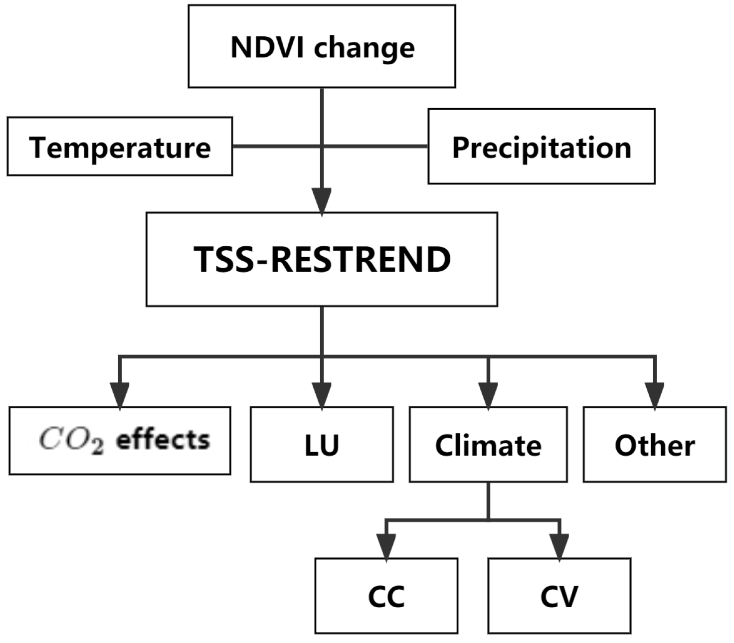
2.10. Dominant Factor Distribution

To investigate the regional dominant driving factor that affects the vegetation growth, we apply the ternary mapping of three main factors (CO 2 , LU, CC). The three limit conditions are linearly stretched in the range from 0 to 255, then assigned to red (CO 2 ), green (LU) and blue (CC). The color map can show the results of which driving factor is the dominant factor and the synergistic effects of three factors [33]. The ternary maps are plotted by the package of python-ternary.

3. Results

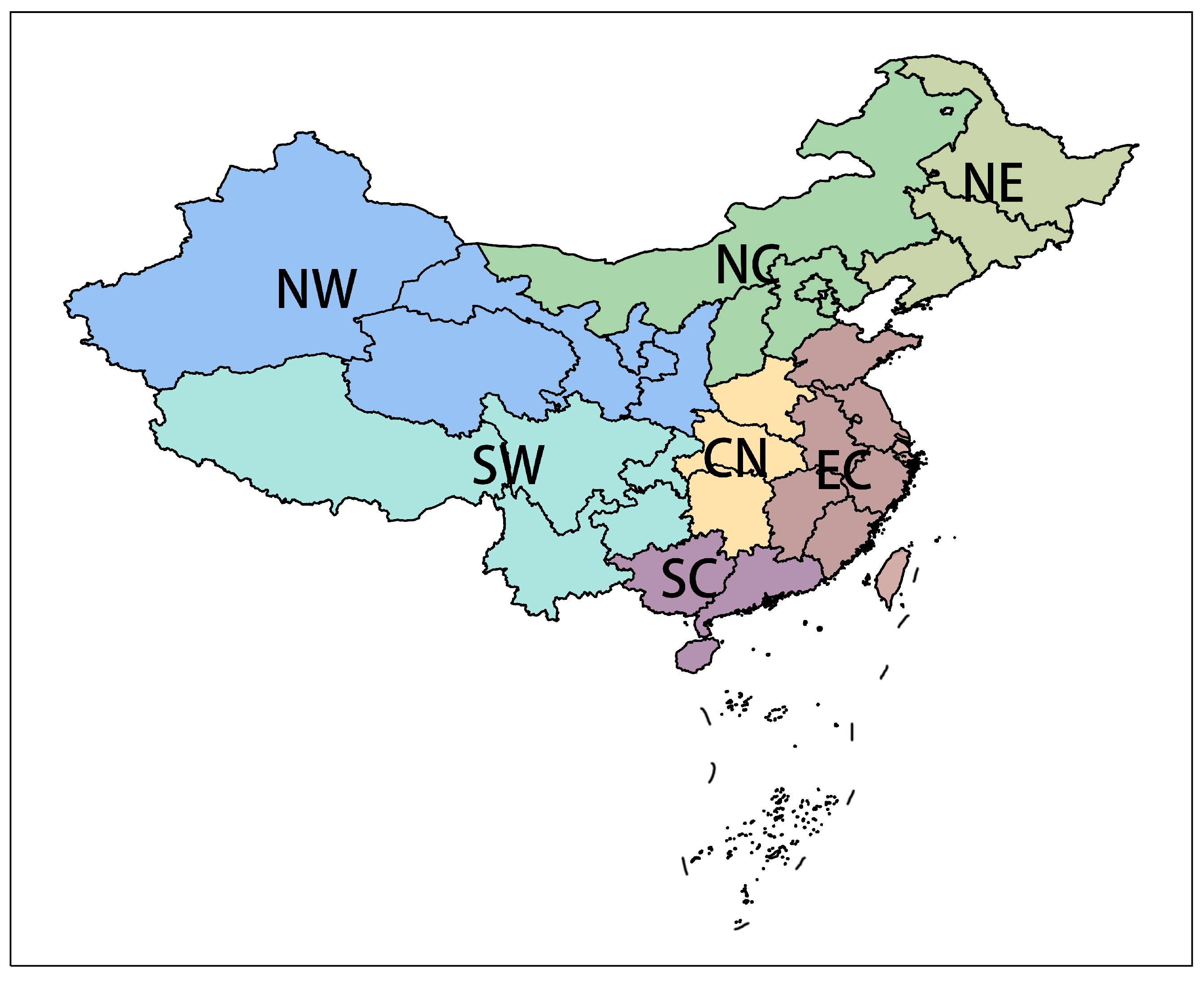
3.1. Dryland Areas in China

3.1.1. Detection and Attribution of Vegetation Growth

We identify the dry land of China through Arid Index. The areas are mainly located in the west and north of China (Figure 4). On the whole, most areas tend to be green over the past four decades (green area). However, desertification occurs in Xinjiang, Qinghai and Inner Mongolia (yellow area). We attribute the vegetation growth to mainly three driving factors (CO 2 fertilization effects, Land use, Climate change, Climate variability) and quantify the contributions of each one. We find that CO 2 fertilization has positive effects on all areas, especially in northeast China. This result is in line with previous studies that CO 2 fertilization effects are responsible for global green based on many observational evidences. For land use effects, they have negative effects mainly in Xinjiang, Qinghai and west Inner Mongolia. Overgrazing and urbanization account for most of the negative effects [34]. CC has positive effects chiefly in the west and negative effects in the northeast. The current internationally scientific point now is “dry areas get drier, wet areas get wetter”. However, Shi et al., (2002) found that the climate of arid regions in Northwest China are undergoing the shift from warm-dry to warm-wet, which shows that Chinese drylands are not in line with that hypothesis [35].

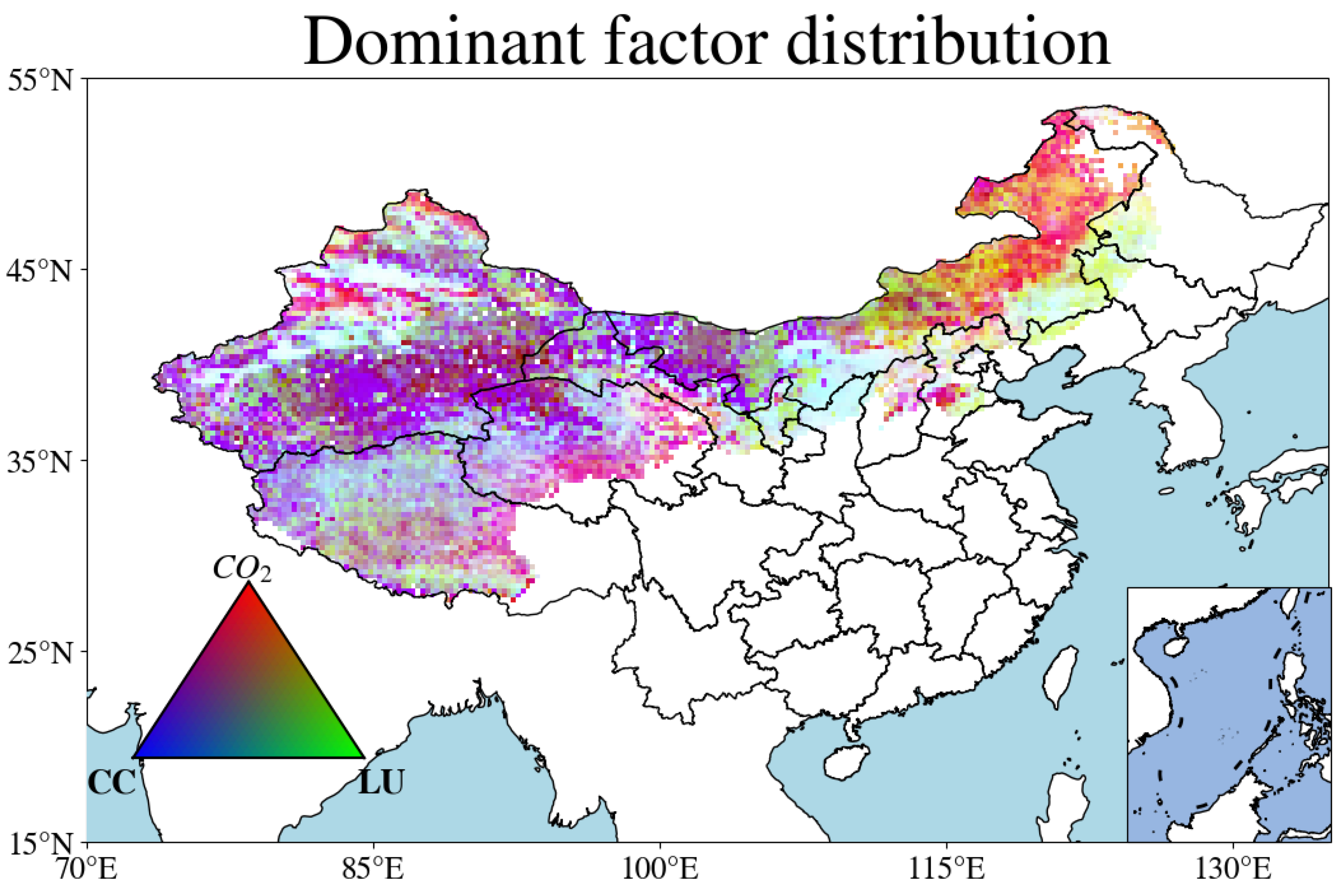
3.1.2. Dominant Factor Distribution

To investigate the dominant factors and synergistic effects of driving factors, we applied the ternary map of CO 2 (red), LU (green) and CC (blue). It can be seen in the Figure 5 that northeast China is mainly dominated by CO 2 fertilization effects. For the northwest, more regions are mainly controlled by CC. Many studies suggest that the northwest of China is undergoing a trend of wetter and warmer from the 1980s. Shi et al., (2002) found that the climate of arid regions in Northwest China are undergoing the shift from warm-dry to warm-wet. This research has aroused widespread concern [35]. Additionally, this change of climate is improving the environment of the northwest of China. Climate change has occurred longer than the 30 yr climatology and has influenced the ecological vegetation visibly [35]. Meanwhile, most color of the northwest is purple, which means CO 2 also has non-negligible effects. LU (green) shows a main effect in the middle of Inner Mongolia.

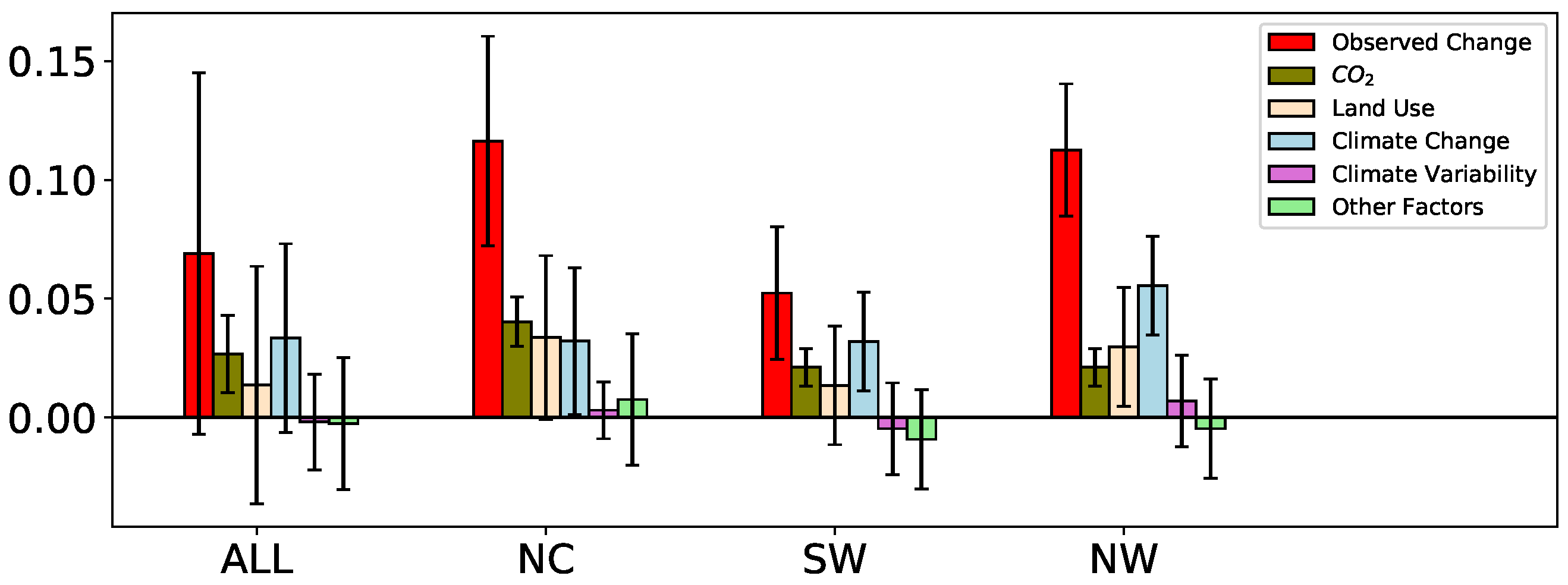
3.1.3. Region Analysis

We separate China into seven regions as in the figure and the dryland areas are mainly located in Northwest (NW), North China (NC), Northeast (NE) and Southwest (SW) (Figure 6). From Figure 7, we find that, in all dryland areas, CC contributes the most positive effects around 48.3%. This suggests that the vegetation in Chinese drylands is very sensitive to variations in temperature and precipitation, which is in agreement with Zhang (2021) [36]. The CO 2 fertilization effects contribute about 38.6%. There are differences between regions. For NC, the dominant factor is CO 2 accounting for 34.5%. LU and CC contribute almost the same effects (about 28.9% and 27.6%). For SW, CC has the most key role, accounting for about 61.0%. CV has negative effects, here accounting for about 9.2%. For NW, CC also has the most import role in vegetation growth (49.2%). From the figure, we conclude that the change of vegetation growth is affected by anthropogenic activities.

3.1.4. Drivers for Green and Desertification

We observed widespread green in Chinese drylands (Figure 8a). We find that CC is the dominant factor accounting for 44.5%. CO 2 and LU are a little smaller (35.3% and 26.1%). For NC, CO 2 plays the most important role here (35.1%). LU and CC are almost the same (28.7% and 27.7%). For SW and NW, the ecological vegetation is fairly sensitive to climate. Climatic warming and humidification here will obviously affect the vegetation. So, we conclude that CC is the dominant factor in the vegetation growth of SW and NW (61.3% and 46.8%). In the dryland that experienced desertification in China (Figure 8b), a negative component of LU is the dominant factor. Even though the average values of CC and CV are smaller than LU, climate plays an important role in desertification. For most areas, CC plays positive effects on vegetation growth.

3.2. Dryland Areas in America

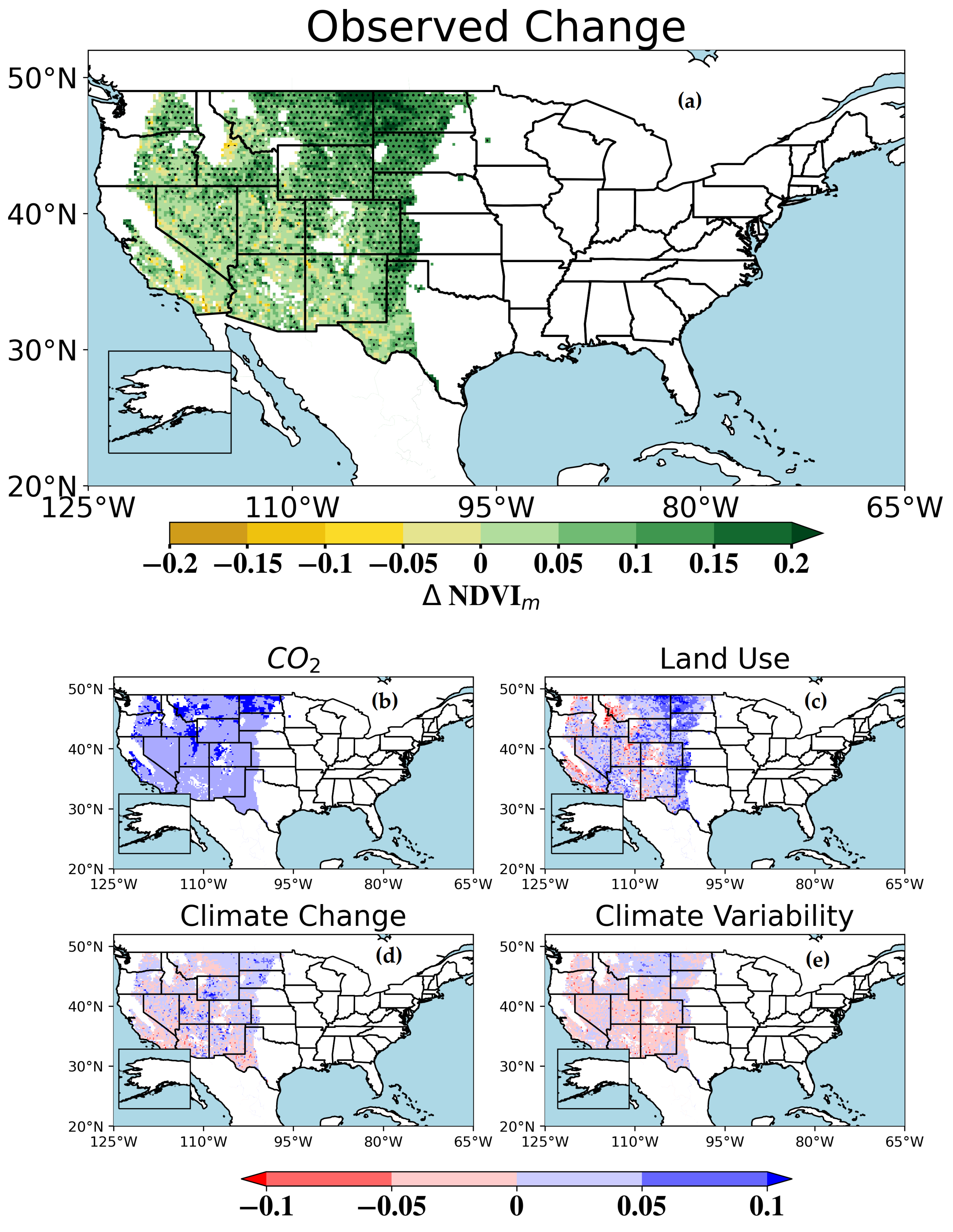
3.2.1. Detection and Attribution of Vegetation Growth

In the American dryland, most areas also show the significant greening trend except west and south areas (New Mexico, Arizona, California, Utah, Nevada, Idaho). The maximum and significant positive trend areas are mainly located in the north (Figure 9). CO 2 shows the obvious positive effects and impact on North Dakota. For most areas in Colorado, Kansas and California, LU shows negative effects. Overgrazing followed by nutrient depletion is considered by many studies as a cardinal element in land degradation in the west of the USA. Shrubs are viewed as mainly competitors when the grass is destroyed by overgrazing [14]. CC and CV show smaller effects than LU and CO 2 . For most areas, CV has negative effects on vegetation growth. Previous research found that there is a decrease in summer rains, which benefit grass growth, and a concomitant increase in winter rain, which benefits shrub rains in the drylands of the USA [11].

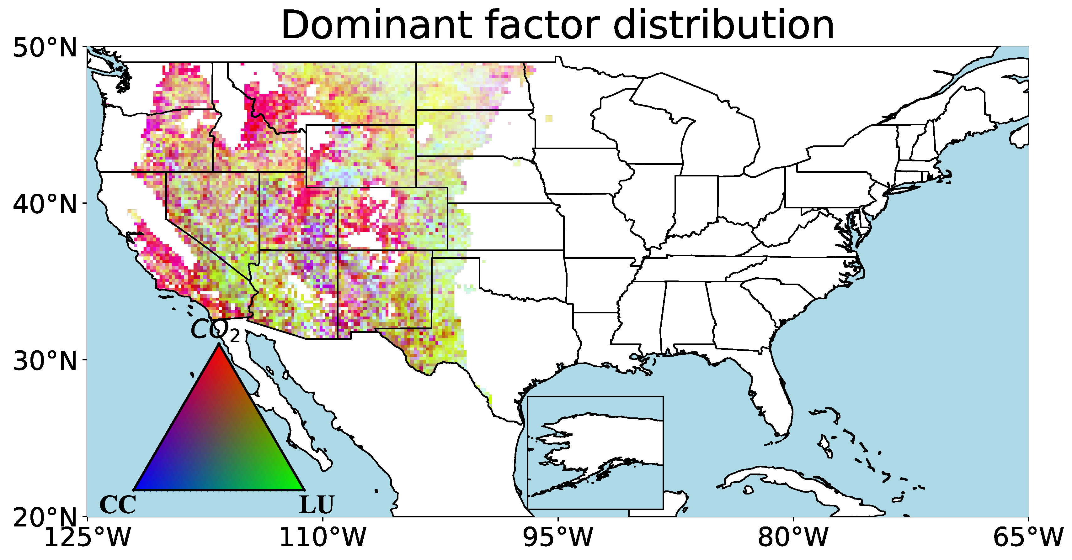
3.2.2. Dominant Factor Distribution

In this section, we discover the regional dominant factor of American drylands (Figure 10). We attributed the vegetation growth to three main factors (CO 2 , CC and LU). We found that most areas of American dryland were controlled by CO 2 and LU. Previous studies found that in some west areas such as New Mexico, grass predominated in the middle and end of the 19th century. However, the grass biomass decreased to less than 7% until the end of the 20th century due to overgrazing. This led to a shift in ecosystem structure and function here. Grass depletion led to nutrient loss and surface erodibility. The expanded shrub occupied the main plant biomass [37]. Additionally, the role of CC in vegetation change cannot be ignored. It is found that a change in the rain also contributed to the shift. The shrub expanded due to the temporal precipitation distribution characterized by a decrease in summer rains and the concomitant increase in winter rain [11].

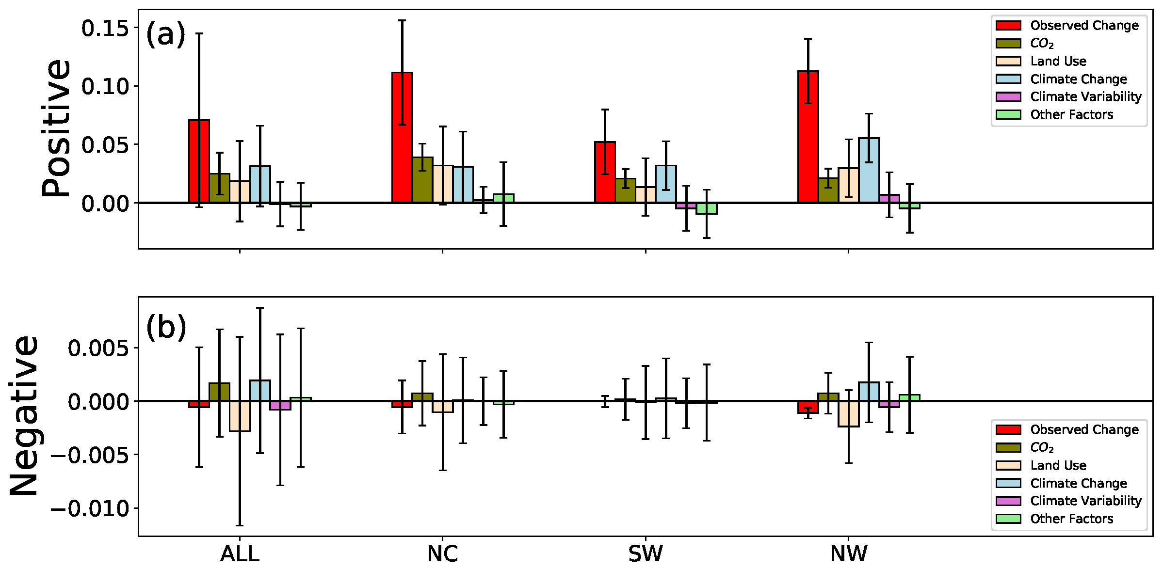
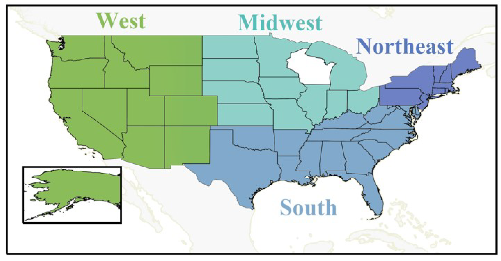
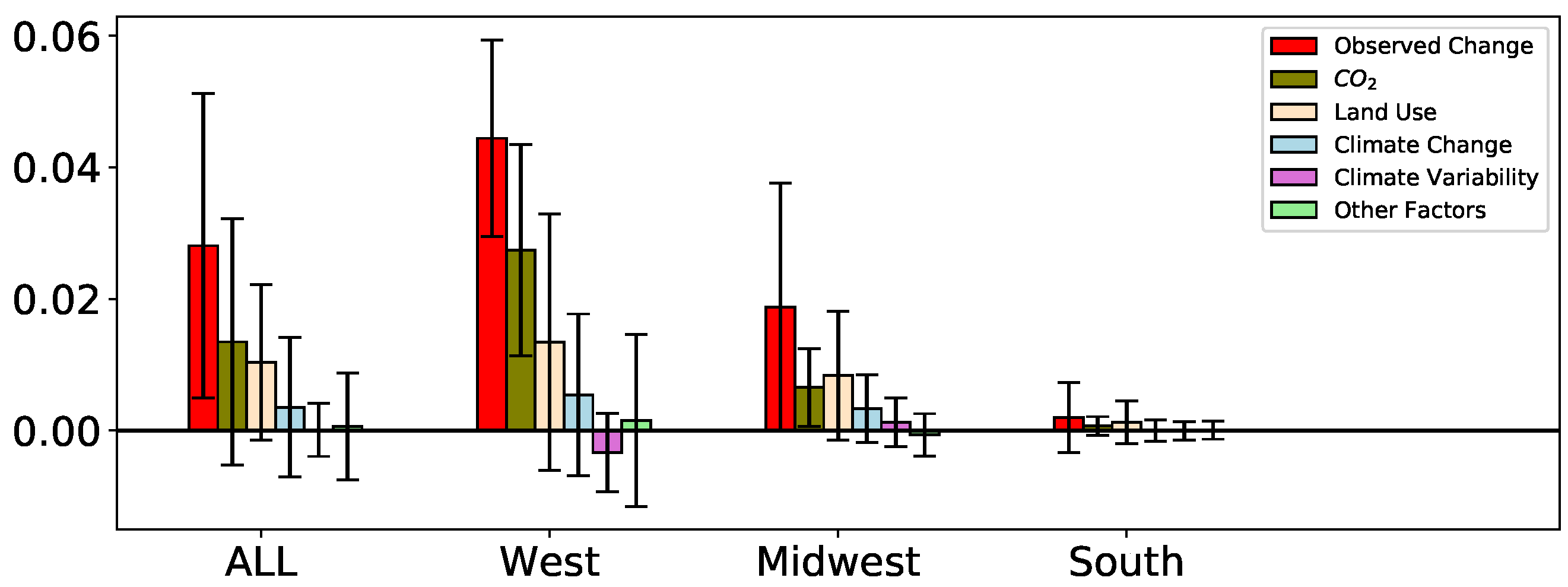
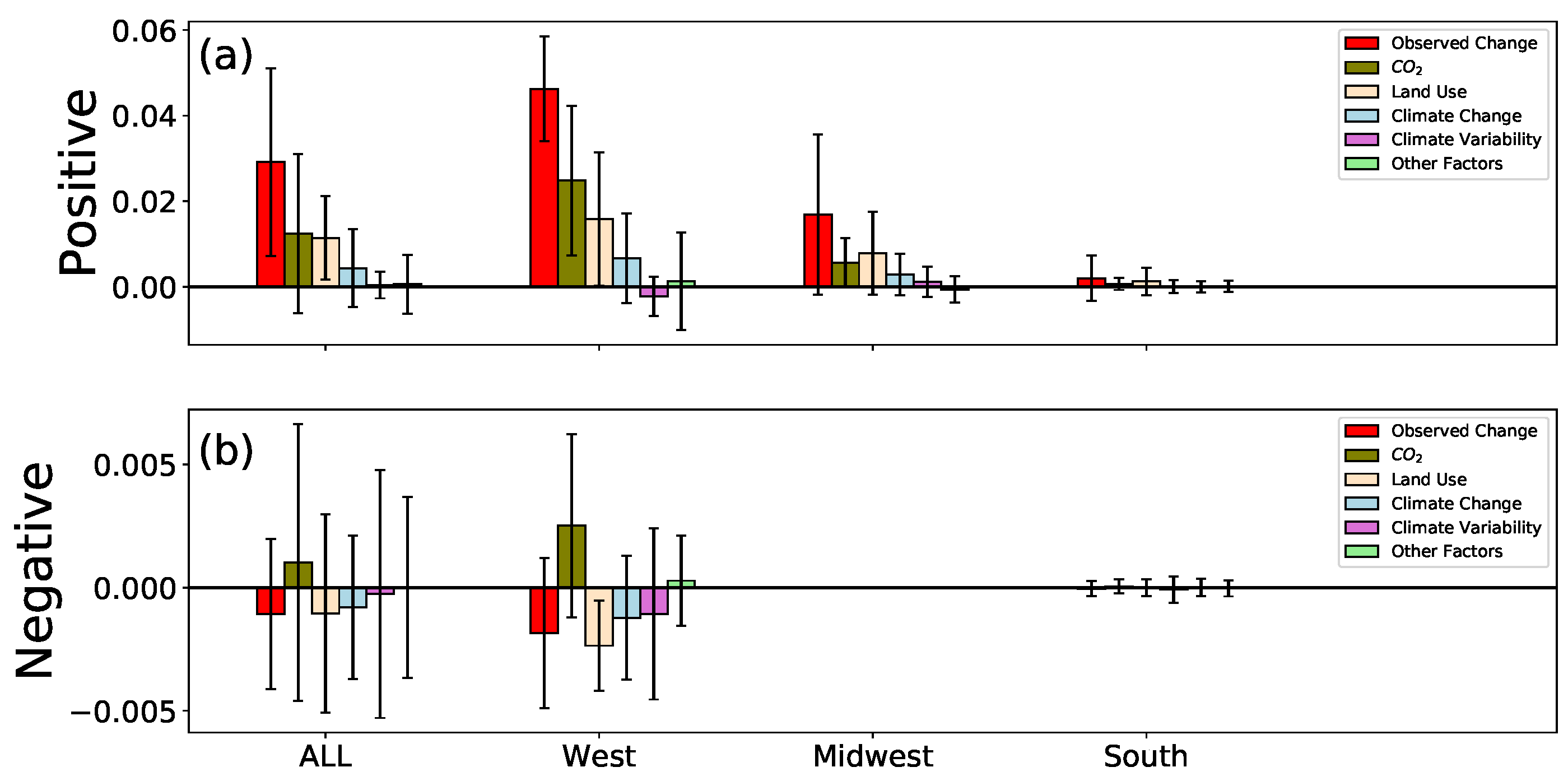
3.2.3. Region Analysis

We separated the USA into four regions (West, Midwest, Northeast and South). The dryland areas are mainly located in West, Midwest and South (Figure 11). We regionally attributed the vegetation growth to different factors such as CO 2 , CC, LU, CV and other factors our methods cannot attribute (Figure 12). For all American dryland areas, we found that CO 2 is the dominant factor accounting for 47.9%. LU accounts for 36.8%. Among the dryland areas, the West shows the most significant positive trend. CO 2 plays the most important role accounting for 61.7%, LU is 30.2%. It is notable that CV contributed negative effects on vegetation growth for 40 decades. For the Midwest, LU contributed the most on greening here, accounting for 44.6%. For the South, only a few areas are included in dryland and the observed change can be ignored.

3.2.4. Drivers for Green and Desertification

In this section, we analyzed the drivers for green and desertification of American dryland. Most areas show positive trend. CO 2 always shows positive effects (Figure 13a). For the whole dryland, CO 2 contributes the most, accounting for 42.9%. LU is a little less than CO 2 (39.3%). CC accounts for 14.8%. Among the three regions, the West shows apparently positive trend. Here, CO 2 is the primary driver in 53.7%. CV notably has negative effects on vegetation growth. For the Midwest, LU (46.4%) is the largest driver of change. We also observed some part of desertification areas. For the whole regions that experienced desertification, we found that LU is the largest attributed driver, followed by CC and CV. For the West, the positive effects of CO 2 almost offset the negative effects of LU. Even though the effects of CC and CV are a little smaller than LU and CO 2 , climate remains a significant driver of land degradation. In the West dryland, the land degradation expanded due to the temporal precipitation distribution characterized by a decrease in summer rains and the concomitant increase in winter rain [11].

4. Discussion

Our study is compared to two recent global studies by Song et al. [4] and Zhu et al. [38] that investigated the drivers of global vegetation change. Zhu et al. employed a 10-model ensemble and performed change attribution by running models with and without different drivers, then comparing the results. Meanwhile, Song et al. used AVHRR-derived vegetation fractions to analyze changes in vegetation types and used high-resolution imagery at 1500 locations worldwide to attribute the change. They identified visible signs of human activity at each location and attributed the observed change to land use if present, or to indirect drivers such as climate change if not. Both Song et al. and Zhu et al. have demonstrated the inconsistency that exists within the published literature, as they reveal large differences in attribution, while also highlighting the consistency in broad trends in vegetation change. While our study only focuses on the dryland biomes of China and America, it is worth noting that these global studies have used different spatial domains, which makes direct comparison challenging.
Zhu et al. found that nitrogen deposition was the second largest global driver, but this finding was uncertain since only two of their models could be run with and without nitrogen deposition. However, it is widely accepted that nitrogen deposition is not a significant driver of vegetation change in drylands. Recent research on the effects of nitrogen deposition on plant species showed that drylands are not responsive to increased nitrogen loads due to their overwhelming water limitation, and are predominantly located in regions with very low nitrogen deposition, except for a small part of the southwestern United States [39].

5. Conclusions

Dryland areas are undergoing changes under the influence of global warming. These ecosystems are fragile and extremely sensitive to external forces such as climate change and deforestation, which can significantly impact social and economic development. While there are many factors contributing to dryland ecosystem change, discovering the dominant factor that impacts each region and quantifying the effects of each factor remain worldwide hotspot issues.
In our study, through statistical methods, we disentangled the state of the ecosystem in Chinese and American dryland areas over the past 40 years. We attributed the vegetation change to CO 2 , land use (LU), climate change (CC), and climatic variability (CV) and quantified the effects of each factor on regional analysis. Additionally, we discovered the drivers for green and desertification regionally.
Our results showed that most of the Chinese and American dryland areas exhibit a greening trend, suggesting that the states of ecosystems in dryland areas are improving. However, desertification exists in some regions, such as Xinjiang, Qinghai, and Inner Mongolia in China and Colorado, Kansas, and California in the USA.
Furthermore, we found that the most dominant driver for vegetation changes in Chinese dryland areas is CC (48.3%), while CO 2 is the most dominant driver for the USA (47.9%). The primary factor of positive trends in America is the CO 2 fertilization effect (42.9%), while LU is the primary factor for desertification. For China, CC is the main driver for positive trends (35.3%), while LU is the primary driver for desertification. Our analysis for greening and desertification in each dryland area is summarized in Table 1.
All in all, our study highlights the importance of understanding the driving factors behind the green and land degradation of Chinese and American dryland areas. While our approach quantifies the impact of CO 2 , LU, CC, and CV on vegetation change, we acknowledge that there may be other factors at play, such as nitrogen deposition. Understanding the dominant factors can help prevent desertification and promote sustainable development in these areas.

Author Contributions

Z.C. and J.L. designed the study. X.H., P.F. and Z.Q. conducted the data and wrote the paper. L.L. and Z.Z. contributed to writing. G.S., B.L. and G.F. helped with validations. All authors have read and agreed to the published version of the manuscript.

Funding

This work was funded by the National Natural Science Foundation of China under Grant nos. 41975062. This work was funded by the National Natural Science Foundation of China under Grant nos. 42130610, 41905053, 42275034, 42075029, 41675050, and 11801398 and the Outstanding Young Talents Support Plan of Shanxi province.

Data Availability Statement

The NDVI dataset is from NOAA and can be accessed from https://www.ncei.noaa.gov/products/climate-data-records (accessed on 20 May 2023). We use a combination of a 9-member ensemble that consists of three precipitation and three temperature datasets. They are daily records of TerraClimate [http://www.climatologylab.org/terraclimate.html (accessed on 20 May 2023)], CRU4 [http://data.ceda.ac.uk//badc/cru/data/cru_ts/ (accessed on 20 May 2023)] and ERA5 [https://cds.climate.copernicus.eu/ (accessed on 20 May 2023)].

Conflicts of Interest

The authors declare no conflict of interest.

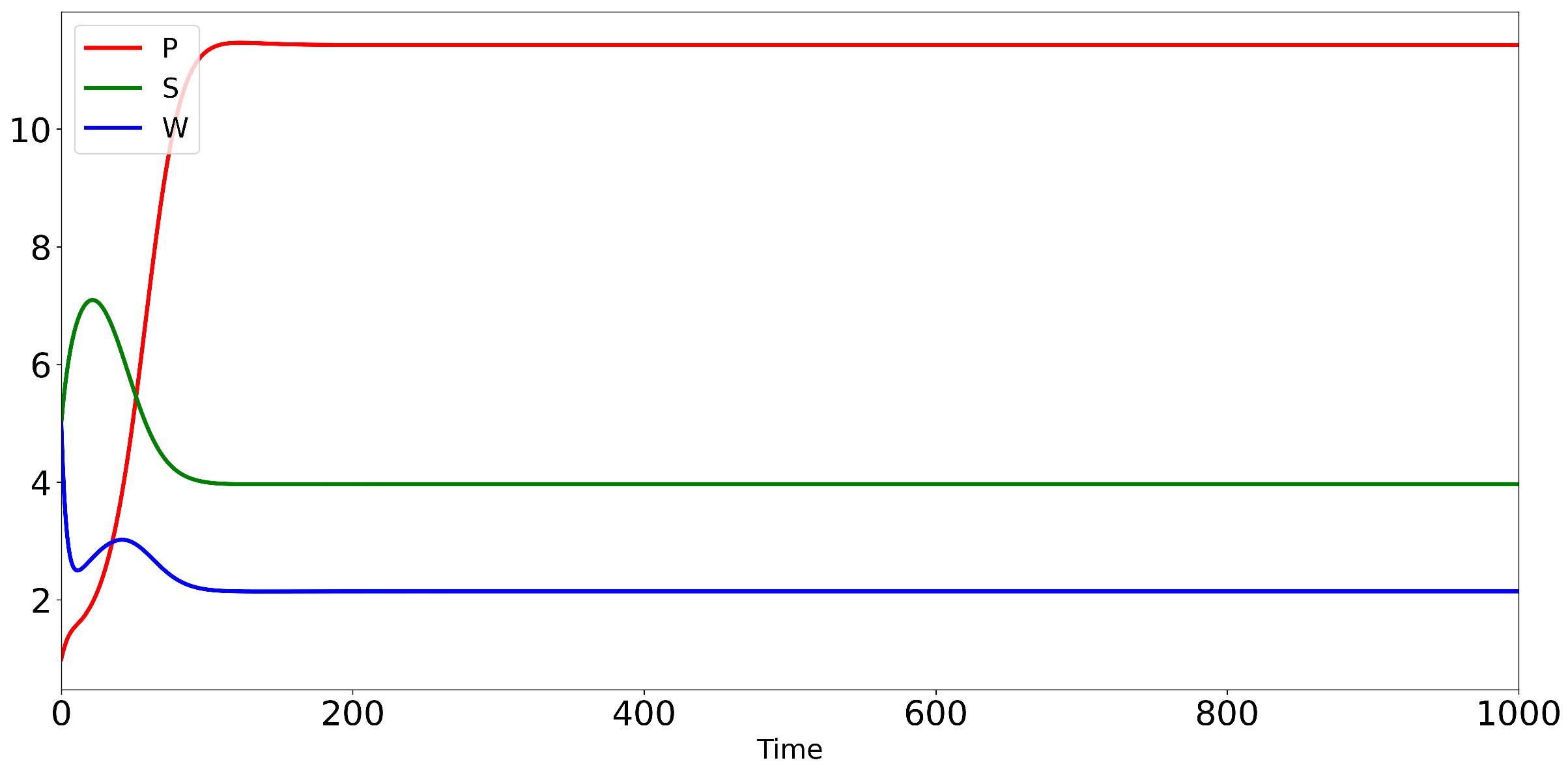
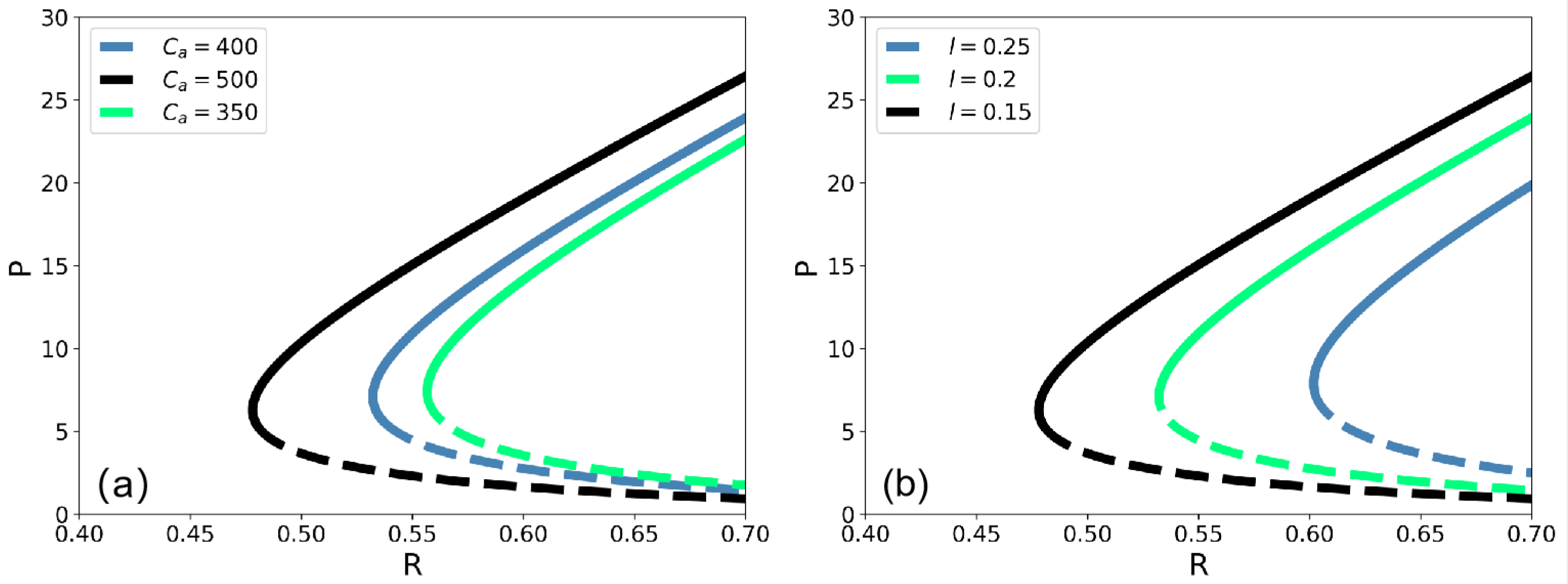
Appendix A. Model Description

Appendix A.1. Dynamic of Surface Water

When the rain falls to the ground, one part is left on the ground and the other part will infiltrate into the soil. The infiltration rate is based on the surface vegetation biomass because the vegetation reduces the surface crust and the root system increases the fraction sites of macro-pore sites near the soil surface. The dynamic of the surface water can be characterized as:
d S d t = R α S P + k 2 W o P + k 2 .
In which, R (mm/d) is the precipitation. α (d 1 ) is the maximum infiltration rate. k 2 (gm 2 ) is the water infiltration constant. W o is dimensionless, characterizing a measure of the infiltration contrast between vegetated and bare soil.

Appendix A.2. Dynamic of Soil Water

The water infiltrated from the surface is lost because of the plant absorption, evaporation or run-off.
d W d t = α S P + k 2 W o P + k 2 β W W + k 1 P r w W .
where β (mm g 1 m 2 d 1 ) is the maximum specific water uptake. r w (d 1 ) is the specific soil water loss because of evaporation and run-off. k 1 (mm d 1 ) is the half-saturation constant of vegetation growth and water uptake.

Appendix A.3. Dynamic of Vegetation Biomass

Plant growth and loss are characterized by carbon gain by photosynthesis, which depends on CO 2 concentration and land use change. The dynamic can be modeled by:
d P d t = c β W W + k 1 P l P .
where c = C a ( 1 C i C a ) C 1 describe the photosynthesis of vegetation. C a (mol mol 1 ) is the current CO 2 concentration. C i (mol mol 1 ) is the effective canopy intercellular concentration. C 1 (g mol 1 ) is the coefficient of conversion of photosynthesis (mol) into biomass (g). l (d 1 ) characterizes the land use rates such as grazing and land restoration.

Appendix B. Parameter Values Used

k 1 = 5 , k 2 = 5 , r w = 0.2 , W 0 = 0.2 , β = 0.05 , α = 0.2 , C 1 = 12 , C i = 0.6 C a .

References

  1. Kéfi, S.; Rietkerk, M.; Alados, C.L.; Pueyo, Y.; Papanastasis, V.P.; ElAich, A.; De Ruiter, P.C. Spatial vegetation patterns and imminent desertification in Mediterranean arid ecosystems. Nature 2007, 449, 213–217. [Google Scholar] [CrossRef] [PubMed]
  2. Reynolds, J.F.; Smith, D.M.S.; Lambin, E.F.; Turner, B.; Mortimore, M.; Batterbury, S.P.; Downing, T.E.; Dowlatabadi, H.; Fernández, R.J.; Herrick, J.E.; et al. Global desertification: Building a science for dryland development. Science 2007, 316, 847–851. [Google Scholar] [CrossRef] [PubMed]
  3. Klausmeier, C.A. Regular and irregular patterns in semiarid vegetation. Science 1999, 284, 1826–1828. [Google Scholar] [CrossRef]
  4. Song, X.P.; Hansen, M.C.; Stehman, S.V.; Potapov, P.V.; Tyukavina, A.; Vermote, E.F.; Townshend, J.R. Global land change from 1982 to 2016. Nature 2018, 560, 639–643. [Google Scholar] [CrossRef]
  5. Peng, S.; Chen, A.; Xu, L.; Cao, C.; Fang, J.; Myneni, R.B.; Pinzon, J.E.; Tucker, C.J.; Piao, S. Recent change of vegetation growth trend in China. Environ. Res. Lett. 2011, 6, 044027. [Google Scholar] [CrossRef]
  6. Kidron, G.J.; Gutschick, V.P. Temperature rise may explain grass depletion in the Chihuahuan Desert. Ecohydrology 2017, 10, e1849. [Google Scholar] [CrossRef]
  7. Liu, C.; Melack, J.; Tian, Y.; Huang, H.; Jiang, J.; Fu, X.; Zhang, Z. Detecting land degradation in eastern China grasslands with time series segmentation and residual trend analysis (TSS-RESTREND) and GIMMS NDVI3g data. Remote Sens. 2019, 11, 1014. [Google Scholar] [CrossRef]
  8. Piao, S.; Ciais, P.; Huang, Y.; Shen, Z.; Peng, S.; Li, J.; Zhou, L.; Liu, H.; Ma, Y.; Ding, Y.; et al. The impacts of climate change on water resources and agriculture in China. Nature 2010, 467, 43–51. [Google Scholar] [CrossRef] [PubMed]
  9. Niemand, C.; Köstner, B.; Prasse, H.; Grünwald, T.; Bernhofer, C. Relating tree phenology with annual carbon fluxes at. Meteorol. Z. 2005, 14, 197–202. [Google Scholar] [CrossRef]
  10. Piao, S.; Friedlingstein, P.; Ciais, P.; Viovy, N.; Demarty, J. Growing season extension and its impact on terrestrial carbon cycle in the Northern Hemisphere over the past 2 decades. Glob. Biogeochem. Cycles 2007, 21, GB3018. [Google Scholar] [CrossRef]
  11. Gibbens, R.; McNeely, R.; Havstad, K.; Beck, R.; Nolen, B. Vegetation changes in the Jornada Basin from 1858 to 1998. J. Arid. Environ. 2005, 61, 651–668. [Google Scholar] [CrossRef]
  12. Huenneke, L.F.; Anderson, J.P.; Remmenga, M.; Schlesinger, W.H. Desertification alters patterns of aboveground net primary production in Chihuahuan ecosystems. Glob. Chang. Biol. 2002, 8, 247–264. [Google Scholar] [CrossRef]
  13. Li, J.; Okin, G.S.; Alvarez, L.; Epstein, H. Quantitative effects of vegetation cover on wind erosion and soil nutrient loss in a desert grassland of southern New Mexico, USA. Biogeochemistry 2007, 85, 317–332. [Google Scholar] [CrossRef]
  14. Svejcar, L.N.; Bestelmeyer, B.T.; Duniway, M.C.; James, D.K. Scale-dependent feedbacks between patch size and plant reproduction in desert grassland. Ecosystems 2015, 18, 146–153. [Google Scholar] [CrossRef]
  15. Gottfried, M.; Pauli, H.; Futschik, A.; Akhalkatsi, M.; Barančok, P.; Benito Alonso, J.L.; Coldea, G.; Dick, J.; Erschbamer, B.; Fernández Calzado, M.a.R.; et al. Continent-wide response of mountain vegetation to climate change. Nat. Clim. Chang. 2012, 2, 111–115. [Google Scholar] [CrossRef]
  16. Fensham, R.; Fairfax, R.; Archer, S. Rainfall, land use and woody vegetation cover change in semi-arid Australian savanna. J. Ecol. 2005, 93, 596–606. [Google Scholar] [CrossRef]
  17. Sun, G.Q.; Wang, C.H.; Chang, L.L.; Wu, Y.P.; Li, L.; Jin, Z. Effects of feedback regulation on vegetation patterns in semi-arid environments. Appl. Math. Model. 2018, 61, 200–215. [Google Scholar] [CrossRef]
  18. Huang, J.; Yu, H.; Guan, X.; Wang, G.; Guo, R. Accelerated dryland expansion under climate change. Nat. Clim. Chang. 2016, 6, 166–171. [Google Scholar] [CrossRef]
  19. Li, J.; Sun, G.Q.; Jin, Z. Interactions of time delay and spatial diffusion induce the periodic oscillation of the vegetation system. Discret. Contin. Dyn.-Syst.-B 2021, 27, 2147–2172. [Google Scholar] [CrossRef]
  20. Chen, Z.; Liu, J.; Li, L.; Wu, Y.; Feng, G.; Qian, Z.; Sun, G.Q. Effects of climate change on vegetation patterns in Hulun Buir Grassland. Phys. Stat. Mech. Its Appl. 2022, 597, 127275. [Google Scholar] [CrossRef]
  21. Li, J.; Sun, G.Q.; Guo, Z.G. Bifurcation analysis of an extended Klausmeier–Gray–Scott model with infiltration delay. Stud. Appl. Math. 2022, 148, 1519–1542. [Google Scholar] [CrossRef]
  22. Qiu, Y.; Xu, Z.; Xu, C.; Holmgren, M. Can remotely sensed vegetation patterns signal dryland restoration success? Restor. Ecol. 2022, 31, e13760. [Google Scholar] [CrossRef]
  23. Chen, Z.; Wu, Y.P.; Feng, G.L.; Qian, Z.H.; Sun, G.Q. Effects of global warming on pattern dynamics of vegetation: Wuwei in China as a case. Appl. Math. Comput. 2021, 390, 125666. [Google Scholar] [CrossRef]
  24. Kefi, S.; Rietkerk, M.; Katul, G.G. Vegetation pattern shift as a result of rising atmospheric CO2 in arid ecosystems. Theor. Popul. Biol. 2008, 74, 332–344. [Google Scholar] [CrossRef]
  25. Sun, G.Q.; Zhang, H.T.; Song, Y.L.; Li, L.; Jin, Z. Dynamic analysis of a plant-water model with spatial diffusion. J. Differ. Equations 2022, 329, 395–430. [Google Scholar] [CrossRef]
  26. Tian, F.; Brandt, M.; Liu, Y.Y.; Verger, A.; Tagesson, T.; Diouf, A.A.; Rasmussen, K.; Mbow, C.; Wang, Y.; Fensholt, R. Remote sensing of vegetation dynamics in drylands: Evaluating vegetation optical depth (VOD) using AVHRR NDVI and in situ green biomass data over West African Sahel. Remote. Sens. Environ. 2016, 177, 265–276. [Google Scholar] [CrossRef]
  27. Tebaldi, C.; Arblaster, J.M.; Knutti, R. Mapping model agreement on future climate projections. Geophys. Res. Lett. 2011, 38, L23701. [Google Scholar] [CrossRef]
  28. Meinshausen, M.; Smith, S.J.; Calvin, K.; Daniel, J.S.; Kainuma, M.L.; Lamarque, J.F.; Matsumoto, K.; Montzka, S.A.; Raper, S.C.; Riahi, K.; et al. The RCP greenhouse gas concentrations and their extensions from 1765 to 2300. Clim. Chang. 2011, 109, 213–241. [Google Scholar] [CrossRef]
  29. Burrell, A.; Evans, J.; De Kauwe, M. Anthropogenic climate change has driven over 5 million km2 of drylands towards desertification. Nat. Commun. 2020, 11, 3853. [Google Scholar] [CrossRef]
  30. Franks, P.J.; Adams, M.A.; Amthor, J.S.; Barbour, M.M.; Berry, J.A.; Ellsworth, D.S.; Farquhar, G.D.; Ghannoum, O.; Lloyd, J.; McDowell, N.; et al. Sensitivity of plants to changing atmospheric CO2 concentration: From the geological past to the next century. New Phytol. 2013, 197, 1077–1094. [Google Scholar] [CrossRef]
  31. Burrell, A.L.; Evans, J.P.; Liu, Y. Detecting dryland degradation using time series segmentation and residual trend analysis (TSS-RESTREND). Remote Sens. Environ. 2017, 197, 43–57. [Google Scholar] [CrossRef]
  32. Burrell, A.L.; Evans, J.P.; Liu, Y. The addition of temperature to the TSS-RESTREND methodology significantly improves the detection of dryland degradation. IEEE J. Sel. Top. Appl. Earth Obs. Remote Sens. 2019, 12, 2342–2348. [Google Scholar] [CrossRef]
  33. Nemani, R.R.; Keeling, C.D.; Hashimoto, H.; Jolly, W.M.; Piper, S.C.; Tucker, C.J.; Myneni, R.B.; Running, S.W. Climate-driven increases in global terrestrial net primary production from 1982 to 1999. Science 2003, 300, 1560–1563. [Google Scholar] [CrossRef] [PubMed]
  34. Liu, Y.Y.; Evans, J.P.; McCabe, M.F.; de Jeu, R.A.; van Dijk, A.I.; Dolman, A.J.; Saizen, I. Changing climate and overgrazing are decimating Mongolian steppes. PLoS ONE 2013, 8, e57599. [Google Scholar] [CrossRef] [PubMed]
  35. Shi, Y.; Shen, Y.; Hu, R. Preliminary study on signal, impact and foreground of climatic shift from warm–dry to warm–humid in Northwest China (in Chinese). J. Glaciol. Geocryol. 2002, 24, 219–226. [Google Scholar]
  36. Zhang, Q.; Yang, J.; Wang, W.; Ma, P.; Lu, G.; Liu, X.; Yu, H.; Fang, F. Climatic warming and humidification in the arid region of Northwest China: Multi-scale characteristics and impacts on ecological vegetation. J. Meteorol. Res. 2021, 35, 113–127. [Google Scholar] [CrossRef]
  37. Viglizzo, E.F.; Nosetto, M.D.; Jobbágy, E.G.; Ricard, M.F.; Frank, F.C. The ecohydrology of ecosystem transitions: A meta-analysis. Ecohydrology 2015, 8, 911–921. [Google Scholar] [CrossRef]
  38. Zhu, Z.; Piao, S.; Myneni, R.B.; Huang, M.; Zeng, Z.; Canadell, J.G.; Ciais, P.; Sitch, S.; Friedlingstein, P.; Arneth, A.; et al. Greening of the Earth and its drivers. Nat. Clim. Chang. 2016, 6, 791–795. [Google Scholar] [CrossRef]
  39. Bobbink, R.; Hicks, K.; Galloway, J.; Spranger, T.; Alkemade, R.; Ashmore, M.; Bustamante, M.; Cinderby, S.; Davidson, E.; Dentener, F.; et al. Global assessment of nitrogen deposition effects on terrestrial plant diversity: A synthesis. Ecol. Appl. 2010, 20, 30–59. [Google Scholar] [CrossRef]
Figure 1. Evolution of vegetation biomass, surface water and soil water. R = 0.6 , l = 0.15 , C a = 400 . Other parameters are shown in Appendix A.
Remotesensing 15 02688 g001
Figure 2. Sensitive analysis of different factors. (a) is for CO 2 and (b) is for land use rate. Solid line is the stable state and dotted line is the unstable state. There exists one bifurcation when the system approaches a certain value under different climate conditions.
Remotesensing 15 02688 g002
Figure 3. Flowchart of the methods.
Remotesensing 15 02688 g003
Figure 4. (a) Observed change of vegetation growth in Chinese dryland area. Yellow means decrease in NDVI m and green means increase. Dotted areas suggest the change is significant ( α F D R = 0.10). Areas that have large uncertainties are masked in white. (b) The change of NDVI attributed to CO 2 . (c) The change of NDVI attributed to LU. (d) The change of NDVI attributed to CC. (e) The change of NDVI attributed to CV.
Remotesensing 15 02688 g004
Figure 5. Map of three dominant factors distribution in Chinese dryland areas. The areas controlled by CO 2 are shown in red. The areas controlled by LU are shown in green. The areas controlled by CC is shown in blue.
Remotesensing 15 02688 g005
Figure 6. Regional separation for analysis of China. Chinese dryland areas mainly locate in Northwest (NW), North China (NC) and Southwest (SW).
Remotesensing 15 02688 g006
Figure 7. The regional mean and magnitude (mean absolute value) of the different drivers of change in NDVI m of Chinese dryland areas. The error bars show the SD of grid cells.
Remotesensing 15 02688 g007
Figure 8. (a) The regional mean and magnitude (mean absolute value) of the different drivers of positive change in NDVI m of Chinese dryland areas. The error bars show the SD of grid cells. (b) The same as (a) for negative change.
Remotesensing 15 02688 g008
Figure 9. (a) Observed change of vegetation growth in American dryland area. Yellow means decrease in NDVI m and green means increase. Dotted areas suggest the change is significant ( α F D R = 0.10). Areas that have large uncertainties are masked in white. (b) The change of NDVI m attributed to CO 2 . (c) The change of NDVI m attributed to LU. (d) The change of NDVI m attributed to CC. (e) The change of NDVI m attributed to CV.
Remotesensing 15 02688 g009
Figure 10. Map of three dominant factors’ distribution in American dryland areas. The areas controlled by CO 2 are shown in red. The areas controlled by LU are shown in green. The areas controlled by CC are shown in blue.
Remotesensing 15 02688 g010
Figure 11. Regional separation for analysis of America. American dryland areas mainly locate in West, Midwest and South.
Remotesensing 15 02688 g011
Figure 12. The regional mean and magnitude (mean absolute value) of the different drivers of change in NDVI m of American dryland areas. The error bars show the SD of grid cells.
Remotesensing 15 02688 g012
Figure 13. (a) The regional mean and magnitude (mean absolute value) of the different drivers of positive change in NDVI m of American dryland areas. The error bars show the SD of grid cells. (b) The same as (a) for negative change.
Remotesensing 15 02688 g013
Table 1. Descriptions of detection and attribution on dryland areas in China and America.
Dryland Areas of ChinaDryland Areas of America
1
Most areas show a green trend over the past decades. However, there exists desertification in Xinjiang, Qinghai and Inner Mongolia of China.
1
Most areas show a green trend over the past decades. Desertification mainly exists in Colorado, Kansas and California.
2
The most dominant driver for vegetation changes in Chinese dryland areas is CC. China is undergoing fast development. Urbanization has changed most areas from a natural state to cities.
2
The most dominant driver for America is CO 2 fertilization effects.
3
The main driver for positive trends is CC. However, the primary driver for desertification is LU.
3
The primary factor for positive trends is the CO 2 fertilization effect. For desertification, LU is the primary factor. Overgrazing is also an unignorable factor for desertification.
Disclaimer/Publisher’s Note: The statements, opinions and data contained in all publications are solely those of the individual author(s) and contributor(s) and not of MDPI and/or the editor(s). MDPI and/or the editor(s) disclaim responsibility for any injury to people or property resulting from any ideas, methods, instructions or products referred to in the content.

