
Large-Scale Urban Heating and Pollution Domes over the Indian Subcontinent

Abstract
:1. Introduction
2. Materials and Methods
2.1. Data Sources
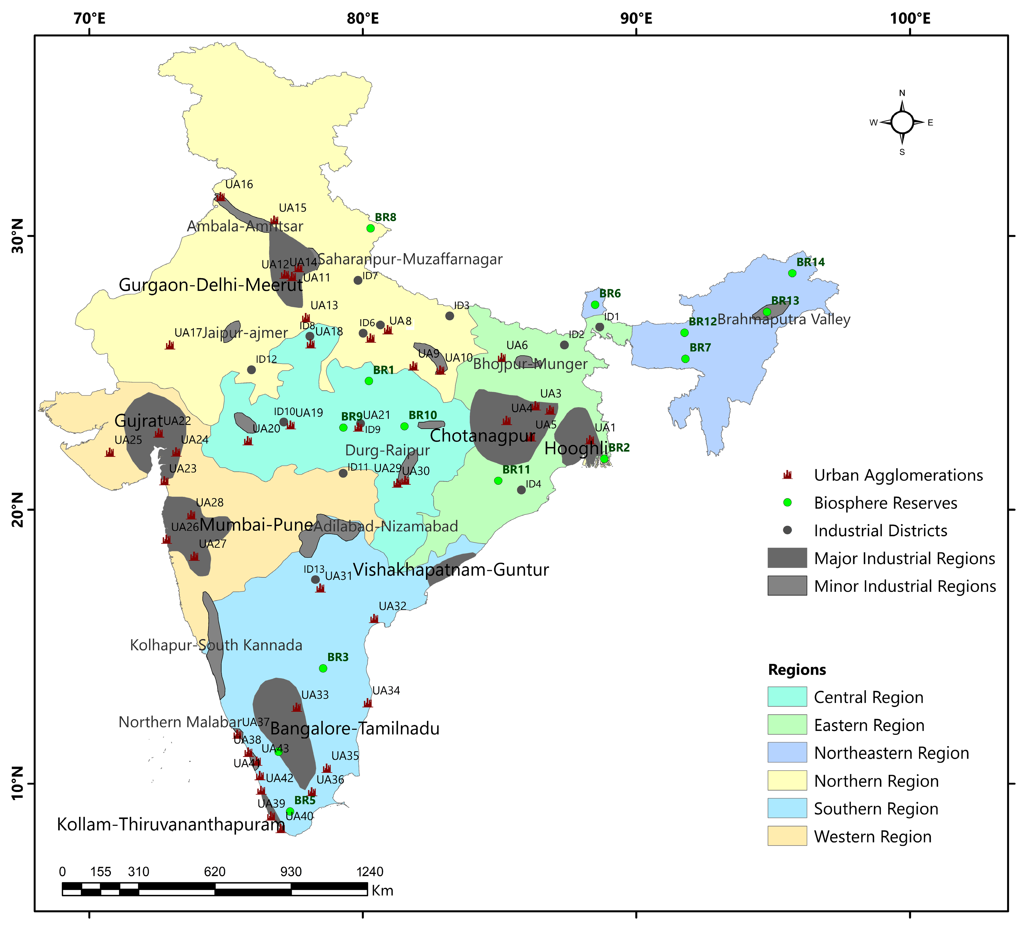
2.2. Data Mapping
2.3. Data Analysis
3. Results and Discussion
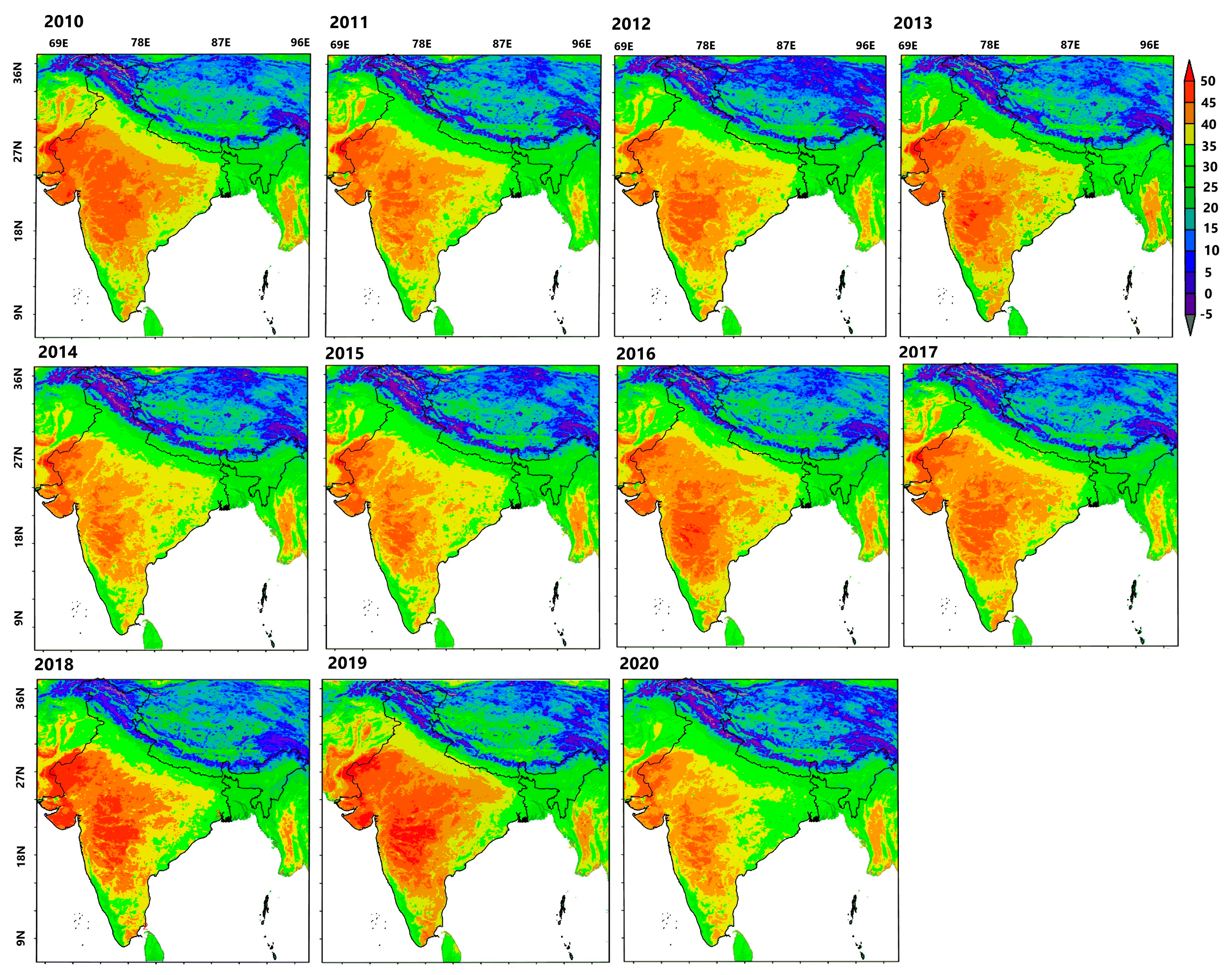
3.1. Pre-Monsoon Aerosol Optical Depth (AOD)
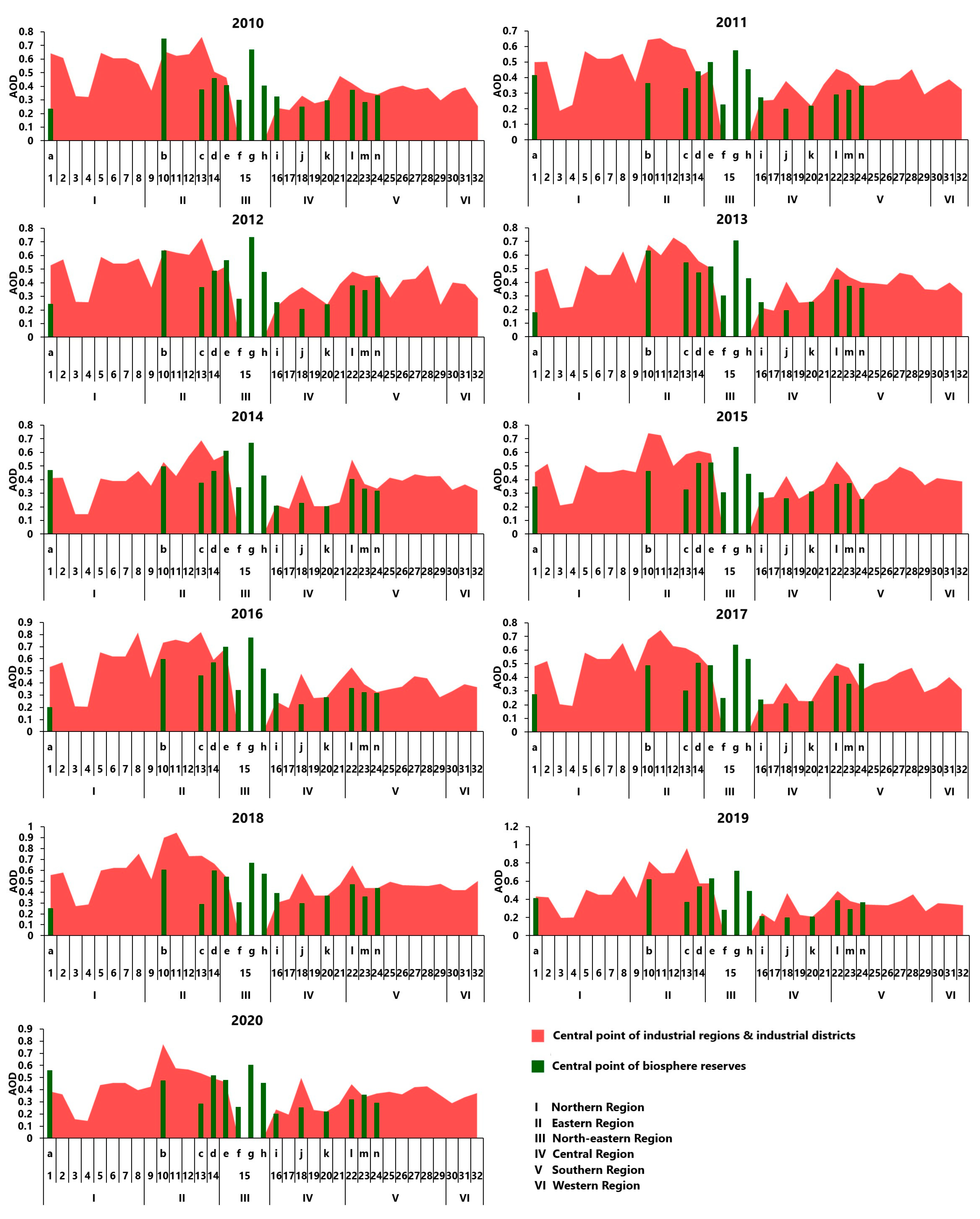
3.1.1. Spatiotemporal Comparison of Aerosol Optical Depth (AOD) for Industrial Regions (IDs) and Biosphere Reserves (BRs)
3.1.2. Pre-Monsoon Aerosol Optical Depth (AOD) Level of Urban Agglomerations (UAs) and Industrial Districts (IDs)
3.1.3. Pre-Monsoon Land Surface Temperatures (LSTs) in Urban Areas and Their Characteristics
3.1.4. Annual Pre-Monsoon Land Surface Temperature (LST) Level Percentage Change
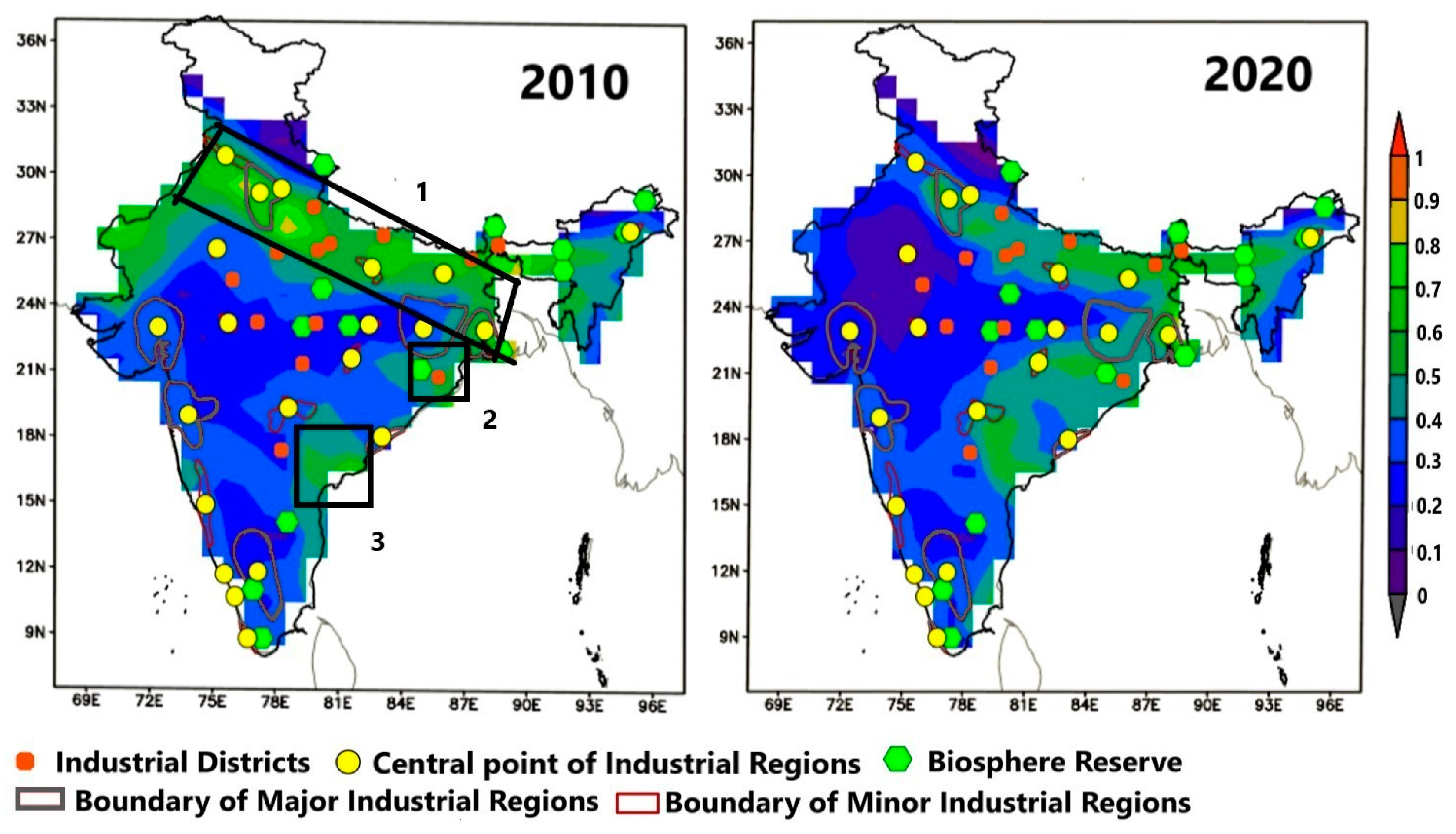
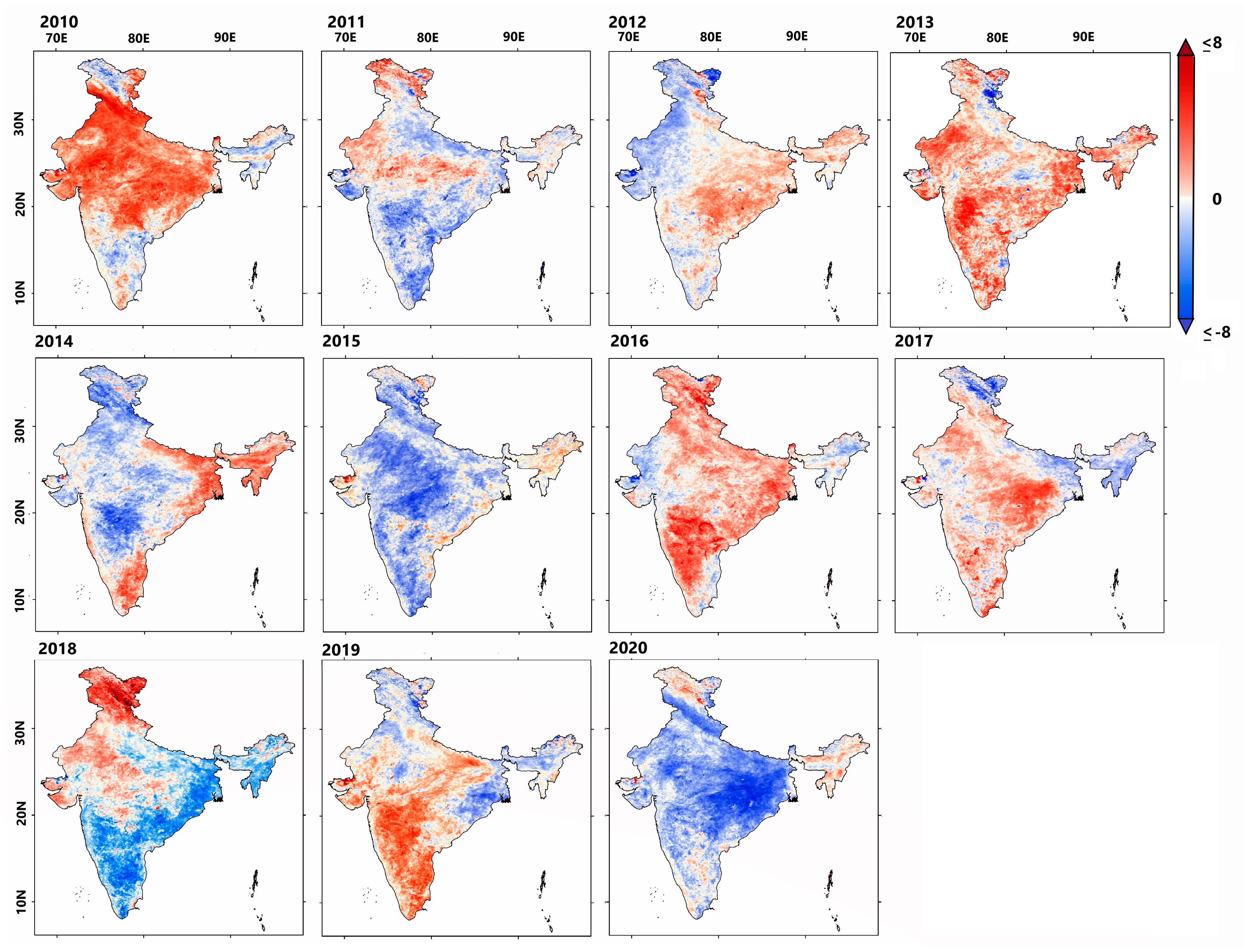
3.1.5. Land Surface Temperatures (LST) Anomaly Map Showing Increasing and Decreasing Trends during Pre-Monsoon (March–May) Season in India 2010–2020
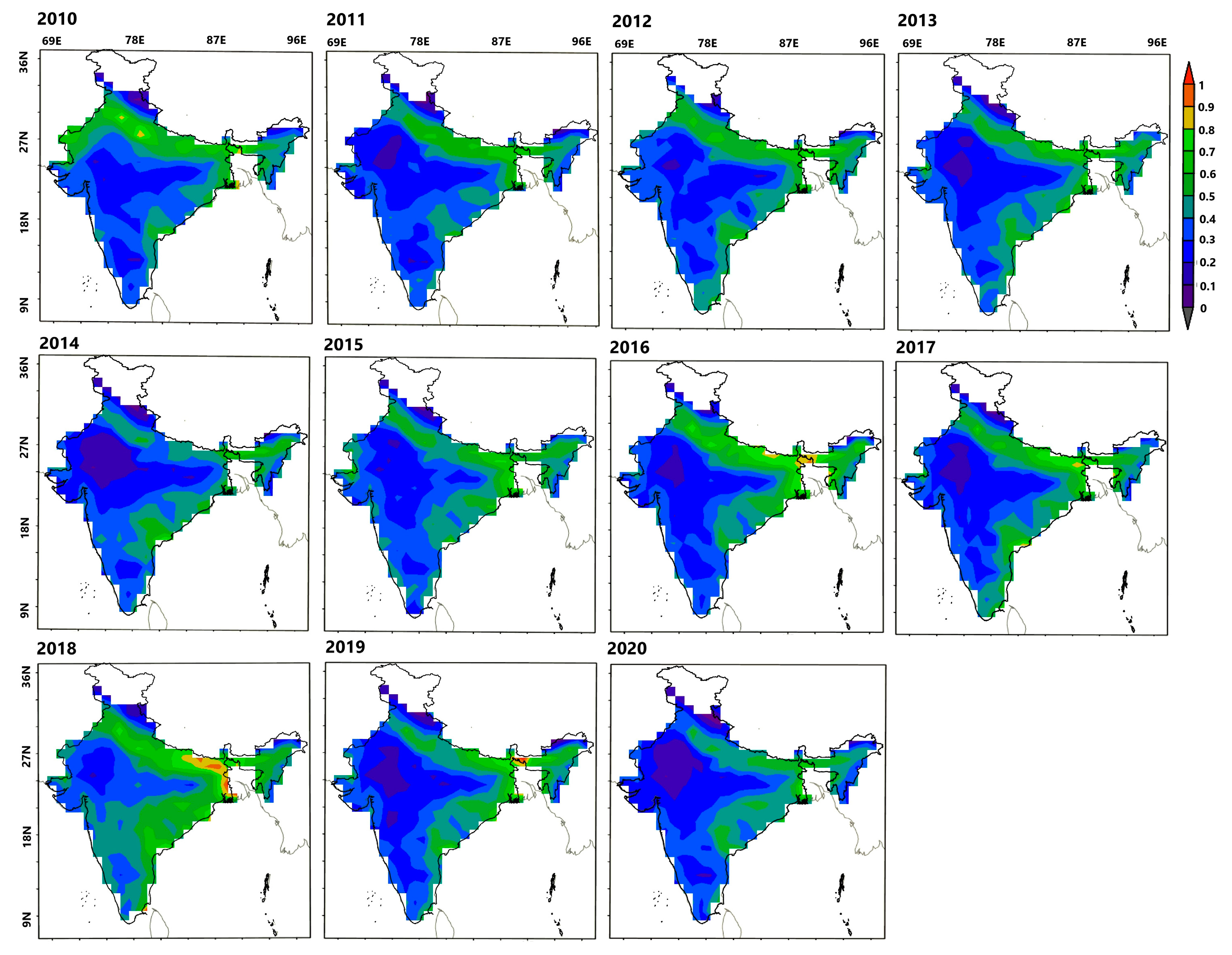
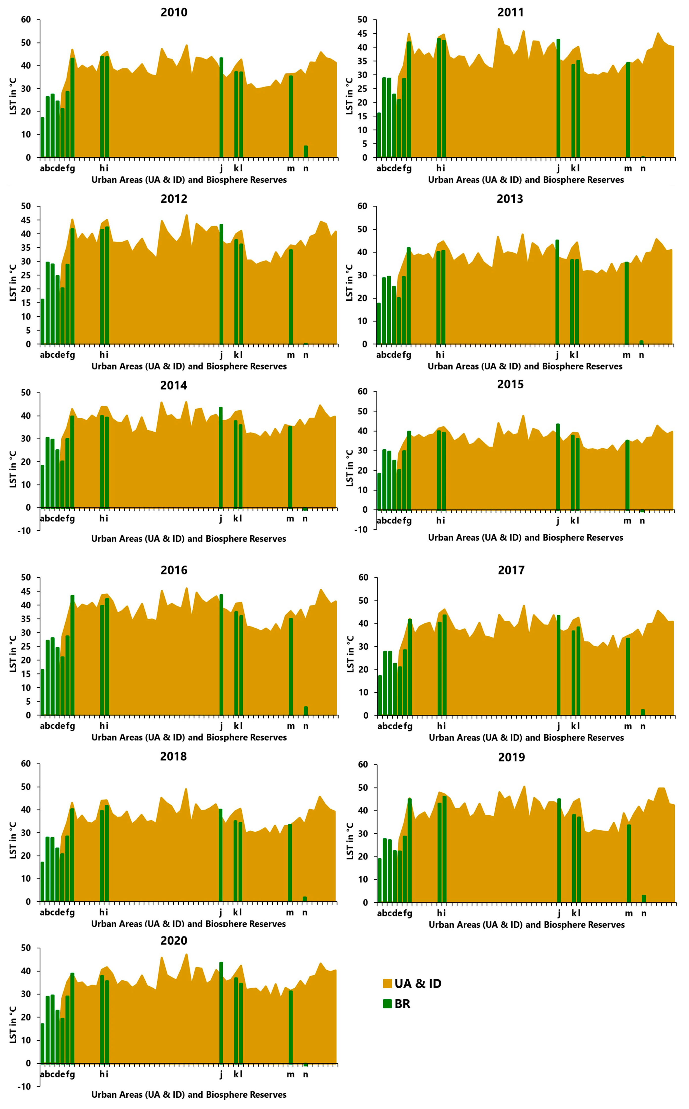
3.1.6. Year-Wise LST of Urban Agglomerations (UAs), Industrial Districts (IDs), and Biosphere Reserves (BRs)
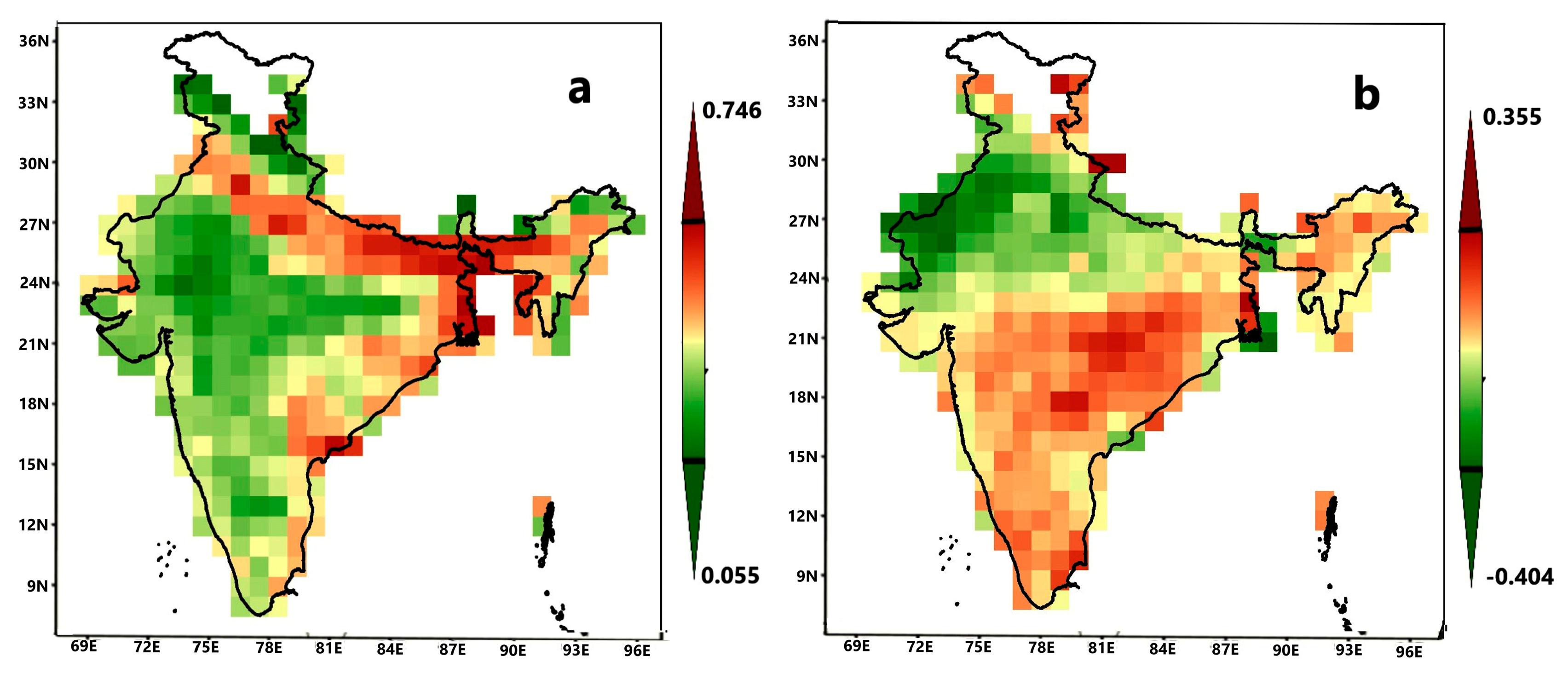
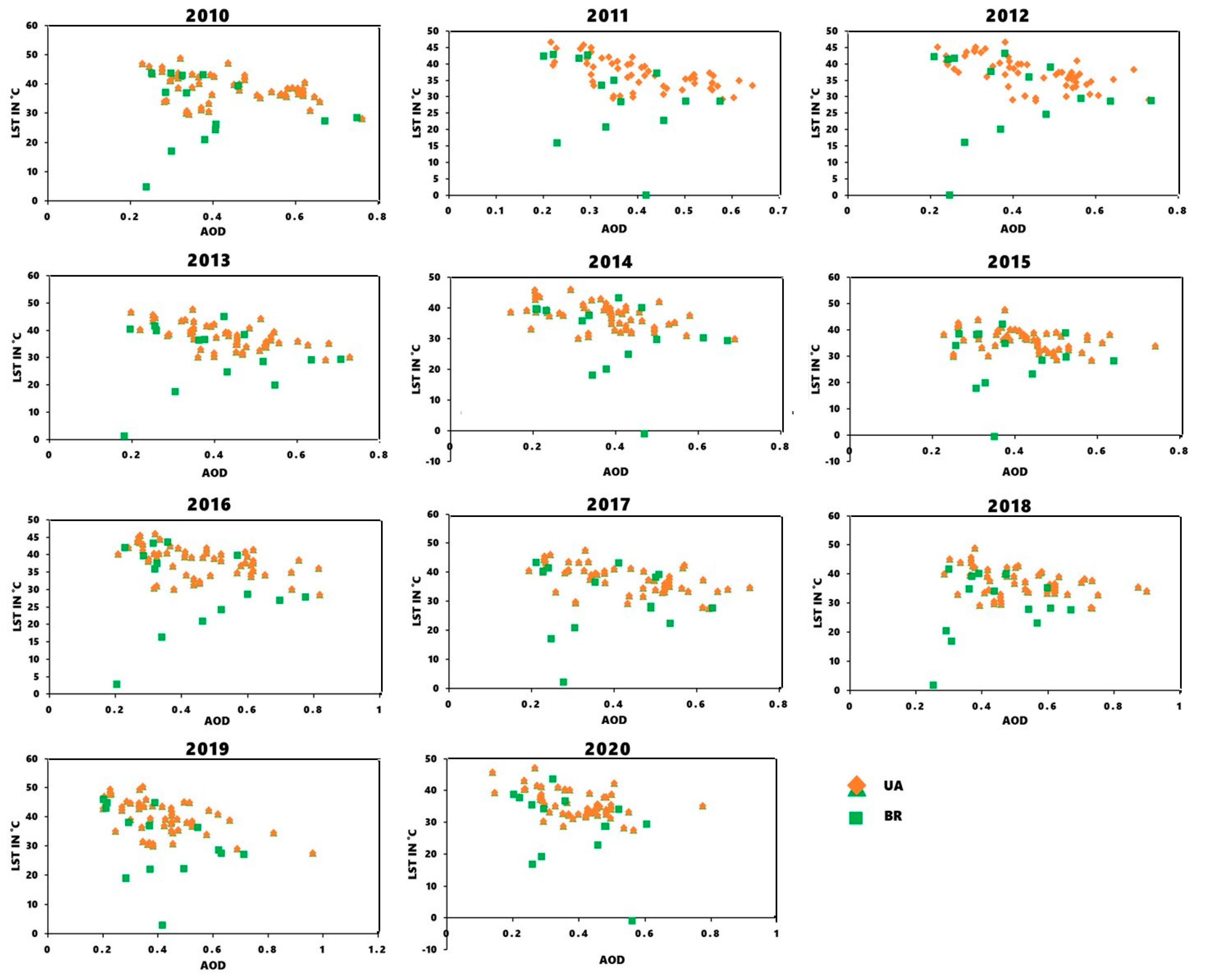
3.2. Pre-Monsoonal Relationship between Land Surface Temperature (LST) and Aerosol Optical Depth (AOD) in the Indian Subcontinent
4. Conclusions
Supplementary Materials
Author Contributions
Funding
Data Availability Statement
Acknowledgments
Conflicts of Interest
References
- Crutzen, P.J. New Directions: The growing urban heat and pollution “island” effect—Impact on chemistry and climate. Atmos. Environ. 2004, 38, 3539–3540. [Google Scholar] [CrossRef]
- Balakrishnan, K.; Dey, S.; Gupta, T.; Dhaliwal, R.S.; Brauer, M.; Cohen, A.J.; Stanaway, J.D.; Beig, G.; Joshi, T.K.; Aggarwal, A.N.; et al. The impact of air pollution on deaths, disease burden, and life expectancy across the states of India: The Global Burden of Disease Study 2017. Lancet Planet. Health 2019, 3, e26–e39. [Google Scholar] [CrossRef] [PubMed]
- Khan, A.; Khorat, S.; Khatun, R.; VanDoan, Q.; Nair, U.S.; Niyogi, D. Variable impact of COVID-19 lockdown on air quality across 91 Indian cities. Earth Interact. 2021, 25, 57–75. [Google Scholar] [CrossRef]
- Global Burden of Disease Collaborative Network. Global Burden of Disease Study 2016 (GBD 2016); Institute for Health Metrics and Evaluation (IHME): Seattle, WA, USA, 2017. [Google Scholar]
- Ramanathan, V.; Crutzen, P.J.; Kiehl, J.T.; Rosenfeld, D. Atmosphere: Aerosols, climate, and the hydrological cycle. Science 2001, 294, 2119–2124. [Google Scholar] [CrossRef]
- Wang, H.; Shi, G.Y.; Zhang, X.Y.; Gong, S.L.; Tan, S.C.; Chen, B.; Che, H.Z.; Li, T. Mesoscale modeling study of the interactions between aerosols and PBL meteorology during a haze episode in China Jing-Jin-Ji and its near surrounding region-Part 2: Aerosols’ radiative feedback effects. Atmos. Chem. Phys. Discuss. 2014, 14, 28269–28298. [Google Scholar] [CrossRef]
- Wang, Z.; Lin, L.; Yang, M.; Guo, Z. The Role of Anthropogenic Aerosol Forcing in Interdecadal Variations of Summertime Upper-Tropospheric Temperature Over East Asia. Earth’s Future 2019, 7, 136–150. [Google Scholar] [CrossRef]
- Das, S.; Giorgi, F.; Giuliani, G.; Dey, S.; Coppola, E. Near-Future Anthropogenic Aerosol Emission Scenarios and Their Direct Radiative Effects on the Present-Day Characteristics of the Indian Summer Monsoon. J. Geophys. Res. Atmos. 2020, 125, e2019JD031414. [Google Scholar] [CrossRef]
- Grey, I.; Arora, T.; Thomas, J.; Saneh, A.; Tohme, P.; Abi-habib, R. Since January 2020 Elsevier has created a COVID-19 resource centre with free information in English and Mandarin on the novel coronavirus COVID-19. The COVID-19 resource centre is hosted on Elsevier Connect, the company’ s public news and information. Psychiatry Res. 2020, 14, 293. [Google Scholar]
- Merikanto, J.; Nordling, K.; Räisänen, P.; Räisänen, J.; O’donnell, D.; Partanen, A.I.; Korhonen, H. How Asian aerosols impact regional surface temperatures across the globe. Atmos. Chem. Phys. 2021, 21, 5865–5881. [Google Scholar] [CrossRef]
- Kumar, R.; Barth, M.C.; Pfister, G.G.; Naja, M.; Brasseur, G.P. WRF-Chem simulations of a typical pre-monsoon dust storm in northern India: Influences on aerosol optical properties and radiation budget. Atmos. Chem. Phys. 2014, 14, 2431–2446. [Google Scholar] [CrossRef]
- Ginoux, P.; Prospero, J.M.; Gill, T.E.; Hsu, N.C.; Zhao, M. Global-scale attribution of anthropogenic and natural dust sources and their emission rates based on MODIS Deep Blue aerosol products. Rev. Geophys. 2012, 50, 1–36. [Google Scholar] [CrossRef]
- Prasad, A.K.; Singh, S.; Chauhan, S.S.; Srivastava, M.K.; Singh, R.P.; Singh, R. Aerosol radiative forcing over the Indo-Gangetic plains during major dust storms. Atmos. Environ. 2007, 41, 6289–6301. [Google Scholar] [CrossRef]
- Pan, X.; Chin, M.; Gautam, R.; Bian, H.; Kim, D.; Colarco, P.R.; Diehl, T.L.; Takemura, T.; Pozzoli, L.; Tsigaridis, K.; et al. A multi-model evaluation of aerosols over South Asia: Common problems and possible causes. Atmos. Chem. Phys. 2015, 15, 5903–5928. [Google Scholar] [CrossRef]
- Roy, S.S. Impact of aerosol optical depth on seasonal temperatures in India: A spatio-temporal analysis. Int. J. Remote Sens. 2008, 29, 727–740. [Google Scholar] [CrossRef]
- Kothawale, D.R.; Revadekar, J.V.; Kumar, K.R. Recent trends in pre-monsoon daily temperature extremes over India. J. Earth Syst. Sci. 2010, 119, 51–65. [Google Scholar] [CrossRef]
- Available online: https://mausam.imd.gov.in/imd_latest/contents/ar2020.pdf (accessed on 25 May 2022).
- Keramitsoglou, I.; Daglis, I.A.; Amiridis, V.; Chrysoulakis, N.; Ceriola, G.; Manunta, P.; Maiheu, B.; De Ridder, K.; Lauwaet, D.; Paganini, M. Evaluation of satellite-derived products for the characterization of the urban thermal environment. J. Appl. Remote Sens. 2012, 6, 061704. [Google Scholar] [CrossRef]
- Chakraborty, K.; Raju, P.L.N. Remote sensing technique-a tool for environmental studies. ADBU J. Eng. Technol. Chakraborty 2017, 6, 1–6. [Google Scholar]
- Pandey, P.; Kumar, D.; Prakash, A.; Kumar, K.; Jain, V.K. A Study of the Summertime Urban Heat Island over Delhi. Int. J. Sustain. Sci. Stud. 2009, 1, 27–34. [Google Scholar]
- Li, H.; Meier, F.; Lee, X.; Chakraborty, T.; Liu, J.; Schaap, M.; Sodoudi, S. Interaction between Urban Heat Island and Urban Pollution Island during Summer in Berlin. Sci. Total Environ. 2018, 636, 818–828. [Google Scholar] [CrossRef]
- Sussman, H.S.; Ajay Raghavendra, A.; Zhou, L. Impacts of increased urbanization on surface temperature, vegetation, and aerosols over Bengaluru, India. Remote Sens. Appl. Soc. Environ. 2019, 16, 100261. [Google Scholar] [CrossRef]
- Sarthi, P.P.; Kumar, S.; Barat, A.; Kumar, P.; Sinha, A.K.; Goswami, V. Linkage of Aerosol Optical Depth with Rainfall and Circulation Parameters over the Eastern Gangetic Plains of India. J. Earth Syst. Sci. 2019, 128, 171. [Google Scholar] [CrossRef]
- Han, W.; Li, Z.; Wu, F.; Zhang, Y.; Guo, J.; Su, T.; Cribb, M.; Fan, J.; Chen, T.; Wei, J.; et al. The Mechanisms and Seasonal Differences of the Impact of Aerosols on Daytime Surface Urban Heat Island Effect. Atmos. Chem. Phys. 2020, 20, 6479–6493. [Google Scholar] [CrossRef]
- AlFaisal, A.; Rahman, M.M.; Haque, S. Retrieving Spatial Variation of Aerosol Level over Urban Mixed Land Surfaces Using Landsat Imageries: Degree of Air Pollution in Dhaka Metropolitan Area. Phys. Chem. Earth 2022, 126, 103074. [Google Scholar] [CrossRef]
- Mal, S.; Rani, S.; Maharana, P. Estimation of Spatio-Temporal Variability in Land Surface Temperature over the Ganga River Basin Using MODIS Data. Geocarto Int. 2022, 37, 3817–3839. [Google Scholar] [CrossRef]
- Mielonen, T.; Hienola, A.; Merikanto, J.; Lipponen, A.; Laakso, A.; Bergman, T.; Korhonen, H.; Kolmonen, P.; Ghent, D.; Arola, A.; et al. The Climatic Significance of Biogenic Aerosols in the Boreal Region Now and in the Future. Authorea Prepr. 2018, 5–6. [Google Scholar] [CrossRef]
- Census 2021-Formation of Urban Agglomerations.pdf. Available online: https://censusindia.gov.in/nada/index.php/catalog/40512/download/44144/ORGI_circular003_2021.pdf (accessed on 1 January 2023).
- Putnik, D.G.; Cruz-Cunha, M.M. Encyclopedia of Networked and Virtual Organizations (3 Volumes); IGI Global: Hershey, PA, USA, 2008. [Google Scholar] [CrossRef]
- Available online: https://msme.gov.in/ (accessed on 1 January 2022).
- Available online: https://en.unesco.org/biosphere/about/ (accessed on 1 January 2023).
- Available online: https://en.unesco.org/biosphere/aspac/nokrek (accessed on 28 April 2023).
- Available online: https://en.unesco.org/biosphere/aspac/pachmarhi (accessed on 28 April 2023).
- Available online: https://en.unesco.org/biosphere/aspac/achanakmar-amarkantak (accessed on 28 April 2023).
- Available online: https://fsi.nic.in/forest-report-2021-details (accessed on 28 April 2023).
- Acker, J.G.; Leptoukh, G. Online analysis enhances use of NASA Earth Science Data. Eos Trans. Am. Geophys. Union 2007, 88, 14–17. [Google Scholar] [CrossRef]
- Available online: https://giovanni.gsfc.nasa.gov/giovanni/ (accessed on 20 May 2022).
- Available online: http://cola.gmu.edu/grads/ (accessed on 2 March 2022).
- Aftab, H.; Mansoor, A.B.; Asim, M. A New Single Image Interpolation Technique for Super Resolution. In Proceedings of the 2008 IEEE International Multitopic Conference, Karachi, Pakistan, 23–24 December 2008; pp. 592–596. [Google Scholar] [CrossRef]
- Setianto, A.; Triandini, T. Comparison of Kriging and Inverse Distance Weighted (Idw) Interpolation Methods in Lineament Extraction and Analysis. J. Appl. Geol. 2015, 5, 21–29. [Google Scholar] [CrossRef]
- Spearman, C. The Proof and Measurement of Association between Two Things. Am. J. Psychol. 1904, 15, 72–101. [Google Scholar] [CrossRef]
- Zar, J.H. Significance Testing of the Spearman Rank Correlation Coefficient. J. Am. Stat. Assoc. 1972, 67, 578–580. [Google Scholar] [CrossRef]
- Acharya, P.; Sreekesh, S. Seasonal variability in aerosol optical depth over India: A spatio-temporal analysis using the MODIS aerosol product. Int. J. Remote Sens. 2013, 34, 4832–4849. [Google Scholar] [CrossRef]
- Singh, N.; Mhawish, A.; Deboudt, K.; Singh, R.S.; Banerjee, T. Organic aerosols over Indo-Gangetic Plain: Sources, distributions and climatic implications. Atmos. Environ. 2017, 157, 59–74. [Google Scholar] [CrossRef]
- Gautam, R.; Hsu, N.C.; Lau, K.M.; Tsay, S.C.; Kafatos, M. Enhanced pre-monsoon warming over the Himalayan-Gangetic region from 1979 to 2007. Geophys. Res. Lett. 2009, 36, 1–5. [Google Scholar] [CrossRef]
- Gautam, R.; Hsu, N.C.; Tsay, S.C.; Lau, K.M.; Holben, B.; Bell, S.; Smirnov, A.; Li, C.; Hansell, R.; Ji, Q.; et al. Accumulation of aerosols over the Indo-Gangetic plains and southern slopes of the Himalayas: Distribution, properties and radiative effects during the 2009 pre-monsoon season. Atmos. Chem. Phys. 2011, 11, 12841–12863. [Google Scholar] [CrossRef]
- Dey, S.; Rongali, G. Aerosol Climatology and Intercomparison. In Satellite Meteoreology and Remote Sensing; Indian Institute of Technology: Delhi, India, 2014; pp. 1–17. Available online: https://web.iitd.ac.in/~sagnik/SN1.pdf (accessed on 2 January 2023).
- Grimmond, S. Urbanization and global environmental change: Local effects of urban warming. Geogr. J. 2007, 173, 83–88. [Google Scholar] [CrossRef]
- Grimmond, C.S.B.; Ward, H.C.; Kotthaus, S. How is urbanization altering local and regional climate? In The Routledge Handbook of Urbanization and Global Environmental Change; Routledge: New York, NY, USA, 2016; pp. 1–10. [Google Scholar]
- Hamdi, R.; Kusaka, H.; Van Doan, Q.; Cai, P.; He, H.; Luo, G.; Kuang, W.; Caluwaerts, S.; Duchêne, F.; Van Schaeybroek, B.; et al. The State-of-the-Art of Urban Climate Change Modeling and Observations. Earth Syst. Environ. 2020, 4, 631–646. [Google Scholar] [CrossRef]
- Kumar, R.; Mishra, V.; Buzan, J.; Kumar, R.; Shindell, D.; Huber, M. Dominant control of agriculture and irrigation on urban heat island in India. Sci. Rep. 2017, 7, 14054. [Google Scholar] [CrossRef]
- Hadibasyir, H.Z.; Rijal, S.S.; Sari, D.R. Comparison of Land Surface Temperature During and Before the Emergence of Covid-19 using Modis Imagery in Wuhan City, China. Forum Geogr. 2020, 34, 1–15. [Google Scholar] [CrossRef]
- Nanda, D.; Mishra, D.R.; Swain, D. COVID-19 lockdowns induced land surface temperature variability in mega urban agglomerations in India. Environ. Sci. Processes Impacts 2021, 23, 144–159. [Google Scholar] [CrossRef]
- Gupta, A.; Bhatt, C.M.; Roy, A.; Chauhan, P. COVID-19 Lockdown a Window of Opportunity to Understand the Role of Human Activity on Forest Fire Incidences in the Western Himalaya, India. Curr. Sci. 2020, 119, 390. [Google Scholar] [CrossRef]
- Bala, G.; Caldeira, K.; Wickett, M.; Phillips, T.J.; Lobell, D.B.; Delire, C.; Mirin, A. Combined Climate and Carbon-Cycle Effects of Large-Scale Deforestation. Proc. Natl. Acad. Sci. USA 2007, 104, 6550–6555. [Google Scholar] [CrossRef]
- Betts, R.A. Offset of the Potential Carbon Sink from Boreal Forestation by Decreases in Surface Albedo. Nature 2000, 408, 187–190. [Google Scholar] [CrossRef] [PubMed]
- Marland, G.; Pielke, R.A.; Apps, M.; Avissar, R.; Betts, R.A.; Davis, K.J.; Frumhoff, P.C.; Jackson, S.T.; Joyce, L.A.; Kauppi, P.; et al. The Climatic Impacts of Land Surface Change and Carbon Management, and the Implications for Climate-Change Mitigation Policy. Clim. Policy 2003, 3, 149–157. [Google Scholar] [CrossRef]
- Peng, S.; Piao, S.; Zeng, Z.; Ciais, P.; Zhou, L.; Li, L.Z.X.; Myneni, R.B. Afforestation in China Cools Local Land Surface Temperature. Proc. Natl. Acad. Sci. USA 2014, 111, 2915–2919. [Google Scholar] [CrossRef] [PubMed]
- Available online: https://www.britannica.com/place/Seshachalam-Hills/ (accessed on 3 March 2023).
- Jin, M.; Shepherd, J.M.; Zheng, W. Urban Surface Temperature Reduction via the Urban Aerosol Direct Effect: A Remote Sensing and WRF Model Sensitivity Study. Adv. Meteorol. 2010, 2010, 681587. [Google Scholar] [CrossRef]


| Code | Urban Agglomeration | Population | Code | Urban Agglomeration | Population |
|---|---|---|---|---|---|
| UA1 | Kolkata | 14,112,536 | UA23 | Surat | 4,585,367 |
| UA2 | Asansol | 1,243,008 | UA24 | Vadodara | 1,817,191 |
| UA3 | Dhanbad | 1,195,298 | UA25 | Rajkot | 1,390,933 |
| UA4 | Ranchi | 1,126,741 | UA26 | Mumbai | 18,414,288 |
| UA5 | Jamshedpur | 1,337,131 | UA27 | Pune | 5,049,968 |
| UA6 | Patna | 2,046,652 | UA28 | Nashik | 1,562,769 |
| UA7 | Lucknow | 2,901,474 | UA29 | Raipur | 1,122,555 |
| UA8 | Kanpur | 2,920,067 | UA30 | Durg-Bhilainagar | 1,064,077 |
| UA9 | Allahabad | 1,216,719 | UA31 | Hyderabad | 7,749,334 |
| UA10 | Varanasi | 1,435,113 | UA32 | Vijayawada | 1,491,202 |
| UA11 | Meerut | 1,424,908 | UA33 | Bangalore | 8,499,399 |
| UA12 | Ghaziabad | 2,358,525 | UA34 | Chennai | 8,696,010 |
| UA13 | Agra | 1,746,467 | UA35 | Coimbatore | 2,151,466 |
| UA14 | Delhi | 16,314,838 | UA36 | Madurai | 1,462,420 |
| UA15 | Chandigarh | 1,025,682 | UA37 | Kannur | 1,642,892 |
| UA16 | Amritsar | 1,183,705 | UA38 | Kozhikode | 2,030,519 |
| UA17 | Jodhpur | 1,137,815 | UA39 | Kollam | 1,110,005 |
| UA18 | Gwalior | 1,101,981 | UA40 | Thiruvanantapuram | 1,687,406 |
| UA19 | Bhopal | 1,883,381 | UA41 | Thrissur | 1,854,783 |
| UA20 | Indore | 2,167,447 | UA42 | Kochi | 2,117,990 |
| UA21 | Jabalpur | 1,267,564 | UA43 | Malappuram | 1,698,645 |
| UA22 | Ahmedabad | 6,352,254 |
| Code | Industrial Districts | Population |
|---|---|---|
| ID1 | Jalpaiguri | 107,351 |
| ID2 | Purnia | 280,547 |
| ID3 | Gorakhpur | 671,048 |
| ID4 | Cuttak | 606,007 |
| ID5 | Lucknow | 2,901,474 |
| ID6 | Kanpur | 2,920,067 |
| ID7 | Bareilly | 898,167 |
| ID8 | Gwalior | 1,101,981 |
| ID9 | Jabalpur | 1,267,564 |
| ID10 | Bhopal | 1,883,381 |
| ID11 | Nagpur | 2,497,777 |
| ID12 | Kota | 1,001,365 |
| ID13 | Hyderabad | 7,749,334 |
| Code | Biosphere Reserve |
|---|---|
| BR1 | Panna |
| BR2 | Sundarban |
| BR3 | Seshachalam |
| BR4 | Nilgiri |
| BR5 | Agasthyamalai |
| BR6 | Khanchendzonga |
| BR7 | Nokrek |
| BR8 | Nanda Devi |
| BR9 | Pachmarhi |
| BR10 | Achanakmar-Amarkantak |
| BR11 | Simlipal |
| BR12 | Manas |
| BR13 | Dibru-Saikhowa |
| BR14 | Dihang-Dibang |
| Urban Agglomerations | Green Cover (%) |
|---|---|
| Ahmedabad | 2.07 |
| Bengaluru | 6.81 |
| Chennai | 5.28 |
| Delhi | 12.61 |
| Hyderabad | 12.90 |
| Kolkata | 0.95 |
| Mumbai | 25.41 |
| Year | Correlation | p-Value |
|---|---|---|
| 2010 | −0.44 | 0.000633 |
| 2011 | −0.63 | 1.99 × 10⁻⁷ |
| 2012 | −0.65 | 7.20 × 10⁻⁸ |
| 2013 | −0.61 | 5.19 × 10⁻⁷ |
| 2014 | −0.49 | 0.000122 |
| 2015 | −0.39 | 0.002639 |
| 2016 | −0.52 | 4.32 × 10⁻⁵ |
| 2017 | −0.52 | 4.18 × 10⁻⁵ |
| 2018 | −0.38 | 0.004166 |
| 2019 | −0.52 | 3.29 × 10⁻⁵ |
| 2020 | −0.46 | 0.00039 |
| Year | Correlation | p-Value |
|---|---|---|
| 2010 | −0.14 | 0.6369 |
| 2011 | −0.45 | 0.1022 |
| 2012 | −0.22 | 0.4549 |
| 2013 | −0.19 | 0.5126 |
| 2014 | −0.40 | 0.154 |
| 2015 | −0.06 | 0.8403 |
| 2016 | −0.17 | 0.5528 |
| 2017 | −0.24 | 0.4001 |
| 2018 | 0.13 | 0.6696 |
| 2019 | −0.48 | 0.08142 |
| 2020 | −0.44 | 0.1178 |
Disclaimer/Publisher’s Note: The statements, opinions and data contained in all publications are solely those of the individual author(s) and contributor(s) and not of MDPI and/or the editor(s). MDPI and/or the editor(s) disclaim responsibility for any injury to people or property resulting from any ideas, methods, instructions or products referred to in the content. |
© 2023 by the authors. Licensee MDPI, Basel, Switzerland. This article is an open access article distributed under the terms and conditions of the Creative Commons Attribution (CC BY) license (https://creativecommons.org/licenses/by/4.0/).
Share and Cite
Chakraborty, T.; Das, D.; Hamdi, R.; Khan, A.; Niyogi, D. Large-Scale Urban Heating and Pollution Domes over the Indian Subcontinent. Remote Sens. 2023, 15, 2681. https://doi.org/10.3390/rs15102681
Chakraborty T, Das D, Hamdi R, Khan A, Niyogi D. Large-Scale Urban Heating and Pollution Domes over the Indian Subcontinent. Remote Sensing. 2023; 15(10):2681. https://doi.org/10.3390/rs15102681
Chicago/Turabian StyleChakraborty, Trisha, Debashish Das, Rafiq Hamdi, Ansar Khan, and Dev Niyogi. 2023. "Large-Scale Urban Heating and Pollution Domes over the Indian Subcontinent" Remote Sensing 15, no. 10: 2681. https://doi.org/10.3390/rs15102681