Article

An Approach Integrating Multi-Source Data with LandTrendr Algorithm for Refining Forest Recovery Detection

1
Key Laboratory of Urban Environment and Health, Fujian Key Laboratory of Watershed Ecology, Key Laboratory of Urban Metabolism of Xiamen, Institute of Urban Environment, Chinese Academy of Sciences, Xiamen 361021, China
2
University of Chinese Academy of Sciences, Beijing 100049, China
3
Ningbo Urban Environment Observation and Research Station-NUEORS, Chinese Academy of Sciences, Ningbo 315800, China
4
School of Information Engineering, Sanming University, Sanming 365004, China
5
Ningbo Forest Farm, Ningbo 315000, China
*
Author to whom correspondence should be addressed.
Li, M and Zuo, S contributed equally to this work and should be considered co-first authors.
Remote Sens. 2023, 15(10), 2667; https://doi.org/10.3390/rs15102667
Submission received: 6 March 2023 / Revised: 20 April 2023 / Accepted: 24 April 2023 / Published: 20 May 2023
(This article belongs to the Special Issue Remote Sensing Monitoring of Tropical Forest Disturbance and Dynamics)

Abstract

:
Disturbances to forests are getting worse with climate change and urbanization. Assessing the functionality of forest ecosystems is challenging because it requires not only a large amount of input data but also comprehensive estimation indicator methods. The object of the evaluation index of forest ecosystem restoration relies on the ecosystem function instead of the area. To develop the appropriate index with ecological implications, we built the hybrid assessment approach including ecosystem structure-function-habitat representatives. It was based on the Normalized Burn Ratio (NBR) spectral indicator and combined with the local forest management inventory (LFMI), Landsat, Light Detection and Ranging (LiDAR) data. The results of the visual interpretation of Google Earth’s historical imagery showed that the total accuracy of the hybrid approach was 0.94. The output of the hybrid model increased as the biodiversity index value increased. Furthermore, to solve the multi-source data availability problem, the random forest model (R2 = 0.78, RMSE = 0.14) with 0.77 total accuracy was built to generate an annual recovery index. A random forest model based on tree age is provided to simplify the hybrid approach while extending the results on time series. The recovery index obtained by the random forest model could facilitate monitoring the forest recovery rate of cold spots. The regional ecological recovery time could be predicted. These two results could provide a scientific basis for forest managers to make more effective forest restoration plans. From the perspective of space, it could ensure that the areas with slow recovery would be allocated enough restoration resources. From the perspective of time, the implementation period of the closed forest policy could also be estimated.

1. Introduction

Natural disturbances are an integral part of ecosystem dynamics in forests around the world [1]. Globally, 2.3 million square kilometers of forest were lost from 2000 to 2012 [2]. International organizations and national governments proposed ambitious targets for restoring disturbed forest ecosystems. In 2022, China intended to embark on an extensive initiative aiming at rehabilitating 33,000 square kilometers of land through afforestation and grass planting. The goal of this initiative was to enhance the quality and resilience of natural ecosystems, with a completion deadline set for the year 2030 [3]. Traditional forest recovery assessment approaches focused on the historical structure and composition of tree species at small regional scales (e.g., field plots). It required a large amount of investigation data which could meet the representative requirement. The landscape-level approach that emphasized the recovery of ecosystem function could be more effective than traditional approaches because of the objective of large regional improvements to ecosystem function and resilience [4,5]. However, factors of successful forest ecosystem restoration include social context, maximization of local livelihood and stakeholders’ interests, prioritization of recovery treatments, and the economical recovery assessment method [6,7]. Therefore, there are various assessment methods.
Nevertheless, forest managers do not collect full-cover forest monitoring data frequently because it is a time-consuming task. For example, it takes years to collect, clean up, and store the data obtained to update the local forest management inventory (LFMI) of the 137.14 Mha of forest in China. Therefore, China conducts a national forest resource inventory (NFRI) every 5 years and a local forest management inventory (LFMI) every 10 years. American Forest Inventory and Analysis (FIA) is updated every 5 to 10 years [8]. Based on tree planting and records of disturbance occurrences, local forest managers updated the attribute information of the surveys more regularly than the national department. However, the natural succession and other non-official disturbance activities were not recorded. With the expansion of cities, forest disturbances and changes in ecosystem services from human activities became frequent. More frequent human interference posed a problem in research. The application of timely forest ecological monitoring on the trade-off between forest restoration and forest product provision is necessary. The monitoring can be based on multi-source data, including active and passive remote sensing data as well as field investigation data.
By utilizing multiple data sources, forest managers could achieve refined management of forests in terms of timing and location. Passive remote sensing provides the large-scale monitoring of forest ecosystems, including the monitoring of canopy, physiological status, above-ground biomass, etc. [9,10]. The active remote sensing data (e.g., Light Detection and Ranging (LiDAR) and Synthetic Aperture Radar (SAR)) offered the possibility to access structural data below the forest canopy [11]. These data could assist managers in understanding functions and processes of forest ecosystems, and identified potential risks to develop short and long-term management strategies [9]. The popular approach to detect forest disturbance and restoration was to detect vegetation coverage change through Landsat imageries [12,13,14]. Landsat can revisit the same location every 16 days, which means users can obtain about 22 images a year for free. Frequent visits and medium resolution make it possible to detect short-term or small-scale vegetation changes through multiple indices, such as spectral bands [15], vegetation indices [16], tasseled cap transformations [17], or land cover [18]. Because of these advantages, the forest recovery assessment algorithm based on Landsat images was invented and widely used [19]. Landsat image-based algorithms mostly rely on different time-series-oriented approaches, which use raster pixel as the basic analysis unit and select different spectral variables as proxies to represent the disturbance and recovery, such as Continuous Degradation Detection (CODED) [20], Landsat-based detection of trends in disturbance and recovery (LandTrendr) [21], Multi-variate Time-series Disturbance Detection (MTDD) [22], and Trajectory-Based Change Detection (TBCD). Each algorithm has its strengths and limitations [23]. Adjusting different parameters for the various locations, aims, and methods will improve the accuracy of the approach [24]. However, the recovery of forest ecosystems detected by optical remote sensing images is the recovery of spectral information and lacks ecological understanding. To assess the ecological and functional recovery of the ecosystem, scholars integrated multiple-source data to construct the evaluation system, which was composed of indicators that measure resilience. The evaluation system usually included the spatial and temporal changes of the forest structure and composition (e.g., population, community characteristics, community composition, and etc.), biodiversity (e.g., arthropods, birds, and plants), and biomass [25,26,27,28,29,30]. For example, Sankey et al. (2017) [31] integrated LiDAR and hyperspectral images to classify plants and measure 3-dimensional canopy structures at the level of individual species by the decision tree method. Johnson et al. (2015) combined LiDAR data with forest inventory data to estimate above-ground biomass accurately [32]. Furthermore, with the development of remote sensing methods, Kennedy et al. (2012) created the Recovery Indicator (RI) [33], which reflected the relative magnitude of ecosystem recovery by the ratio of spectral values in the year of disturbance to those five years later. All of these studies provided the basis for the accurate assessment of forest ecology recovery at the large regional scale (e.g., basin, city, climate zone, etc.).
Optical remote sensing data (e.g., Landsat) provides a low-cost method for detecting and assessing forest recovery in large regions due to Landsat’s moderate resolution (30 m), which enables large areas of repeated data coverage. However, compared with LFMI data, the improved RI index obtained from Landsat is the correction of the spectral metrics and still lacks ecological implications. In addition, the increased cost of the use of active remote sensing data from aerial photography (e.g., LiDAR data) and full-cover field data results in infrequent data acquisition. It limits the requirement to detect changes of forest ecological functions recovery over a long time. Most international organizations formulate forest restoration strategies aimed at restoring a certain area of forest rather than considering the function of the ecosystem. For example, United Nation planned to increase by 3% forest area worldwide by 2030. Ark (a global initiative which was launched by a nonprofit organization called One Tree Planted) is expected to recover 500 million ha of land by 2030. European Union Green Deal planned to plant 3 billion trees by 2030 [4]. There are two reasons for this phenomenon. On one hand, the approach which is only based on spectral indices to assess the forest ecological function and resilience couldn’t reflect the real situation of the forest recovery. On the other hand, although there are methods to evaluate the forest ecosystem recovery at the community and plot level [34,35,36], methods to assess the forest ecological functions recovery at the regional scale are still insufficient [37]. Therefore, it’s urgent to integrate the strengths of multi-source data to develop methods for assessing real recovery levels at the regional scale. The assessment results can be a guidance to local forest managers in establishing appropriate management policies.
With these ideas in mind, we used multiple data sources, integrated spectral (NBR from Landsat), structural (tree height and canopy closure from LiDAR data, community structure type from LFMI data), functional (above-ground biomass (AGB) from LFMI data), and habitat (naturalness from LFMI data) indicators to construct a hybrid approach for assessing forest ecosystem recovery. Since the LiDAR and LFMI data were not always available, we used the hybrid approach assessment results and the available independent variables to build the model. This model was built by random forest (RF) algorithm and aimed to correct the recovery values calculated by NBR only in the data-missing year. Initial restorative forest, middle restorative forest, and restored forest can represent three important nodes in the process of vegetation restoration. Accurate identification of these three stages is the main objective of the hybrid approach in assessing recovery. It is a challenging task to distinguish middle restorative forest from restored forest by spectral index alone. We applied the hybrid approach to a subtropical forest where disturbances were mainly driven by urban development and human activities. We aimed to assess the temporal and spatial forest restoration at the fine scale support local forest managers to make strategic policies. This study focused on answering the following scientific questions: (1) Does the hybrid approach assess forest ecological function recovery accurately? (2) How can the hybrid approach be applied to the refined spatiotemporal management of forests? The results of this study were useful for understanding the relationship between the forest recovery process and ecosystem service dynamics. They are crucial for local governments trying to design ecological recovery and sustainable development policies.

2. Materials and Methods
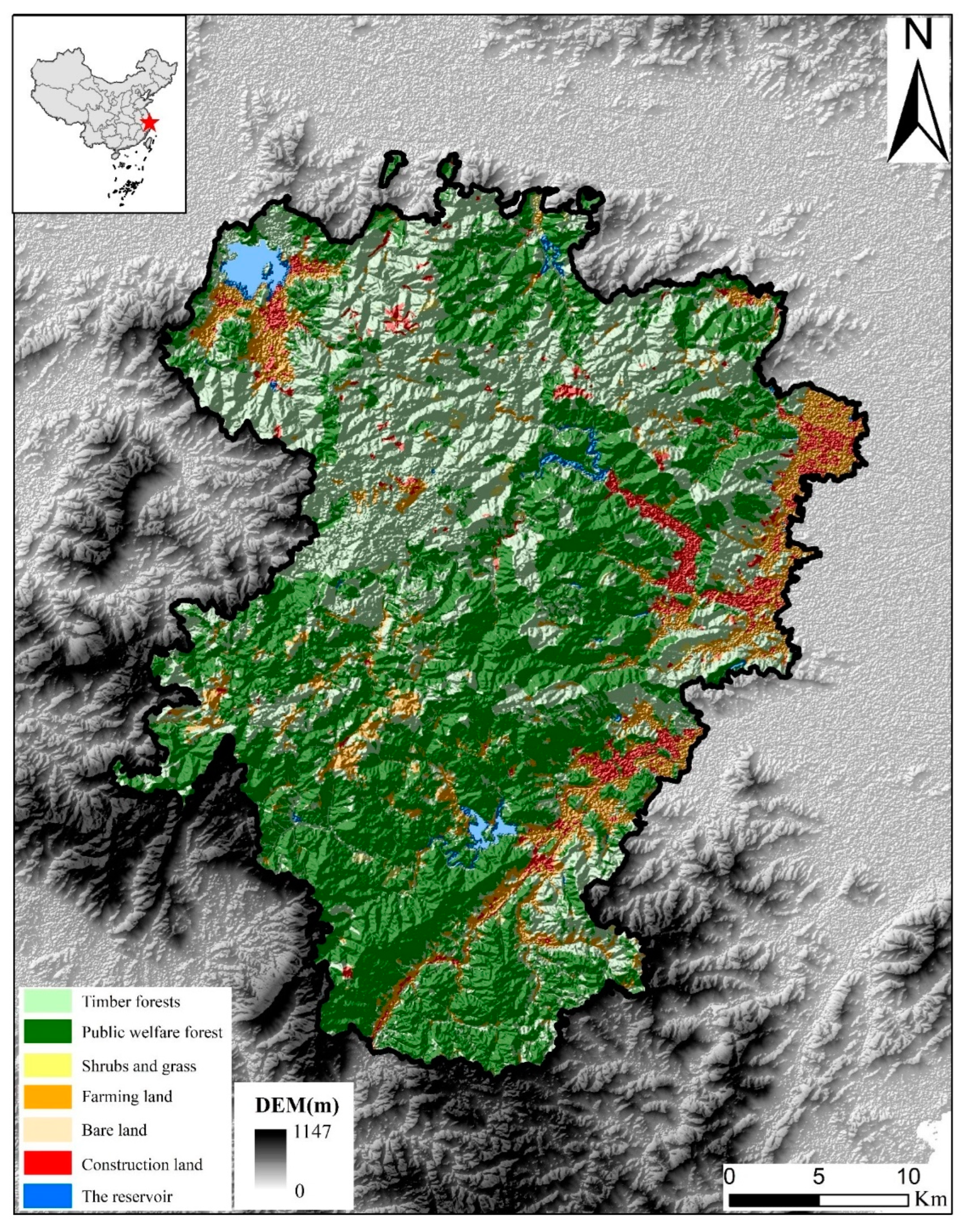
From the perspective of ecosystem structure-function-habitat, we chose three categories of indicators to develop forest ecosystem recovery indicators with ecological implications. Tree height, canopy closure, and community structure are classic indicators of forest structure. AGB is chosen as a functional indicator. The naturalness represents the habitat of the forest ecosystem. We also calculated NBR which is the major spectural indicator of the LandTrendr algorithm. The hybrid approach integrates the forest inventory, LiDAR, and Landsat data.
The main goal of the hybrid approach was the precise estimation of forest ecosystem recovery, especially in the middle restorative forest period. Therefore, firstly, 6 indicators were selected to construct the multiple estimation model after the references search. The weights of the indicators were calculated through the Analytic Hierarchy Process (AHP) and Entropy Weight Method (EWM), which combined the subjective and objective weights assignment methods. Secondly, we used visual interpretation and Google Earth images to evaluate the performance of the model. Then, a biodiversity index representing the resilience of forest ecosystem was constructed to verify its relationship with the output of the hybrid model. Thirdly, since the application of the hybrid approach was limited by the data availability, we used the RF algorithm to build the relationship between hybrid method results and the 12 independent variables, which could be applied in the time series results. Finally, we applied the hybrid model in the subtropical forest region to help local forests to facilitate temporal and spatial refinement management (Figure 1).

2.1. Study Area

Siming Mountain is located in eastern China (29°32′–29°59′N, 121°0′–121°25′E). Elevation ranges from 10 to 976 m with a mean slope of 19°. The mean annual temperature is 11.8 °C and annual rainfall is 1970 mm. With a humid subtropical monsoon climate, Siming Mountain is covered with subtropical evergreen broadleaf forests, most of which are secondary forests (Figure 2). Most primary forests were altered into other forest types such as spruce-fir mixed coniferous forests. Typical tree species distribute unevenly, including Pinus massoniana, Cunninghamia lanceolata, Schima superba, and Cyclobalanopsis jenseniana.
Siming Mountain is the drinking water source of Ningbo city and plays an important role in water conservation. Between 2010 and 2013, residents made huge profits from cultivating ornamental tree seedlings. Driven by the profit, many tea gardens, bamboo plantations, and broadleaf forests were replaced by seedling cultivation fields, which caught forest managers’ attention. Seedlings are sold with a soil ball to prevent dehydration during transportation. This practice results in the stripping away of a substantial amount of topsoil, leading to the loss of both nutrients and water conservation. Furthermore, the excessive use of chemical fertilizers and pesticides without proper scientific management in seedling cultivation results in water pollution. Therefore, seedling planting led to the loss of forest cover and ecosystem services. To achieve sustainable development that balanced the need for environmental protection with economic benefits, in 2013, the Ningbo city government invested 110 million RMB to restore 2266 ha of forest.

2.2. Multi-Source Spatial Database Development

The first type of data was field observation data. LFMI, which is the detailed and accurate full-cover inventory, was conducted every 10 years (e.g., 2005 and 2015). With the basic unit of the forest patch, the Ministry of Forestry of China issued a document that included comprehensive and detailed regulations on the conditions for the division of forest patches, survey content and methods, and the quality control procedures. LFMI data was obtained by field observations, including graphical data and the corresponding attribute database. The attribute database provided data on stands, tree height, diameter at breast height (DBH), canopy closure, tree age, naturalness, community structure, tree number per ha, main tree species, understory height, understory coverage, and other factors. The sampling accuracy was within 90% [38]. In terms of mean DBH, tree height, number of trees, and patch area, the AGB was calculated through biomass allometric equations (Figure S1). Please find the equation information in Table S1. The 242 trees with similar DBH were collected, harvested, and weighed separately for each organ to obtain biomass to construct the allometric equation (AGB = (0.079 × DBH2 × Height)0.9164) [39].
The second type of data was the passive remote sensing data, mainly Landsat images, which were pre-processed by the Google Earth Engine platform. The Landsat images were from June, 20th, to September, 20th in each year during 2000 to 2021. 107 images were collected to calculate spectral parameters (e.g., NBR).
The third type of data was the active remote sensing data. The LiDAR data, which penetrates vegetation to obtain three-dimensional information on the ground surface and forest canopy, is an important technical tool for the accurate extraction of topography and forest canopy height. The data was collected from March to April 2015, with a point density of 4 pts/m2 and spatial resolution of 0.2 m. The aircraft is Y-12 with the flight altitude of 3000 m, the flight speed of 240 km/h, and scanning frequency of 340 kHz.
Finally, all data were converted to raster images with a resolution of 30 m using ArcGIS 10.2 and LiDAR 360. The images were uniformly adjusted to the WGS1984 coordinate system and entered the multi-source vertical database.

2.3. The Multi-Source Hybrid Approach

2.3.1. Multi-Estimation Indicator System

Multi-source data were used to represent forest recovery. Firstly, we used 30 m grid to calculate the information entropy of all indicators (NBR, disturbance index, tree height, canopy closure, leaf area index, naturalness, type of community structure, above-ground biomass, and eluvial horizon thickness) in pre-experiments to select the appropriate indicators (Table S2). The information entropy measures the uncertainty of signals in information sources [40]. The lower the information entropy, the more information it can provide. Six indicators (NBR, tree height, canopy density, naturalness, community structure type, and above-ground biomass) with low information entropy were left from three types of data. Secondly, the AHP and EWM were used to calculate the weights of the indicators, respectively. The weights obtained by AHP and EWM, to a certain extent, overcame the disadvantages of the single weighting method alone. The arithmetic average of the two weight methods was calculated (Table 1). Lastly, the recovery value (RV) of the hybrid approach was calculated in terms of the multi-assessment indicator system.
Categorical and numerical indicators are used in forestry surveys to describe the state of the ecosystem. According to Forestry Survey Specification Manual, there are three grades of naturalness and community structure [41]. To quantify categorical indicators, we defined the correspondence between category and value (Table S3). For example, 0.165 for type III, 0.495 for type II and 0.83 for type I of naturalness.
The comprehensive recovery indicator of the hybrid approach was calculated after the standardization of all indicator values.
RV = j = 1 n Y j W cj
where RV is the comprehensive recovery indicator; Yj is the standardized value of the jth indicator; Wcj is the arithmetic averages of weights of AHP and EWM methods of the jth indicator.

2.3.2. Weights Calculation

AHP proposed by Saaty (2008) is a weight matrix system that can be used to determine the subjective weight of each indicator [42]. Local forestry experts compare all indicators in pairs in yaahp software to determine the relative importance. The EWM effectively avoids subjective interference in the weight-setting process and makes the results relatively objective [43].
(1) Standardization of indicators: the positive and negative indicators should be identified.
y ij = x x min x max x min               f o r   p o s i t i v e   i n d i c a t o r s x max x x max x min               f o r   n e g a t i v e   i n d i c a t o r s
where yij is the normalized value and x is the original value. xmax and xmin mean the maximum and minimum values of the indicators respectively.
(2) Indicator weights were calculated as the following equation.
H j = i = 1 n Y ij ln Y ij ln n
Y ij = y ij i = 1 n y ij
w ej = 1 H j j = 1 n 1 H j
where Hj is the information entropy value.

2.4. Performance Assessment

Since it was difficult to identify the spatial pattern of the restored area with the 30 m resolution map, in order to obtain a better display the recovered values in each pixel were smoothed into 300 m spatial resolution hexagonal pixels. The hexagonal pixel value represented the mean value of the region. Next, since the LiDAR data and LFMI data were acquired in 2015, we presented historical images from Google Earth (25 cm resolution) in 2015 to illustrate the 15 regions with the greatest differences. The RV and RF results of 3722 pixels (30 m) were used for visual interpretation based on historical Google Earth imagery to build the confusion matrix (CM) for assessing the accuracy of the approaches. The CM visualizes and summarizes the performance of the classification algorithm [44]. The column in the matrix represents the true recovery information, where the value is the pixel number. The producer’s accuracy (PA), user’s accuracy (UA), overall accuracy (OA), and Kappa coefficient were calculated from the confusion matrix.
PA is the number of reference sites classified accurately divided by the total number of reference sites for that class.
PA = X ij X + i
where X ij is the number in row i and column j; X + i is the sum of the column i.
UA is the proportion of the number of correctly classified pixels for a particular class of total pixels in that class.
UA = X ij X i +
where X ij is the number in row i and column j; Xi+ is the sum of the row i.
Overall Accuracy (OA) is the ratio of the total number of correctly classified pixels to the total number of pixels.
OA = i = 1 n X ij N
where n is the number of rows or columns; X ij is the number in row i and column j; and N is the sum of all pixels. The Kappa coefficient is another overall measure of the accuracy of a classification product. It separates the “chance” and “certain” factors and evaluates whether the classification is better than a random classification or not. The negative value indicates a worse classification than random classification. The positive value around 1 indicates a significantly better classification than random classification.
Kappa = N i = 1 n X ij i = 1 n X i + X + i N 2 i = 1 n X i + X + i
P 0 = i = 1 n x ii N
P e = i = 1 n x i + x + i N 2
where P0 is OA. Pe indicates the proportion of pixels that are correctly classified by chance. Xi+ is the sum of all numbers in the row i. N is the total number of pixels.
In addition, the biodiversity recovery value (BRV) was set to represent forest ecosystem resilience. Tree and shrub species richness, as indicators to characterize forest biodiversity, reflect the level of forest ecological functions [45]. Therefore, the number of tree species, the understory height, and the understory coverage from LFMI data were used for calculating BRV.
BRV = 1 3 y j 3
where BRV is biodiversity recovery value; yj is the standardized value of the jth indicator. The weight of the three indicators is set to one third.

2.5. Forest Ecological Recovery Assessment Model Based on RF

Random forest, which has excellent computational speed and reliable results, generates multiple decision trees using randomly selected training samples and output the variable importance [46,47]. Moreover, the RF also has good application results in predicting forest recovery [48]. In the pre-experiment, 23 spectral indices were selected as the independent variables of the RF method. We excluded indices with low importance values (e.g., blue, TCB, swir1, SAVI, TCD, NBR, DVI, nir, PVI, and green). The 12 indices with high importance were selected as the independent variable for the actual input of the RF (Table 2). ArcGIS Pro 2.8.0 was used with default parameters. Based on raster data of the year 2015, 50% of the pixels were randomly selected as training data and the remaining 50% were used as validation data. The model performance was assessed using the coefficient of determination (R2) and root mean square error (RMSE) metrics [49].

2.6. The Forest Refines Management Application of the Hybrid Approach

Detecting abnormal disturbant areas and calculating the rate of forest recovery in different areas helps maximize the benefits of local stakeholders in the forest recovery process. It helps (relevant authorities) achieve scientific forest management and efficient use of forest resources [6]. To obtain the annual area of forest loss, we used the LandTrendr algorithm to locate the annual area of deforestation and then subtracted the annual area of forest recovery from the hybrid approach. By comparing the areas of forest loss every year, we detected the time and location of the abnormal deforestation. The recovery rate of the pixels in a given year was calculated by subtracting the recovery values of the previous year. Finally, local spatial statistics (e.g., local Getis Gi* for hot and cold spot detection) were used to determine where the long-term spectral recovery rate was significantly slower than that of other regions.
The recovery duration of ecological functions of individual pixels was estimated through the space-for-time substitution method. The age of the trees recorded in the LFMI data, which was used as the number of recovery years on the site, was the independent variable. We used a variety of equations to fit the data in advance, and the logistic equation reflected the optimal coefficient of determination (R2). The mean value of the hybrid approach with the same recovery years was the dependent variable of the logistic equation. The logistic equation was fitted to predict the distribution of forest recovery value in Siming Mountain from 2022 to 2050, assuming that areas with similar forestry policy will not be disturbed by deforestation. To estimate the minimum time for forest ecological recovery to reach a steady state at the regional scale, the one-way ANOVA test was used in different years. We hypothesized that the year could be used as the end of the forest control policy when RV values didn’t show a significant difference compared to the RV values in the subsequent years at 0.05 significance level. Please find the flowchart (Figure S2) to help understand this process.

3. Result

3.1. The Performance of the Hybrid Approach

3.1.1. Forest Recovery Mapping

The regions could be classified based on RV. Regions with RV less than 0.33, including regions A to E, exhibited a lack of vegetation cover or are characterized by seasonal crops. Regions with RV greater than or equal to 0.33 but less than 0.66, including regions F to J, were classified as middle restorative forest, and displayed moderate vegetation cover as well as significant human disturbance. On the other hand, areas with RV greater than or equal to 0.66 were classified into restored forest, specifically regions K to O, exhibiting trees greater than 2.6 m in height and canopy density greater than 0.32 in terms of LFMI, with three vegetation layers and minimal human disturbance (Figure 3). The results showed that the hybrid approach well identify the recovery process of the forests well.

3.1.2. Accuracy Assessment Based on Visual Interpretation

The results of the CM showed that the OA of the hybrid approach was 0.94. The PAs of the three recovery stages of the hybrid approach achieved at least 0.93. The hybrid approach has high UA in the initial restorative and restored forest areas. The hybrid approach was accurate in identifying initial restorative, middle restorative, and restored forest stages of recovery (Table 3). The accuracy of RF was lower performance than the hybrid approach.

3.1.3. The Relationship between RV and Biodiversity Index

The determination coefficient of the fitting equations of RV and BRV is 0.57. The RV increased with the BRV increased. The pixels with the RV around 0.25 and 0.75 were more aggregated along the 1:1 line than those with RV around 0.50 (Figure 4).

3.2. The RF Correction Model Performance

The tree age (Importance value (IV) = 0.67) was the key variable in improving the prediction accuracy of the RF model, followed by slope degree (IV = 0.05), SR (IV = 0.05), and NDVI (IV = 0.05). The order of the other variables was DI (IV = 0.01) and TCA (IV = 0.01) < swir2 (IV = 0.02), TCW (IV = 0.02), and TCG (IV = 0.02) < BI (IV = 0.03) and Red (IV = 0.03) < Elevation (IV = 0.04). The R2 and RMSE of the RF model were 0.78 and 0.14, respectively (Figure 5). The UA of RF is greater than 0.90 in the recovery value range of (0–0.33] and (0.66–1.67] (Table 3).

3.3. The Application of the Hybrid Approach

3.3.1. Spatio-Temporal Refinement Management Applications

The hybrid approach result could be used to identify the regional abnormal disturbance of human activities (Table 4). The result showed that the area of disturbance in the study area was almost lower than 200 ha per year from 2001 to 2009. The area of disturbance grew significantly from 2009 to 2012 and reached the highest value in 2011 (460.17 ha) and 2012 (411.00 ha). From 2013 to 2018, the disturbance area was significantly reduced. After 2019, the area of disturbance gradually rebounded, although it did not exceed 200 ha.
We demonstrated the cold spots for recovery rate from 2001 to 2020 (Figure 6). The results showed the cold spot cluster of forest recovery in the southern part of Siming Mountain, which was the public welfare forest. The mean elevation of this area was 723 m, much higher than the average elevation of 338 m in the study area. The mean slope degree was 41°, higher than the mean value of 19°. The thickness of the soil A layer, which was divided into thick (>80 cm), medium (40–79 cm), and thin (<40 cm) classes, was all less than 40 cm.

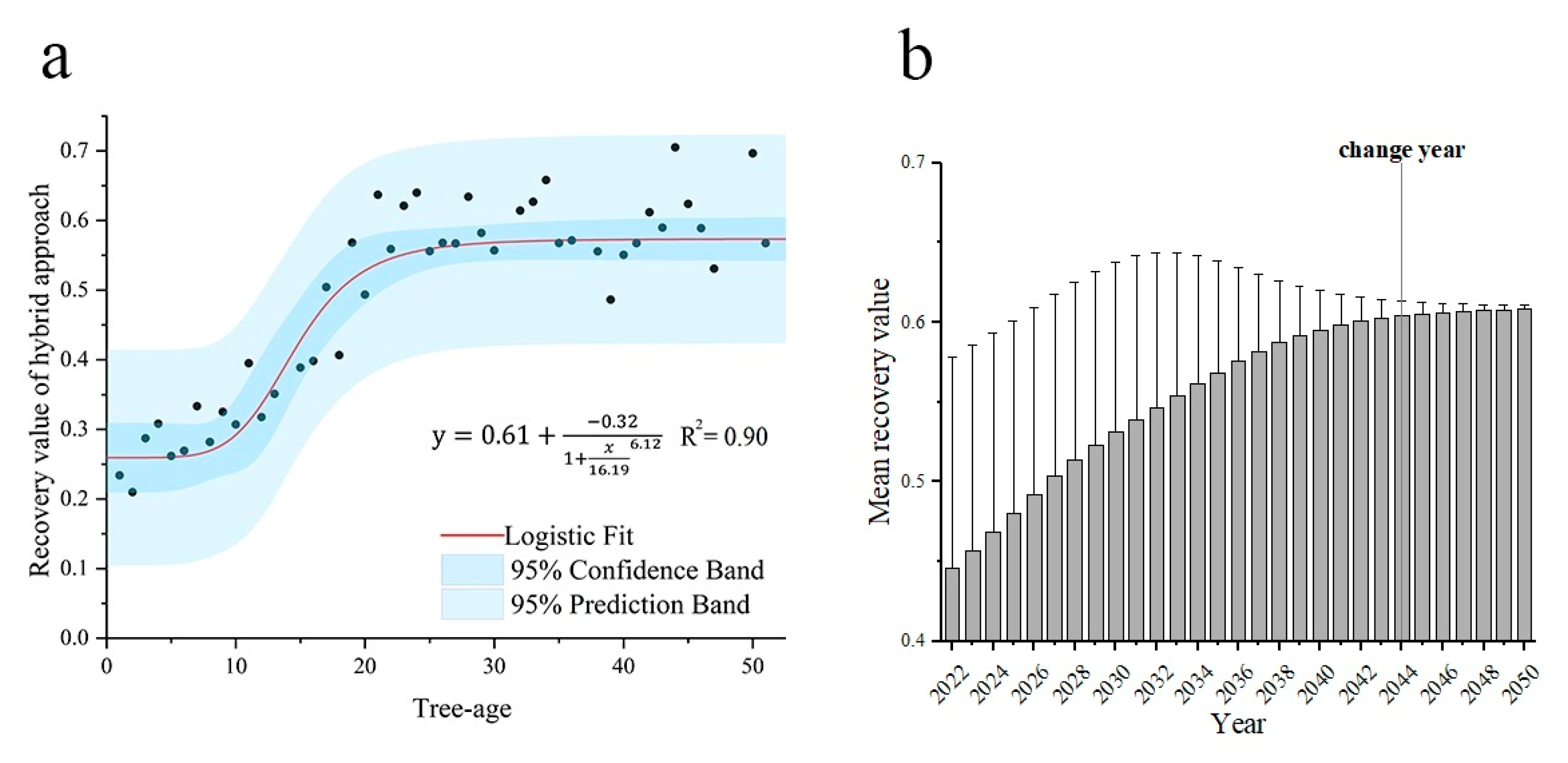
3.3.2. Temporal Refinement Applications

The hybrid approach result could help design the deadline of the strict policy. R2 of the space-for-time substitution logistic equation (Figure 7a) was 0.90. The logistic curve represented three different stages of forest recovery. The first stage was from 0 to 10 years, which could be called the preparation period. During this period, the recovery was relatively stable. The second stage was from 10 to 20 years. This was the critical period of forest recovery, which was the fastest. The third stage was from 20 to 50 years, when the forest recovery gradually stabilized. We used the logistic equation to predict the recovery situation after 2022 (Figure 7b). The result showed that under the ideal situation without the disturbances or extreme weather, the study area would continue to recover significantly from 2022 to 2044 but start to recover insignificantly after 2045 and become stable. It suggested that the government could possibly adjust the strict policy in 2044.

4. Discussion

4.1. The Hybrid Model Accuracy

Our results showed that multi-source data and the recovery value of the hybrid method were able to provide reliable refined temporal and spatial information on the recovery of forest ecology in the pixel and regional scales. In general, scholars proposed considering both the multispectral metrics of the post-disturbance and spatial structural characteristics for improving the forest recovery detection accuracy [24,58,59]. The hybrid method was constructed based on the structure–function–habitat three aspects which reflected the ecological meaning and overcame the disadvantage of the fast recovery rate of the spectral index. High-resolution historical imagery from Google Earth can be used to verify the state of forest restoration [60]. Our validation results showed that the hybrid approach was accurate in detecting forest recovery. Shrub species richness and tree species richness are often selected as indicators to characterize forest biodiversity [45]. This is because areas with more tree species tend to have higher levels of ecosystem services [61,62]. For example, scholars found that tree species richness showed a positive hump-shaped relationship with multiple ecosystem services (e.g., production of biomass, soil carbon storage, berry production, and game production potential) [61]. Moreover, shrub species play an important role in providing ecosystem function, especially in arid sand dune ecosystems [63]. The index consists of the number of tree species and the number of shrubs and herbs, and increases with the increase in the RV value constructed by the hybrid model. This means that the hybrid model based on structure–function–habitat also has the ability to characterize the biodiversity of forest ecosystems. Therefore, the hybrid model brings new ideas to sustainable forest management.

4.2. Implications of Assessment Results

This study proposed a comprehensive RV index that reflects the forest ecosystem function by selecting ecological indicators. The index could accurately distinguish the recovery of initial restorative forest, middle restorative forest, and forest. It also has a wide range of ecological implications. By comparing the LFMI data from 2005 and 2015, residents preferred to convert the tea gardens, bamboo forests, and even the forest into the land used for seedling plantations. This expansion of the seedling industry led to an unusual trend of deforestation. Since the local forestry administration launched a strict no-deforestation policy in 2013, the disturbed area of forests in Siming Mountain decreased significantly from 2013 to 2018. Therefore, the RV index addressed the major problem for forestry management in Siming Mountain, which was the detection of vegetation changes resulting from the expansion of the seedling cultivation fields. There were three main policies for controlling the expansion of seedling cultivation fields. The first policy one was to prohibit the planting of seedlings in forested areas with a slope degree larger than 25 degrees and a soil thickness of less than 30 cm. The second policy was to clear seedling cultivation fields in public welfare forests. The third policy was to carry out forest ecological recovery projects in disturbed areas between 2013 and 2018. The comprehensive RV index proposed in this study could identify and assess in a timely manner whether seedling cultivation fields had been converted to woodlands with the policy requirements through annual monitoring of the disturbance area. It also guided the managers to prevent the rebound of seedling cultivation field expansion. At the same time, it could discover the regions with slow recovery rates and causal factors. The results provided scientific support for the managers to carry out ecological recovery projects.
The result of the hybrid approach solved the local forest management problem by estimating the restorative process of the disturbed forest. It helped to scientifically determine the policy implementation period. In forest recovery, it takes a long time to recover the ecological functions with a stable and redundant structure and community for achieving a high resilience ability. The results can provide managers with a reasonable assessment of the economic pressures and benefits associated with recovery. The solution to this problem was crucial, because the key components that determine forest restoration include the social context and economic pressure, in addition to ensuring the tree survival rate and controlling the factors that disturbed forests [64]. Since the study area Siming Mountain involved one municipal and four district forest management agencies, it was not sufficient for local managers to know only about the forest recovery condition in their own areas. The ecosystem services of interest varied from region to region. Assessing the distribution and recovery of forest ecosystem functions in the whole region facilitates a better allocation of different resources. The focus on the ecological integrity of the forest at the landscape level ensured the different forest ecosystem service functions (e.g., water conservation).

4.3. Strengths and Limitations

The advantage of the hybrid approach was the continuous monitoring of the changes in forest ecological functions in the large region with relatively low cost and human input. Large-scale regional studies might not always have access to LiDAR and LFMI data. In such cases, the random forest algorithm can be used to fit RV values by supplementing NBR values and tree age to obtain the recovery assessment for years without LiDAR and LFMI data. We comprehensively used the advantages of various data sources including the long-term and large-area data availability of Landsat, the comprehensiveness of forest resource survey data content, and the high accuracy of Lidar data on forest structure parameter detection. Furthermore, the results met the requirements of the forest management department for spatio-temporal refinement management, including the detection of historical areas of disturbances, the discovery of forest recovery rate, and the length of time that the forest returned to the stable state.
The selection of indicators for the hybrid approach can be further improved by the indices that reflect the functionality of the forest in detail, such as plant area density and “plant” area index [65]. When we estimated the length of the recovery time in the study area, the influences of the climate (e.g., drought) and the artificial management practices were not considered. The research showed that the forest recovery would slow down 1–3 years after the drought in China, especially the artificial forest recovered faster than the natural forest [66]. However, the study suggested that although the management practices contributed to the recovery of forest structure in a temperate forest, forest still recovered well from disturbances without human intervention [67].

5. Conclusions

Accurately assessing forest ecosystem recovery in a large region required the integration of data from multiple sources. Integrating indicators of forest structure and function, besides spectral indicators, significantly improved the accuracy of forest recovery assessments. The naturalness and community structure data from LFMI, tree height, and canopy density data from LiDAR provided information on the structure, function, and habitat of the forest. The visual interpretation of Google Earth imagery showed that the hybrid approach was able to accurately distinguish different stages of restoration. The biodiversity index constructed using the number of tree species and shrub and herbaceous coverage as information sources increased with the increase in the hybrid approach results. It showed that the hybrid model could evaluate forest restoration from the aspect of the ecological function of the forest ecosystem.
The tree age was the most crucial factor contributing to the hybrid approach assessment results through the RF model. From the perspective of the application of spatio-temporal-refined management, the hybrid approach made it possible to detect the annual loss of forest area due to the expansion of the seedling fields. Moreover, the spatial and temporal distribution of forest recovery rates provided the basis for detecting areas with slow recovery rates and improving the efficiency of ecological recovery projects in conjunction with recovery goals. The space-for-time substitution approach was used to build the predictive model by fitting the recovery values calculated from the hybrid approach and the age of trees through the logistic equation. The model predicted the time it would take for forests to recover to a stable state and provided the scientific data support for the design of the duration time required to implement ecological restoration policies.

Supplementary Materials

The following supporting information can be downloaded at: https://www.mdpi.com/article/10.3390/rs15102667/s1, Figure S1. Aboveground biomass distribution of the study area in 2005 and 2015; Figure S2. A flowchart of how to find the key year x. We define that the recovery of the study area will reach a stable state after x [68]; Table S1. Table of key information about the plots; Table S2. Alternative parameters and information entropy; Table S3. Table of definitions of naturalness and community structure type values.

Author Contributions

Conceptualization, M.L., S.Z. and Y.R.; Data curation, X.Z., W.W. and K.C.; Funding acquisition, Y.R.; Methodology, M.L.; Software, M.L.; Validation, Y.S.; Writing—original draft, M.L. and S.Z.; Writing—review & editing, S.Z. All authors have read and agreed to the published version of the manuscript.

Funding

This work was supported by National Key Research Program of China (2022YFF1303001), National Natural Science Foundation of China (42001210, 31972951, 31670645, 42171100, 41801182, and 41807502), National Social Science Fund (17ZDA058), Fujian Provincial Department of S&T Project (2022T3047, 2021I0041, 2021T3058, 2019J01136), the Strategic Priority Research Program of the Chinese Academy of Sciences (XDA23020502), Xiamen S&T Project (3502Z20226016). We are grateful to the anonymous reviewers for their constructive suggestions.

Data Availability Statement

The data presented in this study are available on request from the corresponding author.

Acknowledgments

Thanks to the Ningbo Natural Resources Planning Bureau for collecting and providing the high quality LFMI data and LiDAR data required for the study.

Conflicts of Interest

The authors declare that they have no known competing financial interests or personal relationships that could have influenced the work reported in this paper.

References

  1. Seidl, R.; Thom, D.; Kautz, M.; Martin-Benito, D.; Peltoniemi, M.; Vacchiano, G.; Wild, J.; Ascoli, D.; Petr, M.; Honkaniemi, J.; et al. Forest disturbances under climate change. Nat. Clim. Chang. 2017, 7, 395–402. [Google Scholar] [CrossRef]
  2. Hansen, M.C.; Potapov, P.V.; Moore, R.; Hancher, M.; Turubanova, S.A.; Tyukavina, A.; Thau, D.; Stehman, S.V.; Goetz, S.J.; Loveland, T.R. High-resolution global maps of 21st-century forest cover change. Science 2013, 342, 850–853. [Google Scholar] [CrossRef] [PubMed]
  3. National Greening Committee of China. Outline of the National Land Greening Plan (2022–2030). Available online: http://www.forestry.gov.cn/main/586/20220910/120737578312352.html (accessed on 10 September 2022).
  4. Oliver, T.H.; Heard, M.S.; Isaac, N.J.B.; Roy, D.B.; Procter, D.; Eigenbrod, F.; Freckleton, R.; Hector, A.; Orme, C.D.L.; Petchey, O.L.; et al. Biodiversity and Resilience of Ecosystem Functions. Trends Ecol. Evol. 2015, 30, 673–684. [Google Scholar] [CrossRef] [PubMed]
  5. Lamb, D.; Stanturf, J.; Madsen, P. Palle Madsen What is forest landscape restoration? For. Landsc. Restor. 2012, 15, 3–23. [Google Scholar] [CrossRef]
  6. Stanturf, J.A.; Palik, B.J.; Dumroese, R.K. Contemporary forest restoration: A review emphasizing function. For. Ecol. Manag. 2014, 331, 292–323. [Google Scholar] [CrossRef]
  7. Castro, J.; Morales-Rueda, F.; Navarro, F.B.; Lof, M.; Vacchiano, G.; Alcaraz-Segura, D. Precision restoration: A necessary approach to foster forest recovery in the 21st century. Restor. Ecol. 2021, 29, e13421. [Google Scholar] [CrossRef]
  8. Smith, W.B. Forest inventory and analysis: A national inventory and monitoring program. Environ. Pollut. 2002, 116, S233–S242. [Google Scholar] [CrossRef]
  9. Lechner, A.M.; Foody, G.M.; Boyd, D.S. Applications in Remote Sensing to Forest Ecology and Management. One Earth 2020, 2, 405–412. [Google Scholar] [CrossRef]
  10. Frolking, S.; Palace, M.W.; Clark, D.B.; Chambers, J.Q.; Shugart, H.H.; Hurtt, G.C. Forest disturbance and recovery: A general review in the context of spaceborne remote sensing of impacts on aboveground biomass and canopy structure. J. Geophys. Res.-Biogeosci. 2009, 114, G00E02. [Google Scholar] [CrossRef]
  11. Camarretta, N.; Harrison, P.A.; Bailey, T.; Potts, B.; Lucieer, A.; Davidson, N.; Hunt, M. Monitoring forest structure to guide adaptive management of forest restoration: A review of remote sensing approaches. New For. 2020, 51, 573–596. [Google Scholar] [CrossRef]
  12. Vancutsem, C.; Achard, F.; Pekel, J.F.; Vieilledent, G.; Carboni, S.; Simonetti, D.; Gallego, J.; Aragao, L.E.O.C.; Nasi, R. Long-term (1990–2019) monitoring of forest cover changes in the humid tropics. Sci. Adv. 2021, 7, eabe1603. [Google Scholar] [CrossRef] [PubMed]
  13. Masek, J.G.; Huang, C.; Wolfe, R.; Cohen, W.; Hall, F.; Kutler, J.; Nelson, P. North American forest disturbance mapped from a decadal Landsat record. Remote Sens. Environ. 2008, 112, 2914–2926. [Google Scholar] [CrossRef]
  14. Kennedy, R.E.; Cohen, W.B.; Schroeder, T.A. Trajectory-based change detection for automated characterization of forest disturbance dynamics. Remote Sens. Environ. 2007, 110, 370–386. [Google Scholar] [CrossRef]
  15. Zhu, Z.; Fu, Y.; Woodcock, C.E.; Olofsson, P.; Vogelmann, J.E.; Holden, C.; Wang, M.; Dai, S.; Yu, Y. Including land cover change in analysis of greenness trends using all available Landsat 5, 7, and 8 images: A case study from Guangzhou, China (2000-2014). Remote Sens. Environ. 2016, 185, 243–257. [Google Scholar] [CrossRef]
  16. Vogelmann, J.E.; Gallant, A.L.; Shi, H.; Zhu, Z. Perspectives on monitoring gradual change across the continuity of Landsat sensors using time-series data. Remote Sens. Environ. 2016, 185, 258–270. [Google Scholar] [CrossRef]
  17. Ahmed, O.S.; Franklin, S.E.; Wulder, M.A. Interpretation of forest disturbance using a time series of Landsat imagery and canopy structure from airborne lidar. Can. J. Remote Sens. 2014, 39, 521–542. [Google Scholar] [CrossRef]
  18. Knudby, A.; Newman, C.; Shaghude, Y.; Muhando, C. Simple and effective monitoring of historic changes in nearshore environments using the free archive of Landsat imagery. Int. J. Appl. Earth Obs. Geoinf. 2010, 12, S116–S122. [Google Scholar] [CrossRef]
  19. Kennedy, R.E.; Yang, Z.; Cohen, W.B. Detecting trends in forest disturbance and recovery using yearly Landsat time series: 1. LandTrendr—Temporal segmentation algorithms. Remote Sens. Environ. 2010, 114, 2897–2910. [Google Scholar] [CrossRef]
  20. Bullock, E.L.; Woodcock, C.E.; Souza, C., Jr.; Olofsson, P. Satellite-based estimates reveal widespread forest degradation in the Amazon. Glob. Chang. Biol. 2020, 26, 2956–2969. [Google Scholar] [CrossRef]
  21. Kennedy, R.E.; Yang, Z.; Gorelick, N.; Braaten, J.; Cavalcante, L.; Cohen, W.B.; Healey, S. Implementation of the LandTrendr Algorithm on Google Earth Engine. Remote Sens. 2018, 10, 691. [Google Scholar] [CrossRef]
  22. Wang, Y.; Ziv, G.; Adami, M.; Mitchard, E.; Batterman, S.A.; Buermann, W.; Marimon, B.S.; Marimon Junior, B.H.; Reis, S.M.; Rodrigues, D.; et al. Mapping tropical disturbed forests using multi-decadal 30 m optical satellite imagery. Remote Sens. Environ. 2019, 221, 474–488. [Google Scholar] [CrossRef]
  23. Reygadas, Y.; Spera, S.; Galati, V.; Salisbury, D.S.; Silva, S.; Novoa, S. Mapping forest disturbances across the Southwestern Amazon: Tradeoffs between open-source, Landsat-based algorithms. Environ. Res. Commun. 2021, 3, 091001. [Google Scholar] [CrossRef]
  24. Meng, Y.; Liu, X.; Wang, Z.; Ding, C.; Zhu, L. How can spatial structural metrics improve the accuracy of forest disturbance and recovery detection using dense Landsat time series? Ecol. Indic. 2021, 132, 108336. [Google Scholar] [CrossRef]
  25. Bolton, D.K.; Coops, N.C.; Wulder, M.A. Characterizing residual structure and forest recovery following high-severity fire in the western boreal of Canada using Landsat time-series and airborne lidar data. Remote Sens. Environ. 2015, 163, 48–60. [Google Scholar] [CrossRef]
  26. Scheffer, M.; Carpenter, S.R.; Dakos, V.; van Nes, E.H. Generic Indicators of Ecological Resilience: Inferring the Chance of a Critical Transition. Annu. Rev. Ecol. Evol. Syst. 2015, 46, 145–167. [Google Scholar] [CrossRef]
  27. Oettel, J.; Lapin, K. Linking forest management and biodiversity indicators to strengthen sustainable forest management in Europe. Ecol. Indic. 2021, 122, 107275. [Google Scholar] [CrossRef]
  28. Dobor, L.; Hlasny, T.; Rammer, W.; Barka, I.; Trombik, J.; Pavlenda, P.; Seben, V.; Stepanek, P.; Seidl, R. Post-disturbance recovery of forest carbon in a temperate forest landscape under climate change. Agric. For. Meteorol. 2018, 263, 308–322. [Google Scholar] [CrossRef]
  29. McLachlan, S.M.; Bazely, D.R. Recovery patterns of understory herbs and their use as indicators of deciduous forest regeneration. Conserv. Biol. 2001, 15, 98–110. [Google Scholar] [CrossRef]
  30. Bartels, S.F.; Chen, H.Y.H.; Wulder, M.A.; White, J.C. Trends in post-disturbance recovery rates of Canada’s forests following wildfire and harvest. For. Ecol. Manag. 2016, 361, 194–207. [Google Scholar] [CrossRef]
  31. Sankey, T.; Donager, J.; McVay, J.; Sankey, J.B. UAV lidar and hyperspectral fusion for forest monitoring in the southwestern USA. Remote Sens. Environ. 2017, 195, 30–43. [Google Scholar] [CrossRef]
  32. Johnson, K.D.; Birdsey, R.; Cole, J.; Swatantran, A.; O’Neil-Dunne, J.; Dubayah, R.; Lister, A. Integrating LIDAR and forest inventories to fill the trees outside forests data gap. Environ. Monit. Assess. 2015, 187, 623. [Google Scholar] [CrossRef]
  33. Kennedy, R.E.; Yang, Z.; Cohen, W.B.; Pfaff, E.; Braaten, J.; Nelson, P. Spatial and temporal patterns of forest disturbance and regrowth within the area of the Northwest Forest Plan. Remote Sens. Environ. 2012, 122, 117–133. [Google Scholar] [CrossRef]
  34. de Avila, A.L.; van der Sande, M.T.; Dormann, C.F.; Pena-Claros, M.; Poorter, L.; Mazzei, L.; Ruschel, A.R.; Silva, J.N.M.; de Carvalho, J.O.P.; Bauhus, J. Disturbance intensity is a stronger driver of biomass recovery than remaining tree-community attributes in a managed Amazonian forest. J. Appl. Ecol. 2018, 55, 1647–1657. [Google Scholar] [CrossRef]
  35. Do, H.T.T.; Grant, J.C.; Ngoc Bon, T.; Zimmer, H.C.; Lam Dong, T.; Nichols, J.D. Recovery of tropical moist deciduous dipterocarp forest in Southern Vietnam. For. Ecol. Manag. 2019, 433, 184–204. [Google Scholar] [CrossRef]
  36. Villa, P.M.; Martins, S.V.; de Oliveira Neto, S.N.; Rodrigues, A.C.; Hissa Safar, N.V.; Monsanto, L.D.; Cancio, N.M.; Ali, A. Woody species diversity as an indicator of the forest recovery after shifting cultivation disturbance in the northern Amazon. Ecol. Indic. 2018, 95, 687–694. [Google Scholar] [CrossRef]
  37. Spasojevic, M.J.; Bahlai, C.A.; Bradley, B.A.; Butterfield, B.J.; Tuanmu, M.-N.; Sistla, S.; Wiederholt, R.; Suding, K.N. Scaling up the diversity-resilience relationship with traitdatabases and remote sensing data: The recovery ofproductivity after wildfire. Glob. Chang. Biol. 2016, 22, 1421–1432. [Google Scholar] [CrossRef] [PubMed]
  38. Ren, Y.; Deng, L.-Y.; Zuo, S.-D.; Song, X.-D.; Liao, Y.-L.; Xu, C.-D.; Chen, Q.; Hua, L.-Z.; Li, Z.-W. Quantifying the influences of various ecological factors on land surface temperature of urban forests. Environ. Pollut. 2016, 216, 519–529. [Google Scholar] [CrossRef] [PubMed]
  39. Zuo, S.-D.; Ren, Y.; Weng, X.; Ding, H.; Luo, Y. Biomass allometric equations of nine common tree species in an evergreen broadleaved forestof subtropical China. Chin. J. Appl. Ecol. 2015, 26, 356–362. [Google Scholar] [CrossRef]
  40. Chen, C.-H. A Novel Multi-Criteria Decision-Making Model for Building Material Supplier Selection Based on Entropy-AHP Weighted TOPSIS. Entropy 2020, 22, 259. [Google Scholar] [CrossRef]
  41. Meng, Y.; Cao, B.; Dong, C.; Dong, X. Mount Taishan forest ecosystem health assessment based on forest inventory data. Forests 2019, 10, 657. [Google Scholar] [CrossRef]
  42. Saaty, T.L. Relative Measurement and Its Generalization in Decision Making Why Pairwise Comparisons are Central in Mathematics for the Measurement of Intangible Factors The Analytic Hierarchy/Network Process (To the Memory of my Beloved Friend Professor Sixto Rios Garcia). Rev. De La Real Acad. De Cienc. Exactas Fis. Y Nat. Ser. A-Mat. 2008, 102, 251–318. [Google Scholar] [CrossRef]
  43. Liu, L.; Zhou, J.; An, X.; Zhang, Y.; Yang, L. Using fuzzy theory and information entropy for water quality assessment in Three Gorges region, China. Expert Syst. Appl. 2010, 37, 2517–2521. [Google Scholar] [CrossRef]
  44. Wagle, N.; Acharya, T.D.; Kolluru, V.; Huang, H.; Lee, D.H. Multi-Temporal Land Cover Change Mapping Using Google Earth Engine and Ensemble Learning Methods. Appl. Sci. 2020, 10, 8083. [Google Scholar] [CrossRef]
  45. Torras, O.; Saura, S. Effects of silvicultural treatments on forest biodiversity indicators in the Mediterranean. For. Ecol. Manag. 2008, 255, 3322–3330. [Google Scholar] [CrossRef]
  46. Breiman, L. Random Forests. Mach. Learn. 2001, 45, 5–32. [Google Scholar] [CrossRef]
  47. Rodriguez-Galiano, V.F.; Ghimire, B.; Rogan, J.; Chica-Olmo, M.; Rigol-Sanchez, J.P. An assessment of the effectiveness of a random forest classifier for land-cover classification. Isprs J. Photogramm. Remote Sens. 2012, 67, 93–104. [Google Scholar] [CrossRef]
  48. Bright, B.C.; Hudak, A.T.; Kennedy, R.E.; Braaten, J.D.; Henareh Khalyani, A. Examining post-fire vegetation recovery with Landsat time series analysis in three western North American forest types. Fire Ecol. 2019, 15, 8. [Google Scholar] [CrossRef]
  49. Ahmed, O.S.; Franklin, S.E.; Wulder, M.A.; White, J.C. Characterizing stand-level forest canopy cover and height using Landsat time series, samples of airborne LiDAR, and the Random Forest algorithm. Isprs J. Photogramm. Remote Sens. 2015, 101, 89–101. [Google Scholar] [CrossRef]
  50. Powell, S.L.; Cohen, W.B.; Yang, Z.; Pierce, J.D.; Alberti, M. Quantification of impervious surface in the Snohomish Water Resources Inventory Area of Western Washington from 1972-2006. Remote Sens. Environ. 2008, 112, 1895–1908. [Google Scholar] [CrossRef]
  51. Pflugmacher, D.; Cohen, W.B.; Kennedy, R.E. Using Landsat-derived disturbance history (1972-2010) to predict current forest structure. Remote Sens. Environ. 2012, 122, 146–165. [Google Scholar] [CrossRef]
  52. Chen, C.; Bu, J.; Zhang, Y.; Zhuang, Y.; Chu, Y.; Hu, J.; Guo, B. The application of the tasseled cap transformation and feature knowledge for the extraction of coastline information from remote sensing images. Adv. Space Res. 2019, 64, 1780–1791. [Google Scholar] [CrossRef]
  53. Baig, M.H.A.; Zhang, L.; Shuai, T.; Tong, Q. Derivation of a tasselled cap transformation based on Landsat 8 at-satellite reflectance. Remote Sens. Lett. 2014, 5, 423–431. [Google Scholar] [CrossRef]
  54. Crist, E.P.; Cicone, R.C. A physically-based transformation of thematic mapper data—The TM tasseled cap. IEEE Trans. Geosci. Remote Sens. 1984, 22, 256–263. [Google Scholar] [CrossRef]
  55. Jordan, C.F. Derivation of leaf-area index from quality of light on forest floor. Ecology 1969, 50, 663–666. [Google Scholar] [CrossRef]
  56. Piao, S.; Mohammat, A.; Fang, J.; Cai, Q.; Feng, J. NDVI-based increase in growth of temperate grasslands and its responses to climate changes in China. Glob. Environ. Chang.-Hum. Policy Dimens. 2006, 16, 340–348. [Google Scholar] [CrossRef]
  57. Chen, W.H.; Liu, L.Y.; Zhang, C.; Wang, J.H.; Wang, J.D.; Pan, Y.C. Monitoring the seasonal bare soil areas in Beijing using multi-temporal TM images. In Proceedings of the IEEE International Geoscience and Remote Sensing Symposium, Anchorage, AK, 20–24 September 2004; IEEE: New York, NY, USA; pp. 3379–3382.
  58. White, J.C.; Wulder, M.A.; Hermosilla, T.; Coops, N.C.; Hobart, G.W. A nationwide annual characterization of 25 years of forest disturbance and recovery for Canada using Landsat time series. Remote Sens. Environ. 2017, 194, 303–321. [Google Scholar] [CrossRef]
  59. Cohen, W.B.; Yang, Z.; Heale, S.P.; Kennedy, R.E.; Gorelic, N. A LandTrendr multispectral ensemble for forest disturbance detection. Remote Sens. Environ. 2018, 205, 131–140. [Google Scholar] [CrossRef]
  60. Zhao, F.R.; Meng, R.; Huang, C.; Zhao, M.; Zhao, F.A.; Gong, P.; Yu, L.; Zhu, Z. Long-Term Post-Disturbance Forest Recovery in the Greater Yellowstone Ecosystem Analyzed Using Landsat Time Series Stack. Remote Sens. 2016, 8, 898. [Google Scholar] [CrossRef]
  61. Gamfeldt, L.; Snall, T.; Bagchi, R.; Jonsson, M.; Gustafsson, L.; Kjellander, P.; Ruiz-Jaen, M.C.; Froberg, M.; Stendahl, J.; Philipson, C.D.; et al. Higher levels of multiple ecosystem services are found in forests with more tree species. Nat. Commun. 2013, 4, 1340. [Google Scholar] [CrossRef]
  62. Mori, A.S.; Lertzman, K.P.; Gustafsson, L. Biodiversity and ecosystem services in forest ecosystems: A research agenda for applied forest ecology. J. Appl. Ecol. 2017, 54, 12–27. [Google Scholar] [CrossRef]
  63. Khosravi Mashizi, A.; Sharafatmandrad, M. Assessing the effects of shrubs on ecosystem functions in arid sand dune ecosystems. Arid Land Res. Manag. 2020, 34, 171–187. [Google Scholar] [CrossRef]
  64. Marchi, E.; Chung, W.; Visser, R.; Abbas, D.; Nordfjell, T.; Mederski, P.S.; McEwan, A.; Brink, M.; Laschi, A. Sustainable Forest Operations (SFO): A new paradigm in a changing world and climate. Sci. Total Environ. 2018, 634, 1385–1397. [Google Scholar] [CrossRef] [PubMed]
  65. Cosenza, D.N.; Vogel, J.; Broadbent, E.N.; Silva, C.A. Silvicultural experiment assessment using lidar data collected from an unmanned aerial vehicle. For. Ecol. Manag. 2022, 522, 120489. [Google Scholar] [CrossRef]
  66. Luo, H.; Zhou, T.; Yu, P.; Yi, C.; Liu, X.; Zhang, Y.; Zhou, P.; Zhang, J.; Xu, Y. The forest recovery path after drought dependence on forest type and stock volume. Environ. Res. Lett. 2022, 17, 055006. [Google Scholar] [CrossRef]
  67. Senf, C.; Mueller, J.; Seidl, R. Post-disturbance recovery of forest cover and tree height differ with management in Central Europe. Landsc. Ecol. 2019, 34, 2837–2850. [Google Scholar] [CrossRef]
  68. Pickell, P.D.; Hermosilla, T.; Frazier, R.J.; Coops, N.C.; Wulder, M.A. Forest recovery trends derived from Landsat time series for North American boreal forests. Int. J. Remote Sens. 2016, 37, 138–149. [Google Scholar] [CrossRef]
Figure 1. The graphical procedures of the hybrid approach.
Remotesensing 15 02667 g001
Figure 2. Localization of the study area in east China.
Remotesensing 15 02667 g002
Figure 3. Distribution of forest recovery values for hybrid approach. (a,b) showed the RV magnitude and distribution of hybrid approach at the 30 m and 300 m resolution pixel, respectively. (c) showed the three stages of recovery including initial restorative forest, middle restorative forest, and restored forest. The latitudes and longitudes of the 15 images were the location of the center points.
Remotesensing 15 02667 g003
Figure 4. Scatter plot between the RV and BRV. The black dotted line is the 1:1 line. The red line is the fitted curve of RV and BRV.
Remotesensing 15 02667 g004
Figure 5. Scatterplot between the RF estimated value and hybrid model value. The black dotted line is the 1:1 line. The red line is the fitted curve of RF.
Remotesensing 15 02667 g005
Figure 6. The cold spot regional distribution of forest recovery 2001–2020. (a) indicated the recover regions in different years. (b) showed the density of the cold spot regions.
Remotesensing 15 02667 g006
Figure 7. Logistic fit curve (a) and recovery value prediction (b) of forest restoration in the study area. (a) was the logistic fitting curve between the recovered value of the hybrid approach and tree age, and (b) was the annual predictions of forest recovery value based. The error bar represented the standard deviation. Different letters represent the statistically significant differences at p < 0.05.
Remotesensing 15 02667 g007
Table 1. Evaluation index system of hybrid approach for forest ecological recovery based on multi-source data.
Criterion LayerIndicator Layer (±)Data SourceUnitsAHP WeightEntropy WeightCombination Weight
SpectrumNBR (+)Landsat/0.0300.0160.023
StructureTree height (+)Airborne LiDARm0.1410.1430.142
Canopy density (+)Airborne LiDAR/0.0800.1300.105
HabitatNaturalness (+)LFMI/0.2290.2730.251
FunctionCommunity structure type (+)LFMI/0.4320.1640.298
Above-ground biomass (+)LFMIt/ha0.0880.2740.181
PS:+/− represents the positive or negative indicator for Min-max standardization method. The positive indicator means the more the better vice versa.
Table 2. Variables description of the RF.
Dependent VariableIndependent VariableEquationReferencesData Sources
RVDisturbance Index (DI)DI = Br − (Gr + Wr) Br is the normalised tassel cap brightness. Gr and Wr is greenness and humidity. [13]Landsat
Tasseled Cap Angle (TCA) TCA = arctan T C G T C B
Landsat5:
TCB = 0.3037(Blue) − 0.2793(Green) − 0.4743(Red) + 0.5585(NIR) − 0.5082(SWIR1) − 0.1863(SWIR2)
Landsat8:
TCB = 0.0528(Blue) − 0.1153(Green) − 0.2225(Red) + 0.3372(NIR) − 0.6440(SWIR1) − 0.6364(SWIR2)
[50]
[51,52,53,54]
Simple ratio vegetation index (SR)SR = NIR/R[55]
swir2//
Normalized Difference
Vegetation Index (NDVI)
NDVI = N I R R N I R + R [56]
Tasseled Cap Wetness (TCW)Landsat5:
TCW = 0.0.1509(Blue) + 0.1973(Green) + 0.3279(Red) + 0.3406(NIR) − 0.7112(SWIR1) − 0.4572(SWIR2)
Landsat8:
TCW = 0.2311(Blue) + 0.1700(Green) + 0.1048(Red) − 0.4790(NIR) − 0.5847(SWIR1) − 0.5142(SWIR2)
[51,52,53,54]
Tasseled Cap Greenness (TCG)Landsat5:
TCG =− 0.2848(Blue) − 0.2435(Green) − 0.54363(Red) + 0.7243(NIR) − 0.0840(SWIR1) − 0.1800(SWIR2)
Landsat8:
TCG = −0.2056(Blue) − 0.2319(Green) − 0.3802(Red) + 0.8246(NIR) − 0.0102(SWIR1) − 0.2264(SWIR2)
Bare soil index (BI) S W I R + R N I R + B S W I R + R + N I R + B [57]
Red//
Elevation//LFMI
Slope//
Age of tree//
Table 3. Recovery value error matrixs.
Validation SamplesPixel Number in RV Value RangesTotal Pixel NumberProduction Accuracy (PA)Overall Accuracy (OA)Kappa Coefficient
(0–0.33](0.33–0.66](0.66–1.67]
Hybrid approachInitial restorative forest1779832418860.940.940.89
Middle restorative forest1034113520.97
Restored forest3272138014840.93
Total182149614053722
User accuracy (UA)0.980.690.98
Random forest
algorithm
Initial restorative forest1704182018860.900.770.64
Middle restorative forest3430993520.88
Restored forest7653887014840.59
Total181410298793722
User accuracy (UA)0.940.300.99
Table 4. Forest disturbance areas change from 2001–2021.
YearLoss Area of Forest (ha)YearLoss Area of Forest (ha)
2001166.212012441.00
200223.402013225.45
2003154.702014131.76
2004123.662015114.03
2005204.75201683.79
200697.56201783.70
2007162.24201848.24
200893.512019109.08
2009157.232020183.60
2010243.722021164.34
2011460.17
Disclaimer/Publisher’s Note: The statements, opinions and data contained in all publications are solely those of the individual author(s) and contributor(s) and not of MDPI and/or the editor(s). MDPI and/or the editor(s) disclaim responsibility for any injury to people or property resulting from any ideas, methods, instructions or products referred to in the content.

