On Modelling Sea State Bias of Jason-2 Altimeter Data Based on Significant Wave Heights and Wind Speeds

Abstract

Altimeter data processing is very important to improve the quality of sea surface height (SSH) measurements. Sea state bias (SSB) correction is a relatively uncertain error correction due to the lack of a clear theoretical model. At present, the commonly used methods for SSB correction are polynomial models (parametric models) and non-parametric models. The non-parametric model usually was constructed by collinear data. However, the amount of collinear data was enormous, and it contained redundant information. In this study, the non-parametric regression estimation model was optimized by using the parameter replacement method of ascending and descending tracks based on the crossover data. In this method, significant wave heights from the Jason-2 altimeter data during cycles 200–301 and wind speed from the ERA5 reanalysis data were used. The non-parametric regression estimation model of Jason-2 was constructed by combining it with local linear regression, Epanechnikov kernel function and local window width. At the same time, based on the significant wave height and wind speed at the crossover points, the SSB polynomial model containing six parameters was constructed by using the Taylor series expansion, and the model was optimized. By comparing polynomial model construction with different parameters, the optimized model was obtained. The SSH of the crossover points and the tide gauge records were used to validate these results derived from two models and GDR. Compared with the crossover discrepancies of SSH corrected by the polynomial model, the RMS of the crossover discrepancies of SSH corrected by the non-parametric regression estimation model was reduced by 7.9%. Compared with the crossover discrepancies of SSH corrected by the conventional non-parametric model from GDR, the RMS of the crossover discrepancies of SSH corrected by the non-parametric regression estimation model was reduced by 4.1%. This shows that the precision of the SSHs derived by after the SSB correction, as calculated by the non-parametric regression estimation model, was better than that of the polynomial model and the SSB correction from GDR. Using the Jason-2 altimeter data, the along-track geoid gradient and the sea level change rate of the global ocean were determined by using two models to correct the SSB. By comparing the results of the two models, the accuracy of the geoid gradient along the orbit that was obtained by the non-parametric regression estimation model was better than that of the polynomial model and GDR. The global average sea level change rate after the non-parametric regression estimation model correction was 3.47 ± 0.09 mm/y, which was the closest to the average sea level change rate that has been published in the international literature within this field.

1. Introduction

Satellite altimetry has the ability to periodically detect land and ocean changes with high accuracy. It has irreplaceable advantages in studying the global gravity field model, sea level changes and large-scale seabed topographies [1,2]. A satellite radar altimeter can directly measure the instantaneous distance from the satellite to the nadir point, which is important as, ideally, the sea surface height (SSH) can be obtained by subtracting the measured instantaneous distance from the satellite’s ellipsoidal height. However, an altimeter is a complex measuring system that can be affected by many errors. Satellite orbit determination errors have been the main error source for altimetry data in previous studies. With the development of precision orbit determination technology, the radial orbit accuracy provided by the Jason-2 satellite’s GDR data can currently reach 2 cm [3]; however, the RMS of its sea state bias (SSB) is also approximately 2 cm [4]. Therefore, SSB has become one of the largest error sources in satellite altimetry. Consequently, the precise SSB model developed, which can improve the accuracy of satellite altimetry, is of great significance in establishing a sea surface model and for determining marine geoid and bathymetry.

Previous scholars have studied the theoretical model and empirical model of SSB [5,6,7,8,9,10,11]. They found that the parameters of the SSB theoretical model were difficult to obtain, and the process of deducing the SSB theoretical model was complicated. Therefore, the empirical model has been studied and explored. Based on the satellite and data sets, the parameters of the model have been proposed [12,13]. Passaro et al. (2018) considered that the SSB correction should be directly applied to the 20 Hz data to reduce the effect of noise [14]. Peng et al. (2020) used two different retrackers to retrack the altimeter waveform and recalculate the SSB correction of high frequency to improve the accuracy of the regional parameter model [15]. However, the model parameters were determined to minimize the variance of the SSH differences at crossover points or along collinear tracks. This difference proved to be the result of the inevitably imperfect specification of the model’s parametric form, which corrupted the calibration process when performed on the SSH differences rather than directly on the SSH measurements [16].

To solve this problem, a non-parametric model was proposed. The calculation process of non-parametric models proposed earlier is very complex and inefficient, and the obtained results still show changes related to significant wave height [16]. In order to improve it, different solutions were put forward [17,18,19,20,21]. Jiang (2018) introduced the average wave period data of ERA-interim, which were taken from the European Centre for Medium-Range Weather Forecasts (ECMWF), to construct a three-dimensional non-parametric model of SSB [22]. However, the calculation process of the three-dimensional SSB model was more complicated, which requires limiting the resolution of the wave model, and the obtained average wave period could only be used after interpolation in time and space, respectively. Therefore, it had not been widely used in satellite altimetry.

In order to improve computing efficiency, Zhong et al. (2018) introduced an effective and efficient linear model called LASSO to the SSB estimation [23]. In ref. [24], taking account of the data from multiple radar altimeters available, Zhong et al. (2020) introduced a multi-task learning method called trace-norm regularized multi-task learning (TNR-MTL) for SSB estimation. In order to weaken the influence of SSB, many scholars directly processed sea state signals [25,26,27]. Until now, the non-parametric model commonly used in GDR data was constructed by collinear data. The kernel smoothing method was used to construct the non-parametric model to calculate the correction of SSB in GDR of the Jason-1/Jason-2 altimeter [19]. Compared to the crossover data used in this paper, the amount of collinear data was enormous, and it contained redundant information.

In this study, the non-parametric regression estimation model was optimized by using the method of parameter replacement of ascending and descending tracks based on the crossover data. Compared with collinear data used in SSB’s conventional processing strategy (GDR data), the crossover point data in this paper can better eliminate some errors that did not change with time in a short time. This method used the significant wave height of Jason-2 altimeter during cycle 200–301 and wind speed from the ERA5 reanalysis data, combined with local linear regression, the Epanechnikov kernel function and local window width. On the basis of these data, we then used the Taylor series expansion to construct a polynomial model for SSB with six parameters. These two models were validated with the crossover SSHs and tide gauge records. They were then used to correct the data from the Jason-2 altimeter to estimate the global along-track geoid gradient and the sea level change rate more accurately.

2. Nonparametric Model Estimation

2.1. SSH Noise Processing

The sea surface height (SSH) can be measured by the altimeter. A raw SSH′, without SSB correction, contains the geoid height, $N$; dynamic ocean topography, η; and other altimeter errors, ${\epsilon }^{\prime }$. The ${\epsilon }^{\prime }$ includes all instrumental and geophysical error corrections, except for SSB. The SSH′ can be expressed as follows:

$$SS{H}^{\prime }=SSB+\eta +{\epsilon }^{\prime }+N$$

(1)

Crossover SSH difference can eliminate the geoid height [1] and part of the dynamic ocean topography. The SSH′ at the intersection can be expressed as follows:

$$\Delta SS{H}^{\prime }=\Delta SSB+\Delta \eta +\Delta {\epsilon }^{\prime }$$

(2)

where $\Delta \eta$ is the time-varying dynamic ocean topography. $\Delta {\epsilon }^{\prime }$ includes residual error terms for many height measurement error corrections but not for SSB. The altimetry errors are mainly instrument errors, tropospheric dry delay errors, tropospheric wet delay errors, ionospheric delay errors, ocean tide errors, polar tide errors, solid earth tide errors, loading tide errors and dynamic atmosphere errors.

2.2. Methodology

The SSB can be expressed as an arbitrary function [16], as follows:

$$SSB=\phi (x)$$

(3)

where $x$ represents the $p$ variables related to SSB. $x$ represents the two-dimensional variable of SWH and U, i.e., $x=(SWH,U)$. $\Delta \eta +\Delta {\epsilon }^{\prime }$ in Equation (2) can be expressed as a noise term, $\epsilon$, with zero mean values. Therefore, we can express it as follows:

$$SS{H}_2^{\prime }-SS{H}_1^{\prime }=SS{B}_2-SS{B}_1+\epsilon$$

(4)

where subscripts 1 and 2 represent observations on the ascending and descending orbits of crossover points, respectively. Then, $y={SSH}_2^{\prime }-{SSH}_1^{\prime }$, Equation (4) can be rewritten as follows:

$$y=\phi (x_2)-\phi (x_1)$$

(5)

Under the given condition of $x_2=x$, the conditional expectation of y is as follows:

$${\rm E}[y|x_2=x]=\phi (x)-{\rm E}[\phi (x_1)|x_2=x]$$

(6)

The regression function is $r(x)={\rm E}[\zeta |x]$, where $\zeta$ is an arbitrary random scalar variable, jointly distributed with x.

Using the joint regression estimator, based on the crossover data $(y_i,x_{1i},x_{2i})$ observed by the radar altimeter, Equation (6) can be rewritten as follows:

$$\phi (x)={\displaystyle \sum _{i=1}^n{y}_i{\alpha }_n(x,x_{2i})+{\displaystyle \sum _{i=1}^n\phi (x_{1i}){\alpha }_n(x,x_{2i})}}$$

(7)

where $n$ is the total number of crossover data; subscripts 1 and 2 still indicate crossover observations at epoch $t_1$ and $t_2$; and subscript $i$ represents the value at the $i$-th crossover point.

To estimate $\phi \left(x_{1i}\right)$, $x=x_{1j}$ can be substituted into Equation (7), to produce the following:

$$\phi (x_{1j})={\displaystyle \sum _{i=1}^n{y}_i{\alpha }_n(x_{1j},x_{2i})+{\displaystyle \sum _{i=1}^n\phi (x_{1i}){\alpha }_n(x_{1j},x_{2i})}}\forall j=1,2,...,n$$

(8)

Equation (8) can be expressed as a matrix form, as follows:

$$({\rm I}-\mathrm{A}){\phi }_1=\mathrm{A}y$$

(9)

where $\mathsf{{\rm I}}$ is an $n\times n$ identity matrix, $\mathsf{A}$ is an $n\times n$ matrix with an element of ${\alpha }_{ji}={\alpha }_n(x_{1j},x_{2i})$, ${\phi }_1^T=[\phi (x_{11}),...,\phi (x_{1n})]$, and $y^T=[y_1,...,y_n]$.

Because $I-A$ is a singular matrix, ${\phi }_1$ cannot be solved in the linear system equation (Equation (9)).

To eliminate this uncertainty, we can set an arbitrary reasonable value for ${\phi }_1$, such as $\phi \left(x_{11}\right)={\phi }_0$. Equation (9) can be rewritten as follows:

$${{\rm B}}_1\phi =\mathrm{A}y-{{\rm B}}_0{\phi }_0$$

(10)

in which $\phi$ is constructed from $n-1$ elements in ${\phi }_1$, that is, ${\phi }^{{\rm T}}=[\phi (x_{12}),...,\phi (x_{1n})]$. ${\mathsf{{\rm B}}}_0$ and ${\mathsf{{\rm B}}}_1$ are matrix divisions of $\mathsf{{\rm I}}-\mathsf{A}$, in which ${\mathsf{{\rm B}}}_0$ is the first column of Ι − A and ${\mathsf{{\rm B}}}_1$ represents the remaining columns of Ι − A. Therefore, the n equations with n − 1 unknowns can be solved with the least squares method, as follows:

$$\widehat{\phi }={({{\rm B}}_1^{{\rm T}}{{\rm B}}_1)}^{-1}{{\rm B}}_1^{{\rm T}}(Ay-{{\rm B}}_0{\phi }_0)$$

(11)

$\phi \left(x_{1i}\right)(i=2,\dots ,n)$ can be solved based on Equation (11), which can be plus ${\phi }_0$ to determine the crossover SSB measurement value of the ascending track.

To complete this, $\phi \left(x_{1i}\right)$ can be substituted into Equation (7) to obtain the non-parametric regression estimation of SSB under any SWH and wind speed.

2.3. Key Factors of Nonparametric Regression Estimation

The key factors of non-parametric regression estimation mainly include the selection of the regression estimator, the kernel function and the window width. This introduces the local linear regression estimation, the Epanechnikov kernel function and local window width.

(1)

Local linear regression estimation

Assuming that $n$ groups of observation data $(x_i,y_i)$ are given, in which $x_i$ contains $p$-related variables, and $x_i$ $y_i$ obey the following relation [28,29,30]:

$$y_i=r(x_i)+{\sigma }_i$$

(12)

where ${\sigma }_i$ is the random error, and $r\left(x_i\right)$ is a regression function of $y_i$, with respect to $x_i$.

Assuming that $r\left(x\right)$ has the derivative of order $p+1$ at $x=x_0$, and $x$ is in the local neighborhood of $x_0$, the Taylor series expansion of $r\left(x\right)$ is as follows:

$$\begin{array}{l}r(x)\approx r(x_0)+\frac{\partial }{\partial x_{i1}}r(x_0)(x_{i1}-x_{01})+\frac{\partial }{\partial x_{i2}}r(x_0)(x_{i2}-x_{02})+...+\frac{\partial }{\partial x_{ip}}r(x_0)(x_{ip}-x_{0p})\\ \equiv {\beta }_0+{\beta }_1(x_{i1}-x_{01})+{\beta }_2(x_{i2}-x_{02})+...+{\beta }_p(x_{ip}-x_{0p})\end{array}$$

(13)

where $i$ represents the number of observation data, and $p$ represents the number of variables related to $x$. A group $\beta ={({\beta }_0,{\beta }_1,\dots ,{\beta }_p)}^T$ should be selected to generate the following:

$${\displaystyle \sum _{i=1}^n{\left[y_i-{\beta }_0-{\displaystyle \sum _{j=1}^p{\beta }_j(x_{ij}-x_j)}\right]}^2{K}_H(x_i-x)}=\min$$

(14)

in which $K_H(x_i-x)$ is the kernel function that describes the weight function ${\alpha }_n(x_i-x)$. Based on the locally weighted least squares theory, Equation (14) can be solved to obtain the following:

$$\widehat{\beta }={(X_D^{T}W{X}_D)}^{-1}{X}_D^{T}Wy$$

(15)

where $W$ is a $n\times n$ diagonal-weighted matrix, that is, $W=diag\left\{K_H(x_i-x)\right\}$; $y={(y_1,y_2,...,y_n)}^T$, and $X_D=\left(\begin{array}{cccc}1& x_{11}-x_1& ...& x_{1p}-x_p\\ 1& x_{21}-x_1& ...& x_{2p}-x_p\\ ...& ...& & ...\\ 1& x_{n1}-x_1& ...& x_{np}-x_p\end{array}\right)$.

The local linear regression estimation of $r(x)$ is ${\widehat{\beta }}_0$, and the other components $\widehat{\beta }$ are the estimations of the first-order partial derivative in Equation (13). Therefore, the LLR estimation is specifically expressed as follows:

$${\widehat{r}}_{LLR}(x)={\widehat{\beta }}_0=e_1^T{(X_D^{T}W{X}_D)}^{-1}{X}_D^{T}Wy$$

(16)

where $e_1$ is a $p\times 1$ unit vector, that is, $e_1^T=(1,0,...,0)$.

(2)

Kernel function

There is a significant amount of altimetry data that leads to the complexity of the matrix operation and the need to solve large equations. The kernel function controls the number of data points used in non-parametric regression estimation operations and holds computational efficiency. If the measurement values of $x_{1j}$ and $x_{2\mathrm{i}}$ are very far apart, the weight, ${\alpha }_n(x_{1j},x_{2i})$, is actually very small. In this case, other kernel functions, such as the Gaussian kernel, are not exactly zero, and so weight ${\alpha }_n(x_{1j},x_{2i})$ will still participate in the calculation. In this case, the Gaussian kernel function will reduce the calculation efficiency of the matrix. The Epanechnikov kernel function can reduce the computational burden [31,32] and so was used in the study. The Epanechnikov kernel function is as follows:

$$K_H(x-x_i)=\max \left\{0,\frac{2}{\pi h_U{h}_{SWH}}\times \left[1-{\left(\frac{U-U_i}{h_U}\right)}^2-{\left(\frac{SWH-SW{H}_i}{h_{SWH}}\right)}^2\right]\right\}$$

(17)

where $i$ is the number of measurement observations, $h_U$ is the window width of wind speed, and $h_{SWH}$ is the window width of SWH.

(3)

Window width

The determination of window width has an important influence on the non-parametric regression estimation. If the window width is too large, the result will be excessively smooth, causing excessive modeling deviation. If the window width is too small, a large number of wrong peaks will be caused, which would result in the data not being smooth enough [33,34].

The selection of window width depends on the specific distribution of altimetry data. The local window width, which changes with the location of the data points, was selected in this study. Combined with the Epanechnikov kernel function, the SWH and wind speed, which are the relevant variables of SSB, are present with a grid of (0.25, 0.25). The window width modulation is the density function at the grid point [17], as follows:

$$(h_U,h_{SWH})(x)={(h_U,h_{SWH})}_0{[n(x)/\overline{n}]}^{-1/6}$$

(18)

where ${(h_U,h_{SWH})}_0$ refers to the reference window width, $n(x)$ is the number of satellite observations in the grid, and $\overline{n}$ is the average number of grid observations greater than one.

3. Parameter Model of SSB

3.1. Methodology

The functional model of SSB [12] was as follows:

$$SSB=f(x,\theta )SWH$$

(19)

where $x$ is the variable related to SSB, $\theta$ is the constant parameter, and $f$ is a function related to $x$ and $\theta$. $x$ should be the direct observations of the altimetry satellite, that is, SWH, wind speed, backscattering coefficient or a combination of them. The wind speed can be obtained by the inversion of the backscattering coefficient, so there is a strong correlation between the wind speed and the backscattering coefficient. Generally, Equation (19) is expanded by second-order Taylor expansion based on SWH and wind speed [12]. The parameter model of SSB can be expressed as follows:

$$SSB=SWH\cdot (a_1+a_2\cdot SWH+a_3\cdot U+a_4\cdot SW{H}^2+a_5\cdot U^2+a_6\cdot SWH\cdot U)$$

(20)

where SWH is the significant wave height, U is the wind speed, and $a_1,a_2,a_3,a_4,a_5,a_6$ are six parameters to be estimated. The 32 polynomial models can be obtained by increasing the number of variables successively while retaining the first parameter $a_1$. The optimal polynomial model can be determined by optimizing all of the polynomial models.

3.2. Linear Regression Estimation

By substituting Equation (20) into Equation (2), we can generate the following:

$$\Delta SS{H}^{\prime }={\displaystyle \sum _{i=1}^6{a}_i\Delta X_i+}\Delta \eta +\Delta {\epsilon }^{\prime }$$

(21)

where $\mathsf{\Delta }{SSH}^{\prime }$ is the crossover SSH discrepancy without SSB correction, and $\mathsf{\Delta }{X}_i(i=1,\dots ,6)$ is $\mathsf{\Delta }SWH$, $\mathsf{\Delta }{SWH}^2$, $\mathsf{\Delta }(SWH·U)$, $\mathsf{\Delta }{SWH}^3$, $\mathsf{\Delta }(SWH·U^2)$, and $\mathsf{\Delta }\left({SWH}^2·U\right),$ respectively. $a_0$ is the offset, and $\epsilon$ is the noise—the mean value of which is equal to zero. Therefore, all errors can be expressed as the sum of $a_0$ and $\epsilon$. Equation (22) can be expressed as follows:

$$\Delta SS{H}^{\prime }={\displaystyle \sum _{i=0}^6{a}_i\Delta X_i}+\epsilon$$

(22)

where $∆X_0$ is a dummy variable equal to unity [12]. Equation (22) can be expressed as a classical multiple linear regression problem. When $\left(∆{SSH}^{\prime },∆X\right)$ are obtained, parameter $a$ can be estimated with the least squares method, as follows:

$$a={(\Delta X^T\Delta X)}^{-1}\Delta X^T\Delta SS{H}^{\prime }$$

(23)

3.3. Parameter Model Optimization

The goodness-of-fit test is simply to test the concentration of sample data around the regression line, and then to evaluate the representation of sample data in the regression equation.

The commonly used test methods in regression analysis are the t-test and the determination coefficient test [35]. The t-value and determination coefficient are as follows:

$$t=\sqrt{R^2}\times \sqrt{\frac{n-2}{1-R^2}}$$

(24)

$$R^2=\frac{ESS}{TSS}$$

(25)

where $n$ is the number of observation data, $R^2$ is the determination coefficient, ESS is the regression squares sum, and TSS is the total deviation squares sum. The greater the proportion of the regression squares sum in the total deviation squares sum, the greater the determination coefficient, and the higher the goodness of fit of the regression equation. In this study, under the condition that the significance level was given as 0.05, the t-test and determination coefficient test were conducted for 32 types of SSB polynomial models, according to Equations (24) and (25). The larger the determination coefficient was, the higher the goodness of fit of the model was. The best polynomial model was selected according to the determination coefficient.

4. Results and Analysis

4.1. Data Preprocessing

4.1.1. Altimeter Data

The Jason-2 altimeter was successfully launched in June 2008. It was a follow-up satellite for the TOPEX/Poseidon and the Jason-1 altimeter. The main objective of the Jason-2 altimeter was to ensure the continuity of high-quality ocean observation. The Jason-2 satellite can obtain the wind speeds and SWHs of oceans and then observe the global sea level change. It can better understand the short-term and long-term changes of ocean circulation and can provide data for weather forecasts, climate monitoring and wave modeling. The satellite operates in a non-sun synchronous orbit, with an orbital altitude of 1336 km, an orbital inclination of 66.15°, a repetition period of 9.9156 days, and a global coverage of 66.15°N~66.15°S [36].

The data used in this study were those based on the geophysical data record (GDR) of version d from cycle201 to cycle300. These data were released by Archiving Validation and Interpretation of Satellite Oceanographic Data (Aviso) (ftp://ftp-access.aviso.altimetry.fr (accessed on 6 April 2023)). These GDR data were screened according to the editing standards of the data manual [36].

4.1.2. ERA5 Reanalysis Data

The wind speed data used in this study were the ERA5 reanalysis data of the ECMWF (https://www.ecmwf.int/ (accessed on 6 April 2023)). They showed the hourly wind components in two directions. The ERA5 reanalysis data are the fifth generation of the ECMWF reanalysis data on the global climate and weather [37,38]. These data have replaced the ERA-Interim reanalysis data. In the ERA5 reanalysis data, the physical model is combined with the observations from around the world, to synthesize a complete global dataset, which is based on the physical laws. The ERA5 reanalysis data provide hourly estimates of the atmospheres, the waves and the surfaces of the oceans, using a horizontal resolution of 0.25° × 0.25° for the atmospheric reanalysis data.

4.1.3. Tidal Gauge Records

The tidal gauge records that were used in this study were from the University of Hawaii Sea Level Center (UHSLC) (https://uhslc.soest.hawaii.edu/ (accessed on 6 April 2023)). There were two different levels of data provided by UHSLC [39]: fast delivery data (FD) and research-quality data (RQD). In this case, the RQD were the scientific data obtained by the tide gauge station; therefore, hourly RQD data were selected for our altimeter data quality assessment.

4.1.4. Deflections of the Vertical

This SIO V30.1_ DOV model (download address: https://topex.ucsd.edu/0 (accessed on 6 April 2023)) was used in this study. This model was the 30.1 version of the global marine vertical deviation model, which was issued by the Scripps Institution of Oceanography (SIO) in 2020. The grid resolution of this model was 1′ × 1′, which was obtained by solving the ERM and GM data from Jason-1, Jason-2, CryoSat-2, ERS-1 and SRL/DP [40].

4.2. Nonparametric Model of SSB for Jason-2 Altimeter

The data editing and quality control in this study were carried out according to the data manual. These were performed for the 1-Hz GDR data of cycle201–cycle300, in the Ku band of the Jason-2 radar altimeter and for the wind speeds in the ERA5 reanalysis data. In addition, the SSHs that were corrected for all errors—except SSB—were calculated. Furthermore, the SSHs, SWHs and the wind speeds of the crossover points in each cycle that were not corrected by SSB were calculated. There were approximately 6000–7000 crossover points in each cycle. Since the 10-day crossover difference could not completely offset the change of ocean signal, based on Section 2.2, we also had to use $x=x_{2j}$ to perform the second replacement operation, after using $x=x_{1j}$ to perform the first replacement operation. We then repeated the calculation process to obtain two two-dimensional lookup tables, which were determined by both the ascending and descending orbits. Finally, we used the mean value of the above two grid tables and conducted a bilinear interpolation, according to the wind speed and SWH, to obtain the non-parametric regression estimate of SSB at each nadir point.

4.3. SSB Parameter Model for Jason-2 Altimeter

Data editing and quality control were carried out for 1-Hz GDR data, which were obtained from cycle 201 to cycle 300, from the Ku-band radar altimeter of Jason-2 and the wind speeds in the ERA5 reanalysis data. Next, the SSHs, SWHs and the wind speeds at crossover points without SSB correction were calculated by using the latitude difference method [41].

According to the modeling principle of the parameter models, for Equation (20), on the premise of retaining the parameter $a_1$, the number of other parameters was increased successively. After this, 32 types of polynomial models were obtained, and the parameters of all the models were estimated in turn. Under the condition that the significance level was given as 0.05, the t-values and the determination coefficients of the 32 polynomial models were solved according to Equations (24) and (25). The parameter estimates, the t-values and the determination coefficients of the 32 parameter models are listed in Appendix A (

Table A1. Parameter estimates, t-values, and determination coefficients of parametric models.

${\mathit{a}}_1$	${\mathit{a}}_2$	${\mathit{a}}_3$	${\mathit{a}}_4$	${\mathit{a}}_5$	${\mathit{a}}_6$	t	${\mathit{R}}^2$
One parameter
−0.016613						315.279904	0.147522
Two parameters
−0.037493	0.002530					347.947260	0.174079
−0.017927		0.000076				315.809955	0.147945
−0.027173			0.000179			345.568253	0.172115
−0.019314				0.000009		319.293321	0.150732
−0.024502					0.000062	333.749694	0.162423
Three parameters
−0.036694	0.002746	−0.000149				349.688400	0.175519
−0.040669	0.003362		−0.000063			348.110604	0.174214
−0.037644	0.002653			−0.000003		348.269085	0.174345
−0.038135	0.002745				−0.000009	348.087616	0.174195
−0.025721		−0.000128	0.000192			346.873452	0.173192
−0.011500		−0.001587		0.000078		337.271101	0.165299
−0.021871		−0.000826			0.000153	354.992864	0.179919
−0.026934			0.000185	−0.000002		345.725879	0.172245
−0.027111			0.000184		−0.000003	345.581592	0.172126
−0.026409				−0.000036	0.000157	346.879508	0.173197
Four parameters
−0.040289	0.003694	−0.000151	−0.000071			349.898612	0.175693
−0.029401	0.002229	−0.010798		0.000046		355.679576	0.180490
−0.022457	0.000104	−0.000805			0.000148	355.000082	0.179925
−0.040832	0.003489		−0.000063	−0.000003		348.432383	0.174480
−0.040834	0.003446		−0.000055		−0.000008	348.211018	0.174297
−0.034484	0.001858			−0.000014	0.000051	348.634356	0.174647
−0.020249		−0.001080	0.000152	0.000047		353.043737	0.178300
−0.019271		−0.001147	−0.000111		0.000228	356.097917	0.180838
−0.019573		−0.001180		0.000022	0.000134	356.034213	0.180785
−0.026677			0.000050	−0.000027	0.000117	347.047849	0.173336
Five parameters
−0.035268	0.003835	−0.001122	−0.000122	0.000048		356.283001	0.180992
−0.032950	0.003433	−0.001146	−0.000350		0.000223	358.684311	0.182992
−0.024263	0.001001	−0.001121		0.000031	0.000079	356.516121	0.181186
−0.039809	0.003288		−0.000166	−0.000025	0.000102	349.428604	0.175304
−0.018759		−0.001253	−0.000074	0.000013	0.000191	356.353903	0.181051
Six parameters
−0.032723	0.003537	−0.001278	−0.000309	0.000017	0.000176	359.083707	0.183325

).

When the significance level was 0.05, the t-values of the 32 models were all greater than the critical value shown in Appendix A (Table A1). The polynomial model with six parameters had the largest determination coefficient and the highest goodness of fit; therefore, the polynomial model with six parameters was selected as the optimal SSB parameter model in our study. This polynomial model can be found in Appendix A (Formula (A1)).

The SWHs in the GDR of the Jason-2 satellite and the wind speeds in the ERA5 reanalysis data were extracted and brought into Equation (20) to calculate the SSB estimate of the polynomial model.

4.4. Precision Evaluation of Parametric and Nonparametric Models

4.4.1. Comparison and Analysis of SSBs in Jason-2 GDR

The SSBs in the version-d GDR data obtained from the Jason-2 altimeter were estimated according to the GDR data of one year, covered by cycle001–cycle038. They generated the collinear data by processing the ECMWF wind speed and by correcting the SSH and the SWH for all errors, except for SSB, and then by determining the ascending and descending orbit parameters. The SSB grid table was obtained by averaging these two parameter results [19]. The SSB was obtained by interpolating the grid table according to SWH and wind speed, which is hereinafter referred to as the GDR model. The SSB correction values were calculated by the polynomial model and the non-parametric regression estimation model, which were constructed in this paper. They were then compared with the GDR model to evaluate the effectiveness of the polynomial model and the non-parametric regression estimation model.

The sea state bias result, SSB (p), was obtained using the polynomial model and the result, SSB (np), was obtained using the non-parametric regression estimation model. Both models were linearly fitted with the SSB (GDR) in the GDR. The fitting scatter plot of the polynomial model is shown in Figure 1, and the fitting equation was as follows:

$$y=0.6225x-0.0248$$

(26)

The fitting scatter plot of the non-parametric regression estimation model is shown in Figure 2, and the fitting equation is as follows:

$$y=1.0065x+0.0097$$

(27)

From Figure 1 and Figure 2 and Equations (26) and (27), we can see that SSB (p) and SSB (GDR), as well as SSB (np) and SSB (GDR) were positively correlated, and that the overall data were well fitted. In

Table 1. Statistics on the differences between $SSB\left(p\right)$ and $SSB\left(GDR\right),$ and $SSB\left(np\right)$ and $SSB\left(GDR\right)$.

	MIN (m)	MAX (m)	MEAN (m)	STD (m)	RMS (m)	Relative Error
$SSB\left(p\right)$	−0.058	0.178	0.008	0.019	0.020	18.38%
$SSB\left(np\right)$	−0.055	0.165	−0.009	0.006	0.011	12.64%

, we have presented the statistics on the differences between SSB (p), SSB (GDR) and SSB (GDR). This shows that the SSB results obtained by the non-parametric regression estimation model were in better accordance with the sea state deviation in GDR, than the results obtained by using the polynomial model.

4.4.2. Analysis of Crossover SSH

Ideally, the crossover discrepancies of SSH should be zero. However, due to the influence of sea surfaces’ dynamic topography, orbital errors and geophysical errors, the crossover discrepancies of SSH at the intersection were actually not zero.

When the other correction conditions were the same, the SSBs obtained from the polynomial model and from the non-parametric regression estimation model were used to correct the sea surface height, based on the GDR data that were obtained from the Jason-2 altimeter, cycle201–cycle300. The crossover discrepancies of SSH of the two models were compared with the crossover discrepancies of SSH that were corrected by the GDR model. The results are listed in

Table 2. Statistics of crossover discrepancies of SSH corrected by these models.

Model	MEAN (m)	STD (m)	RMS (m)
Polynomial model	0.000	0.076	0.076
Nonparametric model	0.000	0.070	0.070
GDR model	0.000	0.073	0.073

.

It can be seen from Table 2 that the RMS of the non-parametric regression estimation model was 0.070 m, which was 4.1% smaller than that of the GDR model and 7.9% smaller than that of the polynomial model. This indicates that the accuracy of the non-parametric regression estimation model in this paper was better than that of the GDR model and the polynomial model.

The crossover explains variance was also used to evaluate the accuracy of the SSB models. The explained variance was as follows:

$$Va{r}^{\prime }=Var(\Delta SS{H}^{\prime })-Var(\Delta SSH)$$

(28)

where $Var(\Delta SS{H}^{\prime })$ is the crossover discrepancies of SSH without SSB correction, and $Var(\Delta SSH)$ is the SSH discrepancy after SSB correction. The larger the explain variance is, the stronger the explainability of SSB, and the better the SSB model [22]. The explain variances calculated by the polynomial model, the non-parametric regression estimation model and the GDR model in this study are listed in

Table 3. Explain variances for different SSB models.

SSB Model	Explain Variance (cm2)
Polynomial model	17
Nonparametric model	24
GDR model	22

.

It can be seen from Table 3 that the explain variance of the non-parametric regression estimation model was the largest. Compared with the explain variances of the polynomial model and GDR model, the explain variances of the non-parametric regression estimation increased by 41.2% and 9.1%, respectively. This showed that the non-parametric regression estimation model had the strongest ability to interpret SSBs and, thus, was superior to both the polynomial model and the GDR model.

4.4.3. Accuracy Analysis from Tidal Gauge Records

We selected the hourly data of three tide gauge stations in Japan from 2013 to 2016: Hamada, Mera and Hakodate. The ground track of the Jason-2 altimeter, cycle201–cycle 300, within 50 km around the tide gauge station was extracted. The nearest distance between pass0112 and Hamada is 25.714 km, the nearest distance between pass0086 and Mera is 39.378 km, and the nearest distance between pass0238 and Hakodate is 42.705 km. The specific geographical location of the tide observation station and the satellite passage track can be seen in Appendix A (Figure A1).

The data for the tide gauge records are based on the local zero tide level, whereas the radar altimeter data are based on the reference ellipsoid [42]. Assuming that the geoid difference between the geoid at the tide gauge station and that the altimetry at the nadir point was constant, it was considered that the difference between the tide gauge records and the altimeter data would be constant due to the different reference planes. Therefore, the polynomial model, the non-parametric regression estimation model and the GDR model were used to establish each altimetry time series in turn.

The time series of the SSH, which was corrected by the three models, and the time series of the tide gauge records after subtracting their respective mean values. The time series after removing their mean values were obtained, as shown in Figure 3, Figure 4 and Figure 5. The abscissa refers to the accumulated days calculated since 2000, and the ordinate refers to the SSH after the removal of the mean value.

Table 4. Statistics of the correlation coefficient between tide gauge records and altimetry.

Tide Gauge	Track	STD (m)	Correlation Coefficient
Hamada	$SSB(p)$ pass0112	0.099	87.73%
	$SSB(np)$ pass0112	0.088	90.55%
	$SSB(GDR)$ pass0112	0.094	88.88%
Mera	$SSB(p)$ pass0086	0.259	81.69%
	$SSB(np)$ pass0086	0.231	84.54%
	$SSB(GDR)$ pass0086	0.258	81.85%
Hakodate	$SSB(p)$ pass0238	0.230	79.78%
	$SSB(np)$ pass0238	0.220	85.52%
	$SSB(GDR)$ pass0238	0.224	81.35%

lists the correlation coefficients and standard deviations between the SSHs obtained by the three models and the tide gauge records.

According to Table 4 and Figure 3, Figure 4 and Figure 5, when compared to the STD of the differences between the SSHs obtained by the polynomial model, the GDR model, and the tidal gauge records, the STD of the differences between the SSHs that were calculated by the non-parametric regression estimation model and the tidal gauge records, decreased by 4.3–11.1% and 1.8–10.5%, respectively.

It can be seen that the SSHs calculated by the non-parametric regression estimation model showed lower standard deviation and higher correlation than those obtained by the polynomial or the GDR model, which shows that the non-parametric regression estimation model that was built in this study improved the SSH accuracy.

5. Discussion

5.1. Influence of Wind and Wave on SSB Modeling

The SSBs calculated by the polynomial model, the non-parametric regression estimation model and the Jason-2 GDR model were distributed in the (SWH, U) plane, as shown in Figure 6, Figure 7 and Figure 8.

It can be seen from Figure 6, Figure 7 and Figure 8 that the SWHs in the three models had a more significant impact on the SSBs than wind speed. The greater the SWH, the greater the absolute value of the SSB. In addition, for areas with large SWHs and wind speeds, the SSBs of the non-parametric regression estimation model were close to those of the GDR model.

5.2. Along-Track Deflection of the Vertical

The meridian component and the prime vertical component of the vertical deviation at each along-track point of the Jason-2 can be interpolated from the grid deflections of the vertical in the SIO V30.1_DOV model. Then, the along-track geoid gradient can be calculated by the vertical deviation model, according to the azimuth angle of the Jason-2 along-track [43].

Based on the Jason-2 GDR data from cycle201–cycle300, the SSBs obtained from the polynomial model and the non-parametric regression estimation model were each used to correct the SSHs. The SSHs corrected by the two models and by the GDR model subtracted the sea surface topography, using the MDT_CLS18 model to calculate the along-track geoid gradient between two adjacent nadir points [44].

The differences between the along-track geoid gradients, which were determined using the three SSB models and the SIO V30.1_DOV model, were calculated in turn. The histograms of the along-track geoid gradient differences are shown in Figure 9, Figure 10 and Figure 11, respectively. The difference statistics are listed in

Table 5. Statistics of the differences between the along-track geoid gradients calculated by the three models and SIO V30.1_DOV.

SSB Model	Mean (μrad)	STD (μrad)	RMS (μrad)
Polynomial model	−0.023	5.43	5.43
Nonparametric model	−0.022	5.28	5.28
GDR model	−0.023	5.41	5.41

.

It can be seen from Figure 9, Figure 10 and Figure 11 and Table 5 that when compared with the along-track geoid gradient differences, the RMSs calculated by the polynomial model, the GDR model and the SIO V30.1_DOV model, and the differences in the RMSs calculated by the non-parametric regression estimation model and the SIO V30.1_DOV model, decreased by 2.8% and 2.4%, respectively. Therefore, the along-track geoid gradient accuracy calculated by the non-parametric regression estimation model was better than that of the polynomial model and GDR model.

5.3. Global Sea Level Change

The SSHs were determined by the polynomial model, the non-parametric regression estimation model and the GDR model. The global sea level change rate was computed by analyzing the SSHs with the singular spectrum analysis (SSA) method. SSA is a digital signal processing technique that extracts as much reliable information as possible from short and noisy time series without using prior knowledge about the underlying physics or biology of the system. It is based on principal component analysis (PCA) in the vector space of delay coordinates for a time series. [45].

Based on the 1-Hz Ku-band GDRs from cycle001 to cycle259 of the Jason-2 altimeter, the GDR model, polynomial model and the non-parametric regression estimation model were all used to determine the sea-level anomaly, which was corrected by various errors. The global sea level series can be calculated with the weighted SLA processing, which was analyzed with SSA to obtain the global sea level change rate. The technical roadmap for calculating the change in the mean global sea level can be seen in the Appendix A (Figure A2). The average global sea-level rise rate between 2009 and 2015 was obtained, as shown in Figure 12. The global sea-level change rate after the GDR model’s correction was 3.50 ± 0.10 mm/yr; the global sea-level change rate after the polynomial model’s correction was 3.40 ± 0.10 mm/yr; the average global change rate after the non-parametric regression estimation model correction was 3.47 ± 0.09 mm/y; the average global sea-level rise rate between 1993 and 2010—published by the IPCC [46]—was 2.8–3.6 mm/yr; and the average global sea-level change rate of 3.0 ± 0.4 mm/yr [47,48] was obtained from the T/P series altimetry data for the past 25 years (since 1993). Therefore, the average global sea-level rise rate calculated by the two models built in this paper was reliable.

6. Conclusions

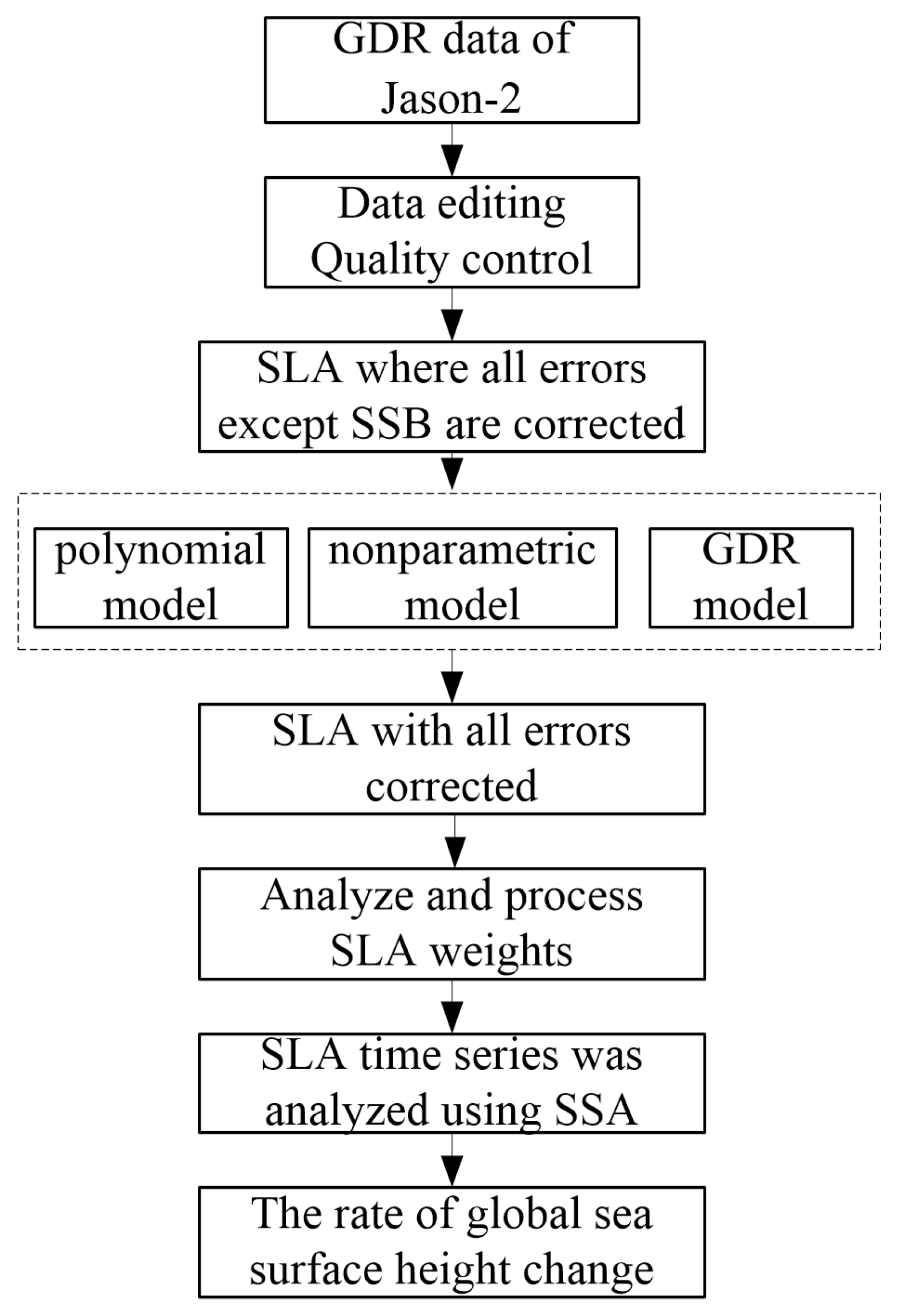
The Jason-2 GDR data and the ERA5 reanalysis data were used to study the SSB corrections based on crossover data. A parametric SSB model and a non-parametric SSB model for correcting the Jason-2 altimeter data were built in this study. The precision analysis and application of the two models were also determined in this study. The non-parametric regression estimation model, based on SWH and wind speed, improved the SSH accuracy of the Jason-2 altimeter’s data.

Based on the 1-Hz, Ku-band GDR data from cycle201 to cycle300 of the Jason-2 altimeter and the wind speed of ERA5, the LLR estimator, the Epanechnikov kernel function and the local window width were selected to construct the non-parametric regression estimation method.

Based on the Taylor expansion, 32 types of polynomial SSB models were constructed by using the 1-Hz GDR data from cycle201–cycle300 in the Ku band of the Jason-2 altimeter, with the SWH and wind speed as variables. These polynomial models were tested for the determination coefficient. The larger the determination coefficient, the higher the goodness of fit of the model. Among the 32 models, the polynomial model with six parameters had the largest determination coefficient, which indicated that the polynomial model with six parameters had the highest goodness of fit. Therefore, the optimal model was the polynomial model with six parameters.

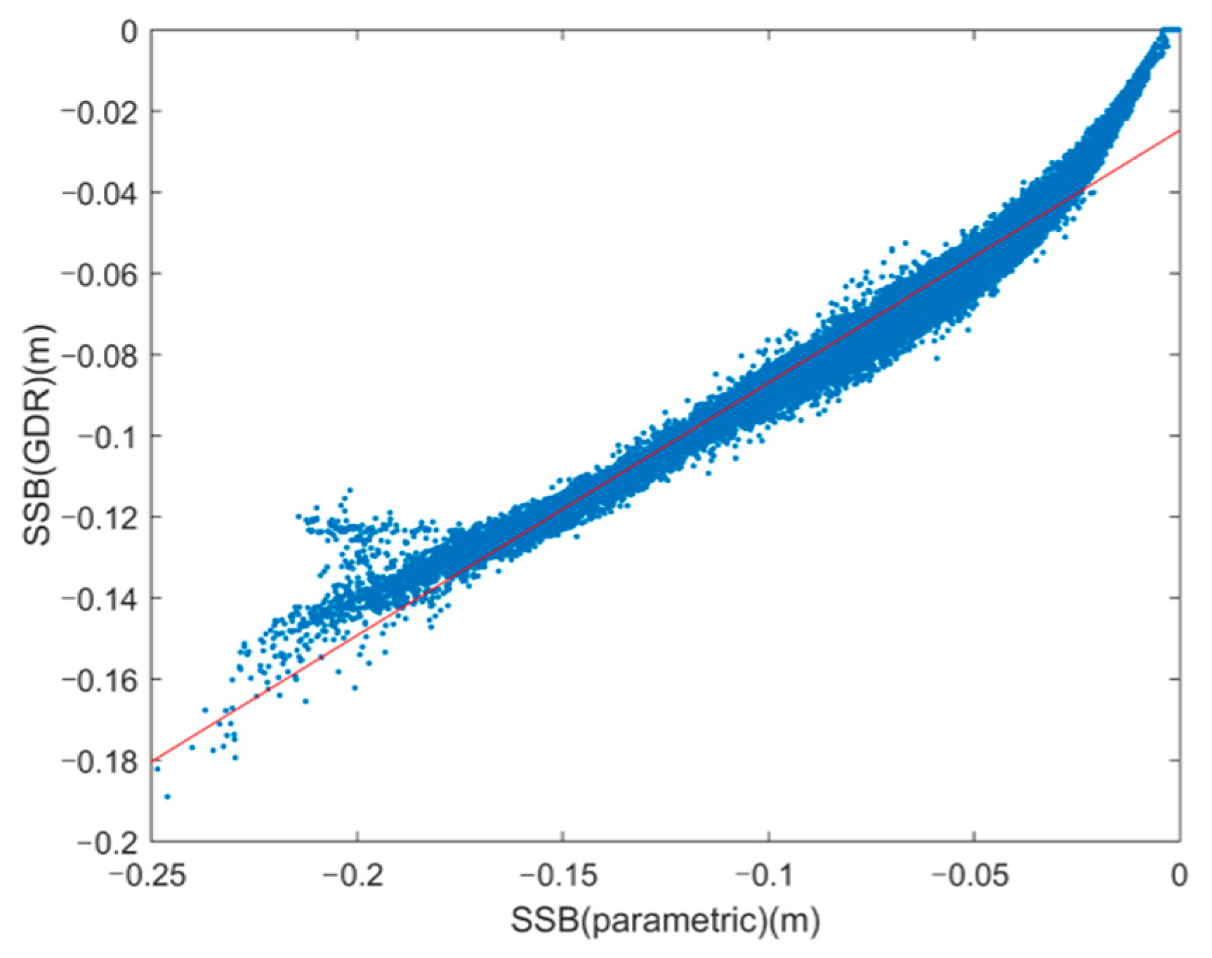
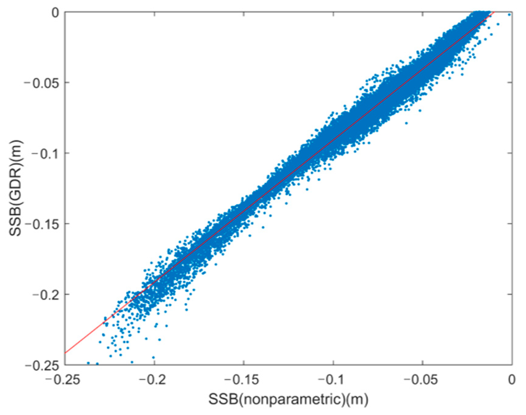
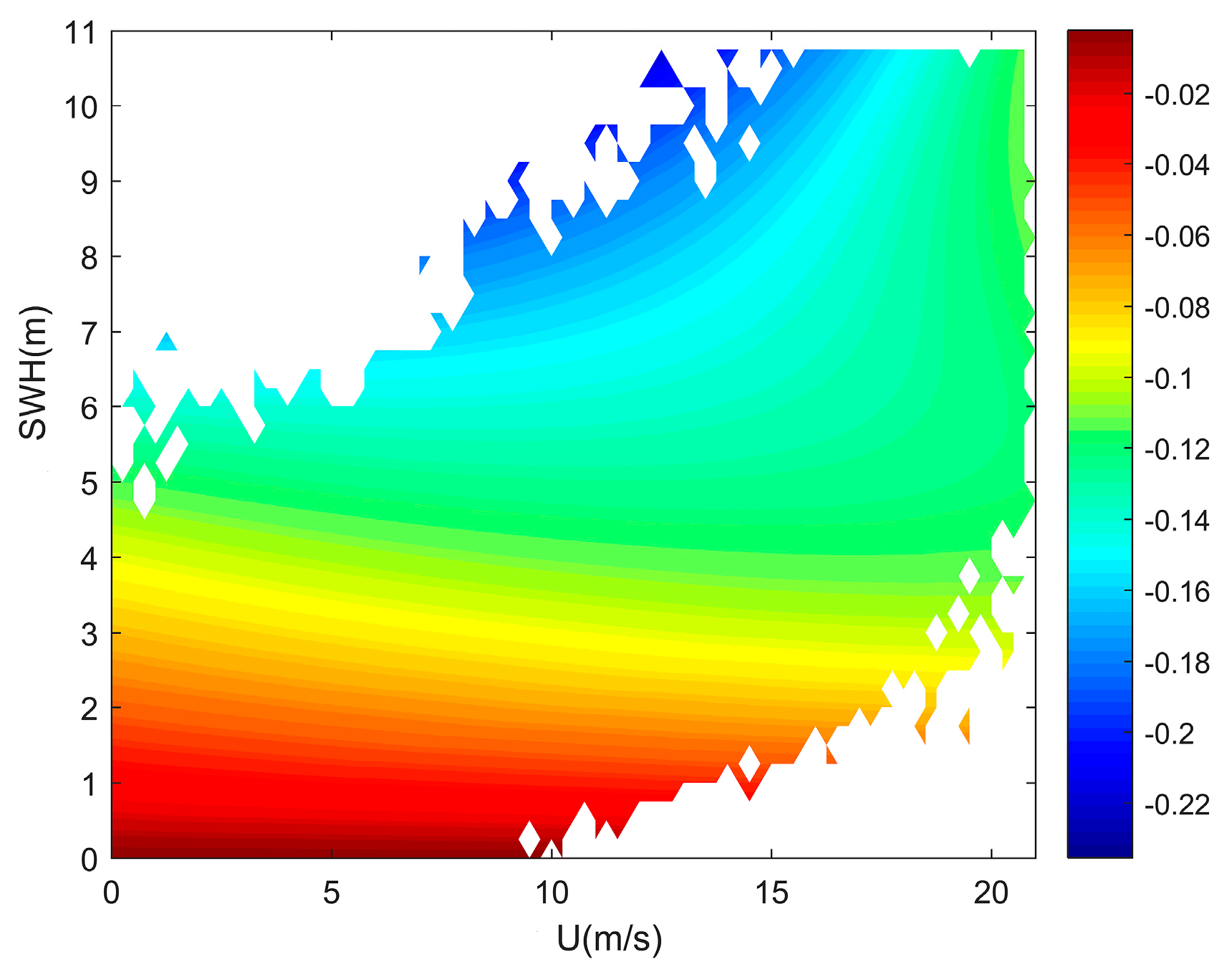
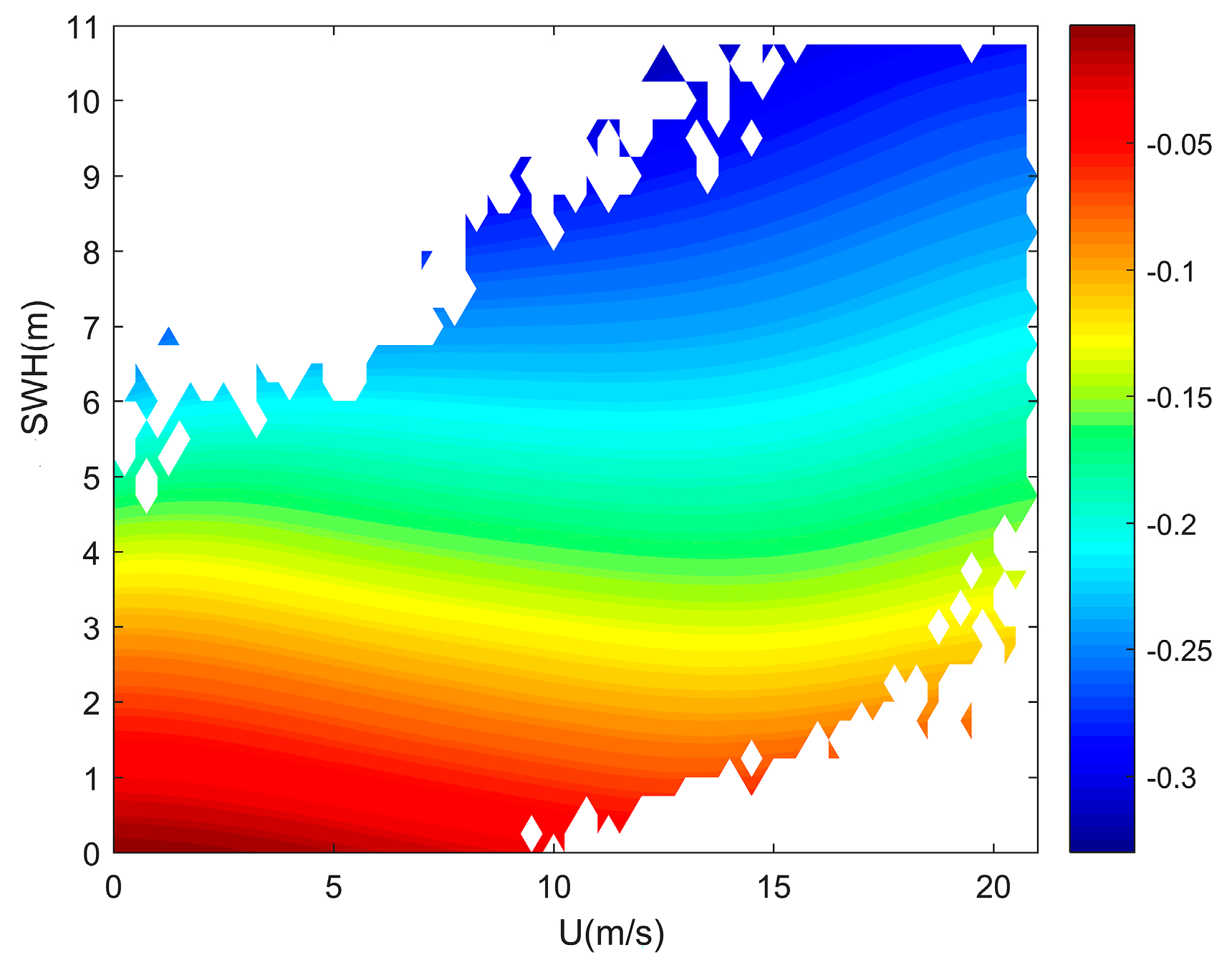
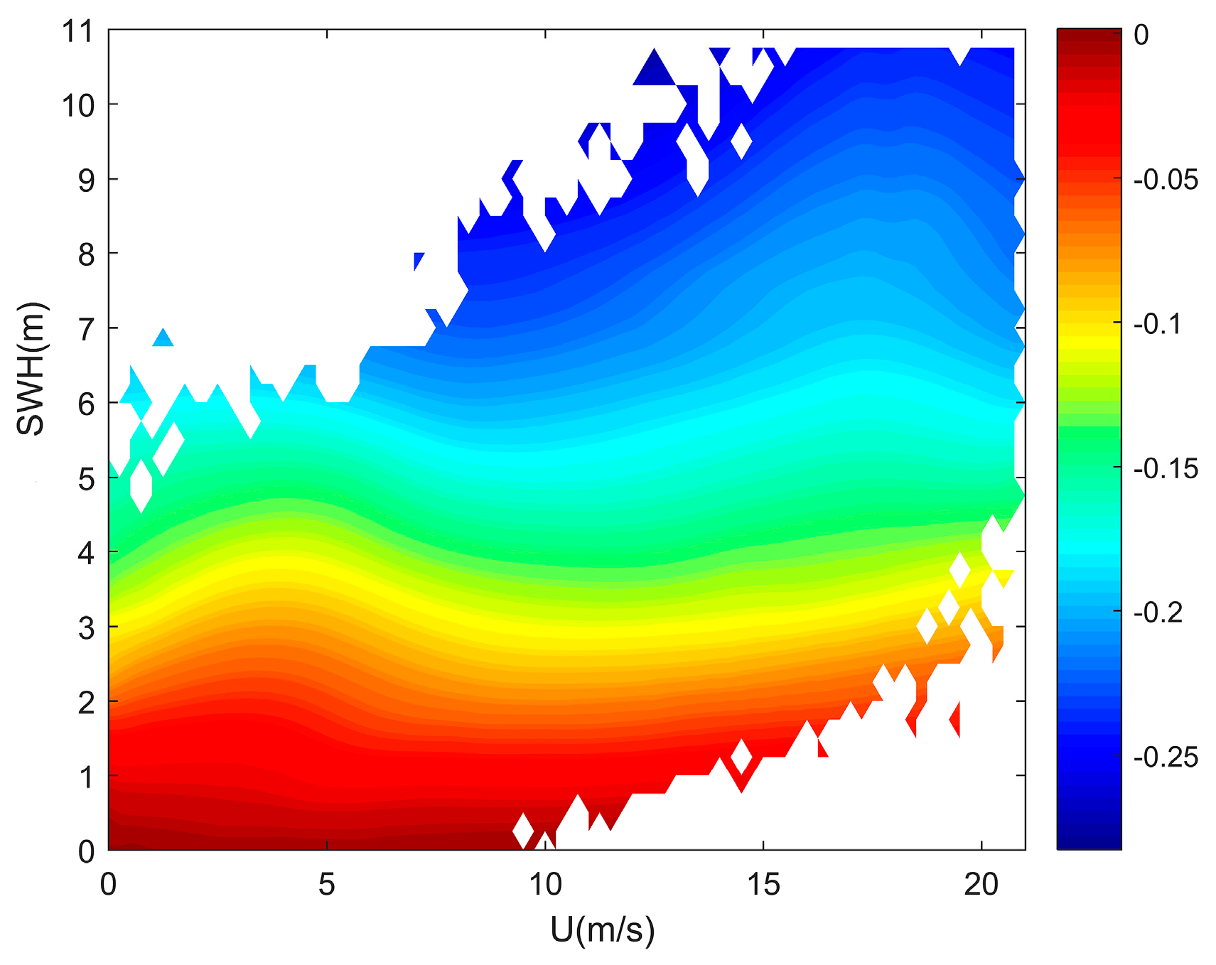
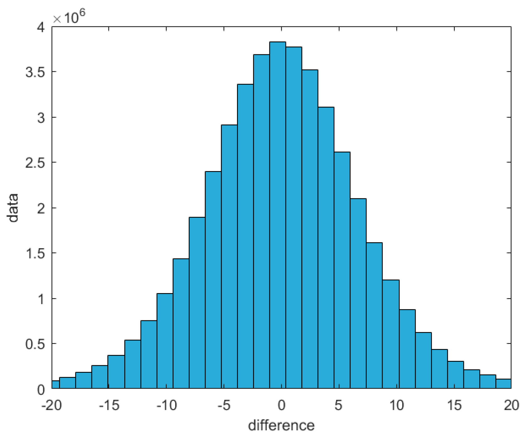
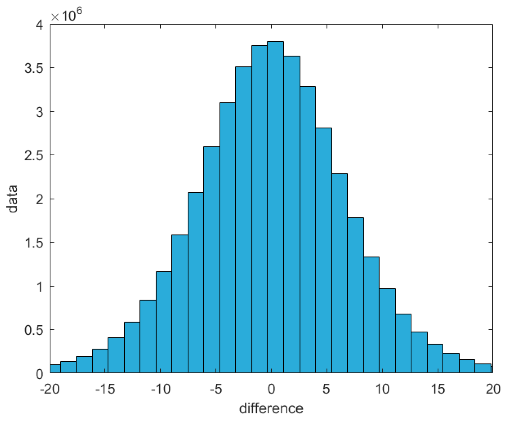
By comparing the SSBs obtained from the polynomial model and the non-parametric regression estimation model, using the GDR SSB, we saw that the RMSs of the differences between them were 2.0 cm and 1.1 cm, respectively. Therefore, the overall data fitting effect was good, and the results of the non-parametric regression estimation model and the GDR model were closer.

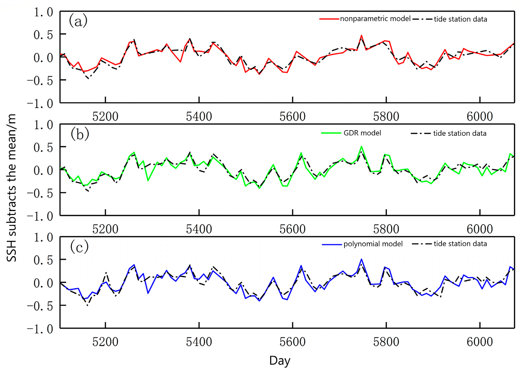
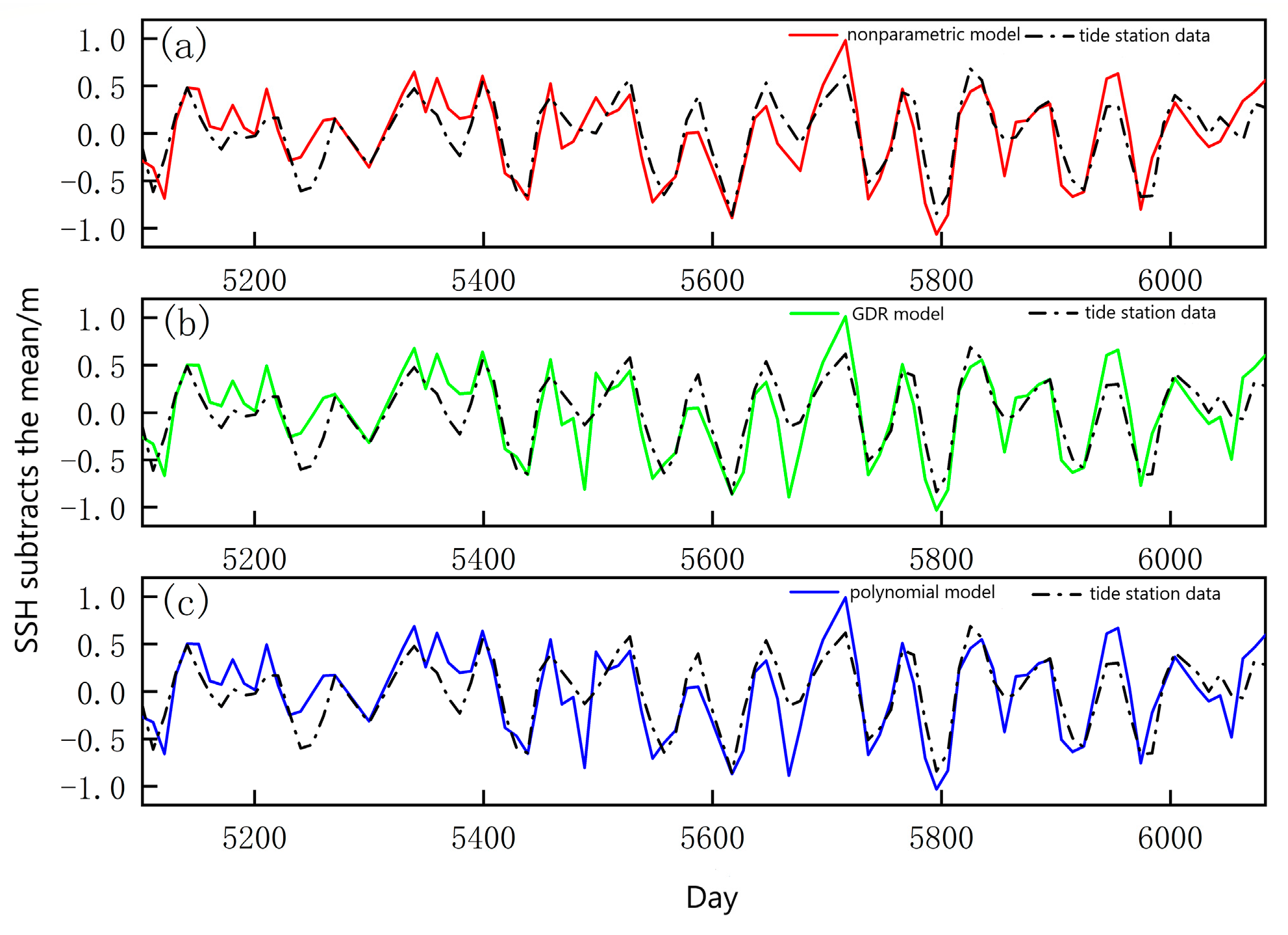
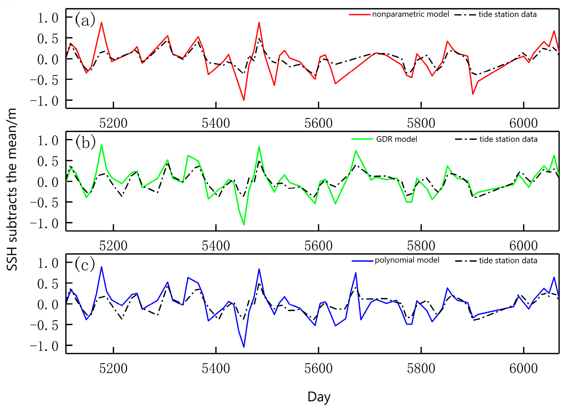
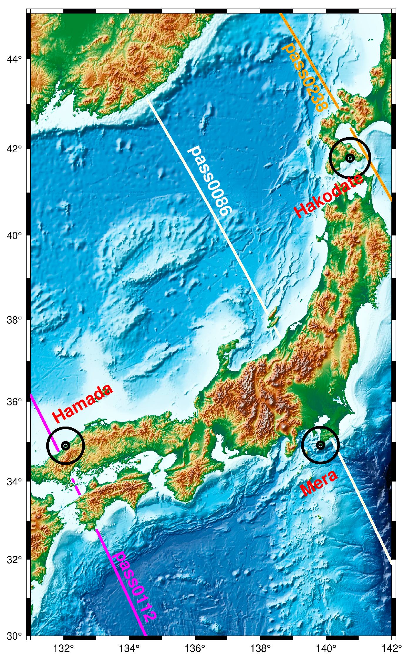
According to our analysis of the crossover SSHs and the tide gauge records—compared with the polynomial model and the GDR model—the RMS of the crossover discrepancies of SSH, which was calculated by the non-parametric regression estimation model, decreased by 7.9% and 4.1%, respectively. The STD of the differences between the corrected SSHs and the tide data decreased by 4.3–11.1% and 1.8–10.5%, respectively.

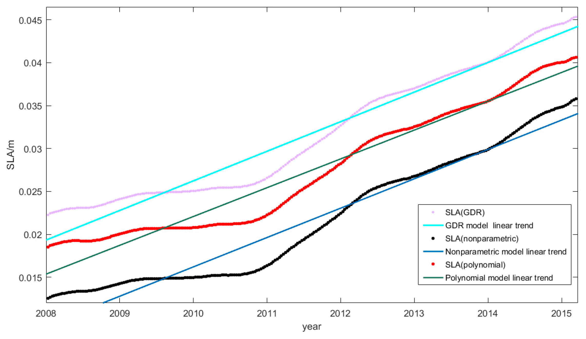
Based on the global along-track geoid gradient and the global sea-level change rate calculated by the two models constructed in this paper and compared with the calculation of the polynomial model and the GDR model, the RMS of the along-track geoid gradient difference calculated by the non-parametric regression estimation model and the vertical deviation model decreased by 2.8% and 2.4%, respectively. The along-track geoid gradient accuracy obtained by the non-parametric regression estimation model was the best. When it used SSA to analyze the 7-year time series of global sea level changes, the global sea-level change rate that was calculated by the three models was close to the average sea-level change rate published in the international literature.

References

1. Jin, T. Research on Global Mean Sea Level and Its Change from Multi-Oceanic Observations. Ph.D. Thesis, Wuhan University, Wuhan, China, 2010. [Google Scholar]
2. Yuan, J.; Guo, J.; Zhu, C.; Hwang, C.; Yu, D.; Sun, M.; Mu, D. High-resolution sea level change around China seas revealed through multi-satellite altimeter data. Int. J. Appl. Earth Obs. Geoinf. 2021, 102, 102433. [Google Scholar] [CrossRef]
3. Zhao, C.; Ou, J.; Sheng, C.; Zhang, X. Jason-2 orbit determination based on DORIS data. Prog. Geophys. 2013, 28, 49–57. [Google Scholar] [CrossRef]
4. Labroue, S.; Gaspar, P.; Dorandeu, J.; Zanife, O.; Mertz, F.; Vincent, P.; Choquet, D. Nonparametric estimates of the sea state bias for the Jason-1 radar altimeter. Mar. Geod. 2004, 27, 453–481. [Google Scholar] [CrossRef]
5. Jackson, F.C. The reflection of impulses from a nonlinear random sea. J. Geophys. Res. Oceans 1979, 84, 4939–4943. [Google Scholar] [CrossRef]
6. Longuet-Higgins, M.S. The effect of non-linearities on statistical distributions in the theory of sea waves. J. Fluid Mech. 1963, 17, 459–480. [Google Scholar] [CrossRef]
7. Srokosz, M.A. On the joint distribution of surface elevation and slopes for a nonlinear random sea with an application to radar altimetry. J. Geophys. Res. Oceans 1986, 91, 995–1006. [Google Scholar] [CrossRef]
8. Fu, L.L.; Glazman, R. The effect of the degree of wave development on the sea state bias in radar altimetry measurement. J. Geophys. Res. Oceans 1991, 96, 829–834. [Google Scholar] [CrossRef]
9. Elfouhaily, T.; Thompson, D.R.; Chapron, B.; Vandemark, D. Improved electromagnetic bias theory: Inclusion of hydrodynamic modulations. J. Geophys. Res. Oceans 2001, 106, 4655–4664. [Google Scholar] [CrossRef]
10. Arnold, D.V. Electromagnetic Bias in Radar Altimetry at Microwave Frequencies. Ph.D. Thesis, Massachusetts Institute of Technology, Cambridge, MA, USA, 1992. [Google Scholar]
11. Millet, F.W.; Warnick, K.F.; Nagel, J.R.; Arnold, D.V. Physical optics-based electromagnetic bias theory with surface height-slope cross-correlation and hydrodynamic modulation. IEEE Trans. Geosci. Remote Sens. 2006, 44, 1470–1483. [Google Scholar] [CrossRef]
12. Gaspar, P.; Ogor, F.; Le Traon, P.Y.; Zanife, O.Z. Estimating the sea state bias of the TOPEX and POSEIDON altimeters from crossover differences. J. Geophys. Res. Oceans 1994, 99, 24981–24994. [Google Scholar] [CrossRef]
13. Chelton, D.B. The sea state bias in altimeter estimates of sea level from collinear analysis of TOPEX data. J. Geophys. Res. Oceans 1994, 99, 24995–25008. [Google Scholar] [CrossRef]
14. Passaro, M.; Nadzir, Z.; Quartly, G. Improving the precision of sea level data from satellite altimetry with high-frequency and regional sea state bias corrections. Remote Sens. Environ. 2018, 218, 245–254. [Google Scholar] [CrossRef]
15. Peng, F.; Deng, X. Improving precision of high-rate altimeter sea level anomalies by removing the sea state bias and in-tra-1-Hz covariant error. Remote Sens. Environ. 2020, 218, 245–454. [Google Scholar] [CrossRef]
16. Gaspar, P.; Florens, J.P. Estimation of the sea state bias in radar altimeter measurements of sea level: Results from a new nonparametric method. J. Geophys. Res. Oceans 1998, 103, 15803–15814. [Google Scholar] [CrossRef]
17. Gaspar, P.; Labroue, S.; Ogor, F.; Lafitte, G.; Marchal, L.; Rafanel, M. Improving nonparametric estimates of the sea state bias in radar altimeter measurements of sea level. J. Atmos. Ocean. Technol. 2002, 19, 1690–1707. [Google Scholar] [CrossRef]
18. Vandemark, D.; Tran, N.; Beckley, B.D.; Gaspar, P. Direct estimation of sea state impacts on radar altimeter sea level measurements. Geophys. Res. Lett. 2002, 29, 2148–2151. [Google Scholar] [CrossRef]
19. Tran, N.; Labroue, S.; Philipps, S.; Bronner, E.; Picot, N. Overview and update of the sea state bias corrections for the Jason-2, Jason-1 and TOPEX missions. Mar. Geod. 2010, 33 (Suppl. S1), 348–362. [Google Scholar] [CrossRef]
20. Tran, N.; Thibaut, P.; Poisson, J.C.; Philipps, S. Impact of Jason-2 wind speed calibration on the sea state bias correction. Mar. Geod. 2010, 34, 407–419. [Google Scholar] [CrossRef]
21. Benassai, G.; Migliaccio, M.; Montuori, A.; Ricchi, A. Wave simulations through Sar Cosmo-Skymed wind retrieval and verification with buoy data. In Proceedings of the Twenty-Second (2012) International Offshore and Polar Engineering Conference, Rhodes, Greece, 17–22 June 2012. [Google Scholar]
22. Jiang, M. Study on the Errors Correction and Ocean-Land Echo Waveforms Processing for HY-2A Radar Altimeter. Ph.D. Thesis, National Space Science Center, Chinese Academy of Sciences, Beijing, China, 2018. [Google Scholar]
23. Zhong, G.; Liu, B.; Guo, Y.; Miao, H. Sea state bias estimation with least absolute shrinkage and selection operator (LASSO). J. Ocean Univ. China 2018, 17, 1019–1025. [Google Scholar] [CrossRef]
24. Zhong, G.; Qu, J.; Wang, H.; Liu, B.; Jiao, W.; Fan, Z.; Miao, H.; Hedjam, R. Trace-Norm regularized multi-task learning for sea state bias estimation. J. Ocean Univ. China 2020, 19, 1292–1298. [Google Scholar] [CrossRef]
25. Shao, W.; Hu, Y.; Zheng, G.; Cai, L.; Yuan, X.; Zou, J. Sea state parameters retrieval from cross-polarization Gaofen-3 SAR data. Adv. Space Res. 2020, 65, 1025–1034. [Google Scholar] [CrossRef]
26. Quilfen, Y.; Chapron, B. On denoising satellite altimeter measurements for high-resolution geophysical signal analysis. Adv. Space Res. 2020, 68, 875–891. [Google Scholar] [CrossRef]
27. Taqi, A.; Al-Subhi, A.; Alsaafani, M.; Abdulla, C. Improving sea level anomaly precision from satellite altimetry using parameter correction in the red sea. Remote Sens. 2020, 12, 764. [Google Scholar] [CrossRef]
28. Chu, C.K.; Marron, J.S. Choosing a kernel regression estimator (with discussions). Stat. Sci. 1991, 6, 404–419. [Google Scholar] [CrossRef]
29. Fan, J.; Gijbels, I. Local Polynomial Modelling and Its Applications; Chapman and Hall: New York, NY, USA, 1996. [Google Scholar]
30. Fan, J. Design-adaptative nonparametric regression. J. Am. Stat. Assco. 1992, 87, 998–1004. [Google Scholar] [CrossRef]
31. Wand, M.P.; Jones, M.C. Kernel Smoothing; Chapman and Hall: New York, NY, USA, 1995. [Google Scholar]
32. Simonoff, J.S. Smoothing categorical data. J. Stat. Plan. Infer. 1995, 47, 41–69. [Google Scholar] [CrossRef]
33. Hall, P. On the bias of variable bandwidth curve estimators. Biometrika 1990, 77, 529–535. [Google Scholar] [CrossRef]
34. Abramson, I.S. On bandwidth variation in kernel estimates-a square root law. Ann. Stat. 1982, 10, 1217–1223. [Google Scholar] [CrossRef]
35. Guo, J.; Hou, R.; Zhou, M.; Jin, X.; Li, G. Detection of particulate matter changes caused by 2020 california wildfires based on gnss and radiosonde station. Remote Sens. 2021, 13, 4557. [Google Scholar] [CrossRef]
36. Dumont, J.; Rosmorduc, V.; Picot, N.; Desai, S.; Bonekamp, H.; Figa, J.; Lillibridge, J.; Scharroo, R. OSTM/Jason-2 Products Handbook. CNES: SALP-MU-M-OP-15815-CN, EUMETSAT: EUM/OPS-JAS/MAN/08/0041, JPL: OSTM-29-1237, NOAA/NESDIS: Polar Series/OSTM OSTM J, 400. 2011. Available online: https://www.aviso.altimetry.fr/fileadmin/documents/data/tools/hdbk_j2.pdf (accessed on 2 December 2021).
37. Hersbach, H.; Bell, B.; Berrisford, P.; Hirahara, S.; Horányi, A.; Muñoz-Sabater, J.; Nicolas, J.; Peubey, C.; Radu, R.; Schepers, D.; et al. The ERA5 global reanalysis. Q. J. R. Meteorol. Soc. 2020, 146, 1999–2049. [Google Scholar] [CrossRef]
38. Dee, D.; Uppala, S.; Simmons, A.; Berrisford, P.; Poli, P.; Kobayashi, S.; Andrae, U.; Balmaseda, M.; Balsamo, G.; Bauer, P.; et al. The ERA-Interim reanalysis: Configuration and performance of the data assimilation system. Q. J. R. Meteorol. Soc. 2011, 137, 553–597. [Google Scholar] [CrossRef]
39. Caldwell, P.C.; Merrifield, M.A.; Thompson, P.R. Sea level measured by tide gauges from global oceans—The Joint Archive for Sea Level holdings (NCEI Accession 0019568), Version 5.5, NOAA National Centers for Environmental Information. Dataset 2015, 10, V5V40S7W. [Google Scholar]
40. Sandwell, D.T.; Harper, H.; Tozer, B.; Smith, W.H.F. Gravity field recovery from geodetic altimeter missions. Adv. Space Res. 2021, 68, 1059–1072. [Google Scholar] [CrossRef]
41. Yuan, J. Mean Sea Surface Modeling and Fine Sea Level Change from Multi-Satellite Altimetry Data. Ph.D. Thesis, Shandong University of Science And Technology, Shandong, China, 2021. [Google Scholar]
42. Hou, K.; Zhang, S.; Kong, X. Quality assessment of HY-2A altimeter data through tide gauge comparisons. Haiyang Xuebao 2019, 41, 136–142. [Google Scholar] [CrossRef]
43. Li, Z.; Guo, J.; Ji, B.; Wan, X.; Zhang, S. A review of marine gravity field recovery from satellite altimetry. Remote Sens. 2022, 14, 4790. [Google Scholar] [CrossRef]
44. Zhu, C.; Guo, J.; Yuan, J.; Li, Z.; Liu, X.; Gao, J. SDUST2021GRA: Global marine gravity anomaly model recovered from Ka-band and Ku-band satellite altimeter data. Earth Syst. Sci. Data 2022, 14, 4589–4606. [Google Scholar] [CrossRef]
45. Zhou, M.; Guo, J.; Shen, Y.; Kong, Q.; Yuan, J. Extraction of common mode errors of GNSS coordinate time series based on multi-channel singular spectrum analysis. Chin. J. Geophys. 2018, 61, 67–79. [Google Scholar] [CrossRef]
46. IPCC. Climate Change 2021 the Physical Science Basis; Cambridge University Press: Cambridge, UK, 2021.
47. Nerem, R.S.; Beckley, B.D.; Fasullo, J.T.; Hamlington, B.D.; Masters, D.; Mitchum, G.T. Climate-change-driven accelerated sea-level rise detected in the altimeter era. Proc. Natl. Acad. Sci. USA 2018, 115, 2022–2025. [Google Scholar] [CrossRef]
48. Cazenave, A.; Dieng, H.B.; Meyssignac, B.; Schuckmann, K.; Decharme, B.; Berthier, E. The rate of sea-level rise. Nat. Clim. Chang. 2014, 4, 358–361. [Google Scholar] [CrossRef]
Figure 1. Scatterplot of the polynomial model with SSB of GDR.
Remotesensing 15 02666 g001
Figure 2. Scatterplot of non-parametric regression estimation model with SSB of GDR.
Remotesensing 15 02666 g002
Figure 3. (a) Time series of altimetry data from the non-parametric model and Hamada tide gauge records; (b) time series of altimetry data from the GDR model and Hamada tide gauge records; and (c) time series of altimetry data from the polynomial model and Hamada tide gauge records.
Remotesensing 15 02666 g003
Figure 4. (a) Time series of altimetry data from the non-parametric model and Mera tide gauge records; (b) time series of altimetry data from the GDR model and Mera tide gauge records; and (c) time series of altimetry data from the polynomial model and Mera tide gauge records.
Remotesensing 15 02666 g004
Figure 5. (a) Time series of altimetry data from the non-parametric model and Hakodate tide gauge records; (b) time series of altimetry data from the GDR model and the Hakodate tide gauge records; and (c) time series of altimetry data from the polynomial model and the Hakodate tide gauge records.
Remotesensing 15 02666 g005
Figure 6. SSBs of the polynomial model (m).
Remotesensing 15 02666 g006
Figure 7. SSBs of the non-parametric regression estimation model plane (m).
Remotesensing 15 02666 g007
Figure 8. SSBs in GDR (m).
Remotesensing 15 02666 g008
Figure 9. Histogram of the differences between along-track geoid gradients, calculated by the polynomial model and the SIO V30.1_DOV model (the x-coordinate is in μrad).
Remotesensing 15 02666 g009
Figure 10. Histogram of the differences between along-track geoid gradients calculated by the GDR model and the SIO V30.1_DOV model (the x-coordinate is in μrad).
Remotesensing 15 02666 g010
Figure 11. Histogram of the differences between along-track geoid gradients calculated by the non-parametric regression estimation model and the SIO V30.1_DOV model (the x-coordinate is in μrad).
Remotesensing 15 02666 g011
Figure 12. Global sea level change.
Remotesensing 15 02666 g012