1. Introduction
Synthetic Aperture Radar (SAR) [
1] uses echo coherence processing to obtain high-resolution images. SAR images have been widely used in the fields of military target detection and civilian remote sensing. The research of automatic target recognition technology [
2,
3] based on two-dimensional SAR images with high resolution has important military and civilian values. With the development of Convolution Neural Networks (CNN), the recognition of SAR images using CNN [
4,
5] has been studied intensively. Gao et al. [
6] propose a multi-feature fusion network and the weighted distance classifier to extract classification features and classify them. The neural network performs excellently in learning offline data. However, the neural network is less effective with streaming data for SAR images. When updating the model with new data, the data representation and decision boundary are changed. The model will rapidly forget what it has learned previously with the change of parameters, this is called catastrophic forgetting [
7]. The most primitive method to deal with the forgetting problem is to use all data to retrain the whole model whenever a new task comes. However, retraining will waste a lot of time, and the model will collapse when the data increases to unaffordable status. Furthermore, in some realistic situations, the samples from previous classes are often difficult to obtain at once. It is impossible for the model to retain all data.
Class-Incremental Learning (CIL) [
8], also called Continue Learning (CL) [
9], Life-Long Learning (LLL) [
10], solves the problem of learning from streaming data and gives the possibility for the model to learn new tasks continually. The major challenge of CIL is that performance on previous tasks cannot significantly decrease with new tasks added. The aim is to find a better trade-off between the plasticity and stability of the model [
11], where plasticity refers to the ability to integrate new information from new tasks and stability is to retain previous knowledge while learning it. Instead of retraining the entire model, CIL introduces various methods to make the model learn continually, such as the replay strategy [
12,
13,
14], regularization-based methods [
15,
16] and parameter isolation method [
17]. Previous works widely adopt the replay strategy: storing small samples of old classes and reusing them when the model learns new classes. For example, Rebuffi et al. [
12] proposed a Herding-based preferential samples selection method (iCaRL). Wu et al. [
18] optimized the classification bias in the extracted samples (BiC). However, this kind of method only reshows a few samples from old classes. Since the number of retained samples is less than those from new classes, the distribution of features in the old and new classes is unbalanced. The model prefers to learn new classes. As a result, it is still challenging to alleviate forgetting only under the replay strategy. Convinced by this fact, we highlight two major barriers to be addressed for CIL: (i) Besides repaying samples of old classes, how can we keep the knowledge alive in the future? (ii) Under the limited structure and storage space, how can we store more information to recreate a similar situation in the past?
Complementary Learning Systems (CLS) theory [
19] researches the memory style of mammals. When recalling past scenes, mammals will construct a new insight under the guidance of the current scenario. For example, people’s attitudes toward others change with experience. This memory pattern is gradually being used in incremental learning to reduce the forgetting of models. In Natural Language Processing (NLP), prompt-based learning (prompting) [
20] is a new transfer learning technique developed from CLS theory. Prompting techniques design inputs with templated or learnable prompt tokens. These prompt tokens contain additional task information, allowing the language model to obtain more information from the input. Incremental methods from CLS theory and prompting techniques handle the CIL problems to a certain extent. For instance, in incremental learning, Wang, et al. [
21] propose a trainable prompt pool module to store encoded knowledge (L2P). However, L2P is a method of freezing the feature extraction layer and only training the classifier [
22,
23,
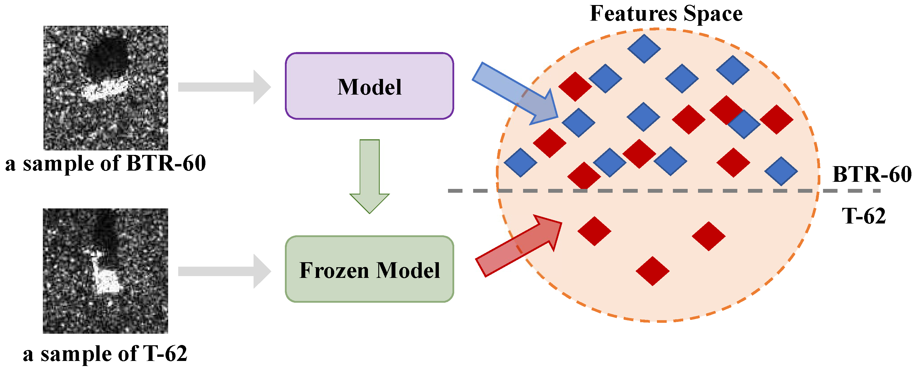
24]. When tasks are significantly different, the frozen feature extraction layer will extract similar features.
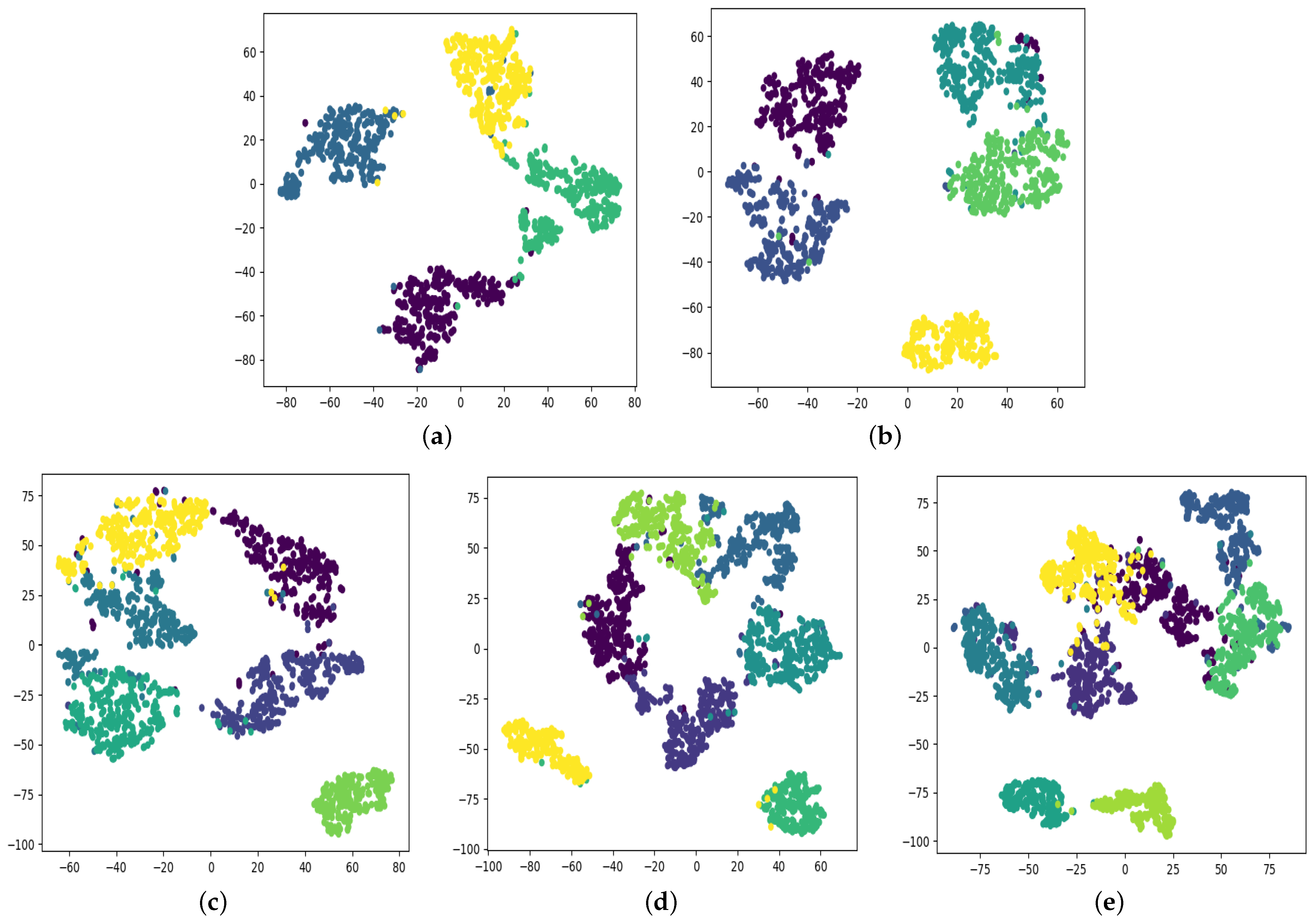
Figure 1 shows that these similar features do not represent the characteristics of tasks in the feature space and negatively affect the result of recognition. These methods are just used for akin tasks.
Motivated by the above discussions, we propose a Class-Incremental Learning method for SAR images based on self-sustainment guidance representation to maintain plasticity and stability simultaneously. In relation to plasticity, we use little storage space to store the remarkable features of different classes, and this information guides the direction of feature extraction when the model is learning. For example, it is known that some features are essential for classification, such as a pig’s nose. When samples of the pig are given, the model focuses on the nose for classification under the guidance of the special features stored before. For stability, we use extra structure to construct a bridge between the past and the future to imitate how mammals remember. The new samples go through the extra structure which is trained by previous knowledge, and its output may be the features of new classes under the old situation. The features combine with current knowledge of new classes from basic structure to assist the model’s learning.
Specifically, we built a base framework with a vision transformer (ViT) [
25] for feature extraction and classification recognition. We designed a dynamic query navigation module to maintain plasticity. The module retains the special information of classes and adds this information to the input. The direction of the feature extraction layer is changed dynamically to the current class with the guidance of special information. In addition, we also propose a structural extension module to hold the stability. The extra structure is designed to keep the model’s knowledge representation of old classes. Through the fusion of information and structural expansion of some encoding layers in the transformer encoder, the model learns under the guidance of both new and old knowledge. We introduce knowledge distillation to transfer the structural information from the extra model to the new model.
In summary, the contributions of this letter are as follows:
- (1)
We propose a learnable dynamic query navigation module to enhance the feature extraction ability of the model. The module learns and retains the special information of the class more conducive to achieving target recognition. Inputting this special information as auxiliary information can guide the focus of feature extraction of the model. The features acquired are more beneficial for classification recognition. The module can also apply to non-incremental learning models.
- (2)
We propose a structural extension module to address the catastrophic forgetting problem of the model. Considering the knowledge expressions related to the old classes, the module multi-dimensionally integrates the representation of knowledge in new and old classes. It achieves situational memory of past information rather than a simple recapitulation. The module achieves better results in preventing forgetting than the conventional replay method.
- (3)
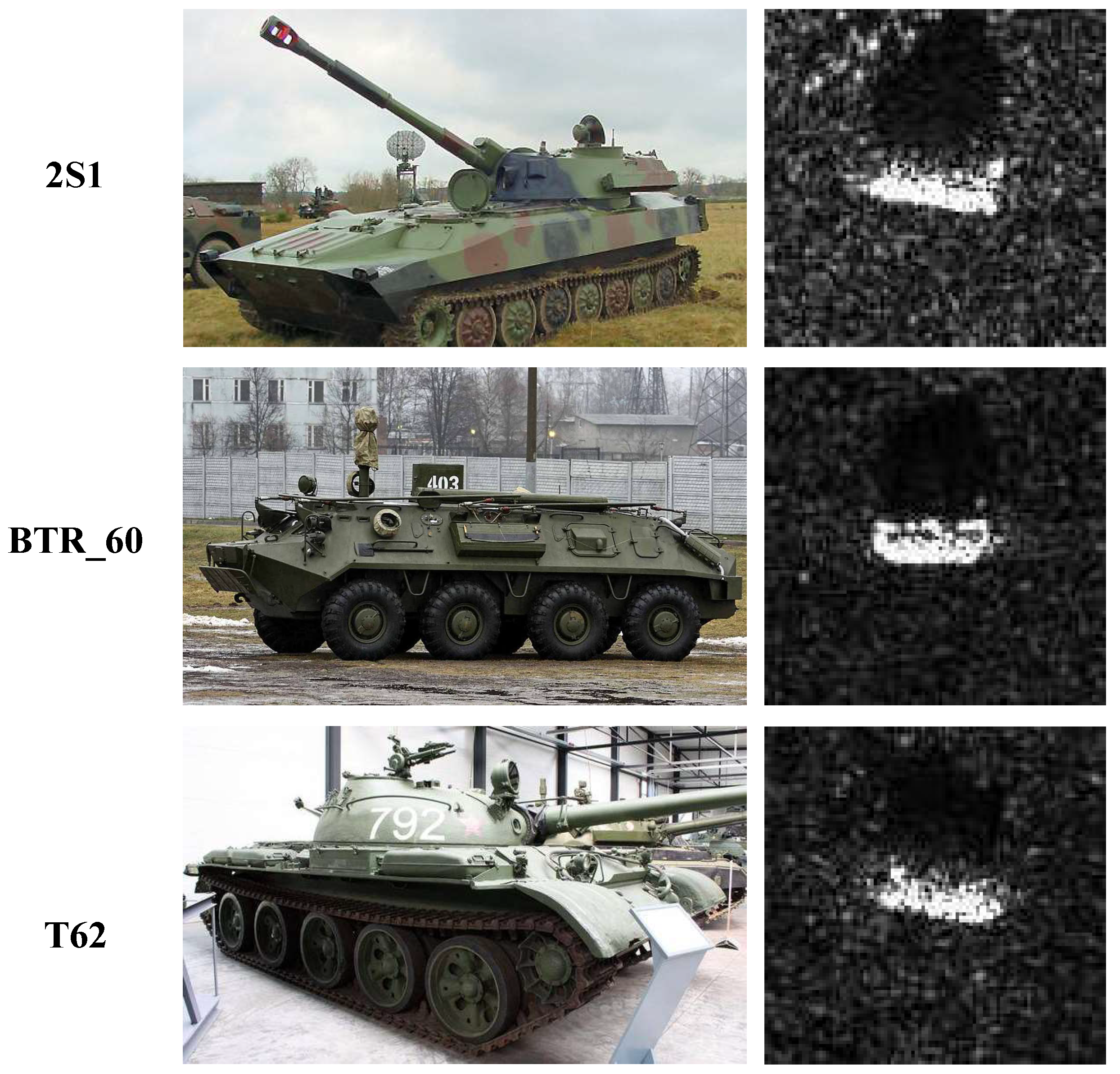
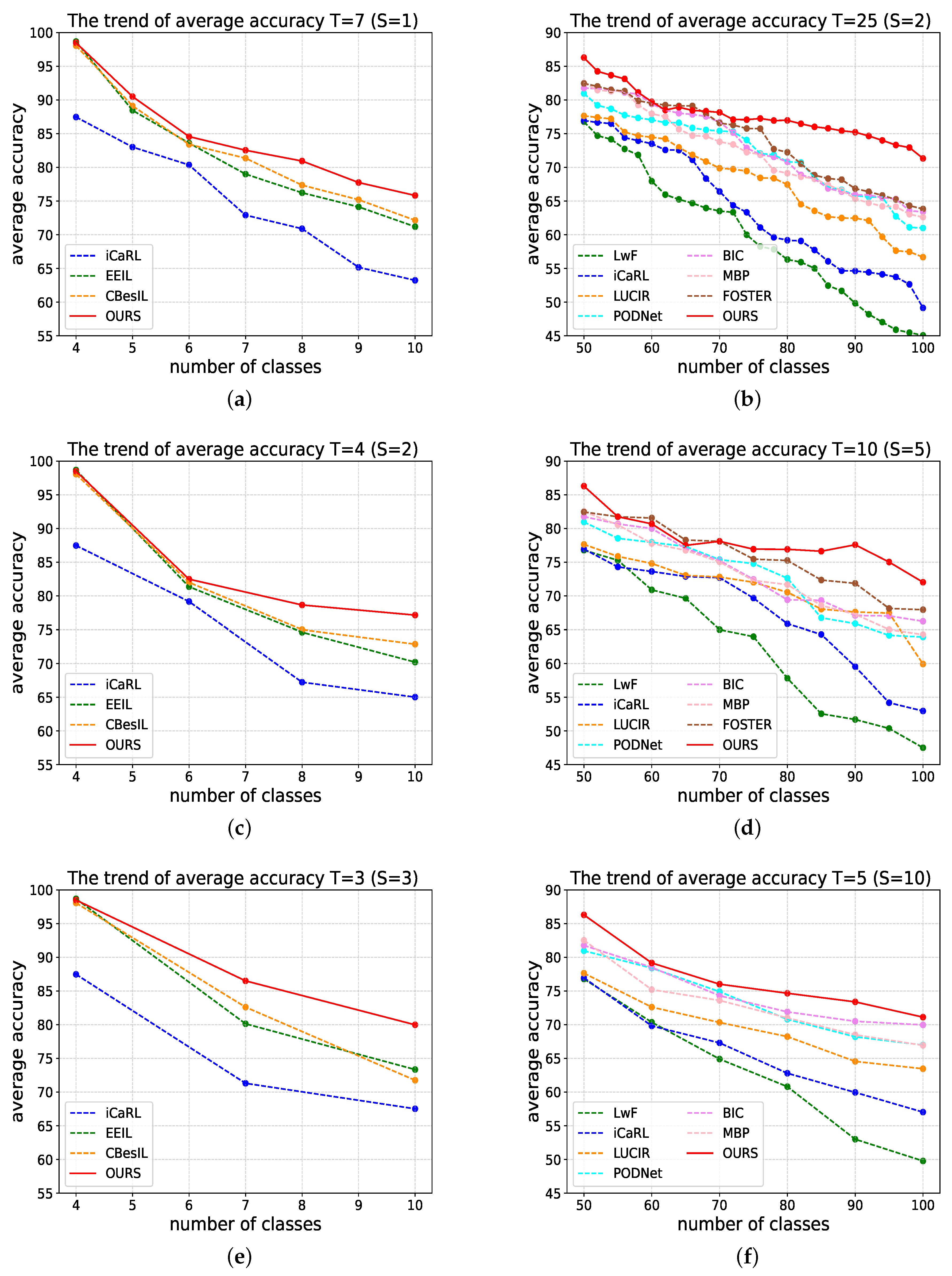
We conducted comprehensive experiments from multiple perspectives to demonstrate the effectiveness of our method. Experiments on the MSTAR SAR dataset show that our method is significantly better than existing incremental learning methods. Experiments on the CIFAR100 dataset show that our method can also be used in a more general scenario.
3. Method
In this section, we first describe the concept of Class-Incremental Learning (CIL). Afterward, we show the general structure and details of the method.
3.1. Problem Statement
Incremental learning is the process by which the model learns incrementally on a series of tasks . These tasks include data sets and label sets . In incremental learning, is called base task, are called incremental tasks. Each incremental task has the same number of new classes, and the classes do not intersect, i.e., . The goal of incremental learning is that the model learns new datasets on the current task t while maintaining the ability to recognize previous datasets .
3.2. Model Architecture
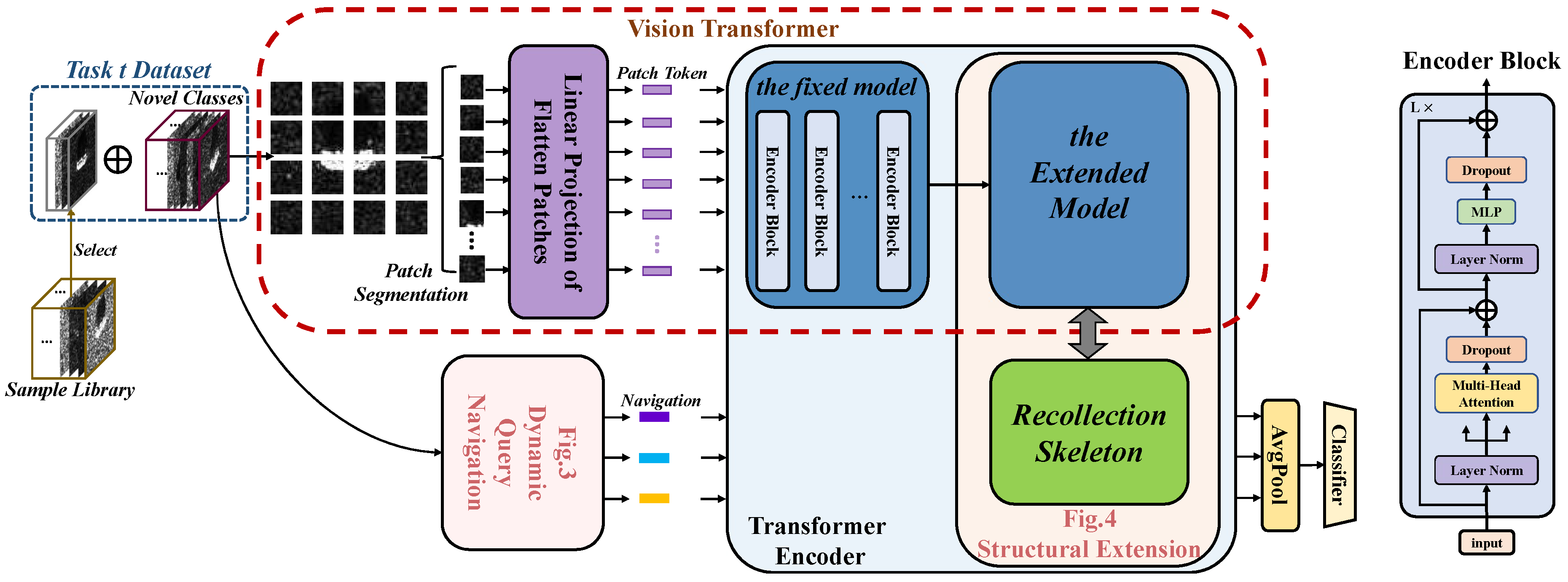
The whole structure of our model consists of three parts: a basic framework based on a vision transformer for feature extraction and classification recognition, a dynamic query navigation module for storing the special information of classes, and a structural extension module for maintaining the knowledge representation of the old classes.
Figure 2 depicts the complete structure of the model. Algorithm 1 explains the process of the overall structure of our method.
When the model is learning task
t, the training samples
of new classes are combined with selected samples
saved in the sample library:
| Algorithm 1 The Overall Structure |
Input:
image x; linear projection ; the dynamic query navigation module ;
the structural extension module |
| Hyper-parameters: Epoch number E |
Output: Prediction output - 1:
fordo - 2:
Transfer x to 1-dimensional tokens: - 3:
Transfer x to 1-dimensional navigations: - 4:
Combine the two variations: - 5:
Extract features from the fixed model: - 6:
Extract features from the structural extension module: - 7:
Calculate the average at the output of navigations: - 8:
Input classifier to obtain prediction results - 9:
- 10:
end for - 11:
return Result
|
Given an input of two-dimensional images in , where is the dimension of the images, C is the number of channels. In the first stage, the images go through two modules to obtain the input of the transformer encoder layer. On the one hand, through the linear projection layer of ViT, x is split and mapped as a series of 1-dimensional tokens , where is the number of tokens, and D is the fixed dimension of the input of VIT. On the other hand, through the dynamic query navigation module, x is transferred to a handful of one-dimensional navigations , where M is the number of navigations and D means that the navigation has the same dimension as the token. The results of the above two variations on the image x are combined as and fed into the transformer encoder for feature extraction.
In the second stage, the transformer encoder layer acting as the feature extraction layer in ViT extracts the features from . It is generally considered that the lower layers of the model can extract the basic characteristics of the target, which can be used for almost all categories with a strong generalization. Moreover, the higher layers extract the unique characteristics of the target which only be used for the single class. Therefore, as the transformer encoder consists of L encoder block layers, we divide the transformer encoder into two parts: the front layers form a fixed module for extracting general features, and the back layers form a structural extension module with the recollection skeleton.
The self-attention mechanism integrates information from all one-dimensional inputs. Every position of output contains information from other positions. Therefore, we use the output of navigations on the transformer encoder. The output is averaged and fed into a softmax classifier to obtain the recognition result of the model.
3.3. Dynamic Query Navigation Module
When people are identifying animals, they pay attention to the remarkable features of different animals, such as the red crown of the rooster, the pointed ear and striped pattern of a tabby, or the round ear and single-color pattern of the bear. However, some redundant features might negatively affect the result. For example, when identifying a rooster, both the red crown and the flattened feathers are characteristics of it. If we pay attention to all the characteristics, the incorrect answer is probably a bird with a red crown. Apparently, the marked features are what we need to pay more attention to when identifying.
The ideal model shares knowledge for similar classes while keeping knowledge independent for different classes. Like the striped pattern and the round ear can describe a tiger, these features also belong to a tabby and a bear. As a result, The shared information assists the learning of tasks similar to the past and alleviates the stress of storage.
Therefore, inspired by reference [
21], we propose the learnable navigation set
to store the remarkable information of different classes, where
N is the number of navigations. The set is shared with all tasks. We use the information to guide the direction of feature extraction by expanding the input of the transformer encoder with the navigation. For this reason, the navigation and the input of the transformer encoder should have the same dimension
D.
Furthermore, we propose a learnable key set
to choose the remarkable information which is the sample needed, where
N is the number of key vectors,
is the length of
. The key set is the bridge between the navigation and the category of the sample. On the one hand, each key and navigation are paired for finding navigations by keys. That means the number of keys and the number of navigations is the same, denoted as
. On the other hand, in order to obtain the probable category of the sample, we introduce a backbone vision transformer model to pre-classify it. The backbone model uses the basic structure from the reference [
25], and the parameters were pre-trained on the Google private dataset (JFT-300M). By computing the similarities between keys and the query features
from the backbone model, we can choose the special information the sample needs. As a result, the key and the query features should have the same dimension
.
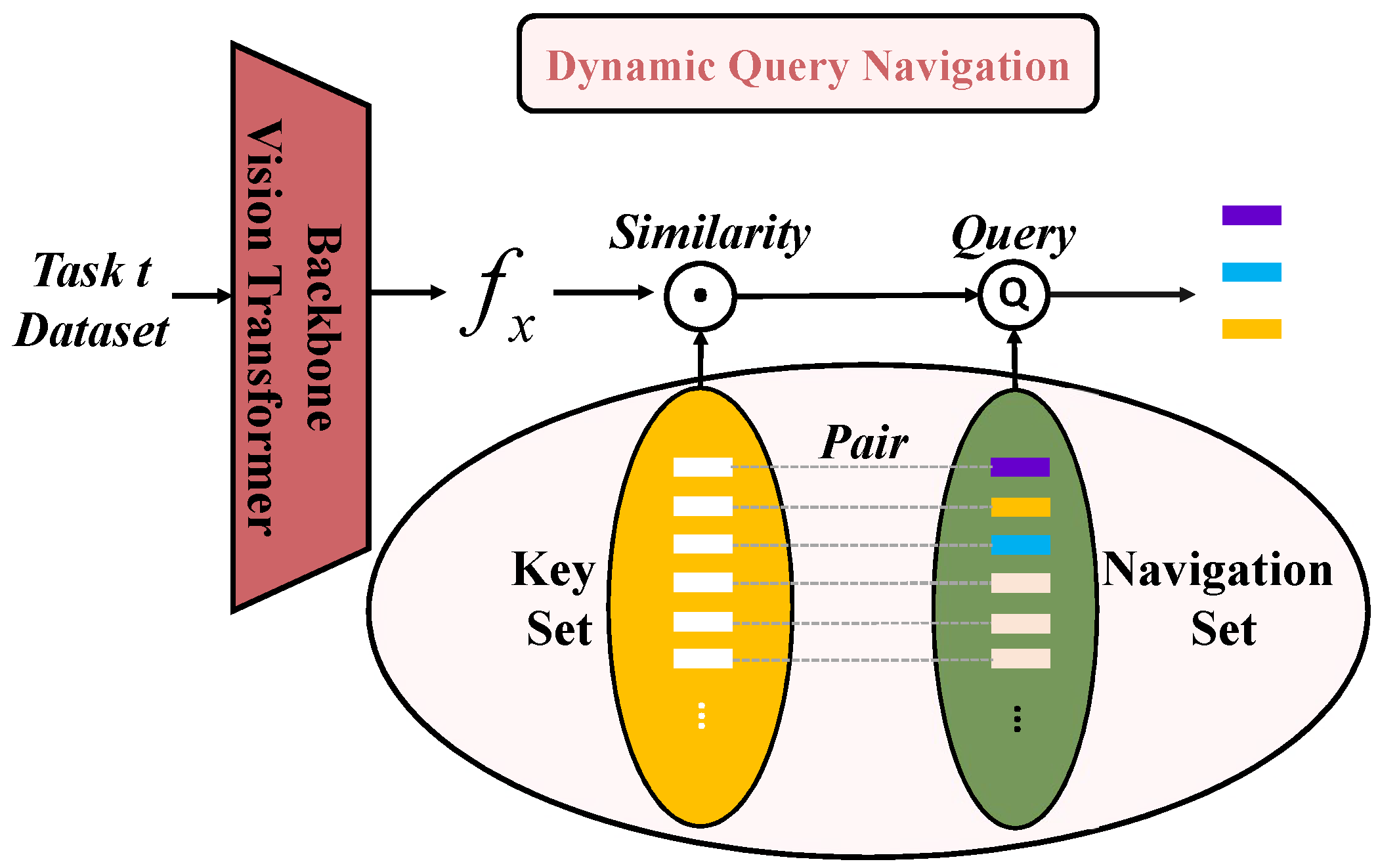
As shown in
Figure 3, the whole dynamic query navigation module consists of a navigation set, a key set and a backbone vision transformer model. Algorithm 2 explains the training and testing process of this module.
| Algorithm 2 The process of the dynamic query navigation module |
| Input: image x; backbone ViT model |
Output: Chosen navigations - 1:
Pre-classify the image by backbone ViT model: - 2:
Calculate the similarity between key and by Equation ( 2) - 3:
Choose indexes of the first M maximum similarities - 4:
Choose the correspond navigations from index - 5:
return
|
When training the model, keys and navigations are trained to obtain the information of the current samples. When testing, the current sample is put into the backbone model to obtain the query features
of their potential class. We then calculate the similarity between query features
and all keys in the key set:
where
is the
parametrization.
The indexes of the key of the first M maximum similarities are taken and according to the correspondence between keys and navigation, the first M navigations are queried. is the remarkable information of classes we wish to obtain for identification.
3.4. Structural Extension
The CLS theory in neuroscience suggests that mammals have two learning systems: the neocortex and the hippocampus. The hippocampus rapidly replays recently learned memories, integrating them as interconnections of neocortical neurons and becoming a more solid memory. Based on this, we construct an extra structure called the recollection skeleton as the neocortex to store the solid memory of the past. The feature extraction layer acts as the hippocampus for learning new knowledge. In addition, the research also shows that the hippocampus does not directly recall past events when replaying memories, but constructs a new insight called situational memory, according to a realistic scenario. For machine learning, we consider the output of the new data on the old model as the memory associated with the old class, equivalent to the situational memory of the hippocampus. Since we have constructed the recollection skeleton to store parameters of the old model, the new data is put through it to recall past knowledge.
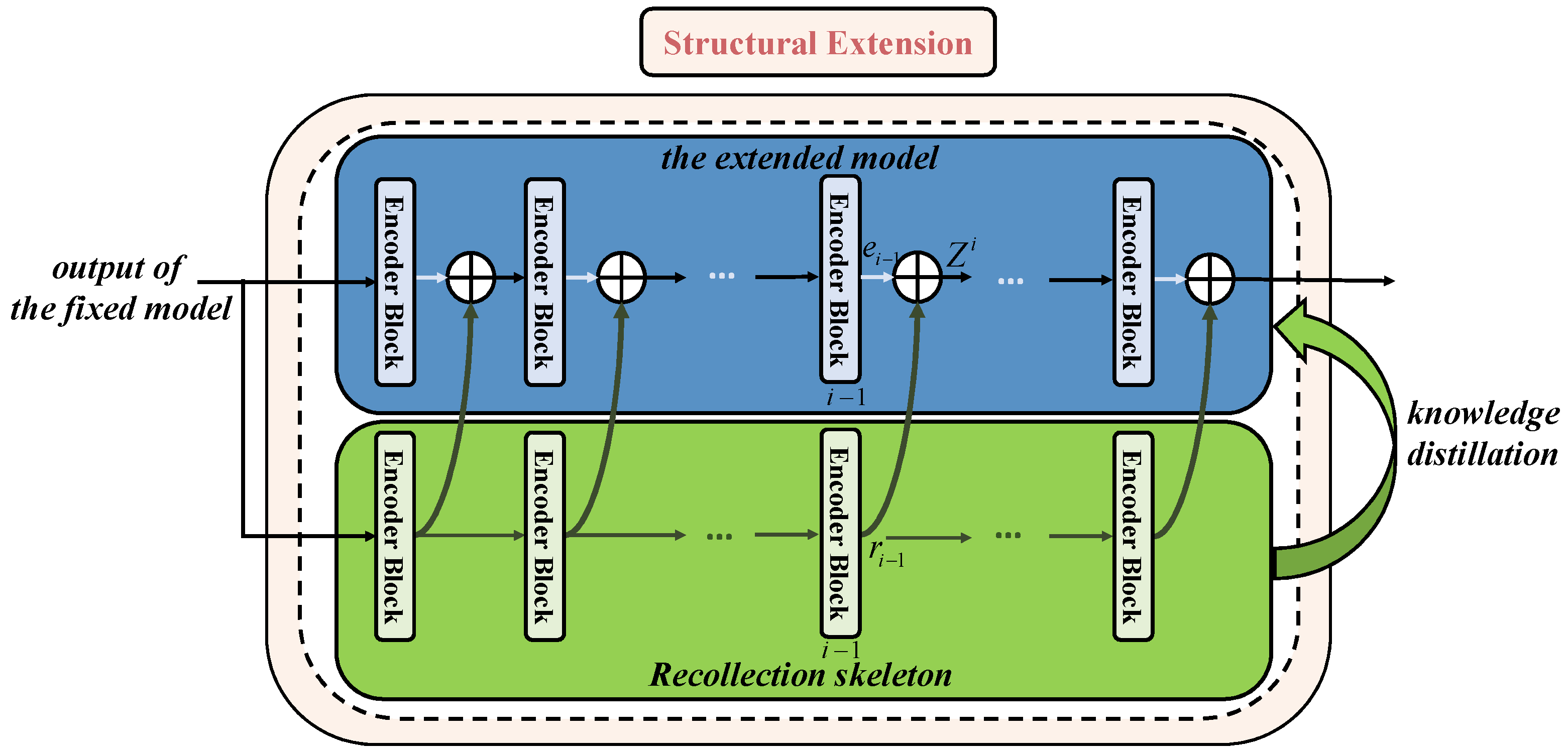
Therefore, we propose a structural extension module to imitate the learning style of the mammalian. The module consists of an extended model and a recollection skeleton structure.
As we explained in
Section 3.2, the lower layers of the model extract the basic characteristics and the higher layers extract the unique ones. Thus, the special information of classes is extracted from the higher layers of the transformer encoder module in ViT. For most of the classes, the features extracted at the lower levels are similar. The parameters of lower layers might not change dramatically when new data are added. Therefore, we froze the front
layers of the transformer encoder to extract the basic characteristics, and we use the back
layers to construct the extended model.
The recollection skeleton acts as a bridge between the past and the current. It is used to store past knowledge. When new data is put through it, the old information in the structure converts to situational memory. In order to guide the updating of the extended model with this situational memory, we propose a new embedding method. In this method, we first design the recollection skeleton to have the same structure as the extended model, and both of them consist of
encoder blocks. We then set our sights on the layers to realize information interaction. As shown in
Figure 4, every encoder block layer in the recollection skeleton embeds into the corresponding layer in the extended model. Algorithm 3 explains the process of this module.
| Algorithm 3 The process of the structural extension module |
| Input: the output of the fixed model |
Output: the output of the transformer encoder layer - 1:
for
do - 2:
Calculate the output of layer in the extended model: - 3:
Calculate the output of layer in the recollection skeleton: - 4:
Element-level summation by Equation ( 3) - 5:
- 6:
end for - 7:
return
|
The input of the structural extension module is the output of the fixed model. For the layer
i of the extended model, its input vector
is the fusion of output of layer
both in the extended model and the recollection skeleton, denoted as:
where
is the outputs of the layer
in the extended model,
is the outputs of the layer
in the recollection skeleton, ⊕ is the element-level summation of two vectors.
Because navigations that are introduced in
Section 3.3 are learnable, we take the output of the last layer corresponding to the position of navigations
as the result of the transformer encoder. This result is then averaged to obtain the feature vector
Z of the model:
At last, Z is fed to the subsequent classifier module for classification.
Before the model learns a new task, the recollection skeleton is frozen to store the parameters of the old model. When new data of the new tasks are added, the recollection skeleton structure guides the model to learn under the memories of the past. After the new tasks are added, the recollection skeleton is updated by this new data, and previous data is stored in the sample library.
It is worth noting that our model does not require the memory of the old class on the recollection skeleton to remain the same, but instead produces a memory that better fits the current stage as the new class changes. This prevents the overfitting of the model to the old class and the model can extract features that better express the properties of the new class. The structural module makes a better trade-off between plasticity and stability.
3.5. Optimizer
To achieve self-sustainment guidance representation, the optimization objectives of the model are as follows.
We use the cross-entropy loss
as the basic classification function. It determines the classification accuracy of the model and updates the model’s parameters and navigations. The cross-entropy loss denoted as:
where
y is the ground truth.
For the dynamic query navigation module, we proposed query loss function
. It denotes the difference between the keys selected by the dynamic query navigation module and the query features. It is used to update the keys. The query loss is denoted as:
where
is the cosine similarity calculation, given by Equation (
2).
For the structural extension module, we use the recollection skeleton to guide the learning of the extended model. Only using the information interaction of the structure does not positively affect the stability of the model. Therefore, we add the knowledge distillation loss to enhance the stability. The recollection skeleton acts as the teacher model to guide the extended model learning under the past information. The knowledge distillation loss is denoted as:
where
is the output of the recollection skeleton,
is the output of the extended model,
means the predicted result of the model, and
T is the temperature coefficient.
In conclusion, the loss of the base task
is defined as:
where
,
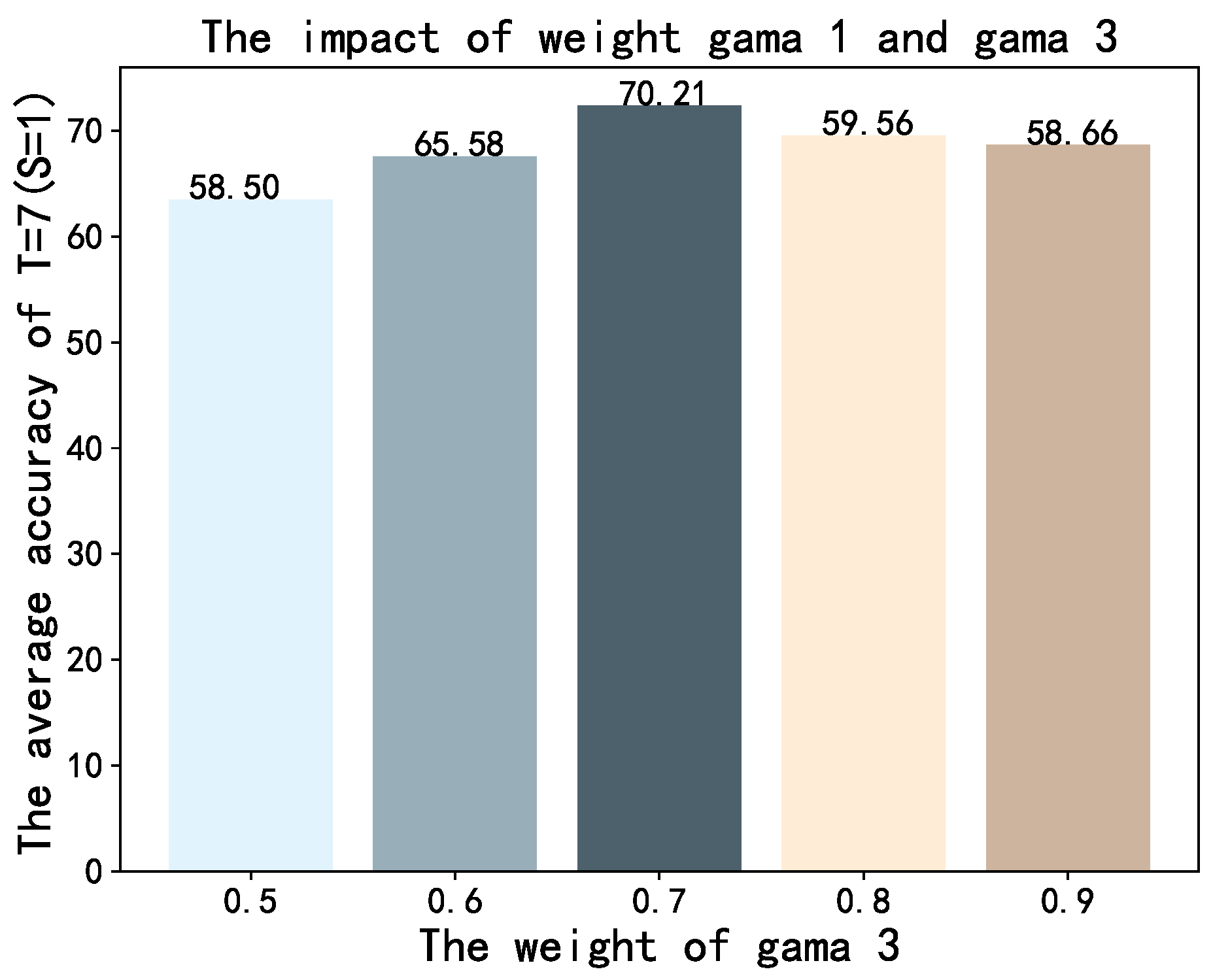
are weights.
The loss of the incremental task
is defined as:
where
,
,
are weights. According to the reference [
31], we can obtain
.


