Article

Mapping Groundwater Recharge Potential in High Latitude Landscapes Using Public Data, Remote Sensing, and Analytic Hierarchy Process

1
School of Geosciences, University of South Florida, Tampa, FL 33620, USA
2
Land Resources and Environmental Sciences, Montana State University, Bozeman, MT 59717, USA
3
Kachemak Bay National Estuarine Research Reserve, Homer, AK 99603, USA
4
Alaska Center for Conservation Science, University of Alaska, Anchorage, AK 99508, USA
*
Author to whom correspondence should be addressed.
Remote Sens. 2023, 15(10), 2630; https://doi.org/10.3390/rs15102630
Submission received: 14 April 2023 / Revised: 12 May 2023 / Accepted: 16 May 2023 / Published: 18 May 2023
(This article belongs to the Special Issue Remote Sensing Approaches to Groundwater Management and Mapping)

Abstract

:
Understanding where groundwater recharge occurs is essential for managing groundwater resources, especially source-water protection. This can be especially difficult in remote mountainous landscapes where access and data availability are limited. We developed a groundwater recharge potential (GWRP) map across such a landscape based on six readily available datasets selected through the literature review: precipitation, geology, soil texture, slope, drainage density, and land cover. We used field observations, community knowledge, and the Analytical Hierarchy Process to rank and weight the spatial datasets within the GWRP model. We found that GWRP is the highest where precipitation is relatively high, geologic deposits are coarse-grained and unconsolidated, soils are variants of sands and gravels, the terrain is flat, drainage density is low, and land cover is undeveloped. We used GIS to create a map of GWRP, determining that over 83% of this region has a moderate or greater capacity for groundwater recharge. We used two methods to validate this map and assessed it as approximately 87% accurate. This study provides an important tool to support informed groundwater management decisions in this and other similar remote mountainous landscapes.

1. Introduction

Globally, groundwater is used for agriculture (70.1%), public water supply (21.2%), and industrial activities (8.7%), thus playing a vital role in food security and human health [1,2,3,4]. Groundwater also sustains natural ecosystems. For example, it traverses natural flow paths to form and support a variety of aquatic ecosystems, such as wetlands and nearshore marine environments, and can provide a consistent discharge of water to streams and lakes [5,6,7]. However, over the past 50 years, groundwater extraction has risen dramatically, and as human populations continue to grow, groundwater consumption also increases [8].
Though essential, groundwater is also a limited resource. Its sustained availability depends on maintaining the balance between groundwater discharge and recharge [9,10]. Discharge is the expression of groundwater at the surface, often in the form of springs, some of which have been targeted for regulatory protection [11,12]. Recharge is the downward movement of water to the aquifer system, the rate of which is determined by interactions of climate, geology, topography, and land cover [13]. Recharge areas are often dispersed, less recognizable by the public, and generally lack regulatory protection as such [14]. Understanding where groundwater recharge occurs is an essential first step toward ensuring source-water protection and, therefore, groundwater supply. Multiple studies show that groundwater recharge management not only increases the groundwater supply, but when done correctly, it can raise the awareness of groundwater resources in local communities [15,16,17].
Historically, groundwater studies have relied upon field hydrogeological and geophysical measurements, geochemical tracers, and hydrologic models, depending on the questions addressed [18,19]. The accuracy of these studies depends on the scale of the analysis and the amount of data available since most methods used are data intensive [18,20,21]. Groundwater recharge studies have been performed using groundwater level data [22,23,24], sometimes integrated into water-balance models [25,26]. Physical data are often integrated with geochemical and/or isotopic data, providing further evidence to constrain groundwater recharge rates [27,28,29]. In the last decade, studies of groundwater recharge have increasingly used machine-learning algorithms [30,31]. Groundwater recharge studies that use machine learning algorithms have been successfully conducted in mid- and low-latitude regions using extensive field data and spatial datasets used for model training and testing [32,33]. However, field data collection is time-consuming and expensive, particularly inasmuch as access to field locations can be limited due to climatic extremes, rugged topography, the lack of roads, and/or land ownership. For example, exposure to extended subfreezing temperatures makes deployment and maintenance of instruments challenging in mountainous or high-latitude regions.
Increasingly, scientists have overcome these barriers by using remote sensing data and geospatial analyses to conduct groundwater studies [34,35]. This has greatly reduced the time and cost of groundwater research and enabled groundwater research even in data-poor regions [36,37]. However, many of these still require quantitative field data to define objective functions, which are then used for model training and testing [36]. Furthermore, remote sensing data come with their own challenges, as data availability and resolution (spatial and temporal) vary by region. Thus, a coherent methodology is needed to define the relative importance of remote sensing data to individual studies.
Multicriteria decision analysis (MCDA) is a methodology for organizing and assigning importance to datasets [38]. The Analytic Hierarchy Process (AHP) is the preferred MCDA technique when using geospatial data [39,40]. AHP provides a systematic methodology to classify and prioritize among heterogeneous spatial datasets and ultimately define the dataset hierarchy that best represents fundamental processes [41,42]. The coupling of these methods with GIS has made them a powerful tool for regional hydrogeologic research and decision-making.
GIS-AHP techniques can be used to address complex, multidimensional problems, such as delineating groundwater recharge zones [43,44]. The coupling of GIS and AHP techniques allows for integrating different types of data, such as in situ, remote sensing, quantitative, qualitative, or spatial data from various sources (i.e., local, regional, or global). Thus, datasets may include a range of environmental variables that cover climatic, geologic, topographic, and land cover characteristics. This versatility is critical when data are limited. When data are not readily available, and custom data acquisition is too costly or time-consuming, being able to effectively utilize common publicly available spatial data from global models, satellite imagery, and community engagement is key for knowledge development and resource management [17,21,45].
Many rural and remote areas in developed countries have incomplete or missing datasets. This data deficit has slowed the development of data-driven resource management tools. Nevertheless, many of these communities rely on groundwater for potable water and for local food production (e.g., local farms or fisheries) and require practical tools to manage these resources. In the Anchor River Watershed, south-central Alaska, a lack of comprehensive groundwater data has precluded accurate estimates of groundwater recharge to a critical aquifer system that supports local communities and connected ecosystems. As the regional population grows, consumptive use of groundwater is expected to increase, stressing this limited shared resource. Here, we used GIS, AHP, and limited remote sensing and field-derived datasets to develop and validate a groundwater recharge potential (GWRP) map in this high-latitude remote location.

2. Materials and Methods

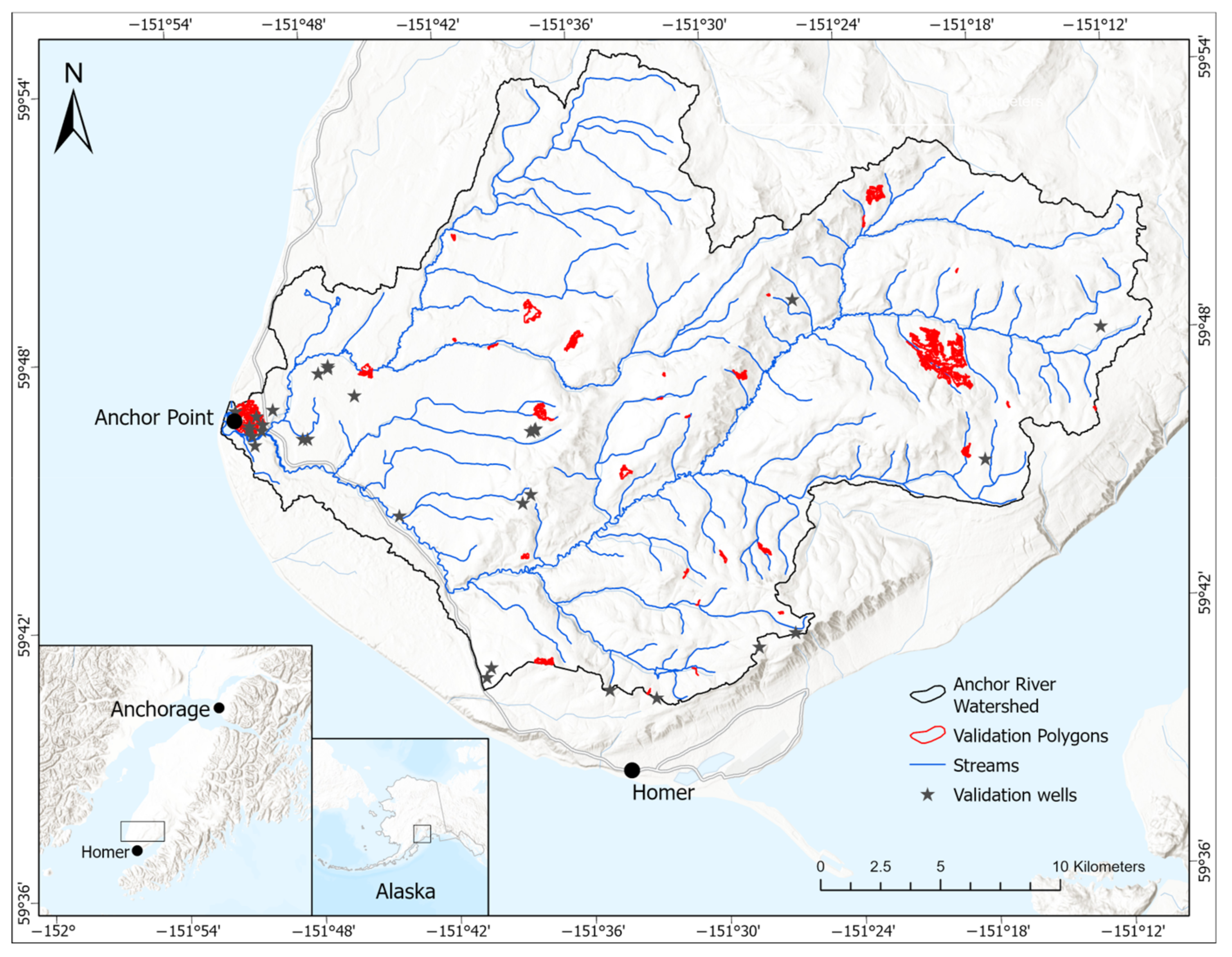
2.1. Site Description

The study area was the Anchor River Watershed on the Kenai Peninsula Lowlands in south-central Alaska (Figure 1). The Kenai Peninsula Lowlands (~9400 km2) is the unglaciated southernmost tip of the Kenai Peninsula, bordered by Kachemak Bay to the south, Cook Inlet to the west, and the Kenai Mountains range to the east. Over 40% of the Kenai Peninsula Lowlands consists of headwater streams, wetlands, and lakes [46]. The Anchor River Watershed (~586 km2) is the largest and southernmost salmon-bearing watershed on the Kenai Peninsula Lowlands. The Anchor River is a non-glacial river comprised of two main river forks that meet near the town of Anchor Point and continue west to Cook Inlet. Access to most of the watershed is challenging due to the prevalence of wetlands, streams, rugged terrain, and the lack of roads.
The climate, geology, topography, and land cover of the Anchor River Watershed are typical of the Kenai Peninsula Lowlands. The climate is driven by continental and maritime patterns, from north to south, and consists of short summers and long cold winters. Mean annual temperature and precipitation are 2.9 °C and 755.14 mm, respectively (HOMER 8 NW, AK US USC00503672, 1991–2020). Seasonal precipitation is influenced by the strength and position of the Aleutian Low, with most of the precipitation occurring between November and March [47], with the orographic effects of the bordering mountains creating distinctive climatic zonation [48]. The region has experienced at least five major glaciations and two minor glacial advances over the last 125,000 years [48]. Geologic deposits are a complex mix of Pleistocene glacial deposits overlaying weakly lithified Tertiary bedrock [48,49,50]. Groundwater can be found in all deposits, most notably in the Pleistocene glacial deposits, especially in valley train and outwash channel deposits [36,51]. Relief is rugged and steep, with total relief ranging from 0 m to 621 m above mean sea level (AMSL).
The water resources availability and patterns of use in the Anchor River Watershed are also typical of the Kenai Peninsula Lowlands. People rely almost exclusively on groundwater for domestic, commercial, and industrial uses [52], but there are few statewide or local restrictions on groundwater use. Wherever water occurs naturally in Alaska, it is a common property resource, not attached to land ownership unless the landowner applies for a water right [53]. Similarly, ecosystems rely on groundwater, notably salmon-bearing streams. Groundwater augments streamflow [54] and may provide >50% of the streamflow during spring breakup and fall freshets and >80% of the streamflow during late summer and throughout the winter (Brigino, unpublished data). In many cases, aquifers used for water supply are the same aquifers that outcrop on hillslopes and support seeps and springs that discharge to the streams [36,55]. The balance is delicate because the shared aquifer resources are largely glacial channel and floodplain deposits that are multitiered, thin, discontinuous, and prone to drawdown and drying [52].
The largest municipality in the region is the City of Homer, which has a population of ~6000 people and has seen a population increase of 10% since the 2010 census [56]. Although the City of Homer is not entirely located within the Anchor River Watershed, the source of the City’s drinking water (Bridge Creek Reservoir) is in the headwaters. Natural tracer studies indicate that >50% of the water in the Bridge Creek Reservoir originates from groundwater discharging from seeps and springs (Brigino, unpublished data). This reservoir not only serves the City of Homer but also provides drinking water to people that live in the region. The only other potable water sources are private or public groundwater wells and naturally flowing springs.

2.2. Overall Approach

Our study included four stages to develop a spatial model to delineate GWRP zones: (1) develop a conceptual model, (2) select and process spatial datasets, (3) rank spatial datasets and their corresponding classes, (4) create and validate a GIS-based map of GWRP. We used ArcGIS Pro 2.9.2 (ESRI, Redlands, CA, USA), QGIS 3.22 Biatowieza (QGIS Development Team (2022)), and the Soil & Water Assessment Tool+ (SWAT+) (USDA-ARS) to process and analyze our spatial datasets.

2.3. Conceptual Model Development

Our conceptual model of groundwater resources in our study area was developed over many field seasons [36,54,55,57], but most specifically during three visits in 2018–2019 and 2021–2022. During these visits, we initially focused on using remote sensing data and machine learning to locate the seeps and springs that discharge groundwater to the salmon-bearing streams [36]. In the Kenai Peninsula Lowlands, groundwater discharge in one location implies groundwater recharge in another, likely nearby and upgradient. Therefore, we simultaneously made field observations about areas that likely supported groundwater recharge, focusing on evidence that could be derived from publicly available data (e.g., climate, geology, soils, topography, and land cover). We simultaneously incorporated community insights, including indigenous tribal knowledge, through surveys and interviews (Guerrón-Orejuela, unpublished data) [55]. We used the conceptual model developed from these field observations and community knowledge to identify and rank the spatial datasets and criteria that drive groundwater recharge.

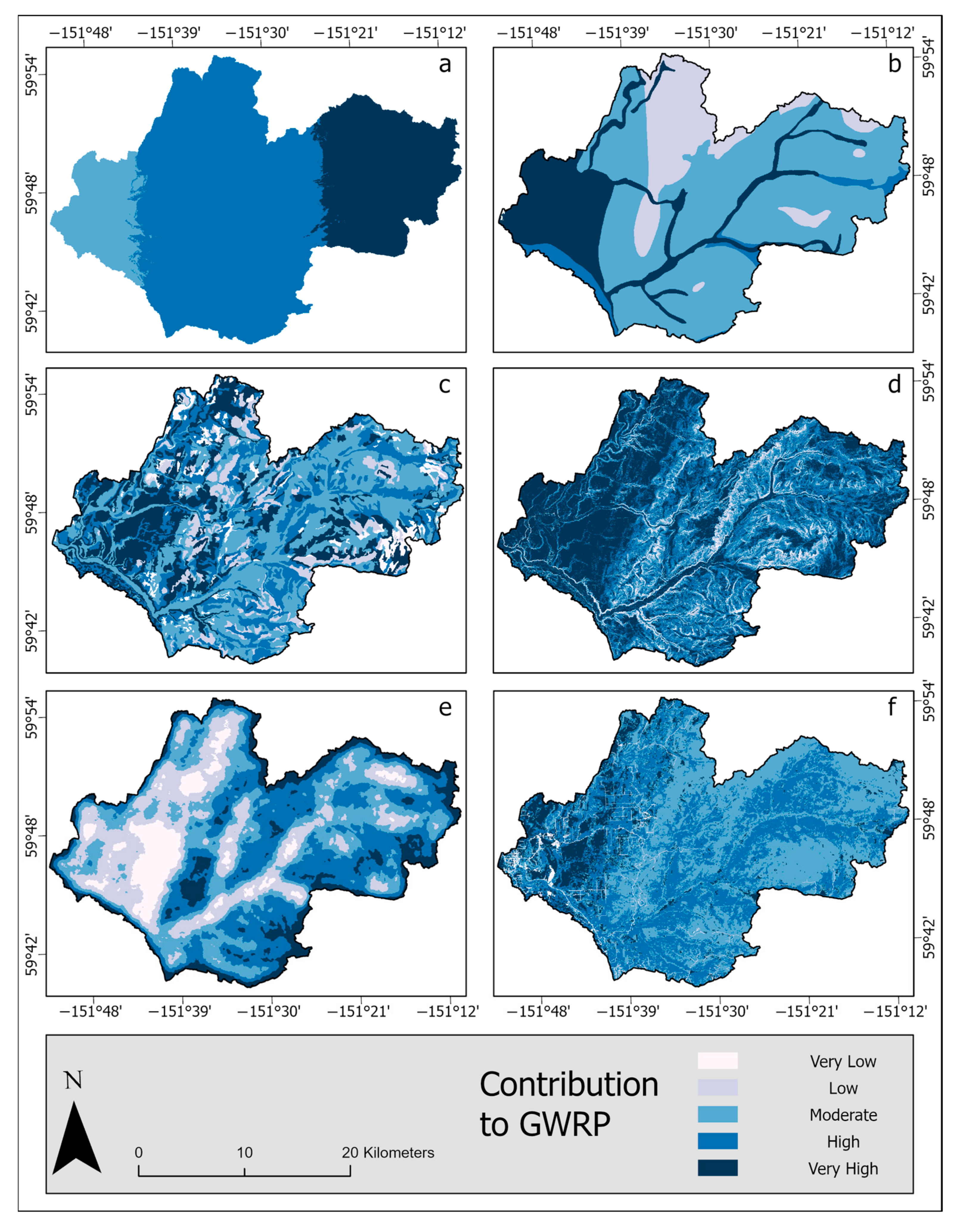
2.4. Spatial Dataset Selection

We performed a literature review of twenty-three geospatial groundwater potential and groundwater recharge potential studies to crowdsource possible criteria and supporting spatial datasets [21,40,43,58,59,60,61,62,63,64,65,66,67,68,69,70,71,72,73,74,75,76,77]. Detailed results, including spatial datasets organized by reference, are supplied in Supplementary Materials Table S1. These studies used different quantities and types of spatial datasets, ranging from 5 to 13, typically picked from climatic, geologic, topographic, and land cover data sources. Our analysis showed twenty-eight unique spatial datasets used in all the studies. Eleven were only used in one study, and eight were used at least two times more than any other. These eight common spatial datasets are precipitation, geology, lineament density, soils, geomorphology, slope, drainage density, and land use and land cover (Figure 2).
We were interested in developing a methodology with a high likelihood of being available and applicable to various regions. Therefore, we chose to work with the spatial datasets our literature review revealed were exceptionally common in groundwater studies. Of the eight spatial datasets presented above, six spatial datasets or the related underlying data that collectively represented climatic, geologic, topographic, and land cover characteristics were available for our study area: precipitation (P), geology (G), soil texture (ST), slope (SL), drainage density (DD), and land cover (LC). The remaining two, lineaments and geomorphology, were unavailable. All layers used in the analysis were standardized to 3 × 3 m.
We represented climate through spatially distributed precipitation data, some fraction of which would be available for groundwater recharge [78,79]. Precipitation data were limited in our study area, so we generated a spatially distributed dataset based on data from twenty available weather stations in our region using the weather generator in the SWAT + modeling software [80]. This software uses the global weather station network and data derived from satellite products (Climate Forecast System Reanalysis (CFSR), National Center for Environmental Prediction) [81].
We represented geology through spatially distributed lithology and soils, which affect infiltration [82,83,84,85]. We derived lithology data from the United States Geological Survey (USGS) Geologic map of Alaska [86], which is a compilation of regional geologic maps developed and published by the USGS National Survey and Analysis Project for Alaska. We used the lithologic coding to query and identify the most specific part of the lithologic assignment available for our study area. The resulting vector file was rasterized. For soils, we used the National Resources Conservation Service’s (NRCS) gridded (10 m resolution) Soil Survey Geographic Database (gSSURGO) for the State of Alaska [87]. From these data, we extracted soil texture, which is proportional to permeability [88].
We represented topography through a digital elevation model (DEM), which represented the likelihood of precipitation runoff [89,90]. Topographic data were derived from airborne LiDAR (2008 Kenai Watershed Forum Topographic LiDAR: Kenai Peninsula, Alaska; https://www.fisheries.noaa.gov/inport/item/49620; accessed on 25 February 2019). The LiDAR-based digital elevation model (DEM) was acquired at 1 × 1 m pixel size but was resampled to a 3 × 3 m pixel size, which reduced run times and microtopographic anomalies [36]. Topographic data directly extracted from the DEM included slope and drainage density [91,92]. Additionally, this DEM was used to delineate the study area using Arc Hydro Pro tools.
We used the most up-to-date land cover data for this region, representing the degree to which development altered the natural landscape, especially by placing impervious surfaces [93,94]. We derived our grid (30 m spatial resolution) from the 2016 National Land Cover Database (NLCD) [95].

2.5. Spatial Dataset Weighting through Analytic Hierarchy Process (AHP)

We used AHP, and Saaty’s relative importance scale, to assess and compare the relative contribution to groundwater recharge of the data represented in the six spatial datasets. In Saaty’s relative importance scale, 1 indicates equal importance between classes, and 9 shows the extreme importance of one class above another (Table 1).
To determine the weights of each spatial dataset, we constructed a 6 × 6 pairwise comparison matrix (1), where each element a ij was evaluated based on our conceptual model. To fill out the matrix, we conducted pairwise comparisons of each of the six spatial datasets, assigning high relative importance values to spatial datasets that greatly influence groundwater recharge and low relative importance values to those with a small impact on groundwater recharge [41,43,76]. Only comparisons above the matrix diagonal (1) are required.
A = 1 a 12 a 1 n a 21 1 a 2 n a n 1 a n 2 1
Elements below the diagonal were assigned reciprocal values of the corresponding above-diagonal values [41], as represented in Equation (2).
a i j = 1 a j i
According to the AHP methodology, the principal eigenvector, p , is the desired priorities vector. We approximated p by normalizing the elements in each column of the comparison matrix and then averaging over each row [41]. We estimated λ m a x by adding the columns of A and multiplying the resulting vector by p . The difference between λ m a x and the number of spatial datasets (n) is a measure of the inconsistency of the comparison matrix. We calculated the consistency index (CI) as per Equation (3) [41], where CI is the consistency index, n is the number of spatial datasets, and λ m a x is the largest eigenvalue.
C I = λ m a x n   n 1
We also used the random consistency index (RI), a table-based value dependent on the number of variables used, to calculate the consistency of the comparison matrix, which is a measure of how far the comparison matrix is from total consistency [42,96]. For our analysis n = 6, which corresponds to RI = 1.24 (Table 2).
Finally, we calculated the consistency ratio (4), which measures the consistency of the judgment used during the pairwise comparison based on transitive property.
C R = C I R I .
Each spatial dataset contains information in classes. The information contained in these classes can be quantitative or qualitative. For this study, we used spatial datasets with classes determined by both. For example, in our study area, the land cover dataset consists of 15 land cover classes, and the slope dataset has slope values ranging from 0% to >60%. We used the natural breaks classification method (Arc Pro v 2.9.2, ESRI) to rank the classes within the quantitative spatial datasets (precipitation, slope, and drainage density) [43], thus maximizing differences between classes. We used our conceptual model to assign ranks for classes within qualitative spatial datasets (geology, soil texture, and land cover). The final class ranking values were based on Saaty’s relative importance scale (see Table 1).

2.6. GWRP Model Development and Validation

We used the weighted overlay tool (Arc Pro v 2.9.2, ESRI) to combine the six spatial datasets into a single map. Then, we assigned the corresponding normalized principal eigenvector value to each spatial dataset and reclassified the results using natural breaks classification. The GWRP zones were classified into five categories: Very Low, Low, Moderate, High, and Very High.
We used two methods to validate the GWRP model. In the first validation, two experts with local knowledge conducted an independent assessment of 30 randomly chosen GWRP polygons that the model had scored as GWRP = high or GWRP = low. The experts did not have access to the scores assigned by the model but did have access to the unprocessed layers used in the model (as downloaded from the web). They also had access to ancillary information not used directly in the model, such as well-logs, aquifer outcrops, topographic wetness index (TWI), flow-weighted slope (FWS), terrain ruggedness index (TRI), and planform and profile curvature [36]. In the second validation, we determined whether wells in areas with higher GWRP scores were more likely to have higher well yields than wells in areas with lower GWRP. We obtained well yield information from well logs publicly available in the Well Log Tracking System (WELTS) (https://dnr.alaska.gov/welts/; accessed on 2 December 2022). From over 200 wells, we randomly selected 30 wells located in areas that the model had scored as GWRP = high or GWRP = low. Then, we performed a Mann–Whitney U test on the well yield data from these 30 wells to determine if well yields reported in the two populations were significantly different. We used the receiver operating characteristic curve (ROC) and the area under the curve (AUC) to determine the accuracy of the model using this second validation method [97,98].

3. Results

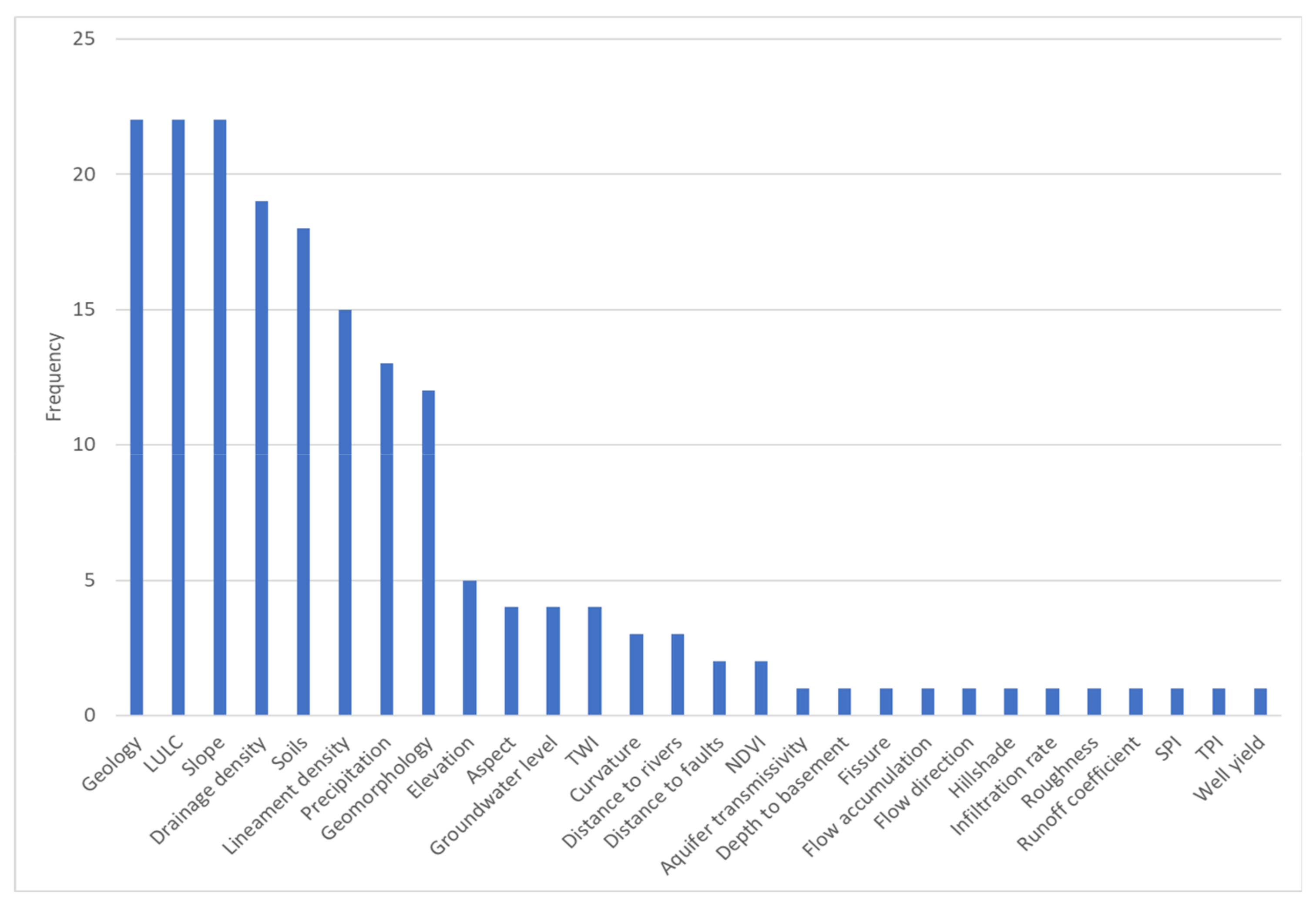
3.1. Relative Ranking of Individual Spatial Datasets

The spatial dataset weighting procedures resulted in a normalized reciprocal matrix with principal eigenvectors and the largest eigenvalues for each spatial dataset (Table 3). The value of the principal eigenvector reflects the relative influence of each spatial dataset on the GWRP model. Slope has the greatest influence on GWRP, with a weight of 33%. Land cover, soil texture, precipitation, and geology have the subsequent greatest influence on GWRP, with weights of 22%, 17%, 12%, and 11%, respectively. Drainage density has the least influence on GWRP, with a weight of just 4% (Table 3, principal eigenvector). The consistency ratio for the reciprocal matrix is 0.04. Consistency ratios of 0.10 or less have been deemed acceptable [41].

3.2. Relative Ranking of Data Classes within Spatial Datasets

The spatial dataset selection procedures resulted in six spatial datasets, with data reclassified in terms of their relative contribution to GWRP (Table 4; Figure 3; Supplementary Materials Tables S2–S7). GWRP is highest where precipitation is relatively high, coarse-grained, unconsolidated deposits are present, soils are variants of sands and gravels, the terrain is flat, the drainage density is low, and there is no development. Conversely, GWRP is lowest where precipitation is relatively low, tertiary sedimentary rock is present, soils have very high organic matter content, the terrain is steep, the drainage density is high, and there is high-density development.

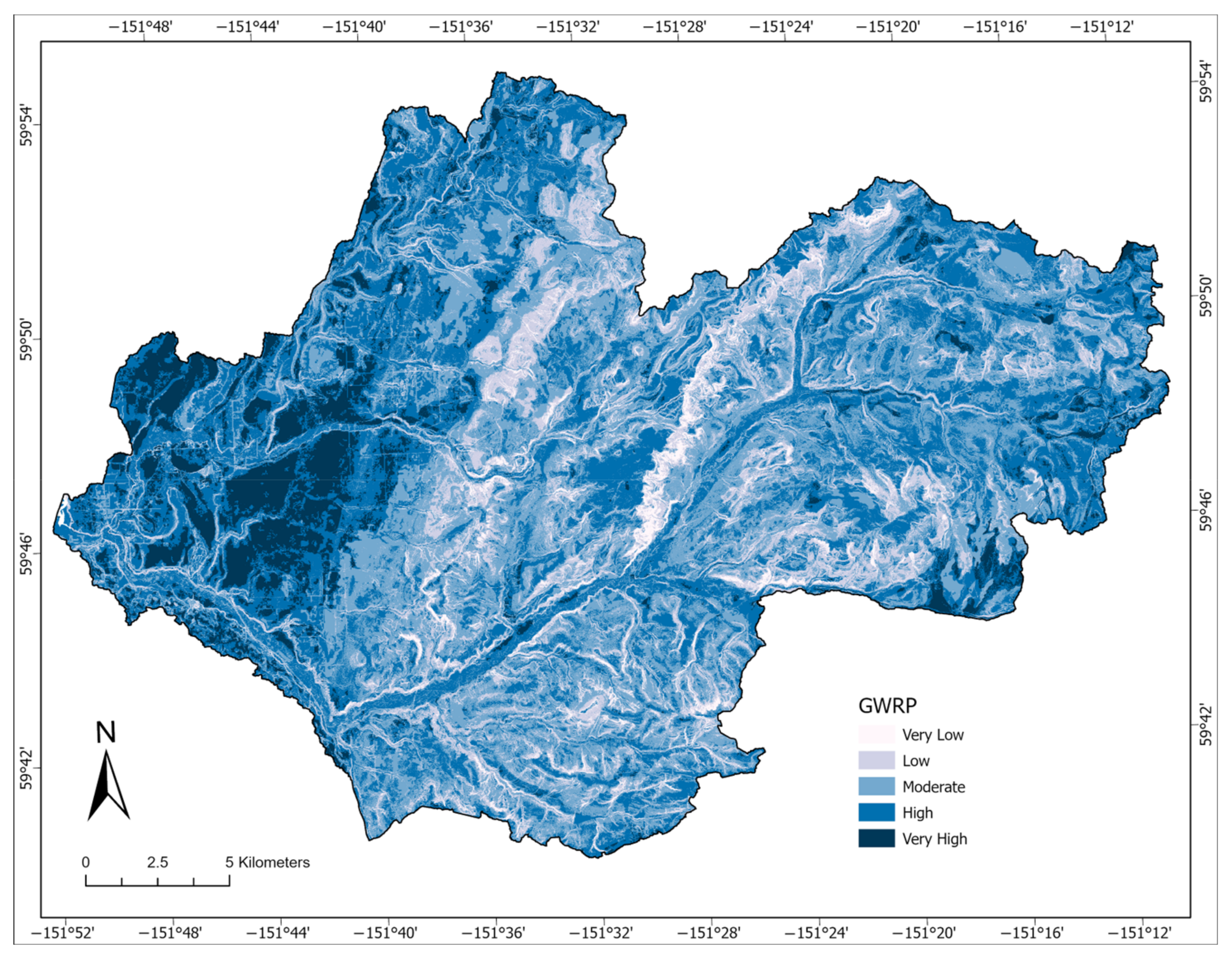
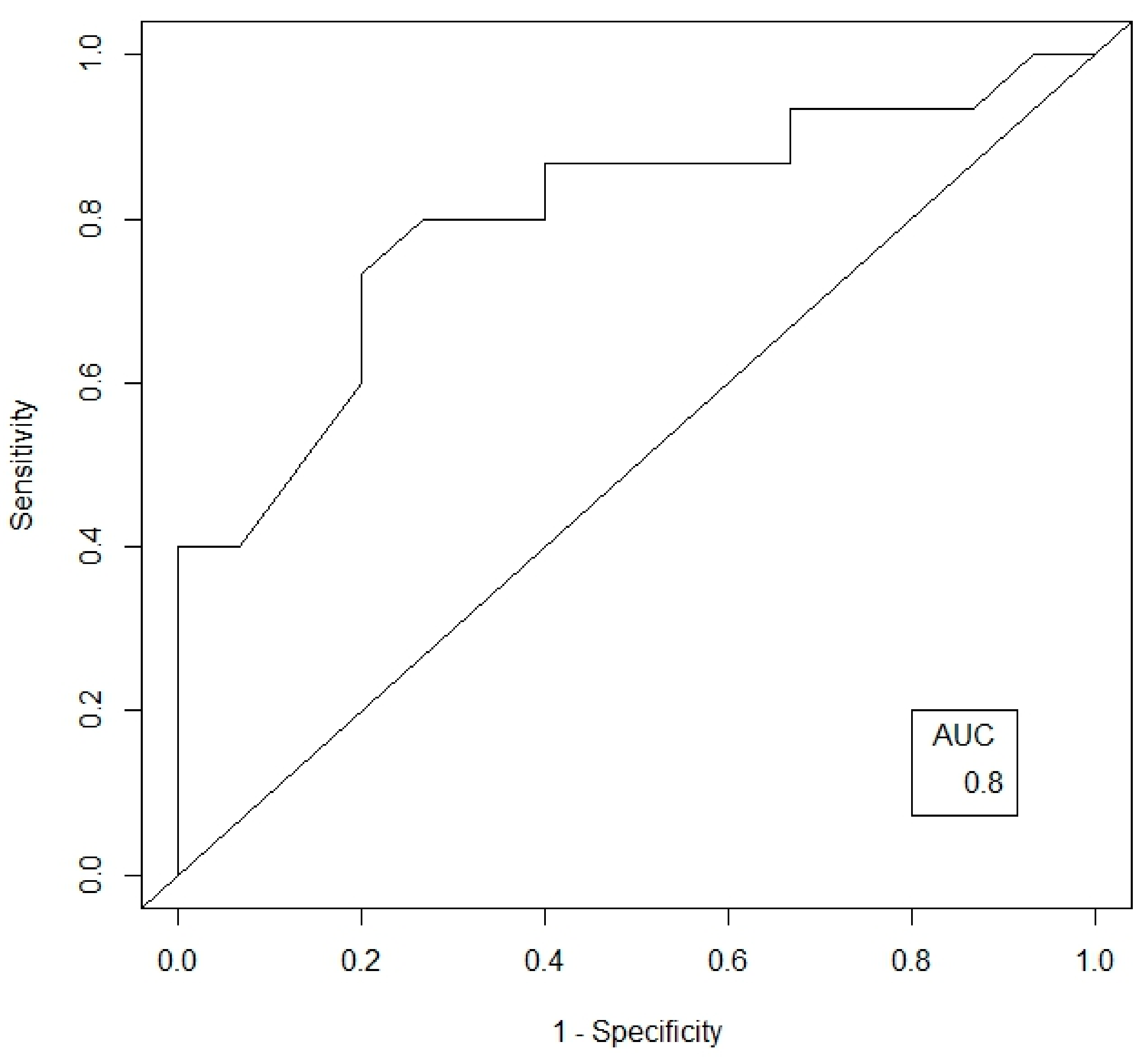
3.3. GWRP Model and Validation

The GWRP model reveals that groundwater recharge potential is not uniformly distributed across the landscape, dividing the watershed into five GWRP zones: Very Low, Low, Moderate, High, and Very High (Figure 4). From the total area of our study area, 3% has Very Low GWRP, 14% has Low GWRP, 39% has Moderate GWRP, 36% has High GWRP, and 8% has Very High GWRP. Overall, 83% of the watershed is at least moderately suitable for groundwater recharge.
We built a confusion matrix to summarize and evaluate our expert-based validation results (Table 5). Our expert-based model validation showed a high concurrency between the GWRP model and expert assignments, with an overall accuracy, sensitivity, and precision of 87%.
In addition to the expert-based model validation, we compared well yields from 30 wells, equally divided between locations where GWRP values are Low and High. Median well yields for areas where GWRP values are Low and High were 18.9 L per minute and 37.9 L per minute, respectively. The well yields reported in each group were not normally distributed, so we conducted a Mann–Whitney U test and determined the accuracy of the model by calculating the receiver operating characteristic curve (ROC) and the area under the curve (AUC) (Figure 5).
The results indicate that the well yields in locations with low GWRP values were significantly lower than those in areas with high GWRP values (Mann–Whitney U = 41, n1 = n2 = 15, p < 0.05 two-tailed). The findings of the ROC analysis indicate that the AUC was 0.8, and the model is, therefore, 80% accurate.

4. Discussion

This GWRP model reveals that groundwater recharge potential in the study area is driven primarily by slope, then by land cover, soil texture, precipitation, geology, and drainage density, in that order. Each of these plays a crucial role, so the overall variability in GWRP is a function of variables with both high spatial variability (e.g., slope, soil texture) and low spatial variability (e.g., precipitation, land cover) (Figure 3). Specifically, areas where GWRP values are highest are relatively low gradients and have relatively high-permeable surficial deposits and relatively high precipitation, and largely natural land cover. These areas are not distributed uniformly throughout our study area (Figure 4). The model shows that groundwater recharges mainly in proglacial lake bottom sediments underlying terraced and channeled surfaces between major morainal belts in lowland and mountain valleys, as well as in flood plains and associated higher terraces along major streams and abandoned drainage lines.
The distribution of GWRP zones concurs with other studies conducted in mountainous regions. Areas with steep slopes and shallow bedrock typically have GWRP values of Very Low and Low [73,76,77]. Conversely, areas along streams and floodplains, valley bottoms, and other flat areas with alluvium commonly have GWRP values of High and Very High [62,64,73]. Similarly, field groundwater studies have indicated that groundwater recharge in mountainous areas is spatially variable [79]. Areas with high recharge often are characterized by high precipitation [78], undeveloped landscape [93], and flat alluvial fans as the main geologic feature [83,89].
Our results demonstrate that a large percentage of this landscape is engaged in groundwater recharge at moderate or higher levels, cumulatively contributing to groundwater supply. Independent measurements of total groundwater recharge are unavailable in the study area. However, total groundwater recharge nearby and in similar terrain was approximately 0.19 cm/d in June–September, mostly through closed-basin depressions [26]. An independent estimate of net annual groundwater recharge in the study area suggests volumes of approximately 1% of annual precipitation (M. Rains, unpublished data). Net groundwater recharge is expected to be much lower than total recharge in this area as most of this groundwater recharge is subsequently either extracted by wells [52] or discharged from the numerous seeps and springs (M. Rains, unpublished data) [36]. The maintenance of the total groundwater recharge is crucial because it supports both these communities and these water-dependent ecosystems.
Groundwater is the region’s primary source of domestic, commercial, and industrial water supply [52]. People source their domestic drinking water from private and public wells, springs, or the Bridge Creek Reservoir operated by the City of Homer. Although the Bridge Creek Reservoir is a surface-water reservoir, >50% of this water originates from nearby seeps and springs (Brigino, unpublished data). Meanwhile, groundwater discharge from seeps and springs also supports streamflow (Brigino, unpublished data) [54], modulates stream temperatures, providing cool-water refugia in summer and warm-water refugia in winter [54], and delivers nutrient subsidies to the streamside wetlands and streams, mainly from hillslopes covered with N-fixing alders [57,100]. Overall, these groundwater subsidies are crucial to the proper functioning of streams, including the streamside wetlands [57,101], the benthos [102], and the salmonids [103]. Groundwater is the central link between all these processes, with the salmonids being notable beneficiaries.
GWRP maps are important tools for increasing awareness and enabling effective management of groundwater resources, especially source-water protection. To our knowledge, most previous studies that couple GIS and AHP to delineate GWRP have been conducted in low and middle-latitude regions, often in dry climatic regions and in less economically developed nations [59,61,68]. However, many communities in high latitudes, including in wetter regions and in more economically developed nations, are similarly dependent on groundwater and similarly limited by data. Here, we used GIS and AHP to construct a GWRP map in a remote, high-latitude region based on remote sensing data and on a conceptual model developed from a combination of field observations and community engagement.
Our model incorporated high-quality data and insights provided by field experience, as available. Acquiring such data is often a challenge, especially in high-latitude regions. We overcame this by performing a literature review and crowdsourcing eight possible criteria and supporting spatial datasets [21,40,43,58,59,60,61,62,63,64,65,66,67,68,69,70,71,72,73,74,75,76,77], then eliminating two criteria and datasets that were unavailable for our study area (Figure 2). This ensured we only considered widely available criteria and datasets, which are likely to also be available elsewhere. We benefitted from the availability of a LiDAR-derived DEM with a resolution of 1 × 1 m, which we resampled to a resolution of 3 × 3 m. The resolution of this DEM is likely higher than will be available in many other remote regions, which might only have DEMs with a much lower resolution (e.g., Landsat Collection 2 Digital Elevation Model, https://www.usgs.gov/landsat-missions/landsat-collection-2-digital-elevation-model, accessed on 10 May 2023). We chose to use our higher resolution DEM because it better represented the rugged topography which played such a crucial role in our study area (see Slope in Figure 3). Though many other high-latitude regions may not have similar higher-resolution DEMs, we note that higher-resolution DEMs are rapidly becoming more widely available (e.g., 1 m Digital Elevation Models (DEMs)—USGS National Map 3DEP Downloadable Data Collection, https://data.usgs.gov/datacatalog/, accessed on 10 May 2023).
Combining AHP with powerful spatial and statistical analysis within a GIS environment creates a valuable tool for water resources management. This method allows qualitative and quantitative criteria to be considered in decision-making. AHP’s biggest weakness is the potential for evaluator bias when establishing criteria and developing the pairwise comparison matrix. We overcame this weakness by combining community engagement and fieldwork expertise. Past community engagement [55] and recent surveys and interviews (Guerrón-Orejuela, unpublished data) identified community interest in geospatial information regarding groundwater recharge and assessed community understanding of regional hydrological patterns and processes. Fieldwork provided an improved understanding of the drivers of regional hydrological patterns and processes, especially as they relate to groundwater discharge to streams [54,57] and the structure of regional aquifers that support both water supply and springs [36]. This effectively crowdsourced the spatial datasets and weights.
For the past three decades, scientists and resource managers in the Kenai Peninsula Lowlands have become increasingly aware of the need to understand ecological processes to sustain a healthy and resilient community, especially in this low-regulatory setting that is facing an increasing population, changes in climactic conditions, and potential reduction of vital resources. It has become clear that scientists need to create tools to effectively communicate science to stakeholders, thus facilitating communication and allowing for better and informed local decision-making [55]. This GWRP map can serve in that capacity, guiding land and resource management decisions by identifying recharge areas. Furthermore, given the community’s reliance on groundwater as their primary source of potable water, this model provides important information regarding source-water protection. This tool joins an ever-growing list of tools that empower local communities to have an informed dialog about how to manage the landscape best to reduce the risk of groundwater depletion. Finally, our study refines techniques, extends them to a new region, and provides insights critical for management regarding where groundwater recharge occurs in this and other similar landscapes.

Supplementary Materials

The following supporting information can be downloaded at: https://www.mdpi.com/article/10.3390/rs15102630/s1, Table S1: Literature review of possible criteria and supporting spatial datasets; Table S2: Precipitation classes contribution to Groundwater Recharge Potential (GWRP); Table S3: Geology classes contribution to Groundwater Recharge Potential (GWRP), Table S4: Soil Texture classes contribution to Groundwater Recharge Potential (GWRP); Table S5: Slope classes contribution to Groundwater Recharge Potential (GWRP); Table S6: Drainage Density classes contribution to Groundwater Recharge Potential (GWRP); Table S7: Land Cover classes contribution to Groundwater Recharge Potential (GWRP).

Author Contributions

This manuscript is the result of a broad, collaborative effort by all authors. Conceptualization, M.C.R., C.M.W. and E.J.G.-O.; methodology, E.J.G.-O., K.C.R. and M.C.R.; validation, E.J.G.-O., K.C.R. and M.C.R.; formal analysis, E.J.G.-O.; investigation, E.J.G.-O., K.CR., T.M.B., C.M.W. and M.C.R.; data curation, E.J.G.-O.; writing—original draft preparation, E.J.G.-O., K.C.R. and M.C.R.; writing—review and editing, E.J.G.-O., K.C.R., T.M.B., W.J.K., S.M.L., P.S., C.M.W. and M.C.R.; visualization, E.J.G.-O.; supervision, K.C.R. and M.C.R.; project administration, E.J.G.-O., K.C.R., C.M.W. and M.C.R.; funding acquisition, E.J.G.-O., K.C.R., C.M.W. and M.C.R. All authors have read and agreed to the published version of the manuscript.

Funding

This research was funded primarily by the NOAA Office of Coastal Management Margaret A. Davidson Graduate Fellowship, Federal Award Number NA20NOS4200143, and the National Estuarine Research Reserve System Science Collaborative under Grant No. 54584 (https://nerrssciencecollaborative.org/project/Walker17, accessed on 10 May 2023). Additional funding was provided by the University of South Florida School of Geosciences’ Fred L. and Helen M. Tharp Endowed Scholarship. The APC was funded by the Ecohydrology Lab at the University of South Florida.

Data Availability Statement

Publicly available datasets were analyzed in this study. This data can be found here:, https://doi.org/10.6084/m9.figshare.22589185.v1, accessed on 15 May 2023.

Acknowledgments

This project benefitted immeasurably from in-kind support provided by the Kachemak Bay National Estuarine Research Reserve, which provided lodging, local knowledge, introductions to stakeholders, the coordination of formal stakeholder engagements, and more. Syverine Bentz was particularly instrumental. A special thank you to all the many stakeholders who provided their time and local knowledge. We would also like to acknowledge the anonymous reviewers for their constructive comments.

Conflicts of Interest

The authors declare no conflict of interest. The funders had no role in the design of the study; in the collection, analyses, or interpretation of data; in the writing of the manuscript; or in the decision to publish the results.

References

  1. de Graaf, I.E.M.; Gleeson, T.; van Beek, L.P.H.R.; Sutanudjaja, E.H.; Bierkens, M.F.P. Environmental Flow Limits to Global Groundwater Pumping. Nature 2019, 574, 90–94. [Google Scholar] [CrossRef] [PubMed]
  2. Forslund, A.; Renöfält, B.M.; Barchiesi, S.; Cross, K.; Davidson, S.; Farrel, T.; Korsgaard, L.; Krchnak, K.; McClain, M.; Meijer, K.; et al. Securing Water for Ecosystems and Human Well-Being the Importance of Environmental Flows; Stockholm International Water Institute (SIWI): Stockholm, Sweden, 2009. [Google Scholar]
  3. Margat, J.; van der Gun, J. Groundwater around the World: A Geographic Synopsis; CRC Press: Boca Raton, FL, USA, 2013; ISBN 978-1-138-00034-6. [Google Scholar]
  4. United Nations. The United Nations World Water Development Report 2022: Groundwater: Making the Invisible Visible; UNESCO: Paris, France, 2022; ISBN 978-92-3-100507-7. [Google Scholar]
  5. Winter, T.C. Relation of Streams, Lakes, and Wetlands to Groundwater Flow Systems. Hydrogeol. J. 1999, 7, 28–45. [Google Scholar] [CrossRef]
  6. Hood, J.L.; Roy, J.W.; Hayashi, M. Importance of Groundwater in the Water Balance of an Alpine Headwater Lake. Geophys. Res. Lett. 2006, 33, L13405. [Google Scholar] [CrossRef]
  7. Callegary, J.B.; Kikuchi, C.P.; Koch, J.C.; Lilly, M.R.; Leake, S.A. Review: Groundwater in Alaska (USA). Hydrogeol. J. 2013, 21, 25–39. [Google Scholar] [CrossRef]
  8. Boretti, A.; Rosa, L. Reassessing the Projections of the World Water Development Report. NPJ Clean Water 2019, 2, 15. [Google Scholar] [CrossRef]
  9. Baldwin, H.L.; McGuinness, C.L. A Primer on Ground Water; General Interest Publication; 1990 reprint; U.S. Geological Survey: Washington, DC, USA, 1963; p. 31.
  10. Famiglietti, J.S. The Global Groundwater Crisis. Nat. Clim. Chang. 2014, 4, 945–948. [Google Scholar] [CrossRef]
  11. Alfaro, C.; Wallace, M. Origin and Classification of Springs and Historical Review with Current Applications. Environ. Geol. 1994, 24, 112–124. [Google Scholar] [CrossRef]
  12. Gannon, C. Legal Protection for Groundwater-Dependent Ecosystems. MJEAL 2014, 4, 183. [Google Scholar] [CrossRef]
  13. de Vries, J.J.; Simmers, I. Groundwater Recharge: An Overview of Processes and Challenges. Hydrogeol. J. 2002, 10, 5–17. [Google Scholar] [CrossRef]
  14. Owen, D. Law, Land Use, and Groundwater Recharge. Stanf. Law Rev. 2021, 73, 1173. [Google Scholar] [CrossRef]
  15. Cruz-Ayala, M.B.; Megdal, S.B. An Overview of Managed Aquifer Recharge in Mexico and Its Legal Framework. Water 2020, 12, 474. [Google Scholar] [CrossRef]
  16. Dillon, P. Future Management of Aquifer Recharge. Hydrogeol. J. 2005, 13, 313–316. [Google Scholar] [CrossRef]
  17. Jadeja, Y.; Maheshwari, B.; Packham, R.; Bohra, H.; Purohit, R.; Thaker, B.; Dillon, P.; Oza, S.; Dave, S.; Soni, P.; et al. Managing Aquifer Recharge and Sustaining Groundwater Use: Developing a Capacity Building Program for Creating Local Groundwater Champions. Sustain. Water Resour. Manag. 2018, 4, 317–329. [Google Scholar] [CrossRef]
  18. Scanlon, B.R.; Healy, R.W.; Cook, P.G. Choosing Appropriate Techniques for Quantifying Groundwater Recharge. Hydrogeol. J. 2002, 10, 18–39. [Google Scholar] [CrossRef]
  19. Tóth, J. A Theoretical Analysis of Groundwater Flow in Small Drainage Basins. J. Geophys. Res. 1963, 68, 4795–4812. [Google Scholar] [CrossRef]
  20. Huet, M.; Chesnaux, R.; Boucher, M.-A.; Poirier, C. Comparing Various Approaches for Assessing Groundwater Recharge at a Regional Scale in the Canadian Shield. Hydrol. Sci. J. 2016, 61, 2267–2283. [Google Scholar] [CrossRef]
  21. Jaafarzadeh, M.S.; Tahmasebipour, N.; Haghizadeh, A.; Pourghasemi, H.R.; Rouhani, H. Groundwater Recharge Potential Zonation Using an Ensemble of Machine Learning and Bivariate Statistical Models. Sci. Rep. 2021, 11, 5587. [Google Scholar] [CrossRef]
  22. Meyboom, P. Unsteady Groundwater Flow near a Willow Ring in Hummocky Moraine. J. Hydrol. 1966, 4, 38–62. [Google Scholar] [CrossRef]
  23. Johansson, P.-O. Estimation of Groundwater Recharge in Sandy till with Two Different Methods Using Groundwater Level Fluctuations. J. Hydrol. 1987, 90, 183–198. [Google Scholar] [CrossRef]
  24. van der Kamp, G.; Hayashi, M. The Groundwater Recharge Function of Small Wetlands in the Semi-Arid Northern Prairies. Great Plains Res. J. Nat. Soc. Sci. 1998, 8, 39–56. [Google Scholar]
  25. Todd, A.K.; Buttle, J.M.; Taylor, C.H. Hydrologic Dynamics and Linkages in a Wetland-Dominated Basin. J. Hydrol. 2006, 319, 15–35. [Google Scholar] [CrossRef]
  26. Rains, M.C. Water Sources and Hydrodynamics of Closed-Basin Depressions, Cook Inlet Region, Alaska. Wetlands 2011, 31, 377–387. [Google Scholar] [CrossRef]
  27. Labadia, C.F.; Buttle, J.M. Road Salt Accumulation in Highway Snow Banks and Transport through the Unsaturated Zone of the Oak Ridges Moraine, Southern Ontario. Hydrol. Process. 1996, 10, 1575–1589. [Google Scholar] [CrossRef]
  28. Logan, W.S.; Rudolph, D.L. Microdepression-Focused Recharge in a Coastal Wetland, La Plata, Argentina. J. Hydrol. 1997, 194, 221–238. [Google Scholar] [CrossRef]
  29. Dempster, A.; Ellis, P.; Wright, B.; Stone, M.; Price, J. Hydrogeological Evaluation of a Southern Ontario Kettle-Hole Peatland and Its Linkage to a Regional Aquifer. Wetlands 2006, 26, 49–56. [Google Scholar] [CrossRef]
  30. Afrifa, S.; Zhang, T.; Appiahene, P.; Varadarajan, V. Mathematical and Machine Learning Models for Groundwater Level Changes: A Systematic Review and Bibliographic Analysis. Future Internet 2022, 14, 259. [Google Scholar] [CrossRef]
  31. Osman, A.I.A.; Ahmed, A.N.; Huang, Y.F.; Kumar, P.; Birima, A.H.; Sherif, M.; Sefelnasr, A.; Ebraheemand, A.A.; El-Shafie, A. Past, Present and Perspective Methodology for Groundwater Modeling-Based Machine Learning Approaches. Arch. Comput. Methods Eng. 2022, 29, 3843–3859. [Google Scholar] [CrossRef]
  32. Pourghasemi, H.R.; Sadhasivam, N.; Yousefi, S.; Tavangar, S.; Ghaffari Nazarlou, H.; Santosh, M. Using Machine Learning Algorithms to Map the Groundwater Recharge Potential Zones. J. Environ. Manag. 2020, 265, 110525. [Google Scholar] [CrossRef]
  33. Huang, X.; Gao, L.; Crosbie, R.S.; Zhang, N.; Fu, G.; Doble, R. Groundwater Recharge Prediction Using Linear Regression, Multi-Layer Perception Network, and Deep Learning. Water 2019, 11, 1879. [Google Scholar] [CrossRef]
  34. Jha, M.K.; Chowdhury, A.; Chowdary, V.M.; Peiffer, S. Groundwater Management and Development by Integrated Remote Sensing and Geographic Information Systems: Prospects and Constraints. Water Resour. Manag. 2007, 21, 427–467. [Google Scholar] [CrossRef]
  35. Waters, P.; Greenbaum, D.; Smart, P.L.; Osmaston, H. Applications of Remote Sensing to Groundwater Hydrology. Remote Sens. Rev. 1990, 4, 223–264. [Google Scholar] [CrossRef]
  36. Gerlach, M.E.; Rains, K.C.; Guerrón-Orejuela, E.J.; Kleindl, W.J.; Downs, J.; Landry, S.M.; Rains, M.C. Using Remote Sensing and Machine Learning to Locate Groundwater Discharge to Salmon-Bearing Streams. Remote Sens. 2022, 14, 63. [Google Scholar] [CrossRef]
  37. McDonnell, R.A. Including the Spatial Dimension: Using Geographical Information Systems in Hydrology. Prog. Phys. Geogr. Earth Environ. 1996, 20, 159–177. [Google Scholar] [CrossRef]
  38. Malczewski, J. GIS-based Multicriteria Decision Analysis: A Survey of the Literature. Int. J. Geogr. Inf. Sci. 2006, 20, 703–726. [Google Scholar] [CrossRef]
  39. Huang, I.B.; Keisler, J.; Linkov, I. Multi-Criteria Decision Analysis in Environmental Sciences: Ten Years of Applications and Trends. Sci. Total Environ. 2011, 409, 3578–3594. [Google Scholar] [CrossRef]
  40. Singh, L.K.; Jha, M.K.; Chowdary, V.M. Assessing the Accuracy of GIS-Based Multi-Criteria Decision Analysis Approaches for Mapping Groundwater Potential. Ecol. Indic. 2018, 91, 24–37. [Google Scholar] [CrossRef]
  41. Saaty, R.W. The Analytic Hierarchy Process—What It Is and How It Is Used. Math. Model. 1987, 9, 161–176. [Google Scholar] [CrossRef]
  42. Saaty, T.L. How to Make a Decision: The Analytic Hierarchy Process. Eur. J. Oper. Res. 1990, 48, 9–26. [Google Scholar] [CrossRef]
  43. Arulbalaji, P.; Padmalal, D.; Sreelash, K. GIS and AHP Techniques Based Delineation of Groundwater Potential Zones: A Case Study from Southern Western Ghats, India. Sci. Rep. 2019, 9, 2082. [Google Scholar] [CrossRef]
  44. Mengistu, T.D.; Chang, S.W.; Kim, I.-H.; Kim, M.-G.; Chung, I.-M. Determination of Potential Aquifer Recharge Zones Using Geospatial Techniques for Proxy Data of Gilgel Gibe Catchment, Ethiopia. Water 2022, 14, 1362. [Google Scholar] [CrossRef]
  45. Ma, K.; Feng, D.; Lawson, K.; Tsai, W.-P.; Liang, C.; Huang, X.; Sharma, A.; Shen, C. Transferring Hydrologic Data Across Continents—Leveraging Data-Rich Regions to Improve Hydrologic Prediction in Data-Sparse Regions. Water Resour. Res. 2021, 57, e2020WR028600. [Google Scholar] [CrossRef]
  46. Walker, C.; Baird, S.; Highway, S.; King, R.; Whigham, D. Wetland Geomorphic Linkages to Juvenile Salmonids and Macroinvertebrate Communities in Headwater Streams of the Kenai Lowlands, Alaska; Smithsonian Environmental Research Center: Edgewater, MD, USA, 2007. [Google Scholar]
  47. Broadman, E.; Kaufman, D.S.; Henderson, A.C.G.; Berg, E.E.; Anderson, R.S.; Leng, M.J.; Stahnke, S.A.; Muñoz, S.E. Multi-Proxy Evidence for Millennial-Scale Changes in North Pacific Holocene Hydroclimate from the Kenai Peninsula Lowlands, South-Central Alaska. Quat. Sci. Rev. 2020, 241, 106420. [Google Scholar] [CrossRef]
  48. Karlstrom, T.N.V. Quaternary Geology of the Kenai Lowland and Glacial History of the Cook Inlet Region, Alaska; Professional Paper; U.S. Geological Survey: Reston, VA, USA, 1964.
  49. Barnes, F.F.; Cobb, E.H. Geology and Coal Resources of the Homer District, Kenai Coal Field, Alaska; Bulletin; U.S. Geological Survey: Reston, VA, USA, 1959.
  50. Wilson, F.H.; Hults, C.P. Geology of the Prince William Sound and Kenai Peninsula Region, Alaska: Including the Kenai, Seldovia, Blying Sound, Cordova, and Middleton Island 1:250,000—Scale Quadrangles; Scientific Investigations Map; U.S. Geological Survey: Reston, VA, USA, 2012.
  51. Nelson, G.; Johnson, P. Ground-Water Reconnaissance of Part of the Lower Kenai Peninsula, Alaska; Open-File Report; U.S. Geological Survey: Reston, VA, USA, 1981.
  52. Glass, R.L. Glass Ground-Water Conditions and Quality in the Western Part of Kenai Peninsula, Southcentral Alaska; Open-File Report; U.S. Geological Survey: Reston, VA, USA, 1996.
  53. Alaska Water Use Act AS 46.15; State of Alaska: Juneau, AK, USA, 2014; Volume 46.15.
  54. Callahan, M.K.; Rains, M.C.; Bellino, J.C.; Walker, C.M.; Baird, S.J.; Whigham, D.F.; King, R.S. Controls on Temperature in Salmonid-Bearing Headwater Streams in Two Common Hydrogeologic Settings, Kenai Peninsula, Alaska. J. Am. Water Resour. Assoc. 2015, 51, 84–98. [Google Scholar] [CrossRef]
  55. Walker, C.M.; Whigham, D.F.; Bentz, I.S.; Argueta, J.M.; King, R.S.; Rains, M.C.; Simenstad, C.A.; Guo, C.; Baird, S.J.; Field, C.J. Linking Landscape Attributes to Salmon and Decision-Making in the Southern Kenai Lowlands, Alaska, USA. Ecol. Soc. 2021, 26, art1. [Google Scholar] [CrossRef]
  56. ADLW (Alaska Department of Labor and Workforce). Alaska Populations Estimates 2010 & 2020; Alaska Department of Labor and Workforce: Juneau, AK, USA, 2022.
  57. Callahan, M.K.; Whigham, D.F.; Rains, M.C.; Rains, K.C.; King, R.S.; Walker, C.M.; Maurer, J.R.; Baird, S.J. Nitrogen Subsidies from Hillslope Alder Stands to Streamside Wetlands and Headwater Streams, Kenai Peninsula, Alaska. J. Am. Water Resour. Assoc. 2017, 53, 478–492. [Google Scholar] [CrossRef]
  58. Achu, A.L.; Thomas, J.; Reghunath, R. Multi-Criteria Decision Analysis for Delineation of Groundwater Potential Zones in a Tropical River Basin Using Remote Sensing, GIS and Analytical Hierarchy Process (AHP). Groundw. Sustain. Dev. 2020, 10, 100365. [Google Scholar] [CrossRef]
  59. Al-Djazouli, M.O.; Elmorabiti, K.; Rahimi, A.; Amellah, O.; Fadil, O.A.M. Delineating of Groundwater Potential Zones Based on Remote Sensing, GIS and Analytical Hierarchical Process: A Case of Waddai, Eastern Chad. GeoJournal 2021, 86, 1881–1894. [Google Scholar] [CrossRef]
  60. Chatterjee, R.S.; Pranjal, P.; Jally, S.; Kumar, B.; Dadhwal, V.K.; Srivastav, S.K.; Kumar, D. Potential Groundwater Recharge in North-Western India vs Spaceborne GRACE Gravity Anomaly Based Monsoonal Groundwater Storage Change for Evaluation of Groundwater Potential and Sustainability. Groundw. Sustain. Dev. 2020, 10, 100307. [Google Scholar] [CrossRef]
  61. Derdour, A.; Benkaddour, Y.; Bendahou, B. Application of Remote Sensing and GIS to Assess Groundwater Potential in the Transboundary Watershed of the Chott-El-Gharbi (Algerian–Moroccan Border). Appl. Water Sci. 2022, 12, 136. [Google Scholar] [CrossRef]
  62. Fauzia; Surinaidu, L.; Rahman, A.; Ahmed, S. Distributed Groundwater Recharge Potentials Assessment Based on GIS Model and Its Dynamics in the Crystalline Rocks of South India. Sci. Rep. 2021, 11, 11772. [Google Scholar] [CrossRef]
  63. Gupta, D.S.; Biswas, A.; Ghosh, P.; Rawat, U.; Tripathi, S. Delineation of Groundwater Potential Zones, Groundwater Estimation and Recharge Potentials from Mahoba District of Uttar Pradesh, India. Int. J. Environ. Sci. Technol. 2021, 19, 12145–12168. [Google Scholar] [CrossRef]
  64. Hasan, M.T.; Jahan, C.S.; Rahaman, M.F.; Mazumder, Q.H. Delineation of Zones and Sites for Artificial Recharge of Groundwater in Dry Land Barind Tract, Bangladesh Using MCDM Technique in GIS Environment. Sustain. Water Resour. Manag. 2022, 8, 147. [Google Scholar] [CrossRef]
  65. Jesiya, N.P.; Gopinath, G. A Fuzzy Based MCDM–GIS Framework to Evaluate Groundwater Potential Index for Sustainable Groundwater Management—A Case Study in an Urban-Periurban Ensemble, Southern India. Groundw. Sustain. Dev. 2020, 11, 100466. [Google Scholar] [CrossRef]
  66. Kumar, P.; Bansod, B.K.S.; Debnath, S.K.; Thakur, P.K.; Ghanshyam, C. Index-Based Groundwater Vulnerability Mapping Models Using Hydrogeological Settings: A Critical Evaluation. Environ. Impact Assess. Rev. 2015, 51, 38–49. [Google Scholar] [CrossRef]
  67. Mitra, R.; Roy, D. Delineation of Groundwater Potential Zones through the Integration of Remote Sensing, Geographic Information System, and Multi-Criteria Decision-Making Technique in the Sub-Himalayan Foothills Region, India. Int. J. Energy Water Res. 2022, 1–21. [Google Scholar] [CrossRef]
  68. Mukherjee, P.; Singh, C.K.; Mukherjee, S. Delineation of Groundwater Potential Zones in Arid Region of India—A Remote Sensing and GIS Approach. Water Resour. Manag. 2012, 26, 2643–2672. [Google Scholar] [CrossRef]
  69. Nasir, M.J.; Khan, S.; Zahid, H.; Khan, A. Delineation of Groundwater Potential Zones Using GIS and Multi Influence Factor (MIF) Techniques: A Study of District Swat, Khyber Pakhtunkhwa, Pakistan. Environ. Earth Sci. 2018, 77, 367. [Google Scholar] [CrossRef]
  70. Panahi, M.R.; Mousavi, S.M.; Rahimzadegan, M. Delineation of Groundwater Potential Zones Using Remote Sensing, GIS, and AHP Technique in Tehran–Karaj Plain, Iran. Environ. Earth Sci. 2017, 76, 792. [Google Scholar] [CrossRef]
  71. Pande, C.B.; Moharir, K.N.; Panneerselvam, B.; Singh, S.K.; Elbeltagi, A.; Pham, Q.B.; Varade, A.M.; Rajesh, J. Delineation of Groundwater Potential Zones for Sustainable Development and Planning Using Analytical Hierarchy Process (AHP), and MIF Techniques. Appl. Water Sci. 2021, 11, 186. [Google Scholar] [CrossRef]
  72. Phong, T.V.; Pham, B.T.; Trinh, P.T.; Ly, H.-B.; Vu, Q.H.; Ho, L.S.; Le, H.V.; Phong, L.H.; Avand, M.; Prakash, I. Groundwater Potential Mapping Using GIS-Based Hybrid Artificial Intelligence Methods. Ground Water 2021, 59, 745–760. [Google Scholar] [CrossRef]
  73. Rani, M.; Pande, A.; Kumar, K.; Joshi, H.; Rawat, D.S.; Kumar, D. Investigation of Groundwater Recharge Prospect and Hydrological Response of Groundwater Augmentation Measures in Upper Kosi Watershed, Kumaun Himalaya, India. Groundw. Sustain. Dev. 2022, 16, 100720. [Google Scholar] [CrossRef]
  74. Saranya, T.; Saravanan, S. Groundwater Potential Zone Mapping Using Analytical Hierarchy Process (AHP) and GIS for Kancheepuram District, Tamilnadu, India. Model. Earth Syst. Environ. 2020, 6, 1105–1122. [Google Scholar] [CrossRef]
  75. Selvam, S.; Magesh, N.S.; Chidambaram, S.; Rajamanickam, M.; Sashikkumar, M.C. A GIS Based Identification of Groundwater Recharge Potential Zones Using RS and IF Technique: A Case Study in Ottapidaram Taluk, Tuticorin District, Tamil Nadu. Env. Earth Sci. 2015, 73, 3785–3799. [Google Scholar] [CrossRef]
  76. Singh, S.K.; Zeddies, M.; Shankar, U.; Griffiths, G.A. Potential Groundwater Recharge Zones within New Zealand. Geosci. Front. 2019, 10, 1065–1072. [Google Scholar] [CrossRef]
  77. Yeh, H.-F.; Lin, H.-I.; Lee, S.-T.; Chang, M.-H.; Hsu, K.-C.; Lee, C.-H. GIS and SBF for Estimating Groundwater Recharge of a Mountainous Basin in the Wu River Watershed, Taiwan. J. Earth Syst. Sci. 2014, 123, 503–516. [Google Scholar] [CrossRef]
  78. Clilverd, H.M.; White, D.M.; Tidwell, A.C.; Rawlins, M.A. The Sensitivity of Northern Groundwater Recharge to Climate Change: A Case Study in Northwest Alaska1: The Sensitivity of Northern Groundwater Recharge to Climate Change: A Case Study in Northwest Alaska. JAWRA J. Am. Water Resour. Assoc. 2011, 47, 1228–1240. [Google Scholar] [CrossRef]
  79. Somers, L.D.; McKenzie, J.M. A Review of Groundwater in High Mountain Environments. WIREs Water 2020, 7, e1475. [Google Scholar] [CrossRef]
  80. Arnold, J.G.; Srinivasan, R.; Muttiah, R.S.; Williams, J.R. Large Area Hydrologic Modeling and Assessment Part I: Model Development. J. Am. Water Resour. Assoc. 1998, 34, 73–89. [Google Scholar] [CrossRef]
  81. Saha, S.; Moorthi, S.; Pan, H.-L.; Wu, X.; Wang, J.; Nadiga, S.; Tripp, P.; Kistler, R.; Woollen, J.; Behringer, D.; et al. The NCEP Climate Forecast System Reanalysis. Bull. Amer. Meteor. Soc. 2010, 91, 1015–1058. [Google Scholar] [CrossRef]
  82. Hayashi, M. Alpine Hydrogeology: The Critical Role of Groundwater in Sourcing the Headwaters of the World. Groundwater 2020, 58, 498–510. [Google Scholar] [CrossRef]
  83. Smerdon, B.D.; Allen, D.M.; Grasby, S.E.; Berg, M.A. An Approach for Predicting Groundwater Recharge in Mountainous Watersheds. J. Hydrol. 2009, 365, 156–172. [Google Scholar] [CrossRef]
  84. Wang, T.; Franz, T.E.; Zlotnik, V.A. Controls of Soil Hydraulic Characteristics on Modeling Groundwater Recharge under Different Climatic Conditions. J. Hydrol. 2015, 521, 470–481. [Google Scholar] [CrossRef]
  85. Zomlot, Z.; Verbeiren, B.; Huysmans, M.; Batelaan, O. Spatial Distribution of Groundwater Recharge and Base Flow: Assessment of Controlling Factors. J. Hydrol. Reg. Stud. 2015, 4, 349–368. [Google Scholar] [CrossRef]
  86. Wilson, F.H.; Hults, C.P.; Mull, C.G.; Karl, S.M. Geologic Map of Alaska; Scientific Investigations Map; U.S. Geological Survey: Reston, VA, USA, 2015.
  87. Soil Survey Staff. Gridded Soil Survey Geographic (GSSURGO) Database for Alaska; United States Department of Agriculture; Natural Resources Conservation Service: Washington, DC, USA, 2022.
  88. Singh, V.K.; Kumar, D.; Kashyap, P.S.; Singh, P.K.; Kumar, A.; Singh, S.K. Modelling of Soil Permeability Using Different Data Driven Algorithms Based on Physical Properties of Soil. J. Hydrol. 2020, 580, 124223. [Google Scholar] [CrossRef]
  89. Naves, A.; Samper, J.; Pisani, B.; Mon, A.; Dafonte, J.; Montenegro, L.; García-Tomillo, A. Hydrogeology and Groundwater Management in a Coastal Granitic Area with Steep Slopes in Galicia (Spain). Hydrogeol. J. 2021, 29, 2655–2669. [Google Scholar] [CrossRef]
  90. Somers, L.D.; McKenzie, J.M.; Zipper, S.C.; Mark, B.G.; Lagos, P.; Baraer, M. Does Hillslope Trenching Enhance Groundwater Recharge and Baseflow in the Peruvian Andes? Hydrol. Process. 2018, 32, 318–331. [Google Scholar] [CrossRef]
  91. Carlston, C.W. Drainage Density and Streamflow; Professional Paper; U.S. Geological Survey: Reston, VA, USA, 1963.
  92. Day, D.G. Drainage Density Variability and Drainage Basin Outputs. J. Hydrol. 1983, 22, 3–17. [Google Scholar]
  93. Owuor, S.O.; Butterbach-Bahl, K.; Guzha, A.C.; Rufino, M.C.; Pelster, D.E.; Díaz-Pinés, E.; Breuer, L. Groundwater Recharge Rates and Surface Runoff Response to Land Use and Land Cover Changes in Semi-Arid Environments. Ecol. Process 2016, 5, 16. [Google Scholar] [CrossRef]
  94. Siddik, M.S.; Tulip, S.S.; Rahman, A.; Islam, M.N.; Haghighi, A.T.; Mustafa, S.M.T. The Impact of Land Use and Land Cover Change on Groundwater Recharge in Northwestern Bangladesh. J. Environ. Manag. 2022, 315, 115130. [Google Scholar] [CrossRef]
  95. Dewitz, J. National Land Cover Database (NLCD) 2016 Products (Ver. 2.0, July 2020): U.S. Geological Survey Data Release; U.S. Geological Survey: Reston, VA, USA, 2019.
  96. Saaty, T.L. Decision-Making with the AHP: Why Is the Principal Eigenvector Necessary. Eur. J. Oper. Res. 2003, 145, 85–91. [Google Scholar] [CrossRef]
  97. Abijith, D.; Saravanan, S.; Singh, L.; Jennifer, J.J.; Saranya, T.; Parthasarathy, K.S.S. GIS-Based Multi-Criteria Analysis for Identification of Potential Groundwater Recharge Zones—A Case Study from Ponnaniyaru Watershed, Tamil Nadu, India. HydroResearch 2020, 3, 1–14. [Google Scholar] [CrossRef]
  98. Jhariya, D.C.; Khan, R.; Mondal, K.C.; Kumar, T.; K., I.; Singh, V.K. Assessment of Groundwater Potential Zone Using GIS-Based Multi-Inflfluencing Factor (MIF), Multi-Criteria Decision Analysis (MCDA) and Electrical Resistivity Survey Techniques in Raipur City, Chhattisgarh, India. J. Water Supply Res. Technol.-Aqua 2021, 70, 375–400. [Google Scholar] [CrossRef]
  99. Tao, Z.; Li, H.; Neil, E.; Si, B. Groundwater Recharge in Hillslopes on the Chinese Loess Plateau. J. Hydrol. Reg. Stud. 2021, 36, 100840. [Google Scholar] [CrossRef]
  100. Shaftel, R.S.; King, R.S.; Back, J.A. Alder Cover Drives Nitrogen Availability in Kenai Lowland Headwater Streams, Alaska. Biogeochemistry 2012, 107, 135–148. [Google Scholar] [CrossRef]
  101. Whigham, D.F.; Walker, C.M.; Maurer, J.; King, R.S.; Hauser, W.; Baird, S.; Keuskamp, J.A.; Neale, P.J. Watershed Influences on the Structure and Function of Riparian Wetlands Associated with Headwater Streams—Kenai Peninsula, Alaska. Sci. Total Environ. 2017, 599–600, 124–134. [Google Scholar] [CrossRef]
  102. Hiatt, D.L.; Robbins, C.J.; Back, J.A.; Kostka, P.K.; Doyle, R.D.; Walker, C.M.; Rains, M.C.; Whigham, D.F.; King, R.S. Catchment-Scale Alder Cover Controls Nitrogen Fixation in Boreal Headwater Streams. Freshw. Sci. 2017, 36, 523–532. [Google Scholar] [CrossRef]
  103. Dekar, M.P.; King, R.S.; Back, J.A.; Whigham, D.F.; Walker, C.M. Allochthonous Inputs from Grass-Dominated Wetlands Support Juvenile Salmonids in Headwater Streams: Evidence from Stable Isotopes of Carbon, Hydrogen, and Nitrogen. Freshw. Sci. 2012, 31, 121–132. [Google Scholar] [CrossRef]
Figure 1. Geographic location of the Anchor River Watershed in the Kenai Peninsula, south of Anchorage, in the State of Alaska, USA. The locations of polygons and wells used to validate the final GWRP map are depicted in this figure. Base map source: Esri, HERE, Garmin, FAO, NOAA, USGS, © OpenStreetMap contributors, and the GIS User Community.
Remotesensing 15 02630 g001
Figure 2. The frequency of spatial datasets utilized in twenty-three published groundwater studies. TWI Topographic Wetness Index, NDVI Normalized Difference Vegetation Index, TPI Topographic Position Index, SPI Stream Power Index. Detailed results, including spatial datasets organized by reference, are supplied in Supplementary Materials Table S1.
Remotesensing 15 02630 g002
Figure 3. Distribution of classes within spatial datasets and their relative contribution to GWRP in the Anchor River Watershed. The spatial datasets used in our study are (a) precipitation, (b) geology, (c) soil texture, (d) slope, (e) drainage density, and (f) land cover.
Remotesensing 15 02630 g003
Figure 4. Distribution of Groundwater recharge potential for the Anchor River Watershed.
Remotesensing 15 02630 g004
Figure 5. ROC and AUC of the GWRP model in the Anchor River watershed.
Remotesensing 15 02630 g005
Table 1. Saaty’s relative importance scale [41].
Scale13579
ImportanceEqualModerateStrongVery StrongExtreme
Even numbers are also possible in the scale and express intermediate importance.
Table 2. Random consistency index based on the number of datasets used [41].
N12345678
RI000.580.91.121.241.321.41
n number of thematic layers, RI random consistency index.
Table 3. Analytical Hierarchy Process results: normalized reciprocal matrix, principal eigenvectors, and largest eigenvalue.
Spatial DatasetPGSTSLDDLC p λ m a x
P0.120.110.070.170.140.110.126.22
G0.120.110.070.120.140.110.116.22
ST0.240.210.140.120.230.110.176.22
SL0.240.320.420.350.230.430.336.22
DD0.040.040.030.070.050.040.046.22
LC0.240.210.280.170.230.210.226.22
P Precipitation, G Geology, ST Soil Texture, SL Slope, DD Drainage Density, LC Land Cover, p principal eigenvector (reflecting the relative importance of each dataset to the model), λmax largest eigenvalue.
Table 4. Conceptual ranking of data classes within six spatial datasets.
Spatial DatasetsHigh RanksLow RanksSelected Citations
PrecipitationRelatively highRelatively low [78,79]
GeologyCoarse-grained, unconsolidated depositsTertiary sedimentary rock [82,83]
Soil TextureVariants of sand and gravelVery high organic matter content [84,99]
SlopeFlatSteep [89,90]
Drainage DensityLowHigh [91,92]
Land CoverOpen water and wetlandsDensely developed [93,94]
Table 5. GWRP model verification confusion matrix results.
Model Predicted HighModel Predicted LowTotal
Expert Scored High13215
Expert Scored Low21315
Total151530
Disclaimer/Publisher’s Note: The statements, opinions and data contained in all publications are solely those of the individual author(s) and contributor(s) and not of MDPI and/or the editor(s). MDPI and/or the editor(s) disclaim responsibility for any injury to people or property resulting from any ideas, methods, instructions or products referred to in the content.

