
An Improved Retrieval of Snow and Ice Properties Using Spaceborne OLCI/S-3 Spectral Reflectance Measurements: Updated Atmospheric Correction and Snow Impurity Load Estimation

 , and
, and
Abstract
:1. Introduction
- -
- The retrievals of snow fraction and sub-pixel snow albedo;
- -
- The improvement of the atmospheric correction technique [10];
- -
- Characterization of snow impurities in terms of their type (dust, soot) and load;
- -
- Retrieval of total ozone column as discussed in [11];
- -
- Introduction of retrieval quality metrics based on the root-square-mean-difference (RSMD) between measured and retrieved OLCI spectra;
- -
- Updated value of the calibration coefficient for the relation between the effective absorption length and the effective snow grain diameter;
- -
- Accounting for the recent results related to OLCI gains [12].
2. Retrieval of Snow Properties Using OLCI Observations
2.1. Ocean and Land and Colour Instrument
2.2. Definitions
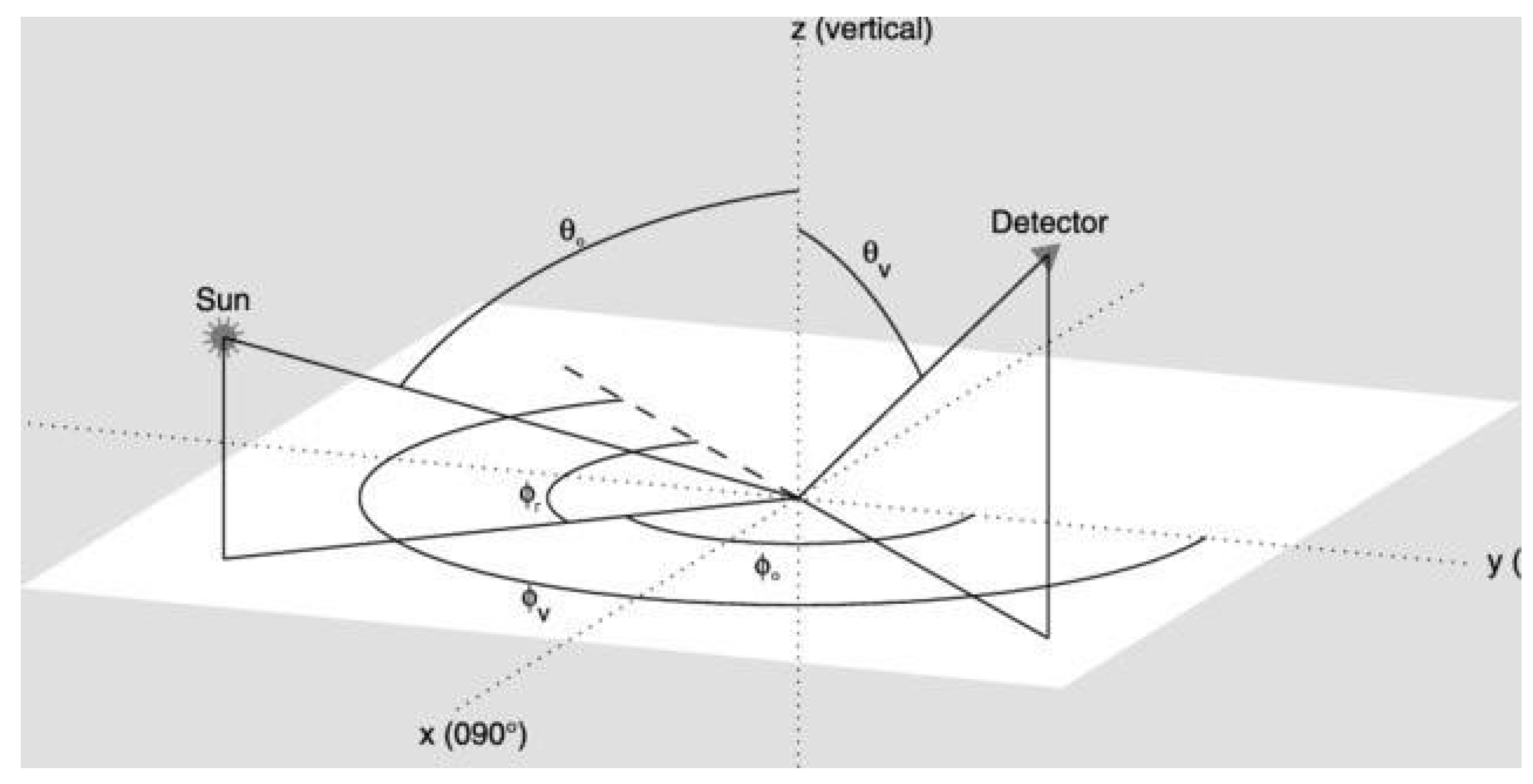
2.2.1. Geometry of the System

2.2.2. Reflectance, Spherical and Plane Albedo
2.2.3. Assumptions
2.2.4. Pre-Processing
2.2.5. Post Processing and Retrieval Quality Checks
2.3. Snow Property Retrieval
2.3.1. The Retrieval of Snow Grain Size and Albedo for Completely Snow-Covered Ground Scenes in Absence of Impurities
2.3.2. The Retrieval of Snow Impurity Properties
2.3.3. The Retrievals for Partially Snow-Covered Ground Scenes
2.3.4. Quality of Retrievals
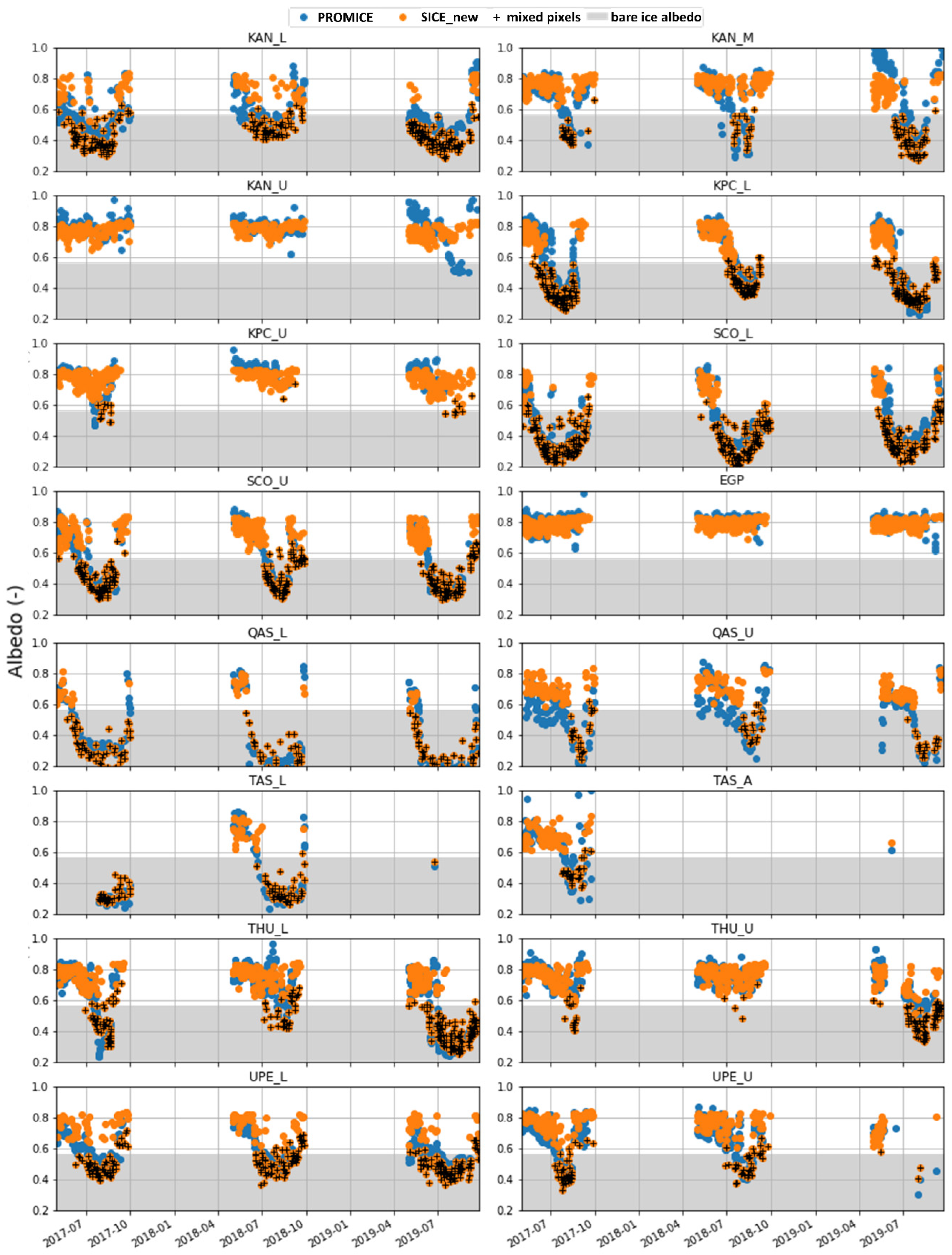
3. The Validation of the Algorithm
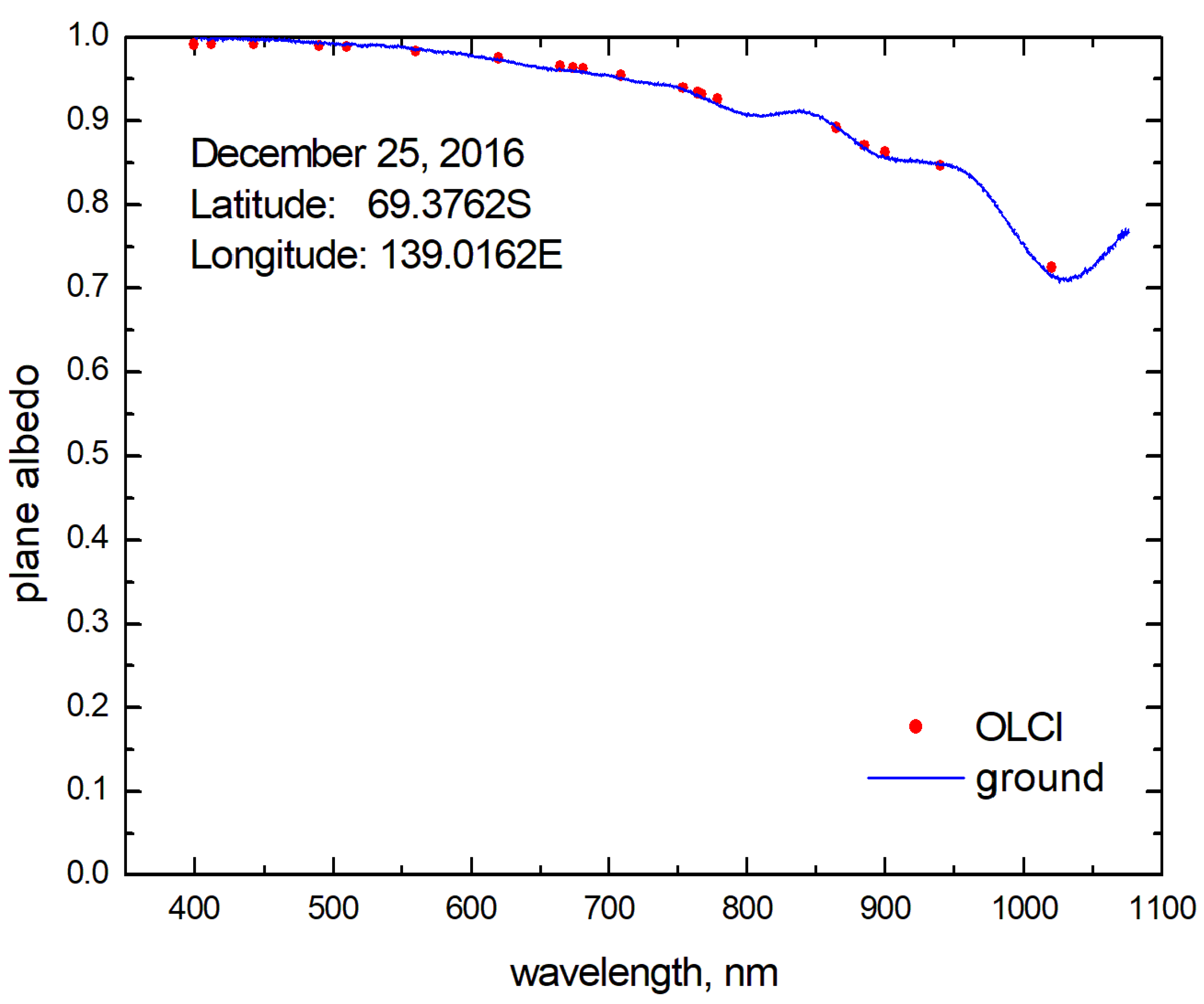
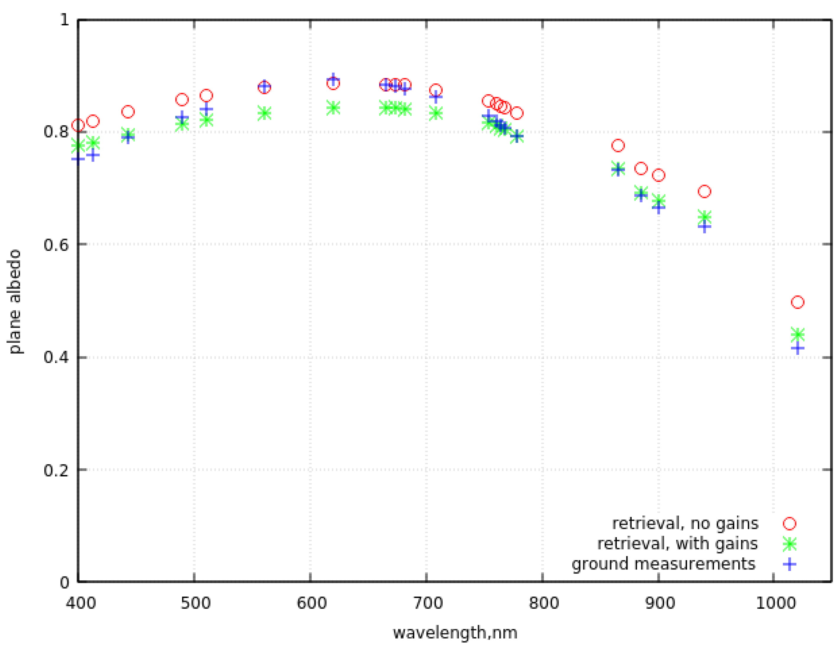
3.1. Spectral Albedo
3.2. Broadband Albedo
4. Examples of Retrievals
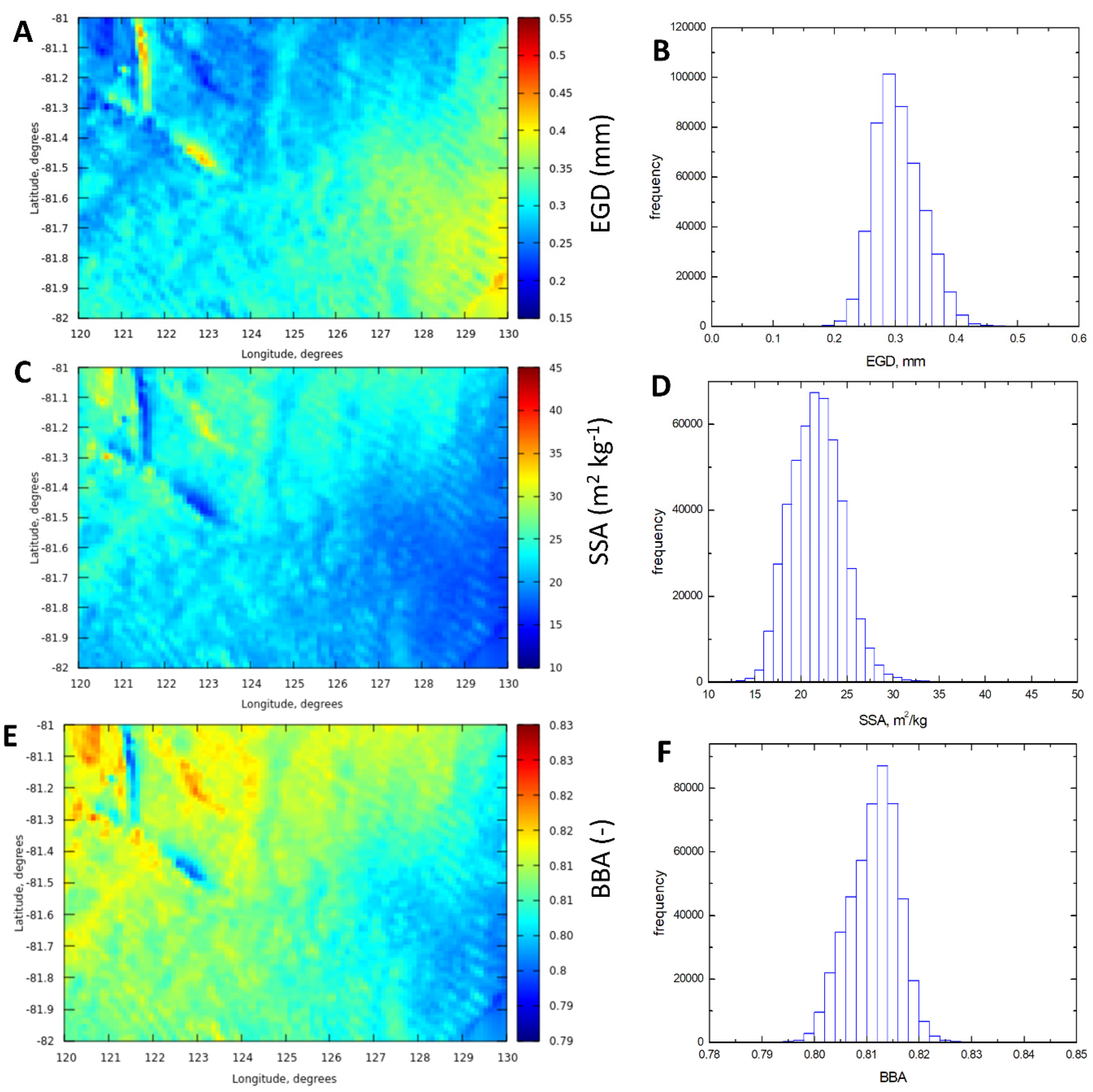
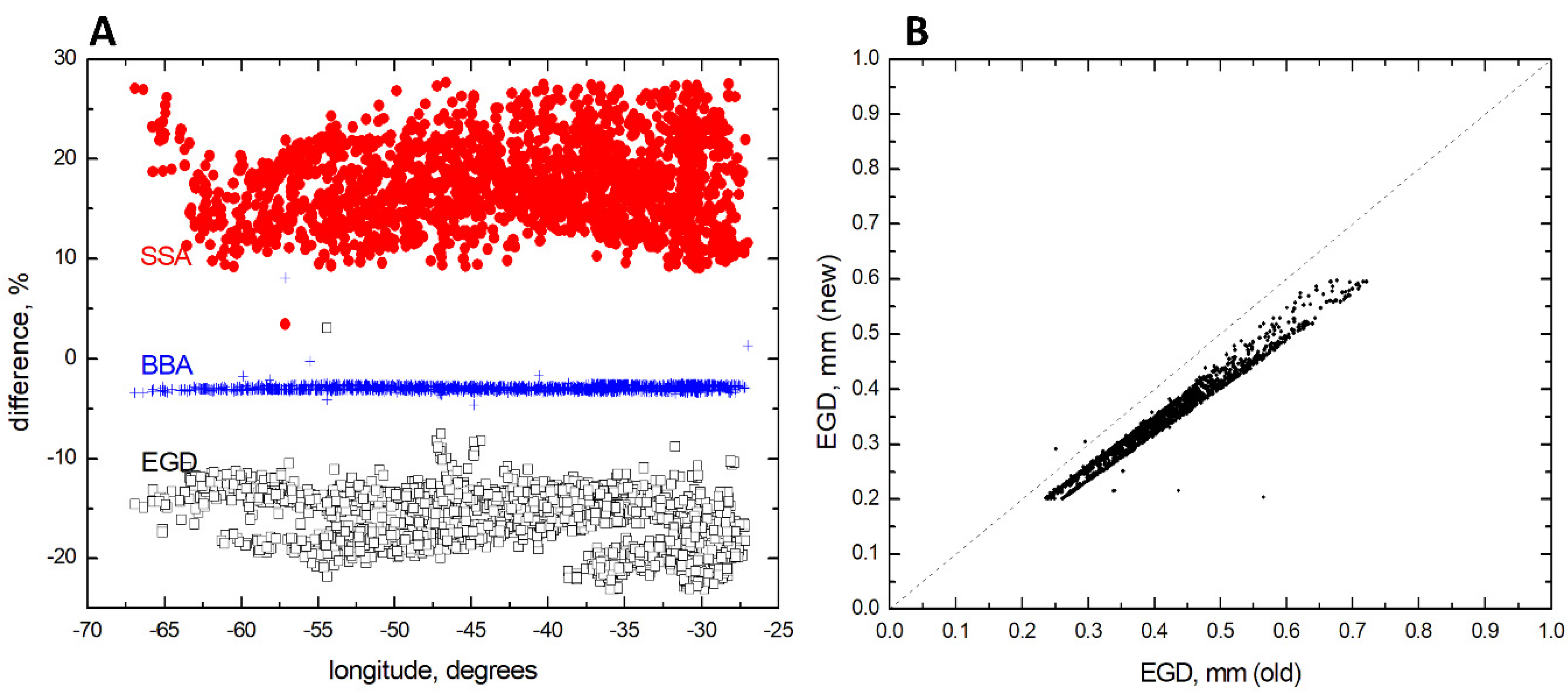
4.1. Antarctica
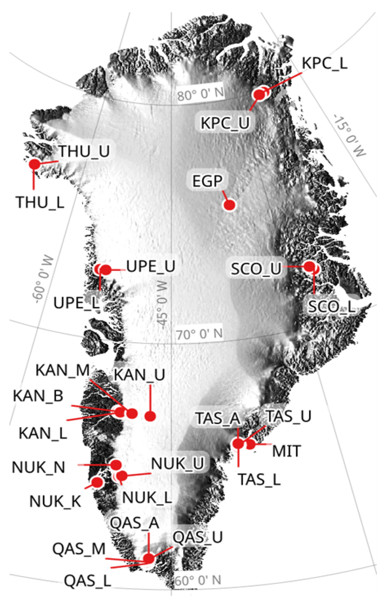
4.2. Greenland
5. Conclusions
Author Contributions
Funding
Data Availability Statement
Acknowledgments
Conflicts of Interest
Appendix A. OLCI Gains and Spectral Ice Refractive Index

| Wavelength, nm | OLCI Gain | Imaginary Part of Ice Refractive Index |
|---|---|---|
| 400 | 0.9755/0.9946/0.9597 | 6.27 × 10⁻¹⁰ |
| 412.5 | 0.9749/0.9901/0.9723 | 5.78 × 10⁻¹⁰ |
| 442.5 | 0.9689/0.9922/0.9716 | 6.49 × 10⁻¹⁰ |
| 490 | 0.9718/0.9862/0.9692 | 1.08 × 10⁻⁹ |
| 510 | 0.9757/0.9890/0.9764 | 1.46 × 10⁻⁹ |
| 560 | 0.9800/0.9911/0.9795 | 3.35 × 10⁻⁹ |
| 620 | 0.9783/0.9977/0.9771 | 8.58 × 10⁻⁹ |
| 665 | 0.9786/0.9968/0.9754 | 1.78 × 10⁻⁸ |
| 673.5 | 0.9791/0.9972/0.9734 | 1.95 × 10⁻⁸ |
| 681.25 | 0.9801/0.9980/0.9760 | 2.1 × 10⁻⁸ |
| 708.25 | 0.9855/1.0/1.0056 | 3.3 × 10⁻⁸ |
| 753.75 | 0.9855/1.0/0.9829 | 6.23 × 10⁻⁸ |
| 761.25 | 1.0/0.9968/1.0 | 7.1 × 10⁻⁸ |
| 764.375 | 1.0/0.9972/1.0 | 7.68 × 10⁻⁸ |
| 767.5 | 1.0/0.9980/1.0 | 8.13 × 10⁻⁸ |
| 778.75 | 0.9877/0.9978/0.9899 | 9.88 × 10⁻⁸ |
| 865 | 0.9860/1.0/1.0 | 2.4 × 10⁻⁷ |
| 885 | 0.9866/1.0/1.0182 | 3.64 × 10⁻⁷ |
| 900 | 1.0/1.0/1.0 | 4.2 × 10⁻⁷ |
| 940 | 1.0/1.0/1.0 | 5.53 × 10⁻⁷ |
| 1020 | 0.9132/0.9406/1.0 | 2.25 × 10⁻⁶ |
Appendix B. Generated Products
| Snow Product Name | Units | Snow Product Name | Units | ||
|---|---|---|---|---|---|
| 1 | Snow fraction | - | 16 | Mass absorption coefficient of dust particles at 660 nm | m2/g |
| 2 3 4 | Spectral spherical snow albedo Spectral planar snow albedo Spectral surface reflectance (for all OLCI channels) | - | 17 | Mass absorption coefficient of dust particles at 1000 nm | m2/g |
| 5 | Broadband snow albedo (plane and spherical, for three spectral ranges) | - | 18 | ECMWF total ozone column (TOC) given in OLCI files | DU |
| 6 | Snow specific surface area | m2 kg−1 | 19 | Retrieved TOC | DU |
| 7 | Snow grain diameter | mm | 20 | Normalized root-mean-square differences of registered and modelled TOA spectra using all OLCI channels | % |
| 8 | Concentration of pollutants (part per million weight) | ppmw (10−6) | 21 | The same as above except outside oxygen and water vapor absorption bands | % |
| 9 | Normalized difference snow index (NDSI) | - | 22 | Relative difference between OLCI and retrieved TOCs | % |
| 10 | Normalized difference bare ice index (NDBI) | - | 23 | Type of underlying surface (1—clean snow, 2—polluted snow, 3—partially snow covered) | - |
| 11 | Effective radius of dust grains | micron | 24 | Type of impurities (0—no impurities, 1—black carbon, 2—dust) | - |
| 12 | Effective absorption length | mm | 25 | Bare glacier ice index (1—glacier clean ice, 2—glacier polluted ice, 0—otherwise) | - |
| 13 | Reflectance of a nonabsorbing snow | - | 26 | Snow index (0—no snow, 1—snow) | - |
| 14 | Absorption Angström exponent of snow impurities | - | 27 | OLCI spectral index (OSI) | - |
| 15 | Impurity load parameter | 1/m |
References
- Hall, A. The role of surface albedo feedback in climate. J. Clim. 2004, 17, 1550–1568. [Google Scholar] [CrossRef]
- Vandecrux, B.; Box, J.E.; Wehrlé, A.; Kokhanovsky, A.A.; Picard, G.; Niwano, M.; Hörhold, M.; Faber, A.-K.; Steen-Larsen, H.C. The determination of the snow optical grain diameter and snowmelt area on the Greenland Ice Sheet using spaceborne optical observations. Remote Sens. 2022, 14, 932. [Google Scholar] [CrossRef]
- Skiles, S.M.; Flanner, M.; Cook, J.; Dumont, M.; Painter, T.H. Radiative forcing by light-absorbing particles in snow. Nat. Clim. Chang. 2018, 8, 964–971. [Google Scholar] [CrossRef]
- Warren, S.G. Can black carbon in snow be detected by remote sensing? J. Geophys. Res. Atmos. 2013, 118, 779–786. [Google Scholar] [CrossRef] [Green Version]
- Doherty, S.J.; Warren, S.G.; Grenfell, T.C.; Clarke, A.D.; Brandt, R.E. Light-absorbing impurities in Arctic snow. Atmos. Chem. Phys. Discuss. 2010, 10, 11647–11680. [Google Scholar] [CrossRef] [Green Version]
- Kokhanovsky, A.; Lamare, M.; Di Mauro, B.; Picard, G.; Arnaud, L.; Dumont, M.; Tuzet, F.; Brockmann, C.; Box, J.E. On the reflectance spectroscopy of snow. Cryosphere 2018, 12, 2371–2382. [Google Scholar] [CrossRef] [Green Version]
- Kokhanovsky, A.A.; Lamare, M.; Danne, O.; Brockmann, C.; Dumont, M.; Picard, G.; Arnaud, L.; Favier, V.; Jourdain, B.; Le Meur, E.; et al. Retrieval of Snow Properties from the Sentinel-3 Ocean and Land Colour Instrument. Remote Sens. 2019, 11, 2280. [Google Scholar] [CrossRef] [Green Version]
- Kokhanovsky, A.; Box, J.E.; Vandecrux, B.; Mankoff, K.D.; Lamare, M.; Smirnov, A.; Kern, M. The Determination of Snow Albedo from Satellite Measurements Using Fast Atmospheric Correction Technique. Remote Sens. 2020, 12, 234. [Google Scholar] [CrossRef] [Green Version]
- Wehrlé, A.; Box, J.E.; Niwano, M.; Anesio, A.M.; Fausto, R.S. Greenland bare-ice albedo from PROMICE automatic weather station measurements and Sentinel-3 satellite observations. GEUS Bull. 2021, 47. [Google Scholar] [CrossRef]
- Kokhanovsky, A. The Approximate Analytical Solution for the Top-of-Atmosphere Spectral Reflectance of Atmosphere—Underlying Snow System over Antarctica. Remote Sens. 2022, 14, 4778. [Google Scholar] [CrossRef]
- Kokhanovsky, A.A.; Lamare, M.; Rozanov, V. Retrieval of the total ozone over Antarctica using Sentinel-3 ocean and land colour instrument. J. Quant. Spectrosc. Radiat. Transf. 2020, 251, 107045. [Google Scholar] [CrossRef]
- Mazeran, C.; Ruescas, A. Ocean Colour System Vicarious Calibration Tool Documentation, EUMETSAT, EUM/19/SVCT/D2. 2020. Available online: https://www.eumetsat.int/media/47502 (accessed on 1 December 2022).
- Vandecrux, B.; Kokhanovsky, A.; Picard, G.; Box, J. pySICE: A python package for the retrieval of snow surface properties from Sentinel 3 OLCI reflectances (v2.1). Zenodo 2022. [Google Scholar] [CrossRef]
- Sobolev, V.V. Light Scattering in Planetary Atmospheres; Nauka: Moscow, Russia, 1975. [Google Scholar]
- Hudson, S.R.; Warren, S.G.; Brandt, R.E.; Grenfell, T.C.; Six, D. Spectral bidirectional reflectance of Antarctic snow: Measurements and parameterization. J. Geophys. Res. Earth Surf. 2006, 111. [Google Scholar] [CrossRef] [Green Version]
- He, C.; Flanner, M. Snow Albedo and Radiative Transfer: Theory, Modeling, and Parameterization; Springer Series in Light Scattering; Kokhanovsky, A., Ed.; Springer Nature: Cham, Switzerland, 2020; Volume 5, pp. 67–134. [Google Scholar]
- Qu, Y.; Liang, S.; Liu, Q.; He, T.; Liu, S.; Li, X. Mapping surface broadband albedo from satellite observations: A review of literatures on algorithms and products. Remote Sens. 2015, 7, 990–1020. [Google Scholar] [CrossRef] [Green Version]
- Aoki, T.; Kuchiki, K.; Niwano, M.; Kodama, Y.; Hosaka, M.; Tanaka, T.Y. Physically based snow albedo model for calculating broadband albedos and the solar heating profile in snowpack for general circulation models. J. Geophys. Res. Atmos. 2011, 116, D11114. [Google Scholar] [CrossRef]
- Metsämäki, S.; Pulliainen, J.; Salminen, M.; Luojus, K.; Wiesmann, A.; Solberg, R.; Böttcher, K.; Hiltunen, M.; Ripper, E. Introduction to GlobSnow Snow Extent products with considerations for accuracy assessment. Remote Sens. Environ. 2015, 156, 96–108. [Google Scholar] [CrossRef]
- Wehrlé, A.; Box, J.E. SICE Implementation of the Simple Cloud Detection Algorithm (SCDA) v2.0. 2021. Available online: https://dataverse.geus.dk/file.xhtml?persistentId=doi:10.22008/FK2/N0XWSJ/N2N2DT&version=1.0 (accessed on 1 December 2022). [CrossRef]
- Rozanov, V.V.; Rozanov, A.V.; Kokhanovsky, A.A.; Burrows, J.P. Radiative transfer through terrestrial atmosphere and ocean: Software package SCIATRAN. J. Quant. Spectrosc. Radiat. Transf. 2014, 133, 13–71. [Google Scholar] [CrossRef]
- Liou, K.N. An Introduction to Atmospheric Radiation; Academic Press: New York, NY, USA, 2002. [Google Scholar]
- Kokhanovsky, A.A. Snow Optics; Springer Nature: Cham, Switzerland, 2021. [Google Scholar]
- Kokhanovsky, A.A.; Zege, E.P. Scattering optics of snow. Appl. Opt. 2004, 43, 1589–1602. [Google Scholar] [CrossRef]
- Zege, E.P.; Ivanov, A.P.; Katsev, I.L. Image Transfer through Light Scattering Media; Springer: Berlin, Germany, 1991. [Google Scholar]
- Tomasi, C.; Petkov, B.H. Spectral calculations of Rayleigh-scattering optical depth at Arctic and Antarctic sites using a two-term algorithm. J. Geophys. Res. Atmos. 2015, 120, 9514–9538. [Google Scholar] [CrossRef]
- Six, D.; Fily, M.; Blarel, L.; Goloub, P. First aerosol optical thickness measurements at Dome C (East Antarctica), summer season 2003–2004. Atmos. Environ. 2005, 39, 5041–5050. [Google Scholar] [CrossRef]
- Warren, S.G.; Brandt, R.E. Optical constants of ice from the ultraviolet to the microwave: A revised compilation. J. Geophys. Res. Atmos. 2008, 113, D14220. [Google Scholar] [CrossRef]
- Kokhanovsky, A.A. Scaling constant and its determination from simultaneous measurements of light reflection and methane adsorption by snow samples. Opt. Lett. 2006, 31, 3282–3284. [Google Scholar] [CrossRef] [PubMed]
- Libois, Q.; Picard, G.; Dumont, M.; Arnaud, L.; Sergent, C.; Pougatch, E.; Sudul, M.; Vial, D. Experimental determination of the absorption enhancement parameter of snow. J. Glaciol. 2014, 60, 714–724. [Google Scholar] [CrossRef] [Green Version]
- Domine, F.; Taillandier, A.-S.; Simpson, W. A parameterization of the specific surface area of seasonal snow for field use and for models of snowpack evolution. J. Geophys. Res. Atmos. 2007, 112. [Google Scholar] [CrossRef]
- Libois, Q.; Picard, G.; Arnaud, L.; Dumont, M.; Lafaysse, M.; Morin, S.; Lefebvre, E. Summertime evolution of snow specific surface area close to the surface on the Antarctic Plateau. Cryosphere 2015, 9, 2383–2398. [Google Scholar] [CrossRef] [Green Version]
- Kokhanovsky, A.A. Broadband albedo of snow. Front. Environ. Sci. Inform. Remote Sens. 2021, 9, 757575. [Google Scholar] [CrossRef]
- Ångström, A. On the atmospheric transmission of Sun radiation and on dust in the air. Geogr. Ann. 1929, 11, 156–166. [Google Scholar]
- Hansen, J.E.; Travis, L.D. Light scattering in planetary atmospheres. Space Sci. Rev. 1974, 16, 527–610. [Google Scholar] [CrossRef]
- Iqbal, M. An Introduction to Solar Radiation; Elsiever: Amsterdam, The Netherlands, 1983. [Google Scholar]
- Kinne, S. Aerosol radiative effects with MACv2. Atmos. Meas. Tech. 2019, 19, 10919–10959. [Google Scholar] [CrossRef] [Green Version]
- Bond, T.; Bergstrom, R.W. Light Absorption by Carbonaceous Particles: An Investigative Review. Aerosol Sci. Technol. 2006, 40, 27–67. [Google Scholar] [CrossRef]
- Bond, T.C.; Doherty, S.J.; Fahey, D.W.; Forster, P.M.; Berntsen, T.; DeAngelo, B.J.; Flanner, M.G.; Ghan, S.; Kärcher, B.; Koch, D.; et al. Bounding the role of black carbon in the climate system: A scientific assessment. J. Geophys. Res. Atmos. 2013, 118, 5380–5552. [Google Scholar] [CrossRef]
- Caponi, L.; Formenti, P.; Massabó, D.; Di Biagio, C.; Cazaunau, M.; Pangui, E.; Chevaillier, S.; Landrot, G.; Andreae, M.O.; Kandler, K.; et al. Spectral- and size-resolved mass absorption efficiency of mineral dust aerosols in the shortwave spectrum: A simulation chamber study. Atmos. Chem. Phys. 2017, 17, 7175–7191. [Google Scholar] [CrossRef] [Green Version]
- Di Mauro, B.; Fava, F.; Ferrero, L.; Garzonio, R.; Baccolo, G.; Delmonte, B.; Colombo, R. Mineral dust impact on snow radiative properties in the European Alps combining ground, UAV, and satellite observations. J. Geophys. Res. Atmos. 2015, 120, 6080–6097. [Google Scholar] [CrossRef]
- Di Mauro, B.; Garzonio, R.; Rossini, M.; Filippa, G.; Pogliotti, P.; Galvagno, M.; di Cella, U.M.; Migliavacca, M.; Baccolo, G.; Clemenza, M.; et al. Saharan dust events in the European Alps: Role in snowmelt and geochemical characterization. Cryosphere 2019, 13, 1147–1165. [Google Scholar] [CrossRef] [Green Version]
- Di Mauro, B.; Garzonio, R.; Baccolo, G.; Gilardoni, S.; Rossini, M.; Colombo, R. Light-Absorbing Particles in Snow and Ice: A Brief Journey across Latitudes; Springer: Cham, Switzerland, 2021; pp. 1–29. [Google Scholar] [CrossRef]
- Dumont, M.; Arnaud, L.; Picard, G.; Libois, Q.; Lejeune, Y.; Nabat, P.; Voisin, D.; Morin, S. In situ continuous visible and near-infrared spectroscopy of an alpine snowpack. Cryosphere 2017, 11, 1091–1110. [Google Scholar] [CrossRef] [Green Version]
- Kokhanovsky, A.; Di Mauro, B.; Garzonio, R.; Colombo, R. Retrieval of dust properties from spectral snow reflectance measurements. Front. Environ. Sci. Inform. Remote Sens. 2021, 9, 644551. Available online: https://www.frontiersin.org/article/10.3389/fenvs.2021.644551 (accessed on 1 December 2022). [CrossRef]
- Kokhanovsky, A. Reflection of light from particulate media with irregularly shaped particles. J. Quant. Spectrosc. Radiat. Transf. 2005, 96, 1–10. [Google Scholar] [CrossRef]
- Picard, G.; Libois, Q.; Arnaud, L. Refinement of the ice absorption spectrum in the visible using radiance profile measurements in Antarctic snow. Cryosphere 2016, 10, 2655–2672. [Google Scholar] [CrossRef] [Green Version]
- Larue, F.; Picard, G.; Arnaud, L.; Ollivier, I.; Delcourt, C.; Lamare, M.; Tuzet, F.; Revuelto, J.; Dumont, M. Snow albedo sensitivity to macroscopic surface roughness using a new ray-tracing model. Cryosphere 2020, 14, 1651–1672. [Google Scholar] [CrossRef]
- Tuzet, F.; Dumont, M.; Arnaud, L.; Voisin, D.; Lamare, M.; Larue, F.; Revuelto, J.; Picard, G. Influence of light-absorbing particles on snow spectral irradiance profiles. Cryosphere 2019, 13, 2169–2187. [Google Scholar] [CrossRef] [Green Version]
- Denjean, C.; Formenti, P.; Desboeufs, K.; Chevaillier, S.; Triquet, S.; Maillé, M.; Cazaunau, M.; Laurent, B.; Mayol-Bracero, O.L.; Vallejo, P.; et al. Size distribution and optical properties of African mineral dust after intercontinental transport. J. Geophys. Res. Atmos. 2016, 121, 7117–7138. [Google Scholar] [CrossRef] [Green Version]
- Fausto, R.S.; van As, D.; Mankoff, K.D.; Vandecrux, B.; Citterio, M.; Ahlstrøm, A.P.; Andersen, S.B.; Colgan, W.; Karlsson, N.B.; Kjeldsen, K.K.; et al. Programme for Monitoring of the Greenland Ice Sheet (PROMICE) automatic weather station data. Earth Syst. Sci. Data 2021, 13, 3819–3845. [Google Scholar] [CrossRef]
- van As, D.; Fausto, R.S.; PROMICE Project Team. Programme for Monitoring of the Greenland Ice Sheet (PROMICE): First temperature and ablation records. GEUS Bull. 2011, 23, 73–76. [Google Scholar] [CrossRef] [Green Version]
- Broeke, M.V.D.; Reijmer, C.; Van De Wal, R. Surface radiation balance in Antarctica as measured with automatic weather stations. J. Geophys. Res. Atmos. 2004, 109. [Google Scholar] [CrossRef]
- Dickinson, R.E. Land surface processes and climate—Surface albedos and energy balance. Adv. Geophys. 1983, 25, 305–353. [Google Scholar]
- Henderson-Sellers, A.; Wilson, M.F. Surface albedo data for cliamtic modeling. Rev. Geophys. 1983, 21, 1743–1778. [Google Scholar] [CrossRef]
- Dickinson, R.E. Land processes in climate models. Remote Sens. Environ. 1995, 51, 27–38. [Google Scholar] [CrossRef]
- Peng, J.; Yu, Y.; Yu, P.; Liang, S. The VIIRS sea-ice albedo product generation and preliminary validation. Remote Sens. 2018, 10, 1826. [Google Scholar] [CrossRef] [Green Version]
- Gay, M.; Fily, M.; Genthon, C.; Frezzotti, M.; Oerter, H.; Winther, J.-G. Snow grain-size measurements in Antarctica. J. Glaciol. 2002, 48, 527–535. [Google Scholar] [CrossRef] [Green Version]
- Grenfell, T.C.; Warren, S.G.; Mullen, P.C. Reflection of solar radiation by the Antarctic snow surface at ultraviolet, visible, and near-infrared wavelengths. J. Geophys. Res. Earth Surf. 1994, 99, 18669–18684. [Google Scholar] [CrossRef]
- Pirazzini, R. Surface albedo measurements over Antarctic sites in summer. J. Geophys. Res. Earth Surf. 2004, 109. [Google Scholar] [CrossRef]
- Kuipers Munneke, P.; Reijmer, C.H.; Broeke, M.R.V.D.; König-Langlo, G.; Stammes, P.; Knap, W.H. Analysis of clear-sky Antarctic snow albedo using observations and radiative transfer modeling. J. Geophys. Res. Earth Surf. 2008. [Google Scholar] [CrossRef] [Green Version]
- Kuipers Munnike, P. Snow, Ice and Solar Radiation. Ph.D. Thesis, Institute for Marine and Atmospheric Research, Utrecht, The Netherlands, 2009. [Google Scholar]
- Kokhanovsky, A.; Gascoin, S.; Arnaud, L.; Picard, G. Retrieval of snow albedo and total ozone column from single-view MSI/S-2 spectral reflectance measurements over Antarctica. Remote Sens. 2021, 13, 4404. [Google Scholar] [CrossRef]
- Pernov, J.B.; Beddows, D.; Thomas, D.C.; Dall’osto, M.; Harrison, R.M.; Schmale, J.; Skov, H.; Massling, A. Increased aerosol concentrations in the High Arctic attributable to changing atmospheric transport patterns. NPJ Clim. Atmos. Sci. 2022, 5, 62. [Google Scholar] [CrossRef]


| Band | λ Centre (nm) | Width (nm) | Band | λ Centre (nm) | Width (nm) | Band | λ Centre (nm) | Width (nm) |
|---|---|---|---|---|---|---|---|---|
| 1 | 400 | 15 | 8 | 665 | 10 | 15 | 767.5 | 2.5 |
| 2 | 412.5 | 10 | 9 | 673.75 | 7.5 | 16 | 778.75 | 15 |
| 3 | 442.5 | 10 | 10 | 681.25 | 7.5 | 17 | 865 | 20 |
| 4 | 490 | 10 | 11 | 708.75 | 10 | 18 | 885 | 10 |
| 5 | 510 | 10 | 12 | 753.75 | 7.5 | 19 | 900 | 10 |
| 6 | 560 | 10 | 13 | 761.25 | 2.5 | 20 | 940 | 20 |
| 7 | 620 | 10 | 14 | 764.375 | 3.75 | 21 | 1020 | 40 |
| Parameter | Meaning | Equation |
|---|---|---|
| Cosine of viewing zenith angle | ||
| Cosine of solar zenith angle | ||
| Relative azimuthal angle | ||
| ( ) | The reflectance of snow at the idealized assumption that there is no light absorption in snow | |
| Anisotropy function | () | |
| The escape function | ||
| The normalized wavelength () | ||
| The impurity load parameter | ||
| m | The impurity absorption Angström parameter | |
| α | Bulk ice absorption coefficient | |
| The imaginary part of ice refractive index | ||
| L | The effective absorption length |
| Quantity | Symbol | Equation | Parameters |
|---|---|---|---|
| EGD | d | pL | p = 0.0625 |
| SSA | σ | q/L | q = 0.1047 m3/kg |
| Date | Location | m | γ, 1/mm | L, mm | d, mm | |||
|---|---|---|---|---|---|---|---|---|
| 17.04.2018 | Col du Lautaret (French Alps) | 3.04 (2.16) | () | 17.5 (23.9) | 9.61 (8.96) | 1.1 (1.5) | 82.6 (217.0) | 11.5 (18.1) |
| 17.05.2018 | Torgnon (Italian Alps) | 2.5 | 25.6 | 9.11 | 1.6 | 77.4 | 15.2 |
| Wavelength, nm | Dust MAC, 10−3 m2 g−1 | ||
|---|---|---|---|
| SICE without Gains | SICE with Gains | Denjean et al. [50] Caponi et al. [40] | |
| 428 | 47.7 | 21.1 | 37 |
| 532 | 24.6 | 13.2 | 20 |
| 660 | 12.8 | 8.3 | 11 * |
| 850 | 5.9 | 4.8 | 5 * |
| 1000 | 3.6 | 3.4 | 3 * |
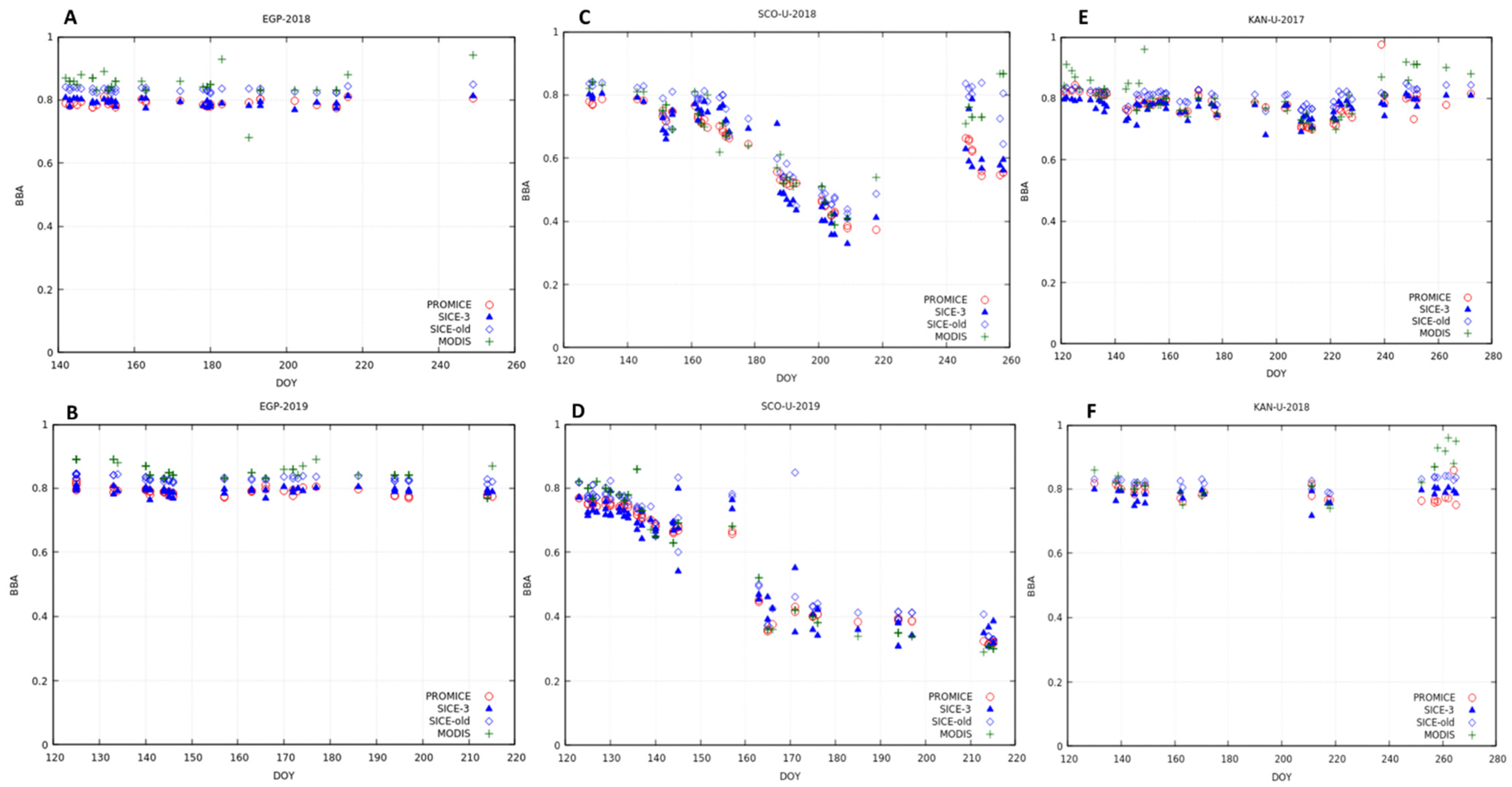
| Year | N | Yearly Average BBA | Yearly Average Relative Difference Relative to PROMICE (%) | Yearly Average Absolute Difference Relative to PROMICE (-) | |||||||
|---|---|---|---|---|---|---|---|---|---|---|---|
| PROMICE | SICE_New | SICE_Prev | MODIS | SICE_New | SICE_Prev | MODIS | SICE_New | SICE_Prev | MODIS | ||
| EGP | |||||||||||
| 2017 | 119 | 0.78 | 0.79 | 0.83 | 0.84 | 1.2 | 5.9 | 7.0 | 0.01 | 0.04 | 0.05 |
| 2018 | 35 | 0.79 | 0.79 | 0.83 | 0.85 | 0.1 | 5.4 | 7.5 | 0.00 | 0.04 | 0.06 |
| 2019 | 48 | 0.79 | 0.79 | 0.83 | 0.85 | −0.6 | 5.1 | 7.9 | 0.00 | 0.04 | 0.06 |
| SCO-U | |||||||||||
| 2017 | 88 | 0.51 | 0.53 | 0.58 | 0.54 | 2.8 | 13.7 | 5.3 | 0.02 | 0.07 | 0.03 |
| 2018 | 55 | 0.61 | 0.62 | 0.69 | 0.66 | 0.1 | 13.0 | 8.1 | 0.00 | 0.08 | 0.05 |
| 2019 | 69 | 0.60 | 0.60 | 0.64 | 0.62 | −0.6 | 6.7 | 1.3 | −0.01 | 0.04 | 0.02 |
| KAN-U | |||||||||||
| 2017 | 63 | 0.78 | 0.77 | 0.81 | 0.80 | −1.2 | 3.9 | 2.9 | 0.00 | 0.03 | 0.02 |
| 2018 | 25 | 0.79 | 0.78 | 0.82 | 0.83 | 0.0 | 4.7 | 5.8 | −0.01 | 0.04 | 0.04 |
| 2019 | 42 | 0.81 | 0.81 | 0.78 | 0.76 | −4.7 | −1.6 | −4.2 | −0.06 | −0.03 | −0.05 |
| Parameter | Average | Standard Deviation | Coefficient of Variance (%) | |||
|---|---|---|---|---|---|---|
| SICE_New | SICE_Prev | SICE_New | SICE_Prev | SICE_New | SICE_Prev | |
| EGD (mm) | 0.31 | 0.36 | 0.04 | 0.06 | 13.10 | 16.70 |
| SSA (m2 kg−1) | 21.75 | 18.78 | 2.82 | 4.10 | 13.00 | 21.80 |
| BBA (-) | 0.81 | 0.84 | 0.00 | 0.02 | 0.60 | 2.40 |
| Parameter | New Version | Old Version | Relative Difference, % |
|---|---|---|---|
| EGD, mm | 0.33 | 0.40 | −16.1 |
| SSA, | 20.95 | 17.55 | 17.5 |
| BBA | 0.79 | 0.81 | −2.9 |
Disclaimer/Publisher’s Note: The statements, opinions and data contained in all publications are solely those of the individual author(s) and contributor(s) and not of MDPI and/or the editor(s). MDPI and/or the editor(s) disclaim responsibility for any injury to people or property resulting from any ideas, methods, instructions or products referred to in the content. |
© 2022 by the authors. Licensee MDPI, Basel, Switzerland. This article is an open access article distributed under the terms and conditions of the Creative Commons Attribution (CC BY) license (https://creativecommons.org/licenses/by/4.0/).
Share and Cite
Kokhanovsky, A.; Vandecrux, B.; Wehrlé, A.; Danne, O.; Brockmann, C.; Box, J.E. An Improved Retrieval of Snow and Ice Properties Using Spaceborne OLCI/S-3 Spectral Reflectance Measurements: Updated Atmospheric Correction and Snow Impurity Load Estimation. Remote Sens. 2023, 15, 77. https://doi.org/10.3390/rs15010077
Kokhanovsky A, Vandecrux B, Wehrlé A, Danne O, Brockmann C, Box JE. An Improved Retrieval of Snow and Ice Properties Using Spaceborne OLCI/S-3 Spectral Reflectance Measurements: Updated Atmospheric Correction and Snow Impurity Load Estimation. Remote Sensing. 2023; 15(1):77. https://doi.org/10.3390/rs15010077
Chicago/Turabian StyleKokhanovsky, Alexander, Baptiste Vandecrux, Adrien Wehrlé, Olaf Danne, Carsten Brockmann, and Jason E. Box. 2023. "An Improved Retrieval of Snow and Ice Properties Using Spaceborne OLCI/S-3 Spectral Reflectance Measurements: Updated Atmospheric Correction and Snow Impurity Load Estimation" Remote Sensing 15, no. 1: 77. https://doi.org/10.3390/rs15010077