Article

A Multi-Scale Feasibility Study into Acid Mine Drainage (AMD) Monitoring Using Same-Day Observations

1
Environment and Sustainability Institute, University of Exeter, Penryn Campus, Penryn TR10 9FE, UK
2
Camborne School of Mines, University of Exeter, Penryn Campus, Penryn TR10 9EZ, UK
3
Carrack Consulting, Laburnum House, Vogue, St Day, Redruth TR16 5NH, UK
4
North Coast Consulting, Unit 2, Mount Pleasant Ecological Park, Chapel Hill, Porthtowan TR4 8HL, UK
*
Author to whom correspondence should be addressed.
Remote Sens. 2023, 15(1), 76; https://doi.org/10.3390/rs15010076
Submission received: 10 November 2022 / Revised: 14 December 2022 / Accepted: 21 December 2022 / Published: 23 December 2022
(This article belongs to the Special Issue Remote Sensing Solutions for Mapping Mining Environments)

Abstract

:
Globally, many mines emit acid mine drainage (AMD) during and after their operational life cycle. AMD can affect large and often inaccessible areas. This leads to expensive monitoring via conventional ground-based sampling. Recent advances in remote sensing which are both non-intrusive and less time-consuming hold the potential to unlock a new paradigm of automated AMD analysis. Herein, we test the feasibility of remote sensing as a standalone tool to map AMD at various spatial resolutions and altitudes in water-impacted mining environments. This was achieved through the same-day collection of satellite-based simulated Sentinel-2 (S2) and PlanetScope (PS2.SD) imagery and drone-based UAV Nano-Hyperspec (UAV) imagery, in tandem with ground-based visible and short-wave infrared analysis. The study site was a historic tin and copper mine in Cornwall, UK. The ground-based data collection took place on the 30 July 2020. Ferric (Fe(III) iron) band ratio (665/560 nm wavelength) was used as an AMD proxy to map AMD pixel distribution. The relationship between remote-sensed Fe(III) iron reflectance values and ground-based Fe(III) iron reflectance values deteriorated as sensor spatial resolution decreased from high-resolution UAV imagery (<50 mm2 per pixel; r2 = 0.78) to medium-resolution PlanetScope Dove-R (3 m2 per pixel; r2 = 0.51) and low-resolution simulated Sentinel-2 (10 m2 per pixel; r2 = 0.23). A fractioned water pixel (FWP) analysis was used to identify mixed pixels between land and the nearby waterbody, which lowered spectral reflectance. Increases in total mixed pixels were observed as the spatial resolution of sensors decreased (UAV: 2.4%, PS: 3.7%, S2: 8.5%). This study demonstrates that remote sensing is a non-intrusive AMD surveying tool with varying degrees of effectiveness relative to sensor spatial resolution. This was achieved by identifying and successfully mapping a cross-sensor Fe(III) iron band ratio whilst recognizing water bodies as reflectance inhibitors for passive sensors.

Graphical Abstract

1. Introduction

Acid mine drainage (AMD) is the product of a series of reactions involving the oxidation of sulphide-bearing minerals, such as pyrite (FeS2), pyrrhotite (FeS), and arsenopyrite (FeAsS), with oxygen, water, and bacteria [1]. These reactions result in the release of protons, sulphate, and metal(loids) to waters, and ultimately, produce low pH and metal(oid)-rich sulfuric acid (AMD), which can severely contaminate receiving surface and groundwaters, soils and sediments [1,2,3,4]. Acid drainage may form naturally (acid rock drainage) [5] or by mining (acid mine drainage), with a continual need to monitor both. Above-ground mines cover more than 57 thousand km2 globally [6]. The costs of detecting AMD at mine sites using traditional methods, with a view to remediating or managing it, are significant, and thus, can be a substantial burden upon taxpayers and mining companies [7]. The scale of the problem is truly colossal: total worldwide liability associated with the current and future remediation of AMD is of the order of USD 100 B [8].
The breakdown of the Fe-bearing sulphides generates Fe2+, which is oxidized and used by chemotrophic microorganisms for energy generation. This, in turn, produces even more sulfuric acid through the production of Fe3+, which can act as an oxidant of the sulphides [2,3]. The solubility of Fe3+ at near-neutral pH is low, and thus, Fe(III) iron oxyhydroxide solids form rapidly. Fe(III) iron oxyhydroxides can be regarded as proxies for AMD because they are formed from it. They are also characterised by high concentrations of potentially toxic metal(loids) that they incorporate from the AMD. Fe2+ alteration can create a suite of secondary minerals (oxides, sulfates, carbonates, and more), such as goethite, hematite, and jarosite, which often exhibit similar colours [9]. pH plays a crucial role of secondary mineral precipitation and control, where goethite forms between pH 2 and12, and hematite at pH 7–9 [9,10,11]. Jarosite forms a magnitude lower in comparison (pH 1–3) [12]. As a known set of secondary mineral products exhibit an orange to red colour (with high concentrations of Fe (III)), they are distinguishable via remote sensing methods and have previously been used as proxies of AMD and iron ore deposits [13,14,15,16]. Band ratio operations are a well-established method that has been used as an effective geological surveying tool for decades, targeting and isolating geological material through their unique spectral signatures [17]. It is both low in cost as well as computational demand and covers vast areas in a short timeframe.
Remote sensing and band operations are useful tools, but band ratio products do not guarantee mineral presence with absolute certainty due to environmental interference [18]. Therefore, ground truthing is crucial and, in combination with the remote-based surveillance of AMD-impacted landscapes, has been successfully used to help identify mine waste by using band ratios for specific iron absorption features [15]. Ref. [19] successfully used ground-based reflectance spectroscopy to identify a suite of secondary iron oxide minerals indicative of the subaerial oxidation of pyrite. Multiple satellites can be used to increase the accuracy of AMD detection in mining environments by using a multi-sensor process chain alongside ground verification. A prerequisite is identifying a series of instruments with spectral sensitivities that overlap and cover Fe(III) iron signatures (Table 1). Using an interoperable set of wavelength bands is an effective method to link multispectral and hyperspectral observations using ground-based spectroscopy [16].
Environments containing AMD are prone to morphological change. It is, therefore, important that the capture of spectra is carried out in the shortest time window possible, preferably on the same day. This has not previously been attempted. Testing the feasibility of multiple spectral devices within real-world conditions is important to determine how spatial resolution impacts the ability to detect AMD. Furthermore, it is important to explore each sensor’s resilience toward mixed pixels caused by nearby water bodies (often associated with AMD deposits). Sudden changes in soil moisture can lead to an overall reduction in soil reflectance for all wavelengths, as when soil moisture levels increase, reflection decreases for most soil types [25]. The use of binary water masking is often the go-to method to deal with water in mining environments, which is an indiscriminative method. This study aims to fill this research gap by observing the impacts that spatial resolution and waterbodies have on the detection and delineation of surface AMD deposits at a representative AMD site in Cornwall, UK, through the same-day data capture of ground-, air-, and space-borne spectroscopy.

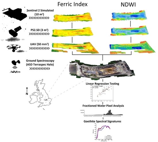
2. Materials and Methods

2.1. Study Area

Wheal Maid (50°14′14.3196″N 5°9′40.7232″W, see Figure 1) is typical of AMD-affected sites globally and it is located within the Cornish Mining UNESCO site. Wheal Maid is a good candidate for a same-day remote sensing case study with its contrasting and distinctive mine waste colours [26], and its lack of vegetation that passive sensors cannot penetrate. Wheal Maid’s mine waste has been subject to much ground-based research [26,27,28,29,30] but had yet to be the subject of a remote sensing-based multi-scale study prior to this work.
Wheal Maid consists of two tailing lagoons, with the lower lagoon found at the centre (Figure 1). The valley of Wheal Maid was used as an infill tailings repository spanning approximately 0.08 km2 and containing around 220,000 m3 of fine-grained tailings material discharged from Mount Wellington Mine between 1976 and 1981 [31,32]. The lower lagoon contains grey tailings with visible pyrite crystals and fine-grained red, brown, and yellow marbled tailings that remain un-vegetated [19,27].

2.2. Sampling Plans and Geospatial Error

The sampling campaign occurred on 30 July 2020. It involved the use of a high-precision Global Navigation Satellite System (Trimble R10) position device to determine the coordinates of samples along an unbiased 10 m × 10 m grid (as displayed in Figure 1). Twice the distance root mean square (2DRMS-2D) was calculated for the ground-based spectrometer (see Equation (1)). This helped to account for geospatial error and align satellite images to allow for statistical comparison. For the GNSS Trimble R10, a standard deviation of a geodetic latitude and longitude of 50 mm2 was reported, and HeadWall Photonics Incorporated [22] reported a 1 m2 circular error probability (CEP). This was converted into 2DRMS by multiplying it with the conversion value of 2.4022 [33]. The 2DRMS equation used was as follows:
2 D R M S = 2 × ( σ x ) 2 + ( σ y ) 2
Here, σ x represents the standard deviation of geodetic latitude, and σ y represents the standard deviation of geodetic longitude. After the 2DRMS was calculated, sample locations were plotted in ArcGIS Pro (3.0.2) [34] and converted into circular polygon features. This enabled the extraction of reflectance data overlapping with Wheal Maid’s central water body. We tested the Halo handheld spectrometer’s on-board GPS, which produced a circle feature with an 18.13 m2 area. The GNSS Trimble R10 produced circles with a 0.062 m2 area.

2.3. Data Acquisition

2.3.1. ASD TerraSpec Halo Handheld Spectrometer Mineral Identifier

The TerraSpec Halo handheld spectrometer Mineral Identifier [21] is a portable near-infrared spectrometer with a visible near-infrared (VNIR: 350–1000 nm) and near-infrared (SWIR: 1001–2500 nm) range [20]. It has an onboard GPS with a circular error probability of 1 m2 [35]. The Halo handheld spectrometer captures spectral, mineral, and scalar results. Scalar values provide information on the sample’s crystallinity and/or composition, which can serve as supplementary vectors to potential mineralization [20]. The Halo handheld spectrometer is able to capture Fe(III) iron mineral intensity as a scalar. This scalar depends on Fe(III) iron mineral surface abundance, and operates by calculating the ratio of the reflectance values found at a 742 nm to 500 nm wavelength. The higher the Fe3+i value recorded by the Halo handheld spectrometer, the more intense the Fe3+ absorption. The Halo handheld spectrometer was used to help with ground-to-air and space linear regression and correlation testing.
The Halo handheld spectrometer was deployed on 30 July 2020, taking samples at a 10 × 10 m grid along the Wheal Maid valley. The Halo handheld spectrometer’s window was wiped with a lint-free, nonabrasive cloth. Calibration was performed using the white reference disk provided. Fe3+i values were exported via the Halo handheld spectrometer Manager as ASD binary and ASCII files for the Fe(III) iron pixel distribution maps.

2.3.2. UAV Nano-Hyperspec

Texo DSI [36] and HeadWall Photonics Incorporated provided a Nano-Hyperspec visible near-infrared (VNIR) Imaging Sensor on a six-rotor UAV [37]. This sensor had 12-bit depth imagery, a spatial resolution of ≈50 mm2, and pixel dispersion at 2.2 nm/pixel (270 bands over 400–1000 nm). It was operated by a Texo unmanned aircraft system (UAS) pilot as a ground-based controller on 30 July 2020, at noon GMT over Wheal Maid. The flight path was pre-programmed to improve resolution and drone orientation. The GNSS Trimble R10 provided position data via ground control points (GCPs) for image ortho-rectification and stitching. Points that were >50 degrees in slope gradient were omitted from the sampling plan, as this exceeded the Nano-Hyperspec sensors. Eight data strips were collected. Due to the high precision of the UAV raster image using multiple GCPs, the UAV orthoreferenced Nano-Hyperspec image acted as the master image for co-registration of the remaining instrument images. All other instruments’ images had varying georeferencing procedures during their post-processing, so to align all instruments, a common GCP system with the highest precision, to which all other images were corrected to, was used. A geo-referenced digital terrain model (DEM) of Wheal Maid Valley was created through overlapping aerial photographs in Geographic Tagged File Format (GeoTIFFs) [38]. This was delivered as a 2 GB, 11 mm2 ground sample distance (GSD) TIFF file.
Fe(III) iron band ratio surface reflectance images were provided by HeadWall Photonics and Texo DSI after their post-processing procedures were conducted. The 2DRMS polygons were intersected with the Normalized Difference Water Index (NDWI) and Fe(III) iron rasters after the data strips had been mosaiced. UAV strips south of the central lower lagoon were missing or encompassed dead pixels due to the corrupted strip.

2.3.3. PlanetScope Dove-R

The sensor onboard the PlanetScope Dove satellite constellation is named PS2, which is paired with a 2D frame detector; the detector has 6600 pixels across by 4400 lines down with 4 channels (blue, green, red, and NIR). PS2.SD bands are interoperable with those of Sentinel-2. This allowed for the creation of a simulated Sentinel-2 image. PlanetScope Dove-R 3 m2 per pixel resolution surface reflectance images were exported using the Planet Explorer interface [39] and imported to ArcGIS for post-processing. PlanetScope (PS2.SD) analytic assets are multispectral imagery that come orthorectified, calibrated, and corrected for sensor artifacts and atmospheric interference. PlanetScope PS2.SD was able to capture clear surface reflectance images of the site, which provided the opportunity for Sentinel-2 simulation due to the spectral range similarities of both sensors, which have previously been used to improve each other’s remote sensing applications [40]. Final images (including a top of atmosphere (TOA) reflectance version for the fractioned water pixel (FWP) analysis) were exported for the post-processing steps. Surface reflectance images were used for correlation testing.
For the FWP analysis and Otsu thresholding, additional steps were taken for the TOA image, which included masking cloud interferences’ cloud shadow, haze, and corrupted pixels using the useable data mask (UDM2 metadata file as per [41,42]. TOA image PS2.SD images come in 16-bit with values as watts per steradian per square meter (W/m2 sr µm), and these were converted to reflectance using the reflectance coefficients provided in the metadata files. The UDM2 labelled each image pixel using a convolutional neural network [43].
The PS2.SD image taken on 30 July 2020 was used to create a simulated surface reflectance Sentinel-2 image by matching the Sentinel-2 sensor’s spectral and spatial resolution, as the Sentinel-2 image was missing due to cloud cover during satellite pass over. This was achieved by increasing the raster cell size to that of Sentinel-2 (10 × 10 m2) using a resampling tool and shifting cells to the UAV master image via co-registration. The simulated Sentinel-2 RGB image and Fe(III) iron distribution map closely resembled a Sentinel 2 image and map taken on 7 August 2020. The simulated image underwent the same post-processing treatment as the PS2.SD images.
In total, six suitable images were identified. The products were 32-bit floating-point single band images exported for post-processing via the Planet Explorer interface.

2.3.4. Sentinel-2 2A

Sentinel 2 2A imagery was exported using Google Earth Engine (GEE) [44] API. A geometry polygon was first constructed as an area of interest around Wheal Maid tailing repository encompassing the central lower lagoon and used a date filter between 1 July 2018 and 1 August 2018. For JavaScript code, see ‘Data Availability Statement’.

2.4. Spectral Data Post-Processing

2.4.1. Unsupervised Band Ratio Classification of Fe(III) Iron and Pixel Distribution Maps

Previous studies have positively identified the absorption feature for endmembers such as Fe(III) iron, with wavelengths at 400–900 nm, and identified satellites (ASTER, LANDSAT, Sentinel-2) with bands that are operational within this region of the electromagnetic spectrum [17,18,45]. The ASD Halo handheld spectrometer Fe3+i scalar feature covers 500 nm to 742 nm; UAV Texo Nano-Hyperspec bands cover 665 nm and 560 nm; PS2.SD (multispectral imaging) MSI has bands 2 and 3, 566 nm and 666 nm, respectively; Sentinel-2 MSI bands 4 and 3 cover 560 nm to 665 nm. These interoperable bands were used in band combinations to create Fe(III) abundance maps using band parameter combinations and methodologies as set out by [14,17,46]; for example, dividing the red and green band to cover both spectral peaks in Fe3+ in the red spectrum, and absorption in the green spectrum. Past research also shows that the spectral pattern of secondary iron oxides shows strong absorption in the blue, green, and NIR bands, and strong reflection in the red bands [17,47,48,49]. For PS2.SD, this was achieved by dividing bands 3/bands 2 (for Fe3+), performed through the use of ArcGIS raster functions.
Extracted Fe(III) iron values from the band ratio combination maps for all instruments were imported as CSV databases into IBM SPSS Statistics 27, alongside the Halo handheld spectrometer results collected on 30 July. Datasets that were not normally distributed (such as the Halo handheld spectrometer Fe3+i dataset) underwent Box–Cox power transformation to identify the corresponding Lambda values. Reciprocal power transformations were recommended and performed. The normality of the transformed data was confirmed by checking for normal distribution via plotting probability plots and histograms in SPSS and performing a Kolmogorov–Smirnov test [50] for normality. All Fe(III) iron reflectance scatterplots were fitted with linear regression models to test how well air- and space-borne observations predict Halo handheld spectrometer ground-based observations. To test the strength of the relationship between aerial and ground Fe (III) iron spectral reflectance, both the correlation coefficients and coefficient of determinations were calculated. These permitted testing of the hypothesis that, as the air- and space-borne Fe(III) iron reflectance values increase, so do the aerial Fe(III) iron reflectance values. When datasets were flagged for containing extreme outliers during the regression analysis due to saturated or defective pixels, a bivariate outlier analysis was performed to help identify them for further scrutiny.

2.4.2. NDVI, NDWI, and Fractioned Water Pixel Analysis

To identify and mask water and vegetation in the remote sensing data sets, the Normalized Difference Vegetation Index (NDVI) [51] and Normalized Difference Water Index (NDWI) [52] were calculated using the equations below:
NDVI = (Red − NIR)/(NIR + Red)
NDWI = (Green − NIR)/(NIR + Green)
The NDVI ranges from −1 to +1, where values closer to 1 indicate increased green leaf density, and closer to −1 equate to clear water, whereas barren rock exhibits very low NDVI. The NDWI also ranges from −1 to +1, where values closer to 1 usually correspond to water bodies, and between 0 and 0.5 (depending on the instrument and ground conditions) is either land or urbanized areas.
Due to the close proximity between AMD and the water deposits, this study adapted a water classification methodology that was previously used in [41,42], using atmospheric screened TOA images to identify regions of mixed pixels (that interfere with Fe(III) iron classification). The use of band ratios with TOA-R images has the advantage of feasibly yielding indices that are atmospherically stable enough for delineation purposes [11]. However, the use of TOA images should be restricted to simplistic classifications [42]. The equations can be found below:
LL = heightlp − 0.9 ×promlp
WL = heightwp − 0.9 ×promwp
where LL and WL stand for land limit and water limit, respectively. Both LL and WL were used as 100% land and water thresholds. heightlp and heightwp are maximum heights of the land and water peaks, whereas promlp and promwp are the respective prominence (maximum point of elevation versus its depth) of the land and water peaks. FWPtotal is the total percent of mixed water pixels as calculated for the PS2.SD, Sentinel-2 (simulated), and UAV images taken on the 30 July 2020..
In order to generate the NDWI histograms needed for the above FWP analysis, a modified OTSU adaptive thresholding [53] methodology was used to create buffered polygon features needed to capture the maximum extent of the waterbody at Wheal Maid and some of the surrounding land and vegetation. Buffered water polygons around Wheal Maid’s central lower lagoon were intersected with the NDWI images, and the values were extracted so that histograms could be made for the FWP analysis.
An NDWI pixel distribution graph was generated for each instrument, which needed to exhibit sufficient bi-model distribution that could be divided into two distinct peaks (one peak for water, the other for land). The plateau between both land and water peaks was then used to identify the region of mixed pixels, which can impact Fe(III) iron values.

2.4.3. Spectral Signatures of Known Fe(III) Iron Occurrences

Best practice and design were followed to create spectral signature graphs for all air and spaceborne sensors [54]. Using the results of the ground spectroscopy sampling campaign, an area with known Fe (III) secondary mineral occurrences (specifically goethite) was selected to host four training sites, which in this case were the north embankment of the lower lagoon, home to Wheal Maid’s marbled tailings [25]. The spectral signature data recognized as goethite by the Halo handheld spectrometer device were exported and imported in R [55] as an ASD binary file, where the meta and reflectance data were extracted and displayed as spectral signature response curve diagrams of the four Halo handheld spectrometer goethite samples. These were cross-referenced with a known goethite spectral response curve [13]. This acted as a baseline to compare with the spectral output of the devices used in this study. Areas of interest were drawn across four training sites using ArcGIS, and the spectral information of all available bands across Sentinel-2 2A, PS2.SD, and UAV Nano-Hyperspec sensors were extracted (using bottom-of-atmosphere surface reflectance images from July 2020). The spectral signatures across all sensors were imported into GraphPad PRISM (9.4.1) [56] and displayed as mean line graphs.

3. Results

3.1. Fe(III) Iron Distribution Maps and Spectral Linear Regression

A simple linear regression model was used to test if Fe(III) iron spectral values derived from aerial and spaceborne imagery significantly predicted the ground-based Fe(III) iron spectral values at Wheal Maid. The results of the main regression test between the Fe(III) iron values taken by the highest spatial resolution (< 50 mm2) sensor onboard UAV and ground-based Fe(III) iron reflectance values revealed that the model could explain 77.6% of the total variance (Figure 2c). The overall regression was statistically significant (R2 = 0.776, F(1, 32) = 110.67, p < 0.000), and the Fe(III) iron reflectance values from the Nano-Hyperspec sensor onboard the UAV significantly predicted the ground-based Fe(III) iron reflectance values (β1 = 0.998, p < 0.000). When the spatial resolution of the sensors began to decrease (inversely, pixel size began to increase), the explanatory variables’ (air- and space-borne Fe(III) iron values) ability to predict the response variable (ground-based Fe(III) iron values) diminished, albeit remaining statistically significant across all sensors (low and moderate correlation for Sentinel-2 and PlanetScope PS2.SD, respectively). The remainder of the regression model results between PS.2SD, S.2 (simulated), and the ground readings can be found in Figure 2a–c.
The layered raster models’ scenes depicting Fe(III) iron pixel distribution maps in Figure 2a–c) demonstrate that Fe(III) iron is concentrated around the perimeter of the central lower lagoon. The central lower lagoon is clearly visible in Figure 2e’s natural image of Wheal Maid (taken on 30 July 2020), as is the grey and marbled tailing distribution. The tiered raster models begin with the lowest resolution instrument, labelled (a) Sentinel-2 (simulated), and progress to the medial resolution (b) PlanetScope 2.SD, up to the highest resolution of c) UAV Nano-Hyperspec. The western part of Wheal Maid’s lower lagoon (grey tailings area) remained largely uninfluenced by surface Fe(III) iron in these maps, and the area remains largely yellow to green (Figure 2c). Fe(III) iron designated pixels were predominantly located below Wheal Maid’s winter water level. The Halo handheld spectrometer’s Kriging model in Figure 2d shows interpolation between Fe3+i point data taken across Wheal Maid, where an easterly retreat in the winter water level can be seen; the largest reflection occurred on marbled tailings.
The regression model with the highest ability to predict ground values was recorded between the high-resolution UAV Nano-Hyperspec sensor and Halo handheld spectrometer ground reflectance values. Corresponding regression scatterplots can be found below the tiered raster model scenes (Figure 2f–h). Increased homoscedasticity can be seen within the residuals when progressing from Figure 2f (simulated Sentinel-2) to Figure 2h (UAV Nano-Hyperspec).

3.2. NDWI and FWP Analysis Results

The NDWI band ratio indices calculated for all RGB images are compiled in Figure 3. The Wheal Maid DEM is included as the base layer. NDWI index value ranges differed amongst the instruments due to radiometric nuances in the spectral bands (as seen in Figure 3). The FWP analysis helped to identify maximum water and land limits, and these were plotted as histograms (Figure 3e–g). These charts descend in order of increasing spatial resolution, moving from multispectral to hyperspectral sensors. Each of the sensor’s NDWI rasters is accompanied by its corresponding FWPtotal from a–c, starting with Sentinel-2 (simulated) (a) and ending with the UAV raster (c). FWPtotal exhibits an inverse relationship, as FWPtotal increased as the instrument’s spatial resolution decreased. The simulated Sentinel-2 image had an FWPtotal of 8.5%; PlanetScope FWPtotal: 3.7%; and UAV Nano-Hyperspec FWPtotal: 2.4%.
NDWI histograms (Figure 3e–g) exhibited weakly bimodal distributions with land peaks being more prominent due to greater pixel count, as nearby water bodies were relatively small. The identified water and land limits differed amongst the instruments. The Sentinel-2 (simulated) and PlanetScope FWP plateau ranged from 0.17 to 0.25 and from 0.16 to 0.19, respectively, whereas UAV Nano-Hyperspec exhibited a more commonly reported NDWI range of 0.5 to 0.75, where the water limit maximum was closer to 1. The histograms exhibited a weak multimodal distribution, where a third lesser peak would arise left of the land peak.

4. Discussion

4.1. Remote Sensing as Means of Detecting AMD

The results show that all sensors were able to detect AMD and delineate it independently or in a multi-sensor configuration. However, UAV had the highest success. Recent attempts in AMD monitoring have seen similar success, with similar correlation rates between UAV and ground-based readings (R2 ≈ 0.7) [15]. This demonstrates the efficacy of UAV-based band ratio operations to detect AMD at higher accuracy, highlighting its importance in the field of geosciences.
The notion of hyperspectral imaging superiority in AMD discrimination has previously gained traction [16]. This is partly due to the capability to deal with mixed pixels between vegetation and tailings material [16], a problem magnified with multispectral data, especially when mapping AMD near water bodies. A UAV mounted with a hyperspectral sensor had the additional benefit of being able to bypass the potential adverse impacts of atmospheric interference [57], which passive space-borne sensors must circumnavigate with additional post-processing steps (which can cause unforeseen problems whilst detecting AMD). This study echoes the findings of [16] that hyperspectral imaging had the highest coincidence between the spatial extent of secondary Fe minerals and high surface Fe index values but goes one step further in investigating what impacts spatial resolution has on AMD mapping. Even with the use of next-generation MSI instruments such as Sentinel-2, we saw a diminishing ability to forecast surface conditions as the spatial resolution decreased. This, however, does not neglect multispectral sensors as an AMD detection tool. Another mutual conclusion with [16] is that multispectral sensors, such as those affixed on the Sentinel-2 and PlanetScope Dove-R satellites, can be used in conjunction with hyperspectral imaging (such as UAV Nano-Hyperspec) to effectively execute a multi-scale analysis of AMD. The current belief that medial-to-high resolution sensors should be prioritized over coarser resolution images such as Sentinel-2 can, therefore, be amended. Satellite imagery at a coarser spatial resolution that is freely accessible, has a high revisit window, and can cover large swathes of land (such as Sentinel-2) should not be neglected during AMD detection studies [58]. Each instrument has its use and is applicable in different scenarios when monitoring AMD sites.
Acceptable correlation and determination coefficients were identified for each instrument when conducting ground verification during the multi-sensor analysis (see R2 values in Figure 2). These values can be used in future multi-scale studies as reference points during ground-truthing and campaigns and sensor verification.

Fe(III) Iron Distribution at Wheal Maid

The known spectral response curve of goethite [13] was used to identify comparable goethite spectral signatures from Wheal Maid’s marbled tailings across two out of the four instruments (Halo handheld spectrometer and Sentinel-2; see Figure A1a,d). The handheld spectrometer was able to export spectral signatures directly, with three out of four spectral responses bearing resemblance to the baseline goethite example (Figure A1d, Fe(III) iron occurrences 1 to 3); however, the fourth spectral signature did not, even though it had been previously identified by the Halo handheld spectrometer as goethite, using its real-time prediction based on its internal spectral library. This emphasises the importance of exporting raw reflectance data and interpreting the spectral response curve with an external verified library of spectral signatures. Sentinel-2, with its 12 available bands across 490–2200 nm, captured a response curve more like to that of goethite (Figure A1a) and the Halo handheld spectrometer. The sensors of the PS2.SD and Nano-Hyperspec were limited in available bands (4 and 3 bands, respectively) yet showed absorption in the blue and green band (490–560 nm), and increased reflectance around the red band (660 nm), which is indicative of the start of a goethite signature (Figure A1b,c). Past research also shows that the spectral patterns of secondary iron oxides show strong absorption in the blue, green, and NIR bands, and strong reflection in the red bands [47,48,49]. These findings reinforce the capabilities and versatility of a multi-sensor chain in AMD detection processes, as goethite was discovered within the area of the four training sites [26]. However, the spectral resolution of the sensor can be a limiting factor when the entirety of the spectral response is of interest. Through increased spectral and radiometric accuracy, enhanced spectral graphs can be achieved with the Nano-Hyperspec, as it has an additional 264 bands available. PlanetScope DOVE-R fleet has up to eight bands (431–885 nm) and has increased radiometric sensitivity compared to PS2.SD, yet it is still not as spectrally sensitive as the Halo handheld spectrometer, Sentinel-2, or UAV Nano-Hyperspec.
Studies on the spectra of iron have discovered absorption features between 430 nm and 1300 nm [59], which are known as either Fe(III) iron absorption features or iron feature depth. These absorption features have previously been used to delineate areas where mine waste is present and active AMD generation takes place [16,19]. Using similar Fe(III) iron band ratio operations, it was possible to distinguish between the grey tailings to the west of the lower lagoon, which had less Fe(III) iron, and the marbled tailings surrounding the lower lagoon (see Figure 2 tiered rasters), which had a higher abundance of Fe(III) iron minerals as a result of the weathering of pyrite [26]. Ground samples that were taken within areas successfully delineated by Fe(III) iron bands across the globe have also observed the presence of mixed ferrous- Fe(III) iron minerals such as copiapite, and Fe(III) iron-based minerals such as jarosite, goethite, and hematite [16,19,60]. Likewise, this study was able to identify spectral signatures resembling goethite within our outlined AMD deposits.

4.2. The Impacts of Nearby Waterbodies on AMD Mapping

The material at Wheal Maid comprises a fine particle size (dominated by clay-sized fractions) and exhibits low hydraulic conductivity. This results in the formation of one (or a series of) perched lake, with its volume dependent upon the balance between rainfall and evaporation [17]. Inside the lower lagoon, the mine waste embankments slope averages around 26°, with a maximum of 89°. Slope stability can be greatly impacted, where runoff can contaminate and increase nearby water deposits [61,62,63]. The lower lagoon therefore acts like a receptor for all incoming rainfall runoff due to steep embankments (as seen in Figure 3, d DEM), impacting soil moisture distribution. The grey and marbled tailings have previously been sampled for moisture, pH, and geochemical analysis at three depths (surface level, 30 cm, and 50 cm) [29]. Both types of tailings had similar pH ranges (marbled tailings: 1.78–2.55; grey tailings: 1.62–2.96) and metal(loid) concentrations typical of AMD (Al, As, Cu, Fe, Pb). The pH ranges of the marbled tailings coincide with the presence of goethite (and possibly another, secondary mineral) spectral observations made across the sensors taken from the grey tailings at Wheal Maid (known to contain goethite, as identified through an XRD analysis [26]), as seen in the spectral signature graphs in Figure A1. The pH ranges also coincide with ranges known to foster goethite and jarosite formation [9,10,26]. The marbled tailings, however, had a higher average moisture level (20.9% surface; 25.7% at 50 cm) compared to the grey tailings (7.1% surface; 22.2% at 50 cm depth). This observation agrees with the findings of this study’s FWP analysis taken on 30 July, as most of the fractioned water pixels were concentrated around the perimeter of the lower lagoon, indicating how influential waterbodies can be on AMD mapping.
Soils with high moisture can lead to the misclassification of pixels and reduce reflectance in the Fe(III) iron bands. Our findings support [25], in that reduction in all wavelengths occurs in soil as soil moisture increases. However, reflectance may also increase when a critical point in soil moisture has been reached with time. Soils with a high moisture content may also have reflectance characteristics with continuous wavelengths with troughs into the water absorption bands [64]. These troughs, or ‘drops’, were almost absent in dry soils and sands, leading to the conclusion that soil moisture could lead to land being classified as water. This water overestimation is a by-product of hard binary labelling on moist soils, where pixels are labelled either as 1 or 0, when using a water index such as NDWI. Additionally, if the nearby water surface has been impacted by runoff, it can lead to pixels being labelled as Fe(III) iron deposits, as the green band is sensitive to water turbidity, with clearer water having less reflection than turbid water [64]. The water surface can now share the same colour as the surrounding ‘marbled’ tailings mentioned in other studies [26,27]. This phenomenon occurred in Wheal Maid’s central lower lagoon during our field campaign, as seen via the natural colour image taken by the UAV on the 30 July 2020 (Figure 2e). Instruments with lower spatial resolution are more likely to mis-classify these pixels, as well as some post-processed surface reflectance images such as the SenCor2 products.
As with Fe(III) iron mapping, UAV Nano-Hyperspec had the highest accuracy (in terms of the FWP analysis). This allowed mixed water and debris pixels to be better distinguished, and thus, allowed for a lower FWPtotal. Moving from hyperspectral to multispectral introduced a greater number of misclassified pixels. The larger the pixel dimensions, the more they began to encompass the water-impacted ground. The use of a GNSS system that provides the extraction polygons a lower 2DRMS circular error is, therefore, recommending during ground verification processes to avoid extracting data values overlapping with nearby waterbodies—often a presence within derelict mining areas. The choice of spatial resolution is also important, as when spatial resolution increases, the number of mixed pixels decreases [65]. Variations in the FWPtotal percentage were accompanied by a contrast in image clarity amongst the instruments.
An FWP analysis is, therefore, recommended when mapping AMD in mining environments inundated with water features, especially using handheld spectrometers. Samples taken by handheld spectrometers containing just traces of moisture cause influential outliers during statistical analysis. Pixels between land and water bodies are prone to spectral mixing, including every spectral resolution, especially at the pixel boundary between land and water [66,67]. Identifying mixed pixels during spatial data extraction is, therefore, a crucial step, as this can suppress the data extraction of areas of interest such as river areas [66], or in this case, AMD/ Fe(III) iron distribution on former mine sites. The FWP thresholds were successful at identifying the mixed pixel boundary found between land and water bodies for all sensors.

4.3. Limitations

Using lower reflectance values to delineate areas of Fe(III) iron deposits became problematic, as false positives on Wheal Maid’s higher terrain were detected, and AMD was not usually found there [29]. This has been the case in other research using basic spectral indices [16,61]. Ref. [14] observed this when mapping ferrous and Fe (III) iron distribution over two sites known for their banded iron ore deposits, where red soils were flagged as potential iron deposits, even though these did not correspond to iron mineralization itself. The issue of false positives is not only restricted to geological band ratios, but also to water indices such as NDWI, where cloud, snow, and terrain and cloud shadows are often mistaken for water pixels [68]. Predetermined areas of interest can be created and binary hard-thresholding can be used to limit these ‘false-positives’, but all potential sources of Fe(III) iron deposits were of interest in this study. Although it is known that mine waste particles can be re-suspended from mine waste piles by wind or redistributed by recreational activities, and that the upper lagoon had remedial seeding to prevent this [27,61], the hypothesis that low reflectance values could be due to wind redistribution was not tested. The ASD TerraSpec Halo performed well during ground sampling campaign, with a quick and user-friendly interface, calibration, and in-built GPS system with an internal spectral library and useful geochemical scalars; however, the Halo struggled with high albedo and moist surfaces, and thus, should be used alongside a GNSS system. The GNSS system should reach full epochs before moving to the next sample to decrease 2DRMS circular error when measuring near waterbodies residing in mine sites. The Halo cannot successfully register an accurate sample if the surface is not homogeneous or contains traces of vegetation.

4.4. Future Research

Further work needs to be carried out to classify minerals in an attempt to negate or reduce false positives (such as FWP analysis, land, and mineral classification through machine learning). A four-way multivariate correlation test between all remote sensing instruments is a logical next step, including the use of quality indicators such as mean structural similarity index measure (MSSIM) to measure subtle variations between all four similar resampled images. The next step would be to extract more spectral profiles from the Halo handheld spectrometer and identity additional Fe secondary mineral endmembers beyond that of goethite. USGS MICA spectral end-member information could also be used within GEE API to study the nuances between multi and hyperspectral sensors. The FWP analysis would also benefit from incorporating a sub-pixel mapping (SPM) algorithm to improve river boundary delineation accuracies, with coarser imagery benefiting the most [66], and aid the spatial allocation of fractioned water pixels. Methods such as sub-pixel mapping and further detailed sub-pixel swapping techniques could also compliment the FWP analysis and conduct band ratio operations. To fully investigate sensor sensitivity to external factors, such as heavy rainfall events or changes in climatic conditions, the UAV Nano-Hyperspec would need to be used year-round, preferably with all instruments across a range of varying weather conditions.

5. Conclusions

Our findings determine the impacts that spatial resolution has on mapping AMD in water-impacted mining environments. This multi-scale feasibility study confirms that both UAV-borne hyperspectral-based imaging and spaceborne-multispectral-based imaging successfully delineate AMD-related Fe(III) iron minerals and predict surface reflectance within the same day. However, there is a gradual decay in the ability to predict surface reflectance as the spatial resolution of the instrument’s decreases. Other noteworthy findings include:
  • The visible-to-shortwave infrared surface measurements of AMD material support the initial hypothesis, such that when the areal and spaceborne Fe(III) iron reflectance values increased, so did the surface Fe(III) iron reflectance values.
  • Spectral signatures resembling the spectral profile of goethite were detected on Wheal Maid’s surface and from space, in areas known for goethite formation.
  • A decrease in spatial resolution saw increases in the total amount of fractioned water pixels, which was caused by a nearby waterbody. Fractioned water pixels lower Fe(III) iron reflectance, and may cause erroneous results.
  • Proximity to waterbodies and geospatial error must be noted when mapping AMD, especially in lower resolution sensors, as they are less resilient to soil moisture and more prone to overlapping.
  • Hyperspectral imaging emerged as the most promising in terms of AMD mapping, yet it works well in tandem with other instruments of different spatial resolutions.
A multi-sensor, multi-scale mapping of AMD alongside future research considerations (Section 4.4) would help remote sensing better reflect the complexity of mining environments.

Author Contributions

Conceptualization: All; methodology: All; software: R.C.; validation: R.A.C., M.E. and K.A.H.-E.; formal analysis: R.C.; investigation: All; resources: All; data curation: R.C.; writing—original draft preparation: R.C. and K.A.H.-E.; writing—review and editing: All; visualization: R.C.; supervision: K.A.H.-E.; project administration: K.A.H.-E.; funding acquisition: K.A.H.-E., K.H. and K.-M.J. All authors have read and agreed to the published version of the manuscript.

Funding

This research was funded by a University of Exeter PhD studentship to Richard Chalkley, and by the European Space Agency awarded to Carrak Consulting Limited company (Ltd.), Redruth, United Kingdom (ESA Contract Nr. 4000129787/20/NL/MM/gm).

Data Availability Statement

Due to commercial concerns, the research data supporting this publication can only be made available to bona fide researchers subject to a data access agreement. Details of how to request access are available from the University of Exeter’s institutional repository at: https://ore.exeter.ac.uk/repository/ (accessed on 22 December 2022).

Acknowledgments

We thank Fiona Barnard from the Gwennap Parish Council for facilitating access to Wheal Maid; HeadWall for consistent communications and providing post-processing services and the supply of information that was vital for this study; the European Space Agency for providing the kick-starter fund, and Carrak Consulting Ltd. to whom it was awarded; Texo DSI for providing UAS and aid during the field campaign; and North Coast Consulting for providing leadership and expertise throughout the project’s length. We also thank The University of Exeter for providing a PhD studentship to Richard Chalkley We thank Sarah Cooley (and Smith, L.; Mascaro, J.; and Stepan, L.) for providing valuable guidance during the FWP analysis. We thank the team at Planet for providing the educational license. We thank the anonymous reviewers and the editors for their meticulous review, which helped better this study. We would like to thank William McCarthy from the University of St Andrews for providing the ASD TerraSpec Halo Mineral Identifier.

Conflicts of Interest

The authors declare no conflict of interest. The funders had no role in the design of the study; in the collection, analyses, or interpretation of data; in the writing of the manuscript, or in the decision to publish the results.

Appendix A. Spectral Signatures of Goethite Across Sensors

Figure A1. Spectral signatures of known Fe(III) iron occurrences (goethite) at Wheal Maid’s marbled tailings, as taken by (a) Sentinel-2 2A; (b) PlanetScope PS2.SD (SR); (c) UAV Nano-Hyperspec; and (d) ASD Halo handheld spectrometer Mineral Identifier.
Remotesensing 15 00076 g0a1

References

  1. Skousen, J. Acid Mine Drainage. Green Lands 1995, 25, 52–55. [Google Scholar]
  2. Banfield, J.F.; Welch, S.A. Microbial controls on the mineralogy of the environment. In Environmental Mineralogy; Vaughan, D.J., Wogelius, R.A., Eds.; Mineralogical Society of Great Britain and Ireland: London, UK, 2000; Volume 2, ISBN 978-963-463-133-0. [Google Scholar]
  3. Singer, P.C.; Stumm, W. Kinetics of the oxidation of ferrous iron. In Proceedings of the Second Symposium on Coal Mine Drainage Research, National Coal Association/Bituminous Coal Research, Pittsburgh, Pennsylvania, 14–15 May 1968; Wiley: New York, NY, USA, 1968; pp. 12–34. [Google Scholar]
  4. Peppas, A.; Komnitsas, K.; Halikia, I. Use of organic covers for Acid Mine Drainage control. Miner. Eng. 2000, 13, 563–574. [Google Scholar] [CrossRef]
  5. Kwong, Y.T.J.; Whitley, G.; Roach, P. Natural Acid Rock Drainage associated with black shale in the Yukon territory, Canada. Appl. Geochem. 2009, 24, 221–231. [Google Scholar] [CrossRef]
  6. Maus, V.; Giljum, S.; Gutschlhofer, J.; da Silva, D.M.; Probst, M.; Gass, S.L.; Luckeneder, S.; Lieber, M.; McCallum, I. A global-scale data set of mining areas. Sci. Data 2020, 7, 289. [Google Scholar] [CrossRef]
  7. Skousen, J.; Rose, A.; Geidel, G.; Foreman, J.; Evans, R.; Hellier, W. Handbook of technologies for avoidance and remediation of Acid Mine Drainage. Natl. Mine Land Reclam. Cent. Morgant. 1998, 1998, 131. [Google Scholar]
  8. Lottermoser, B. Predicting Acid Mine Drainage: Past, present, future. Min. Rep. 2015, 2015, 151. [Google Scholar]
  9. Bowles, J.F.W. Hydroxides. In Encyclopedia of Geology, 2nd ed.; Alderton, D., Elias, S.A., Eds.; Academic Press: Oxford, UK, 2021; pp. 442–451. ISBN 978-0-08-102909-1. [Google Scholar]
  10. Schwertmann, U. Effect of PH on the formation of goethite and hematite from ferrihydrite. Clays Clay Miner. 1983, 31, 277–284. [Google Scholar] [CrossRef]
  11. Das, S.; Hendry, M.J.; Essilfie-Dughan, J. Transformation of two-line ferrihydrite to goethite and hematite as a function of pH and temperature. Environ. Sci. Technol. 2011, 45, 268–275. [Google Scholar] [CrossRef]
  12. Desborough, G.A.; Smith, K.S.; Lowers, H.A.; Swayze, G.A.; Hammarstrom, J.M.; Diehl, S.F.; Leinz, R.W.; Driscoll, R.L. Mineralogical and chemical Characteristics of some natural jarosites. Geochim. Cosmochim. Acta 2010, 74, 1041–1056. [Google Scholar] [CrossRef] [Green Version]
  13. Fraser, S.J. Discrimination and identification of ferric oxides using satellite thematic mapper data: A Newman case study. Int. J. Remote Sens. 1991, 12, 614–635. [Google Scholar] [CrossRef]
  14. Gopinathan, P.; Parthiban, S.; Magendran, T.; Al-Quraishi, A.M.F.; Singh, A.K.; Singh, P.K. Mapping of ferric (Fe3+) and ferrous (Fe2+) iron oxides distribution using band ratio techniques with aster data and geochemistry of Kanjamalai and Godumalai, Tamil Nadu, south India. Remote Sens. Appl. Soc. Environ. 2020, 18, 100306. [Google Scholar]
  15. Jackisch, R.; Lorenz, S.; Zimmermann, R.; Möckel, R.; Gloaguen, R. Drone-borne hyperspectral monitoring of Acid Mine Drainage: An example from the Sokolov Lignite district. Remote Sens. 2018, 10, 385. [Google Scholar] [CrossRef] [Green Version]
  16. Mielke, C.; Boesche, N.K.; Rogass, C.; Kaufmann, H.; Gauert, C.; De Wit, M. Spaceborne mine waste mineralogy monitoring in South Africa, applications for modern push-broom missions: Hyperion/Oli and Enmap/Sentinel-2. Remote Sens. 2014, 6, 6790–6816. [Google Scholar] [CrossRef] [Green Version]
  17. Sabins, F.F. Remote sensing for mineral exploration. Ore Geol. Rev. 1999, 14, 157–183. [Google Scholar] [CrossRef]
  18. Kalinowski, A.; Oliver, S. Aster Mineral Index Processing Manual; Geoscience Australia: Canberra, Australia, 2004. [Google Scholar]
  19. Lottermoser, B.G.; Glass, H.J.; Page, C.N. Sustainable natural remediation of abandoned tailings by metal-excluding heather (Calluna Vulgaris) and gorse (Ulex Europaeus), Carnon Valley, Cornwall, Uk. Ecol. Eng. 2011, 37, 1249–1253. [Google Scholar] [CrossRef]
  20. Malvern Panalytical ASD TerraSpec Halo User Manual. 2021. Available online: https://www.Malvernpanalytical.Com/En/Support/Product-Support/Asd-Range/Terraspec-Range/Terraspec-Halo-Mineral-Identifier#manuals (accessed on 1 December 2022).
  21. Malvern Panalytical. ASD TerraSpec Halo. Malvern Panalytical. Available online: https://www.malvernpanalytical.com/en/support/product-support/asd-range/terraspec-range/terraspec-halo-mineral-identifier (accessed on 1 December 2022).
  22. Headwall Photonics. Hyperspectral Remote-Sensing Applications. Available online: https://www.headwallphotonics.com/solutions/remote-sensing (accessed on 1 December 2022).
  23. Planet Team. Understanding PlanetScope Instruments. Available online: https://developers.planet.com/docs/apis/data/sensors/ (accessed on 1 December 2022).
  24. European Space Agency. Sentinel-2 Overview, Sentinel Online. Available online: https://sentinels.copernicus.eu/web/sentinel/missions/sentinel-2/overview (accessed on 1 December 2022).
  25. Weidong, L.; Baret, F.; Xingfa, G.; Qingxi, T.; Lanfen, Z.; Bing, Z. Relating soil surface moisture to reflectance. Remote Sens. Environ. 2002, 81, 238–246. [Google Scholar] [CrossRef]
  26. Fitch, V.; Parbhakar-Fox, A.; Crane, R.; Newsome, L. Evolution of sulfidic legacy mine tailings: A review of the Wheal Maid Site, Uk. Minerals 2022, 12, 848. [Google Scholar] [CrossRef]
  27. Van Veen, E.M.; Lottermoser, B.G.; Parbhakar-Fox, A.; Fox, N.; Hunt, J. A new test for plant bioaccessibility in sulphidic wastes and soils: A Case study from the Wheal Maid historic tailings repository in Cornwall, Uk. Sci. Total Environ. 2016, 563, 835–844. [Google Scholar] [CrossRef]
  28. Crane, R.A.; Sinnett, D.E.; Cleall, P.J.; Sapsford, D.J. Physicochemical composition of wastes and co-located environmental designations at legacy mine sites in the South West of England and Wales: Implications for their resource potential. Resour. Conserv. Recycl. 2017, 123, 117–134. [Google Scholar] [CrossRef]
  29. Jones, K. Bioinformatic Analysis of Biotechnologically Important Microbial Communities. Ph.D. Thesis, University of Exeter, Exeter, UK, 2018. Available online: https://ore.exeter.ac.uk/repository/handle/10871/34543?show=full (accessed on 1 December 2022).
  30. Tang, J.; Oelkers, E.; Declercq, J.; Bowell, R. Effects of pH on arsenic mineralogy and stability in Poldice valley, Cornwall, United Kingdom. Geochemistry 2021, 81, 125798. [Google Scholar] [CrossRef]
  31. Carrick District Council. Carrick District Council Environmental Protection Act 1990, Part2a—Section 78b Record of Determination of Wheal Maid Tailings Lagoons, Gwennap, Cornwall as Contaminated Land. Available online: https://www.cornwall.gov.uk/media/05bnw12m/2008-09-16-record-of-determination.pdf (accessed on 1 December 2022).
  32. URS Wheal Maid Tailings Lagoon Part IIA Investigation; URS: San Francisco, CA, USA, 2007.
  33. Van Diggelen, F. GPS Accuracy: Lies, Damn Lies, and Statistics 2007. Available online: https://www.gpsworld.com/gps-accuracy-lies-damn-lies-and-statistics/ (accessed on 1 December 2022).
  34. ESRI ArcGIS Pro Desktop 2022. Available online: https://www.esri.com/en-us/arcgis/products/arcgis-desktop/overview (accessed on 1 December 2022).
  35. Malvern Panalytical NIR Support Team. Service and Support: Geospatial Error of ASD Halo Device. Available online: https://www.malvernpanalytical.com/en/support/contact-support/support (accessed on 1 December 2022).
  36. TEXO DSI TEXO DSI—Drone Survery and Inspection. Available online: https://texodsi.co.uk/ (accessed on 3 December 2022).
  37. Headwall Photonics Hyperspectral Remote-Sensing Applications: UAV Nano-Hyperspec Drone Service. Available online: https://www.headwallphotonics.com/products/vnir-400-1000nm (accessed on 3 December 2022).
  38. Ritter, N. Geotiff Format Specification. 1995. Available online: http://geotiff.maptools.org/spec/geotiffhome.html (accessed on 3 December 2022).
  39. Planet Developers Planet Explorer 2022. Available online: https://www.planet.com/explorer/ (accessed on 2 December 2022).
  40. Zhao, Y.; Liu, D. A Robust and adaptive spatial-spectral fusion model for PlanetScope and Sentinel-2 Imagery. GISci. Remote Sens. 2022, 59, 520–546. [Google Scholar] [CrossRef]
  41. Olthof, I.; Fraser, R.H.; Schmitt, C. Landsat-based mapping of thermokarst lake dynamics on the Tuktoyaktuk Coastal Plain, Northwest Territories, Canada since 1985. Remote Sens. Environ. 2015, 168, 194–204. [Google Scholar] [CrossRef]
  42. Cooley, S.W.; Smith, L.C.; Stepan, L.; Mascaro, J. Tracking dynamic northern surface water changes with high-frequency Planet CubeSat imagery. Remote Sens. 2017, 9, 1306. [Google Scholar] [CrossRef] [Green Version]
  43. Planet Labs Planet Imagery Product Specifications Document 2018. Available online: https://assets.planet.com/docs/Combined-Imagery-Product-Spec-Dec-2018.pdf (accessed on 1 December 2022).
  44. Gorelick, N.; Hancher, M.; Dixon, M.; Ilyushchenko, S.; Thau, D.; Moore, R. Google Earth Engine: Planetary-scale geospatial analysis for everyone. Remote Sens. Environ. 2017, 202, 18–27. [Google Scholar] [CrossRef]
  45. Bailin, Y.; Xingli, W. Spectral reflectance features of rocks and ores and their applications. Chin. J. Geochem. 1991, 10, 188–195. [Google Scholar] [CrossRef]
  46. van der Meer, F.D.; van der Werff, H.M.A.; van Ruitenbeek, F.J.A. Potential of ESA’s Sentinel-2 for geological applications. Remote Sens. Environ. 2014, 148, 124–133. [Google Scholar] [CrossRef]
  47. Sklute, E.C.; Kashyap, S.; Dyar, M.D.; Holden, J.F.; Tague, T.; Wang, P.; Jaret, S.J. Spectral and morphological characteristics of synthetic nanophase iron (oxyhydr) oxides. Phys. Chem. Miner. 2018, 45, 1–26. [Google Scholar] [CrossRef]
  48. Wang, R.-S.; Xiong, S.-Q.; Nie, H.-F.; Liang, S.N.; Qi, Z.R.; Yang, J.Z.; Yan, B.K.; Zhao, F.Y.; Fan, J.H.; Ge, D.Q. Remote sensing technology and its application in geological exploration. Acta Geol. Sin. 2011, 85, 1699–1743. [Google Scholar]
  49. Hao, L.; Zhang, Z.; Yang, X. Mine Tailing extraction indexes and model using remote-sensing images in Southeast Hubei Province. Environ. Earth Sci. 2019, 78, 493. [Google Scholar] [CrossRef] [Green Version]
  50. Massey, F.J., Jr. The Kolmogorov-Smirnov test for goodness of fit. J. Am. Stat. Assoc. 1951, 46, 68–78. [Google Scholar] [CrossRef]
  51. Pettorelli, N. The Normalized Difference Vegetation Index; Oxford University Press: Oxford, UK, 2013; ISBN 0-19-969316-1. [Google Scholar]
  52. Gao, B.-C. NDWI—A Normalized Difference Water Index for remote sensing of vegetation liquid water from space. Remote Sens. Environ. 1996, 58, 257–266. [Google Scholar] [CrossRef]
  53. Otsu, N. A threshold selection method from gray-level histograms. IEEE Trans. Syst. Man Cybern. 1979, 9, 62–66. [Google Scholar] [CrossRef] [Green Version]
  54. Lenhardt, J. Spectral Profiles: Improve Classification before You Click Run. ArcGIS Blog. 2022. Available online: https://www.esri.com/arcgis-blog/products/arcgis-pro/imagery/spectral-profiles-classification/ (accessed on 1 December 2022).
  55. R Core Team. R: A Language and Environment for Statistical Computing: Statistics Were Done Using R 4.1.1 (R Core Team, 2022), and the ASD Reader (Roudier, 2017) Packages. 2022. Available online: https://www.r-project.org/ (accessed on 1 December 2022).
  56. GraphPad Software Spectral Signature Graphs Were Created Using GraphPad Prism Version 9.4.1 for Windows 2022. Available online: https://www.graphpad.com/scientific-software/prism/ (accessed on 1 December 2022).
  57. Kruse, F.A.; Dwyer, J.L. The effects of AVIRIS atmospheric calibration methodology on identification and quantitative mapping of surface mineralogy, Drum Mountains, Utah. In Proceedings of the JPL, Summaries of the 4th Annual JPL Airborne Geoscience Workshop, Volume 1: AVIRIS Workshop, Washington, DC, USA, 25–29 October 1993. [Google Scholar]
  58. European Space Agency Level-2A Algorithm Overview 2022. Available online: https://sentinels.copernicus.eu/web/sentinel/technical-guides/sentinel-2-msi/level-2a/algorithm (accessed on 4 December 2022).
  59. Vilas, F.; Hatch, E.C.; Larson, S.M.; Sawyer, S.R.; Gaffey, M.J. Ferric iron in primitive asteroids: A 0.43-mm absorption feature. Icarus 1993, 102, 225–231. [Google Scholar] [CrossRef]
  60. Roger, C. World Trade Center USGS Ferric-Ferrous Map. 2016. Available online: https://pubs.usgs.gov/of/2001/ofr-01-0429/ (accessed on 1 December 2022).
  61. Castro-Gomes, J.P.; Silva, A.P.; Cano, R.P.; Suarez, J.D.; Albuquerque, A. potential for reuse of tungsten mining waste-rock in technical-artistic value-added products. J. Clean. Prod. 2012, 25, 34–41. [Google Scholar] [CrossRef]
  62. Zoran, M.; Savastru, R.; Savastru, D.; Tautan, M.N.M.; Miclos, S.I.; Dumitras, D.C.; Julea, T. Optospectral techniques for mining waste characterization in Baia Mare Region, Romania. J. Optoelectron. Adv. Mater. 2010, 12, 159–164. [Google Scholar]
  63. Kabas, S.; Acosta, J.A.; Zornoza, R.; Faz Cano, A.; Carmona, D.M.; Martinez-Martinez, S. Integration of landscape reclamation and design in a mine tailing in Cartagena-La Unión, SE Spain. Int. J. Energy Environ. 2011, 5, 301–308. [Google Scholar]
  64. Dutt, A.K.; Noble, A.G.; Costa, F.J.; Thakur, S.K.; Thakur, R.; Sharma, H.S. Spatial Diversity and Dynamics in Resources and Urban Development: Volume 1: Regional Resources; Springer: Berlin/Heidelberg, Germany, 2015; ISBN 94-017-9771-4. [Google Scholar]
  65. Wu, S.; Ren, J.; Chen, Z.; Jin, W.; Liu, X.; Li, H.; Pan, H.; Guo, W. Influence of reconstruction scale, spatial resolution and pixel spatial relationships on the sub-pixel mapping accuracy of a double-calculated spatial attraction Model. Remote Sens. Environ. 2018, 210, 345–361. [Google Scholar] [CrossRef]
  66. Niroumand-Jadidi, M.; Vitti, A. Reconstruction of river boundaries at sub-pixel resolution: Estimation and spatial allocation of water fractions. ISPRS Int. J. Geo-Inf. 2017, 6, 383. [Google Scholar] [CrossRef] [Green Version]
  67. Suresh, M.; Jain, K. Subpixel level mapping of remotely sensed image using colorimetry. Egypt. J. Remote Sens. Space Sci. 2018, 21, 65–72. [Google Scholar] [CrossRef]
  68. Isikdogan, F.; Bovik, A.C.; Passalacqua, P. Surface water mapping by deep learning. IEEE J. Sel. Top. Appl. Earth Obs. Remote Sens. 2017, 10, 4909–4918. [Google Scholar] [CrossRef]
Figure 1. Wheal Maid Valley digital elevation model (DEM). Northing and Easting displayed in British National Grid (BNG) coordinates. The sampling campaign surrounds the lower-central lagoon and is in red. Spectral instruments are shown above, from Halo handheld spectrometer Mineral Identifier to air- and space-borne platforms (UAV, PlanetScope 2.SD and Sentinel-2).
Remotesensing 15 00076 g001
Figure 2. Tiered raster model scenes depicting Fe(III) iron band ratio indices for Sentinal-2 (simulated), PlanetScope 2.SD, UAV, Halo handheld spectrometer Kriging results, and a natural RGB image of Wheal Maid (GSD: 11 mm). Red areas indicate high Fe(III) iron pixel distribution, yellow areas show that Fe(III) iron indicates medium-low Fe(III) iron surface abundance, and very dark green areas denote vegetated areas. A Kriging interpolated model of the Halo handheld spectrometer Fe3+i point with an index ranging from low (2.25) to high (9). Below the raster scenes, graphs (fh) show corresponding regression scatterplots, with linear regression trend lines fitted. (f) Sentinel-2; (g) PlanetScope 2.SD; (h) UAV.
Remotesensing 15 00076 g002
Figure 3. NDWI results for Wheal Maid (30 July 2020). TOA images increased in spectral and spatial resolution downwards on the image, starting with the simulated Sentinel-2 image, then PS2.SD, and ending with the UAV Nano-Hyperspec image. Corresponding FWPtotal percentages are displayed next to each image. The coloured gradient depicts NDWI spectral intensity index. (d) DEM of Wheal Maid. NDWI histogram classifications are displayed for (e) Sentinel-2 (simulated); (f) PlanetScope 2.SD; (g) UAV Nano-Hyperspec. The histogram’s land level, FWP, and water regions are labelled accordingly.
Remotesensing 15 00076 g003
Table 1. Instruments used in a multi-satellite study configuration, with specifications and interoperable wavelengths.
InstrumentProductsWavelength Range (nm)Interoperable Band Ratios (with
Central Wavelengths)
ASD TerraSpec Halo handheld spectrometer [20,21]Mineralogical scalars; Spectral signature profiles (ASD binary files); Ore mineralogy350–2500Fe3+i * scalar (742 nm/500 nm)
UAV Nano-Hyperspec [22]50 mm2 (12-bit hyperspectral products)400–1000 (270 bands)Bands1/bands2 (665 nm/560 nm)
PlanetScope PS2.SD [23]3 m2 (8-bit multispectral products) 464–888 (4 bands)Bands3/bands2 (666/566 nm)
Sentinel-2 2A/1C [24]4 bands at 10 m2; 6 bands at 20 m2; 3 bands at 60 m2 (8-bit multispectral products)443–2190 (13 bands)Bands4/bands3 (665/560 nm)
*: i = intensity
Disclaimer/Publisher’s Note: The statements, opinions and data contained in all publications are solely those of the individual author(s) and contributor(s) and not of MDPI and/or the editor(s). MDPI and/or the editor(s) disclaim responsibility for any injury to people or property resulting from any ideas, methods, instructions or products referred to in the content.

