Article

Aerosol Optical Properties above Productive Waters of Gorky Reservoir for Atmospheric Correction of Sentinel-3/OLCI Images

by
Sergei Fedorov
1,2,
Aleksandr Molkov
1,3,* and
Daria Kalinskaya
1,2
1
Laboratory of Hydrology and Ecology of Inland Waters, Lobachevsky State University of Nizhny Novgorod, 23 Gagarin Avenue, Nizhny Novgorod 603022, Russia
2
Marine Hydrophysical Institute of the Russian Academy of Sciences, 2 Kapitanskaya St., Sevastopol 299011, Russia
3
Institute of Applied Physics of the Russian Academy of Sciences, 46 Ulyanov Street., Nizhny Novgorod 603950, Russia
*
Author to whom correspondence should be addressed.
Remote Sens. 2022, 14(23), 6130; https://doi.org/10.3390/rs14236130
Submission received: 4 November 2022 / Revised: 26 November 2022 / Accepted: 29 November 2022 / Published: 3 December 2022

Abstract

:
The main challenge that one has to face during the atmospheric correction (AC) of productive inland waters is the inability to correctly separate aerosol radiance from water-leaving radiance in the near-infrared range (NIR) bands. This leads both to incorrect estimates of the aerosol parameters and the remote-sensing reflectance (Rrs). For the Gorky Reservoir, where we are developing regional bio-optical models, the situation is complicated by the lack of field measurements of aerosol optical properties due to the significant remoteness of AERONET stations. The standard AC algorithms, as shown earlier, greatly overestimated the aerosol radiance in all spectral bands up to red bands during the period of intense cyanobacteria blooms, while the algorithm with a fixed aerosol optical depth (AOD) obtained in a clean water area gave encouraging results. Therefore, it was important to investigate the characteristics of the atmosphere above the reservoir and validate the proposed approach for regular use of Sentinel-3 imagery of the Gorky Reservoir. To solve these issues, regular in situ aerosol measurements using the handheld sun photometer SPM were performed. The measured AOD and the Angstrom exponent were compared with the estimates of these parameters from two Sentinel-3/OLCI Level-2 products, namely, Synergy (SYN) and Water Full Resolution products (OL_2_WFR). It was found that AOD and the Angstrom exponent from these standard products were overestimated by 2–3 times and almost 2 times in all cases. Atmospheric correction with fixed AOD, defined by measurements, allows us to completely get rid of negative Rrs, and its shapes and values became typical for the Gorky Reservoir. Despite the overestimation of AOD in traditional AC and its large variations in general, it was found that the minimum AOD spectrum is close to the measured spectrum. Therefore, the AOD spectra, which correspond to the two percentiles of the distribution, can be used for preliminary AC with a fixed AOD of the Sentinel-3/OLCI imaginary. The relative errors of the Rrs retrievals using the two percentile AOD compared to the measured AOD were 3–35% in the green and red bands of Sentinel-3/OLCI.

1. Introduction

Atmospheric correction (AC) of satellite images of the visible range of the electromagnetic spectrum is a critical element in solving inverse problems [1,2]. To retrieve the remote-sensing reflectance (Rrs), it is necessary to determine the aerosol radiance, La. In the routine procedure of image processing, La is determined from the information contained directly in the image itself, without involving additional data, and the atmospheric aerosol parameters are defined from pre-calculated look-up tables (LUT) for several typical aerosol models. This is possible due to the assumption of “dark water” [3], according to which the water-leaving radiance is zero or negligible in the infrared range, where water has high absorption. Consequently, the contribution to the total signal registered by the satellite sensor is related to the atmosphere (molecular and aerosol components) only. If we know La in two bands of the near-infrared range (NIR) and the model parameters of the aerosol [4] and interpolate them into the visible part of the spectrum, it is possible to calculate the Rrs from the total satellite signal [2,5,6].
The contribution of the aerosol component La to the total satellite signal in the visible range of the spectrum is up to 90% [7]. To obtain estimates of the chlorophyll a concentration (with an error of about 30%), the accuracy of the Rrs retrieved after atmospheric correction should not exceed 5% [7]. This imposes high requirements on the accuracy of determining the aerosol radiance La and aerosol parameters.
The approach described above allows obtaining estimates of the Rrs with sufficient accuracy for the conditions of clear ocean waters (Case-1 waters). In coastal and shelf waters of the seas, the optical properties of which are determined not only by the phytoplankton content but also by dissolved organic matter and/or mineral suspension (optically complex waters or Case-2 waters), the water-leaving radiance in the NIR bands are significant and require an assessment for the possibility of separating from the aerosol component La [8]. Many studies have been devoted to solving this problem, and alternative algorithms for atmospheric correction [9,10,11], including algorithms developed for processing Sentinel-3/OLCI images [12,13,14,15], have been proposed.
For inland waters, as well as coastal waters with large river runoff, the water-leaving radiance in the NIR can be very high, so often it is difficult or impossible to estimate the water-leaving radiance in the NIR [16]. Moreover, the atmospheric correction is especially laborious for reservoirs with high water productivity, in particular, during the bloom of cyanobacteria and other algae with changing buoyancy, where the water-leaving radiance is significant in the entire NIR-SWIR range [16,17]. The impossibility in such situations to separate the water radiance from the aerosol radiance in the conventional approach to atmospheric correction without involving additional information about the atmospheric aerosol leads to a large overestimation of La.
In [18], based on the example of one Sentinel-3/OLCI satellite image of the productive waters of the Gorky Reservoir and concurrent ship measurements, we showed that the aerosol optical depth (AOD) and La, which were determined by various AC algorithms, repeat the features of the distribution of the chlorophyll a concentration measured with a high spatial resolution (5–10 m) by a fluorescent lidar from a moving vessel. The overestimation of the aerosol component turned out to be so large that the retrieved Rrs had a negative slope of linear regression for in situ Rrs in all visible range (VIS) bands except for the 709 and 754 nm bands. In [18], it was suggested that in contrast to the conventional approach it is necessary to consider additional information on the parameters of atmospheric aerosol. Moreover, the AC algorithm with a fixed AOD, which made it possible to achieve a very high agreement between the retrieval Rrs and the measured ones, was proposed.
The present paper aims to test the ideas proposed in [18] using Sentinel-3/OLCI images of the productive waters of the Gorky Reservoir, corresponding to different development stages of cyanobacteria bloom during the summer season, and using the accompanying measurements of atmospheric aerosol properties from May to August 2022. For this purpose, the following tasks were undertaken:
  • Measurements of the main optical characteristics of atmospheric aerosol, the Angstrom exponent, and the moisture content of the atmosphere were made, and the contribution of coarse and finely dispersed particles to the overall distribution of AOD was also estimated.
  • Comparative analysis of in situ AOD data measured with the SPM sun photometer and AOD obtained from various Level-2 products for Sentinel-3/OLCI, namely, Level-2 SYN AOD (SY_AOD) and OLCI Level-2 Water Full (OL_2_WFR), was carried out.
  • An accuracy estimation of the conventional AC, where the aerosol radiance is defined in two NIR bands, and the AC with a fixed AOD defined by in situ measurement was made.
  • The possibility of determining the plausible AOD by conventional AC was evaluated.
  • An accompanying analysis of the environmental impact of aerosol transport using the ozone concentration (O3) and air quality index (AQI) by the SILAM model was performed. The sources of aerosol transfer based on the results of modeling of the back trajectories of air flows (HYSPLIT software) were also determined.

2. Materials and Methods

2.1. Study Area

The Gorky Reservoir (56.65–58.08°N, 38.83–43.37°E), located on the Volga River, has a length of 427 km and covers an area of 1590 km2. The last 100 km form the lake part. The average and maximum depths of the lake part are 3.65 m and 26.6 m, respectively. The trophic status of the reservoir is eutrophic; however, it changes to hypertrophic at the end of summer due to intense cyanobacteria (blue-green algal) bloom. According to our measurements conducted in 2015–2022, the concentrations of main water constituents in the reservoir were in the range of 0.5–460 mg/m3 for Chl a, 9–21 mg/L for total organic carbon (TOC), and 5–20 mg/L for total suspended matter (TSM). The Secchi depth varied from 0.2 to 3.5 m and the euphotic zone from 1.0 to 4.1 m.
Information on the hydrological mode of the reservoir is given in [19,20]. Regular measurements of the optical properties of the atmosphere above the reservoir, which are necessary for AC, had not been carried out earlier except for the two measurements performed using a handheld sun photometer for 1–2 weeks in 2016 and 2017 [21]. Unfortunately, there are no AERONET stations near the studied region. The closest Russian stations of this network are located 400 km to the west (Moscow, 55°N, 37°E) and 1500 km to the east (Yekaterinburg, 57°N, 59°E).
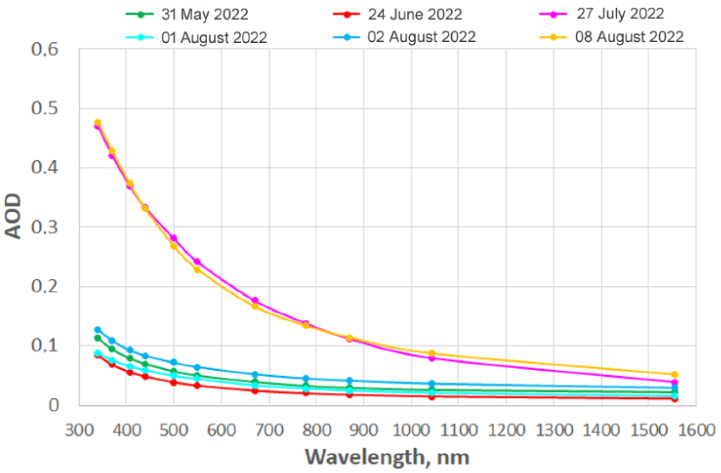
The regular measurements of the atmospheric aerosol properties were launched in 2022 and carried out from May to August. In contrast to areas of seas and oceans with powerful convection, inland waters of temperate latitudes, even in summer, often turn out to be partially covered by clouds. Therefore, only 6 days of measurements were selected for further analysis, when the most cloudless Sentinel-3/OLCI images were obtained: 31 May, 24 June, 27 July, 1 August, 2 August, and 8 August.

2.2. Field Measurements of the Aerosol Optical Properties and Data Processing

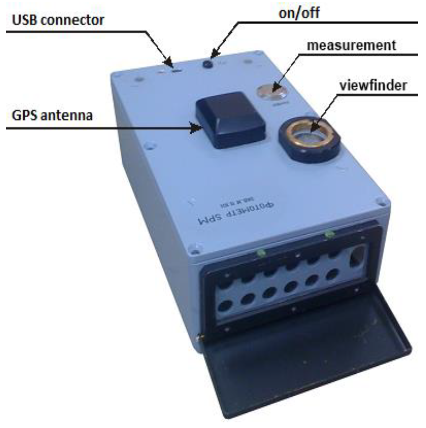
Measurements of the main optical properties of the atmosphere over the Gorky Reservoir were carried out from May to August 2022 using an SPM handheld sun photometer developed at the Institute of Atmospheric Optics, Tomsk, Russia (Figure 1). The SPM photometer registers signals coming from the sun with a cloudless sky in 10 spectral channels 339, 373, 439, 499, 673, 871, 939, 1044, 1555, and 2139 nm [22,23,24,25,26]. Thus, SPM has an advantage in spectral range and the number of measuring channels (filters) in comparison with AERONET sun photometers. The SPM photometer is assembled on a modern elemental base, and its photoelectric optoelectronic circuit is similar to the stationary SP-9 photometer, which conducts measurements in a normal mode. The SPM photometer has a built-in software interface with a computer and is provided with software that allows retrieving the AOD and precipitable water.
The photometer was pointed at the sun by the operator from the “hands-on” position, using a viewfinder. Measurements were taken every hour for several minutes. The registered spectral sun radiation (together with GPS coordinates, measurement time, pressure, and temperature) was accumulated in a digital form in the flash memory of the device and then transferred via the USB port to a personal computer to calculate the AOD and precipitable water. Processing of the obtained data (calculation of physical characteristics) was performed using a special computer program that provides automatic data filtering [22].
Under normal operating conditions and calibration data, the error in determining the AOD is 0.01–0.02, and the moisture content of the atmosphere is 0.1 g/cm2. The methods of calibration and calculation of the desired characteristics are described in [23,24,25,26].

2.3. Determination of the Type of Aerosols over the Studied Regions

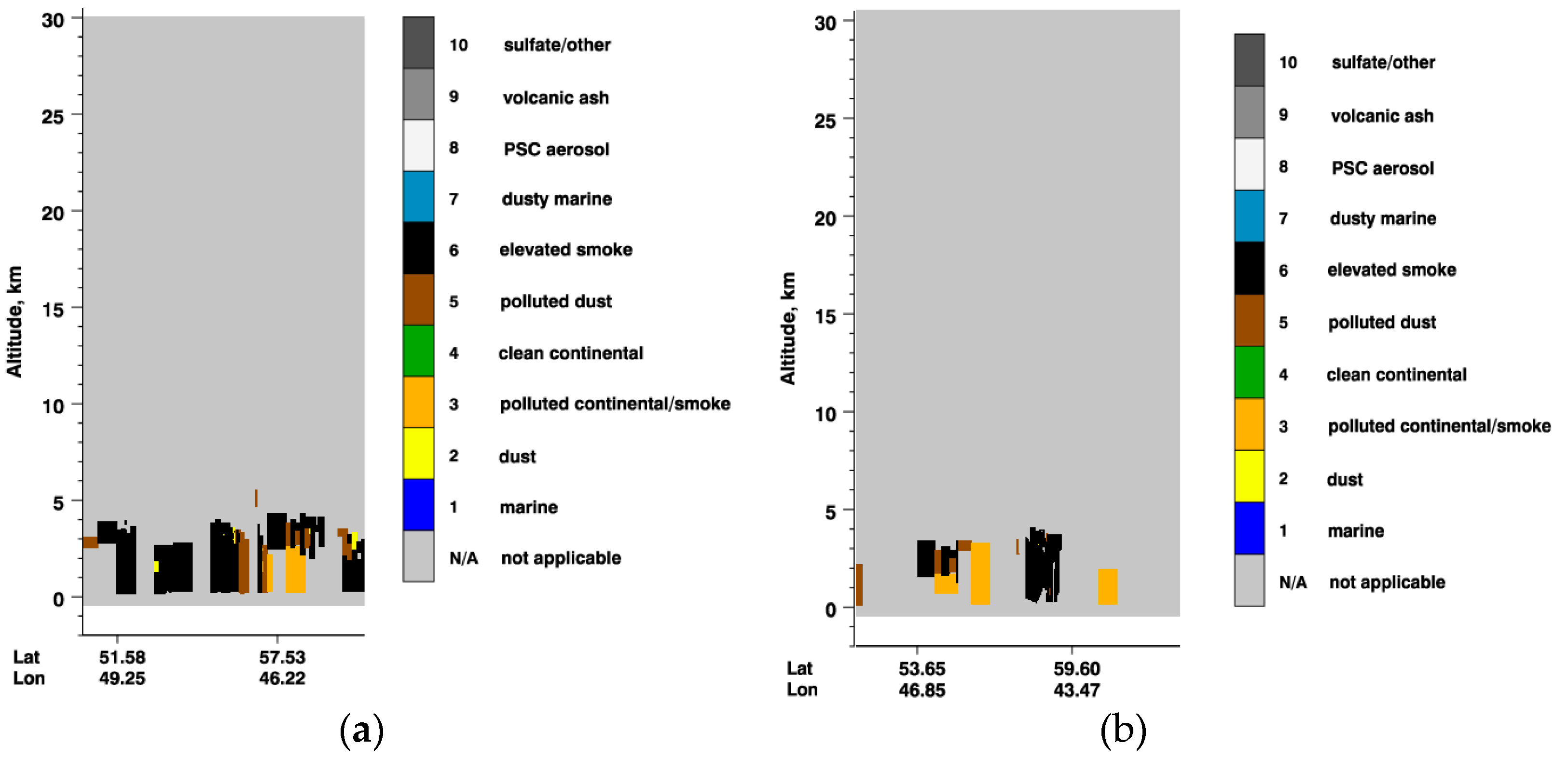
In order to determine the type of aerosols, we analyzed the data from CALIPSO (Cloud-Aerosol Lidar and Infrared Pathfinder Satellite Observation, https://www-calipso.larc.nasa.gov/ (accessed on 28 November 2022)), an American–French research satellite launched as part of the EOS (Earth Observing System) by NASA and designed to study the cloud cover of the Earth. The main goal of CALIPSO is to conduct global measurements of aerosols and clouds. The CALIPSO payload consists of three co-aligned nadir-viewing instruments; the Cloud-Aerosol Lidar with Orthogonal Polarization (CALIOP), the Imaging Infrared Radiometer (IIR), and the Wide Field Camera (WFC). The types of aerosols are specified by the value of the integral backscattering coefficient and by the value of the particle depolarization coefficient. The specified aerosol types include smoke (from forest fires), dust, polluted dust (a mixture of dust and smoke), polluted continental, and pure continental aerosol. Each type of aerosol is characterized by a set of lidar ratios at wavelengths of 532 and 1064 nm [27].

2.4. Determination of Atmospheric Aerosol Sources

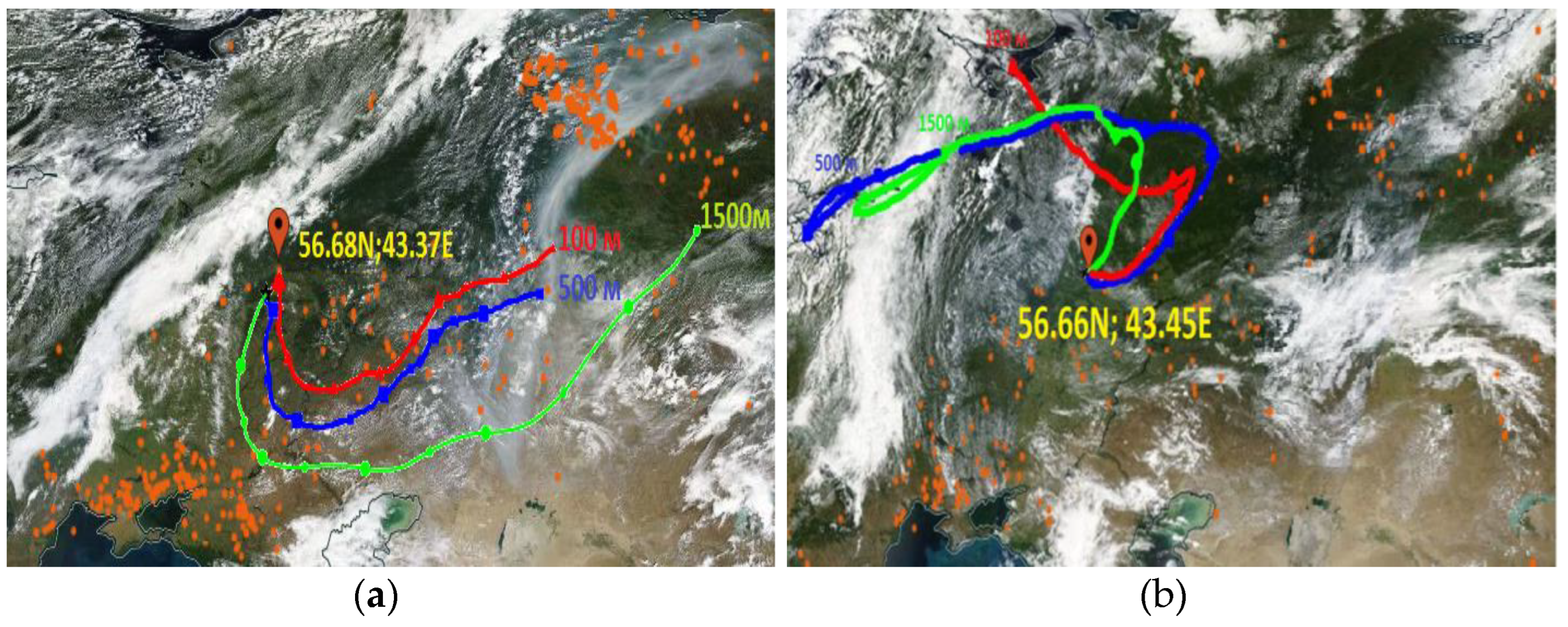
Atmospheric aerosol sources were determined using the HYSPLIT model (Hybrid Single-Particle Lagrangian Integrated Trajectory model, https://www.ready.noaa.gov/HYSPLIT.php (accessed on 28 November 2022)). This model provides back trajectory analysis to identify the origin of air masses and establish source–receptor relationships. The data of the model are also employed in various models describing the atmospheric transport, dispersion, and deposition of pollutants and hazardous materials. The default model configuration assumes a 3D particle distribution (horizontal and vertical) [28].

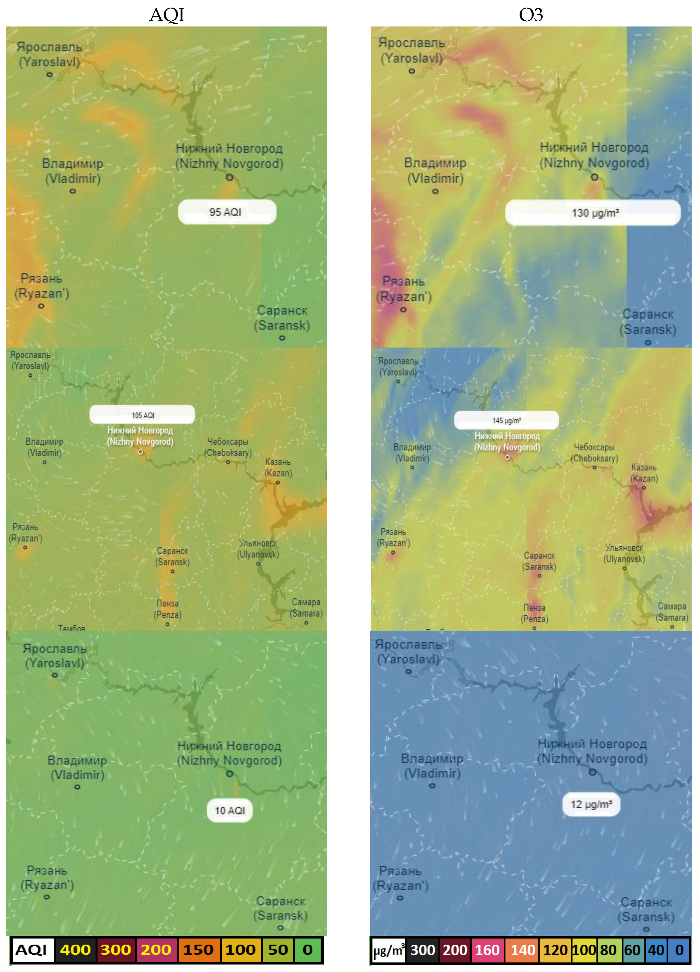
2.5. Air Quality Analysis

Harmful substances, including carbon dioxide, ozone, and methane, can lead to significant deterioration of human health. In this paper, two parameters characterizing the content of harmful substances in the atmosphere, namely air quality index (AQI) and ozone content (O3), were analyzed. The air quality index is used by all environmental government agencies in the world to inform the public about the level of air pollution, as well as to predict air pollution. Values above 300 represent unsatisfactory (dangerous to humans) air quality, values from 200 to 300 represent very unhealthy air quality, from 150 to 200, unhealthy, from 100 to 150, unhealthy for sensitive groups, and below 100 or even below 50, good air quality.
Ozone is one of the AQI criteria used in air quality assessments. It is generally accepted that a safe exposure is 0–100 µg/m3 (within 8 h). Different countries have their own air quality index that meets national standards.
These parameters were estimated using the SILAM (System for Integrated Modeling of Atmospheric Composition, https://silam.fmi.fi/ (accessed on 28 November 2022)) as the system of integrated modeling of the atmosphere composition. According to the SILAM model [29], the sources of aerosol activity include sea salt, wind-blown dust, pollen, natural volatile organic compounds, radionuclides (nuclear fission products), and smoke determined by the IS4FRIES fire information system. The SILAM is widely used to study the effects of forest fires, volcanic eruptions, dust transport, and other natural and man-made disasters on atmospheric pollution.

2.6. Estimation of the AOD Accuracy of Level-2 SYN AOD Products

Based on a series of measurements of aerosol under the Gorky Reservoir, we tried to evaluate the accuracy of AOD retrieval on Sentinel-3/OLCI images: the global aerosol characteristics Level-2 SYN AOD products (present subsection) and OLCI Level-2 Water Full Resolution products (next subsection).
The Sentinel-3 SYN are Level-2 products that are obtained using a combination of the data of OLCI (Ocean and Land Colour Instrument) and SLSTR (Sea and Land Surface Temperature Radiometer) instruments. The SYN products can be classified into three main types: (i) surface reflectance and aerosol parameters over land, (ii) vegetation-like products, and (iii) aerosol characteristics over land and sea.
Level-2 SYN AOD is a set of products of aerosol characteristics for a cloud-free atmosphere over both land and ocean projected on a 4.5 km grid (superpixel). Algorithms for aerosol retrieval are described in detail in [30].
In order to estimate the accuracy of the AOD and the Angstrom exponent, the SYN AOD data were selected from the pixel where the station coordinates fell and compared with the in situ measurements. The accuracy of the products was evaluated using the relative error and the linear regression coefficient.
For the mentioned six dates when field measurements of aerosol were carried out, 6 SYN AOD images were selected (5 for Sentinel-3A and 1 for Sentinel-3B). Measurements were conducted over water for three days (31 May, 1 August and 8 August 2022) and overland for two days (24 June and 27 July 2022). The SYN AOD images were downloaded from the Copernicus Open Access Hub (https://scihub.copernicus.eu/dhus (accessed on 28 November 2022)).

2.7. Estimation of the AOD Accuracy of OLCI Level-2 Water Full Resolution Products

OLCI Level-2 Water Full Resolution (OL_2_WFR) products are outputs from the OLCI Level-2 processor and contain water and atmospheric geophysical products, a complete list of which is available on the website ESA (https://www.esa.int/ (accessed on 28 November 2022)). They were obtained following ESA’s standard atmospheric correction procedure combining two approaches: (i) a baseline AC, which is a combination of the “black water” approach with the bright pixel atmospheric correction [6,31], and (ii) an alternative AC in which atmospheric parameters and water-leaving reflectance are inverted through neural networks [32].
The list of atmospheric geophysical products includes aerosol optical depth at 865 nm (AOD865) and spectral dependency of AOD between 779 and 865 nm (Angstrom exponent α). For dates when AOD measurements were performed in the Gorky Reservoir, 11 OL_2_WFR images were downloaded (6 for Sentinel-3A and 5 for Sentinel-3B) from the EUMETSAT Data Store using the Product navigator web service (https://navigator.eumetsat.int (accessed on 28 November 2022)).
The analysis of the images was carried out as follows.
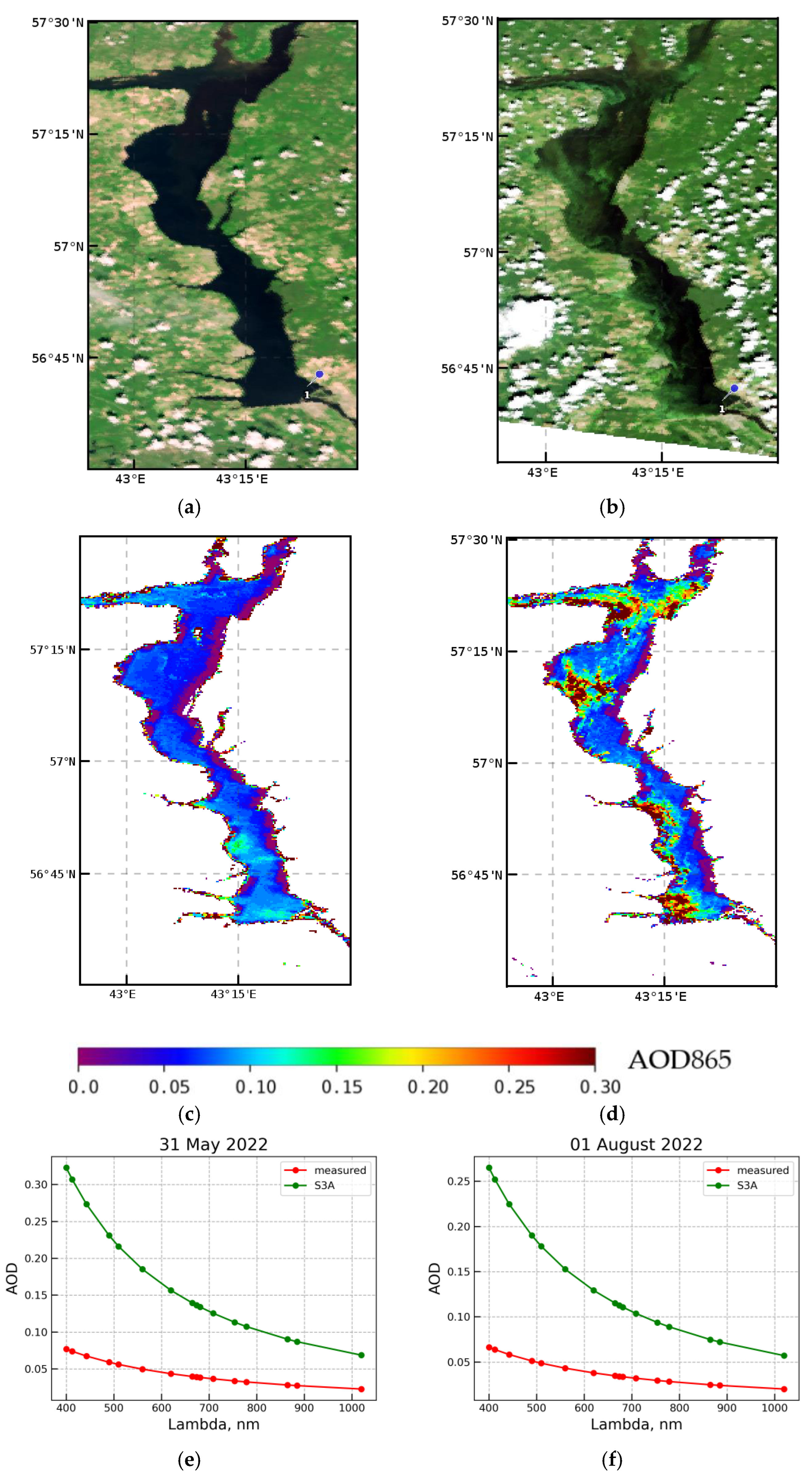
1. For each image, an RGB composite, which was visually compared with the AOD865 field, was made. In cases where the distribution of AOD865 repeated the features of the radiance of water pixels, it can be concluded that the prediction of the water-leaving radiance in the NIR bands and the separation of aerosol radiance during the atmospheric correction were performed incorrectly. The aerosol component of radiance was overestimated due to the inclusion of part of the water radiance.
2. For three dates when AOD measurements were made over water, OL_2_WFR aerosol parameters averaged over a 3 × 3-pixel box around the station were compared with field measurements. The AOD on the central wavelength of OLCI bands was calculated using the relation
AOD ( λ i ) = AOD ( λ 0 ) ( λ 0 / λ i ) α ,
where λ i is the central wavelength of the Sentinel-3/OLCI spectral band, α is the Angstrom exponent, and λ 0 is the reference wavelength for OL_2_WFR (865 nm).

2.8. Accuracy Estimation of the Conventional AC and AC with a Fixed AOD Based on In Situ Data

As mentioned above, atmospheric correction of optical images conventionally uses two infrared bands to determine the aerosol radiance, while the parameters of atmospheric aerosol are determined independently in each pixel of an image, i.e., they are spatially variable. Previously, in the Gorky Reservoir, we employed the AC algorithm with a fixed AOD [18], which showed good results in Rrs recovery. Below, we present the results of a comparison of AC with a variable aerosol, determined from the image itself without involving additional information, and AC with a constant aerosol, the parameters of which were specified by the measured AOD spectrum. Although the assumption of the spatial invariance of atmospheric aerosol is extremely conditional as shown by our results [18] within the area of interest (10 km × 10 km), such an approach can allow retrieving of Rrs from satellite images with high accuracy.
Atmospheric correction of Sentinel-3/OLCI images of both types was performed due to the l2gen processor in NASA Goddard Space Flight Center seaDAS v.8.2 software (https://seadas.gsfc.nasa.gov/seadas_license/ (accessed on 28 November 2022)). In the common NASA approach [5], the aerosol reflectance is calculated from two NIR bands 779 nm and 865 nm (hereafter referred to as ac-2) and then extrapolated to visible bands, together with an iterative procedure for calculating the water-leaving reflectance in NIR bands [33] (option aeropt = −2). AC with a fixed AOD (option aeropt = −8) was performed by specifying the AOD spectrum based on in situ measurements (hereafter referred to as ac-8).
A quantitative assessment of the AC accuracy by comparing the retrieval Rrs with in situ measured ones was not performed in the present study. Such validation is related to a laborious process of conducting and accumulating in situ radiometric measurements; therefore, it is the subject of our future research. As a result, the assessment of the AC accuracy was carried out only at a qualitative level, i.e., by estimating the number of negative values of the Rrs.
The chlorophyll algorithm failure (CHLFAIL) quality flag was chosen as a criterion expressing the quantity of negative Rrs in bands used to determine the chlorophyll a concentration. The l2gen processor uses the OC4 algorithm, which is the fourth-order polynomial relationship between a ratio of Rrs and chlorophyll a
log 10 ( Chl   a ) = a 0 + i = 1 4 a i ( log 10 ( R rs ( λ blue ) R rs ( λ green ) ) ) i ,
where R rs ( λ blue ) is the highest Rrs value at wavelengths of 443 nm, 490 nm, and 510 nm; R rs ( λ green ) is the Rrs at a wavelength of 560 nm; and a 0 and a i are the polynomial coefficients.
Thus, the CHLFAIL flag means that Rrs is not specified or negative at least at one of the wavelengths. The proportion of pixels, marked with the CHLFAIL flag, was calculated as pixel number with the CHLFAIL flag divided by the total number of valid pixels (VALID) (Figure 2). The latter were calculated as the difference between the number of water pixels (WATER = not LAND flag) and pixels with probable cloud pollution (CLDICE = probable cloud or ice contamination), stray light (STRAYLIGHT), high top-of-atmosphere (TOA) radiance (HILT), and high sun glint (HIGLINT) flags. It should be noted that due to the high radiance, a significant part of the water pixels along the banks of the Gorky Reservoir is also marked with the CLDICE flag (Figure 2).
In addition to pixels with the CHLFAIL flag, the number of pixels with the CHLWARN (chlorophyll a out-of-bounds <0.01 or >100 mg/m3), ATMWARN (atmospheric correction is suspect), and ATMFAIL (atmospheric correction failure) flags are also given. A detailed analysis of the pixels marked with these flags has not been performed, but they are also presented as additional markers for comparing the two types of AC.
AC was performed on 11 radiometrically calibrated, geo-referenced Level-1B full-resolution OL_1_EFR images (6 for Sentinel-3A and 5 for Sentinel-3B) downloaded via the Copernicus Open Access Hub (https://scihub.copernicus.eu/dhus (accessed on 28 November 2022)).

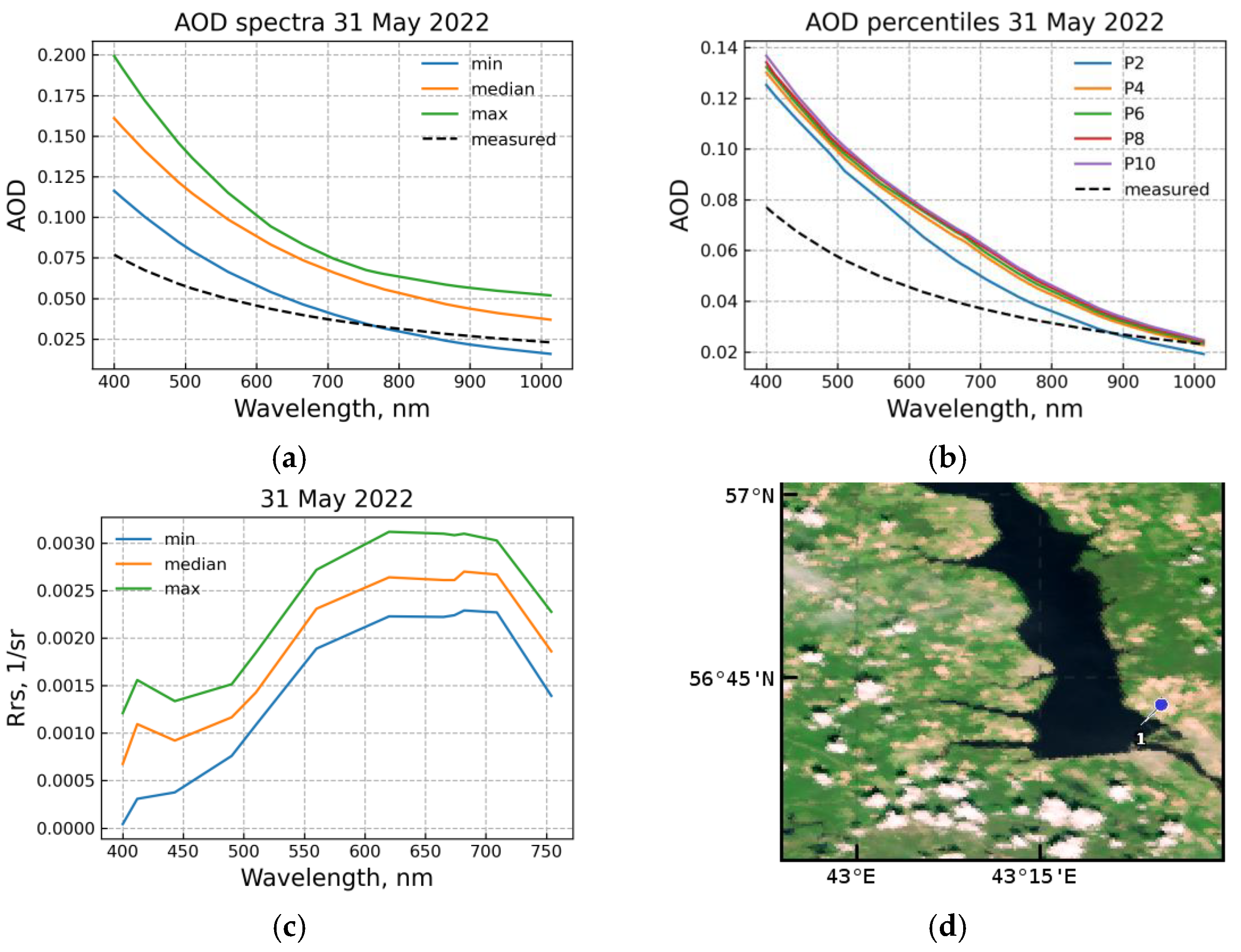
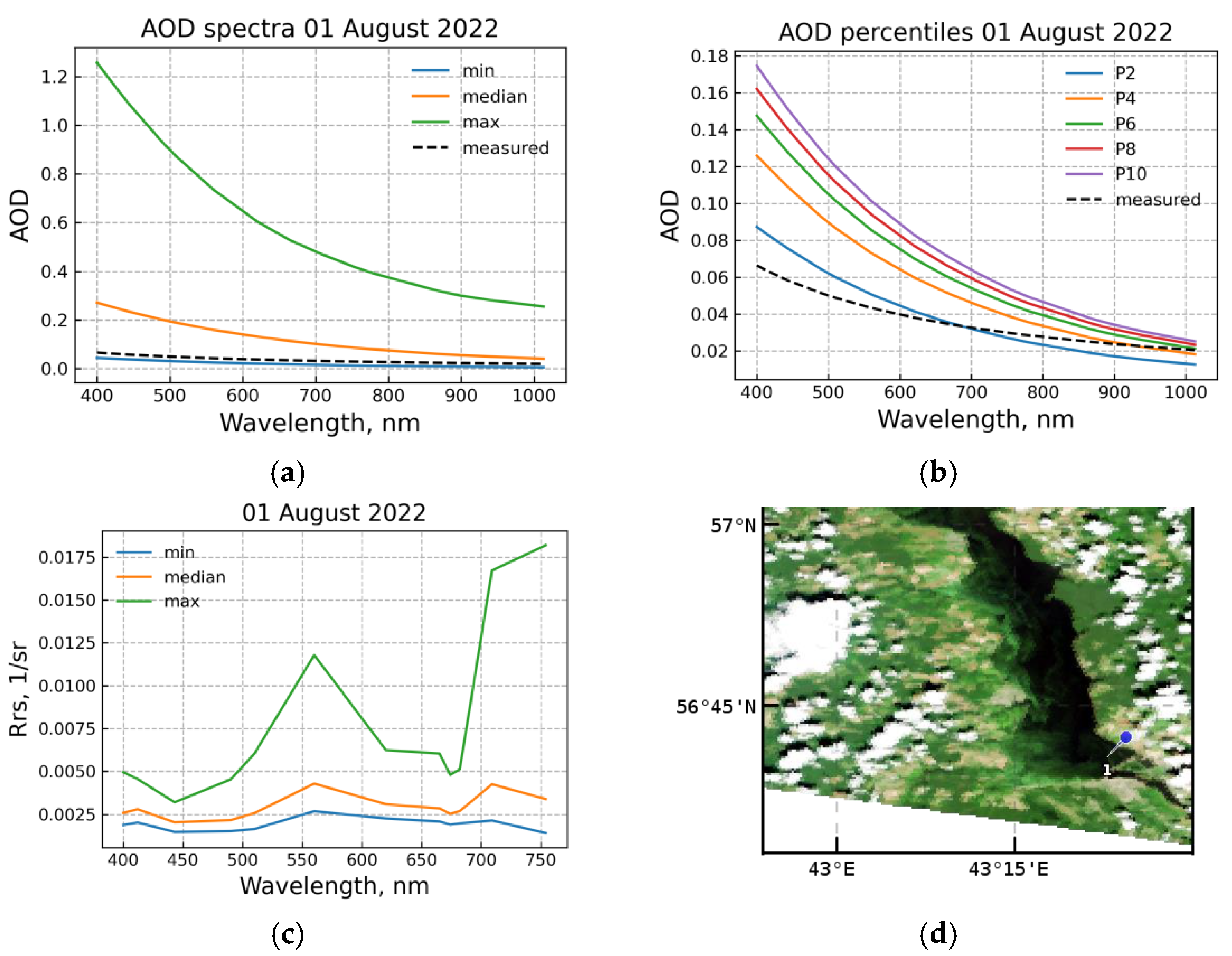
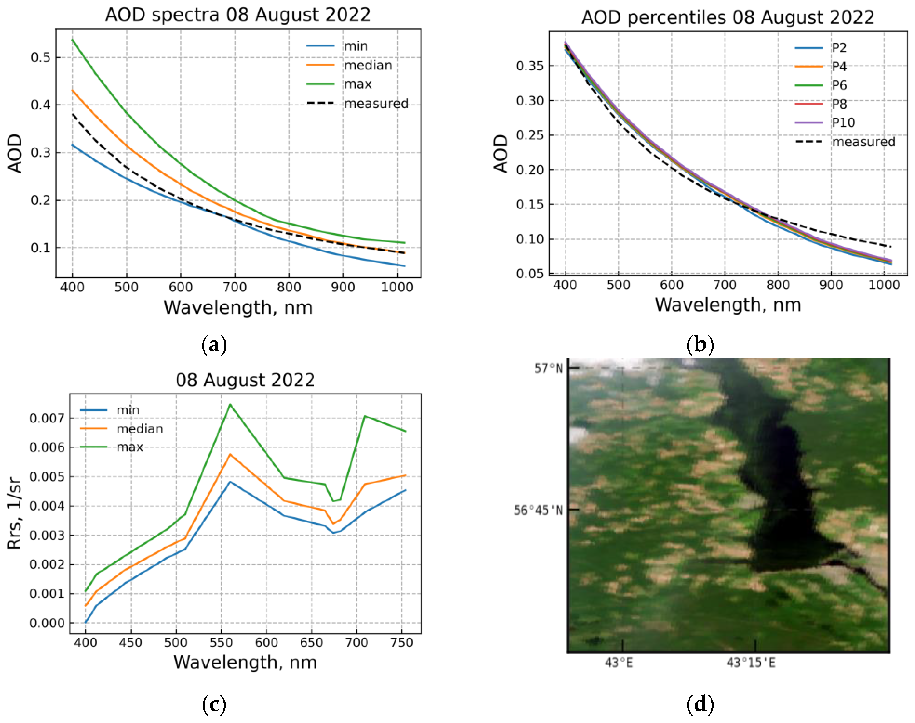
2.9. Analysis of AOD Spectra Obtained as a Result of Conventional Atmospheric Correction

Although the AOD obtained using conventional AC in productive waters is significantly overestimated, it is possible to find an area with relatively clean water on the image, where the errors in determining the AOD are minimal. Such areas can be determined, for example, by the minimum values of water radiance in one of the spectral bands [34,35]. In [
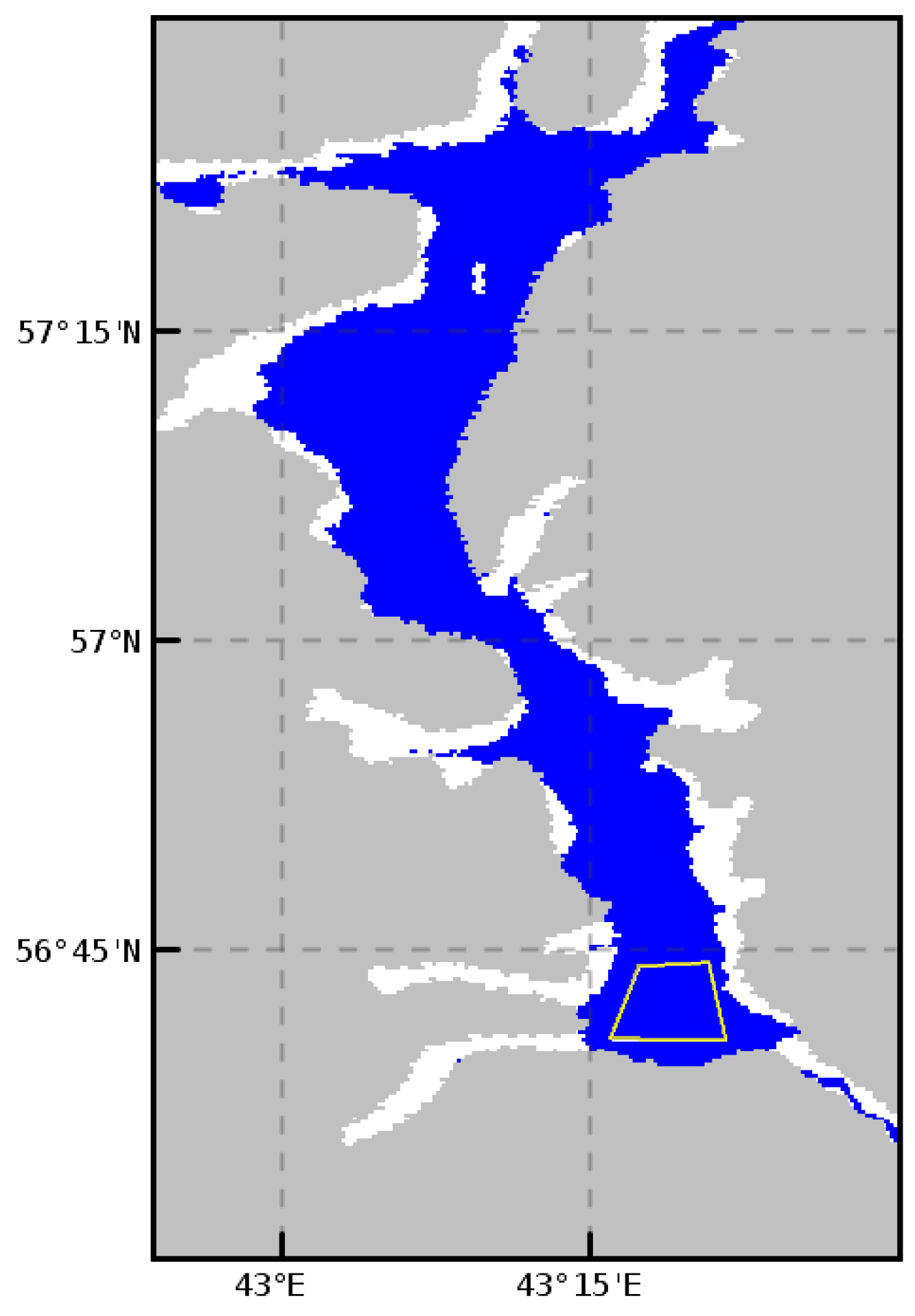
18], the clean water area was determined by the fifth percentile of the AOD distribution. This approach is analyzed in the present paper. For this purpose, the first 10 percentiles of the AOD distribution were plotted according to the ac-2 data and compared with the measured AOD. The sample included only pixels that fell into the test region indicated by the yellow quadrangle in Figure 2. The methods for selecting valid pixels are described in detail in Section 2.8.
Furthermore, for all images, the percentile that most closely describes the spectrum of the measured AOD (AOD for “clean” water) was selected. The percentile was employed for AC with fixed AOD of selected Sentinel-3/OLCI images using an l2gen processor (option aeropt = −8). The Rrs values obtained during this AC in the test region (Figure 2) were compared with the Rrs retrieved on a base of the measured AOD spectrum (Section 2.8). For this purpose, we calculated the relative error for Rrs averaged over the test region.

3. Results

3.1. Estimation of AOD Accuracy of Level-2 SYN AOD Products

Figure 3 shows the AOD spectra according to the Level-2 SYN AOD (hereinafter referred to as SY_AOD) and in situ measurements taken on 27 July and 1 August 2022. In addition to AOD determined in the superpixel, AOD uncertainties equal to one standard deviation are also given [30].
A high aerosol load with AOD (550 nm) of 0.242 was observed on 27 July and a low one with AOD (550 nm) of 0.045 on 1 August. Although SY_AOD is overestimated in the first case and underestimated in the second one, this behavior is not confirmed by other dates. The relative AOD error at a wavelength of 550 nm for individual dates varied from ±0.4 to 2.2 (Table 1), and the average value of 0.3 for all selected images (plus sign means that SY_AOD exceeds the measured AOD). Despite this, for three out of six images, the measured AODs are within the confidence interval of the SY_AOD estimates.
The AOD uncertainties are minimal at a wavelength of 1610 nm and increase towards the visible and SWIR range of the spectrum, with maximum values at wavelengths of 442 and 2250 nm. Probably, high AOD uncertainties indicate a large spatial inhomogeneity of the aerosol optical properties determined within the superpixel. In some cases, the uncertainties even exceeded the range of variability of the AOD themselves and amounted to 1–2. For this reason, two images were excluded from further analysis.
For the remaining four images, linear regressions were plotted, and relative errors were calculated for AOD at a reference waveband (550 nm). These data are presented in Table 1 and in Figure 4. Two measurements were taken for cases with small (AOD~0.05) and large (AOD~0.23) aerosol loads. Higher AOD uncertainties are characteristic of a large aerosol load (Table 1). Linear regressions based on the SY_AOD estimates, upper, and lower bounds of the confidence interval are shown with green, red, and brown lines, respectively. Unfortunately, the correlation coefficients are too low (with the exception of the regression on the upper bound of the confidence interval) to indicate any relationship between SY_AOD and the measured data.

3.2. Evaluation of AOD Accuracy of OLCI Level-2 Water Full Resolution Products

Figure 5 shows the AOD distribution at a reference wavelength of 865 nm according to OL_2_WFR data on 31 May and 1 August 2022. These dates are typical of situations where the optical properties of water are determined by suspended matter (31 May) and a high content of phytoplankton (1 August). At the same time, due to the location of river discharges and the peculiarities of the reservoir hydrology, suspended matter and phytoplankton (as a passive matter) are transferred downstream, being redistributed along the right bank of the reservoir and accumulating near the hydroelectric dam. This feature is hardly notable due to low contrasts on the RGB composite on 31 May (Figure 5a) but is clearly visible on 1 August (Figure 5b).
AOD865 according to OL_2_WFR for both situations repeats the features of the distribution of more turbid waters; higher values are located near the right bank, in the area of river discharges, and near the dam (Figure 5c,d). The values of AOD865 also raise doubts; on 31 May near the dam they are 0.085–0.115, and on 1 August, 0.115–0.175, and they exceed 0.3 in the areas of concentration of cyanobacteria. These values are significantly overestimated due to an incorrect determination of the water-leaving radiance in the NIR bands. Areas with physically plausible AOD865 values (indicated by purple color) are located along the left bank of the reservoir and are almost identical for the two images, except for the places where an increased concentration of cyanobacteria was observed.
A comparison of AOD865 spectra from OL_2_WFR with in situ measurements is shown in Figure 5e,f. Positions of the measurement stations are shown in Figure 5a,b. The spectra of AOD865 from OL_2_WFR are much steeper due to the large Angstrom exponents; the measured values were 1.2978 and 1.2698, and the satellite ones were 1.6523 and 1.6391 for 31 May and 1 August, respectively. The excess of AOD at the reference wavelength of 865 nm according to OL_2_WFR turned out to be three times greater. Similar features of AOD865 from OL_2_WFR were observed for all six selected images.

3.3. Accuracy Estimation of the Conventional AC and AC with a Fixed AOD Based on In Situ Data

The number of valid pixels (VALID) marked with the CHLWARN, CHLFAIL, ATMWARN, and ATMFAIL flags, as well as the proportion of pixels with the CHLFAIL flag (PART CHLFAIL), calculated based on the results of AC ac-2 and ac-8 for Sentinel-3A/OLCI and Sentinel- 3B/OLCI are given in Table 2, Table 3, Table 4 and Table 5, respectively.
The lake part of the Gorky Reservoir (100 km long) accounts for about 12,500 pixels of Sentinel-3/OLCI images (Figure 2). About one-third of these pixels are near-shore regions with high radiance, which are masked as clouds before the AC. As a result, about 8000–8500 valid water pixels for which Level-2 products can be obtained remain. In the presence of clouds, the number of actual pixels decreases even more, and for some images, it was reduced to 2000–4000.
As can be seen from Table 2 and Table 4, the number of pixels with the ATMWARN flag is more than 95%, and with the CHLFAIL flag, 40–60% during the period of the absence of algal blooms (31 May and 24 June) and 70–100% in July and August when an active bloom of cyanobacteria takes a place. Based on this, it can be concluded that the aerosol radiance is significantly overestimated which leads to 40–100% of the values of Rrs being negative, at least in the blue and green bands of the OLCI sensor when using AC ac-2.
When employing the AC with a fixed AOD ac-8, based on the in-situ measurements (Table 3 and Table 5), the proportion of pixels with the CHLFAIL flag turn to zero, which indicates a qualitative improvement in Rrs retrieval. In this case, not only negative values disappear, but also the shape of the Rrs spectrum is aligned. The Rrs except for the 413 and 430 nm bands (Figure 6c, Figure 7c and Figure 8c) is typical of the reservoir [18,36].

3.4. Analysis of AOD Spectra Obtained as a Result of Conventional AC

Figure 6a, Figure 7a and Figure 8a show the minimum, median, and maximum AOD spectra obtained using AC ac-2 in the test region (Figure 2) on 31 May, 1 August, and 8 August 2022. In most cases, the measured AOD spectrum is located between the minimum and median values (Figure 7a and Figure 8a). Only in two of the eight images (5 S3A and 3 S3B) is the measured AOD spectrum less than the minimum AOD obtained as a result of ac-2 (Figure 6a). This indicates that in the images of highly productive reservoirs it is possible to identify an area of clean water, where the atmospheric parameters are determined correctly or are close to true values. Such AOD spectrum over clean water can be used in AC with a fixed AOD.
Figure 6b, Figure 7b and Figure 8b show how the measured AOD spectra match with the first ten percentiles of AOD obtained using ac-2. The first ten percentiles of AOD (P10) have a different scatter among themselves. In most cases, the difference between the second P2 and the fourth P4 percentiles was the biggest, and after P4, the other percentiles were more closely spaced. As the percentile increased, the Angstrom exponent (the AOD spectral slope) also increased. In the case of a high aerosol load (Figure 8b), on the contrary, a dense arrangement of all ten percentiles was observed.
Thus, we conclude that the second percentile P2 spectrum corresponds more to the measured AOD spectrum in most situations. After that, we performed AC of Sentinel-3/OLCI images with fixed AOD using P2 spectrum. Furthermore, considering the measured AOD as the true value, we calculated the relative error of Rrs in different spectral bands (Table 6).
Naturally, the values of the relative error depend on the proximity of P2 to the measured AOD, as evidenced by the range of relative errors. The minimum values do not exceed 5% on the spectral bands of 560–754 nm and increase to 20% on the bands of 400 and 412 nm. The maximum values already reach 35% and 73% on the same bands.

3.5. Estimates of Aerosol Composition and Transport Sources

The results of AOD recovery from the measurements using the sun photometer are shown in Figure 9. As can be seen, four of the six dates correspond to relatively low AOD values, while increased AOD values (relative to the average monthly) were recorded over the entire spectral range of measurements on 27 July and 8 August. The monthly average value of the AOD at a wavelength of 500 nm (AOD(500)) was 0.17 for July, while the daily average AOD(500) was 0.28 for 27 July 2022. The average monthly AOD(500) was 0.18 for August, while the average daily AOD value was 0.27 for 8 August 2022. For these days, analysis of the results of assessing the contribution of large and small aerosol particles to the total distribution of AOD(500) showed that the aerosol mainly consists of a finely dispersed fraction (85%). Accordingly, the increase in AOD values is due to the presence not of large aerosol particles, but of a large number of small particles with strong absorbing properties. These particles include desert dust particles and smoke. This statement is consistent with the results of modeling the reverse trajectories of air flows for 8 August 2022, presented in Figure 10a. According to Figure 10a, smoke aerosol moved into the study area from the Orenburg region and the Urals, where extensive fires were registered. A different situation was observed for the second date of observation of elevated AOD values, namely 27 July 2022. The return trajectories constructed for vertical profiles of 100, 500, and 1500 m (Figure 10b) did not reveal any source of absorbing aerosol (dust haze or smoke) in the west and northwest. Therefore, the analysis of aerosol types for the study region was carried out using the CALIPSO data. The results of this analysis for both dates are shown in Figure 11. One can see the presence of large amounts of smoke on 8 August, as well as polluted dust and smoke in the atmosphere over the study region on July 27.
The results of estimating the AQI index and ozone concentration according to the SILAM model are presented in Figure 12 for dates with elevated AOD values, as well as when low AOD values were obtained, for example, on 24 June 2022. As can be seen in Figure 12, the values of air quality parameters for this date, which correspond to the minimum content of harmful substances in the atmosphere, are observed, while for 27 July and 8 August, the values of two parameters are close to dangerous for human health.

4. Discussion

Information on the parameters of atmospheric aerosol is important in solving a wide range of problems related to the study of processes occurring in the atmosphere (radiation mode, heat balance, climate change, etc.) and affecting the ecology of the environment as a whole. Since aerosols make a significant contribution to the reflection, scattering, and absorption of solar radiation, information about their parameters is also relevant for studying the optical properties of the waters of the oceans, seas, and freshwater bodies, which are directly related to both the ecology of waters and its bioproductivity.
In remote-sensing ocean color radiometry, about 90–95% of the signal in the visible and NIR regions of the spectrum is formed by the atmosphere. Therefore, the accuracy of estimating the water-leaving signal critically depends on the correctness of determining the aerosol parameters and the aerosol radiance. The existing approach to the atmospheric correction of satellite optical images involves determining the aerosol contribution from radiance in two NIR bands. However, for turbid or highly productive waters, which include most of the coastal areas of the seas and freshwater bodies, this approach turns out to be inefficient, since due to the significant water-leaving radiance in the NIR, it is not possible to correctly separate the aerosol component.
Based on a series of measurements of aerosol under the Gorky Reservoir, we tried to test two concepts for atmospheric correction with fixed AOD of Sentinel-3/OLCI images. The first one assumed that additional third-party data about AOD can utilize AC to improve its accuracy in Case-2 water. As an example, we considered the global product Level-2 SYN AOD of aerosol characteristics and OLCI Level-2 Water Full Resolution products. The second concept was that the AOD spectrum can be determined from the image itself without involving additional data under the clean water area.
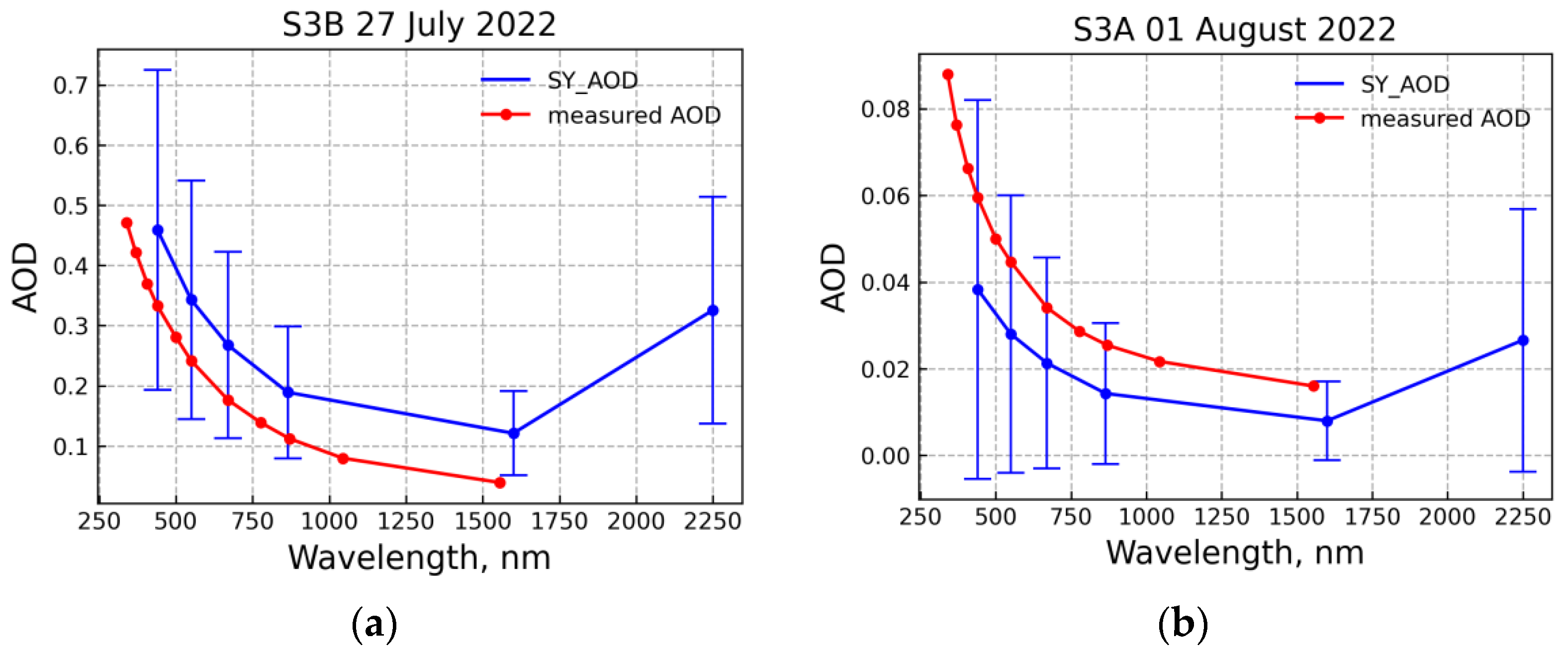
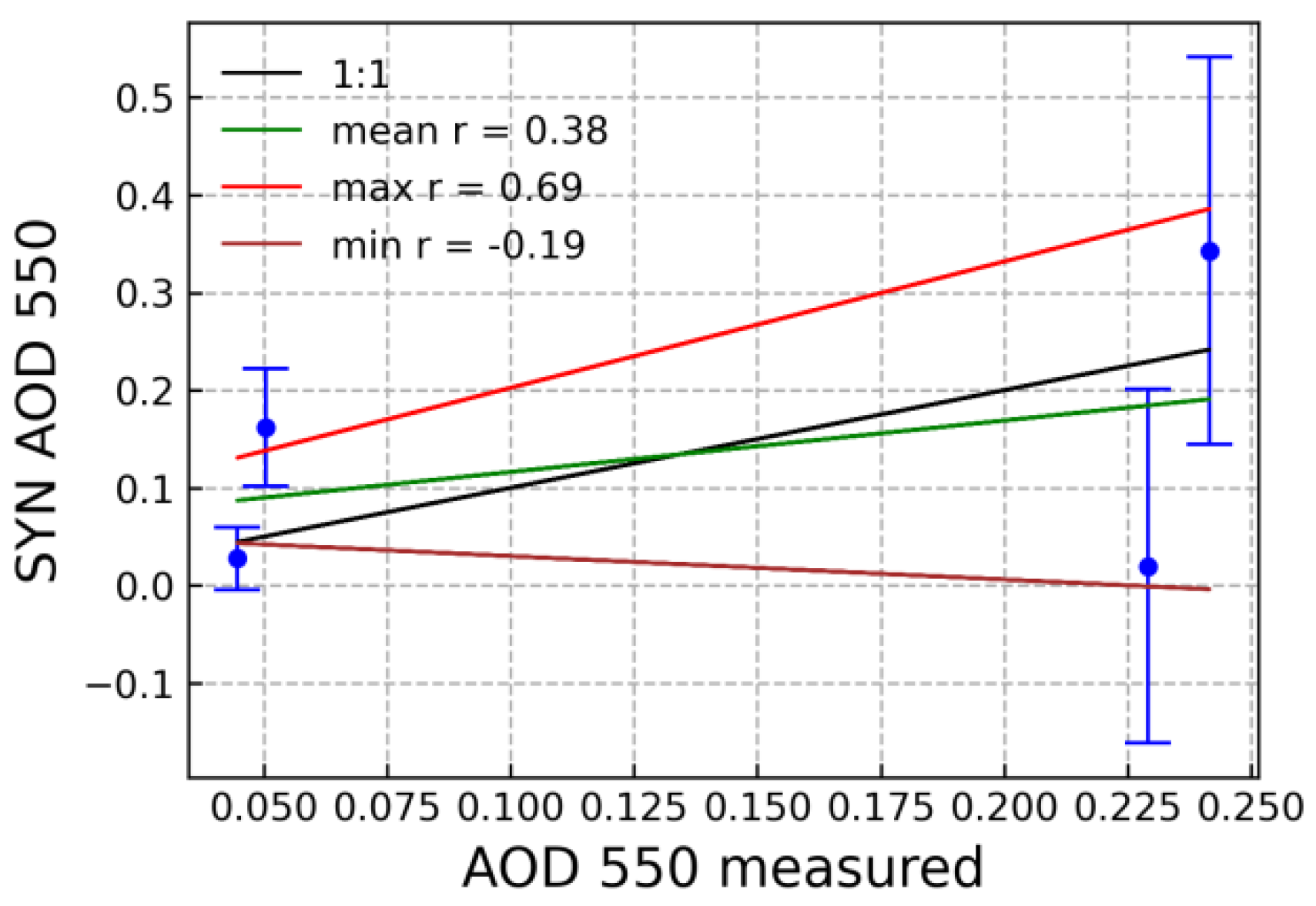
Comparing measured AOD with SY_AOD data, we did not find any relationship between these values (the linear correlation coefficient was 0.38). Although the small number of measurements does not enable us to conclude with certainty about the accuracy of the SY_AOD products, the average value of the relative error of the AOD at a reference wavelength of 550 nm was 0.3, while the scatter was quite large from ±0.4 to 2.2. Despite the fact that for three of the six images, the measured AODs were within the confidence interval of the SY_AOD estimates, the confidence interval was high and ranged from 100% or more of the estimated value. The wide confidence intervals are probably the result of the strong spatial aerosol variability within a 4.5 km superpixel, especially since we observed an increase in the AOD uncertainty in cases of higher aerosol loading. Unfortunately, the listed features do not make it possible to draw final conclusions about both the accuracy of the SY_AOD products and the possibility of their use in AC with a fixed AOD and require further study.
Estimates of the AOD at 865 nm (AOD865) and the Angstrom exponent from OL_2_WFR data, which were obtained as a result of conventional AC using two NIR bands, eloquently demonstrated the inefficiency of this approach in the case of productive inland waters of the Gorky Reservoir. In all selected images, the AOD865 repeated the features of the distribution of optically active components in water, which, due to the circulation features, are concentrated near the right bank of the reservoir and near the hydroelectric dam. This was observed both in cases of the dominance of cyanobacteria and in cases where the optical properties were determined by dissolved organic matter and mineral suspension.
In all images, the AOD865 exceeded the measured AOD by more than three times, and the AOD spectra were much steeper due to higher Angstrom exponents. Such a large overestimation of the aerosol parameters led to negative Rrs on the bands of 400–560 nm and sometimes up to 680 nm.
When analyzing the AOD865 distribution, an interesting feature was found; the minimum (physically plausible) values were located along the left bank of the reservoir. Their location remained almost constant for most of the considered images. Perhaps, due to the hydrological features of the reservoir and the wind mode, areas with relatively clean water are formed in these places in which the aerosol parameters are determined with smaller errors. In the future, more attention should be paid to the study of this feature.
Studying the second concept, it was first shown that AC with a fixed AOD based on in situ measurement allows achieving qualitatively better results in retrieval of Rrs. Using conventional AC (ac-2), in which the aerosol parameters are calculated in each pixel of the image from two NIR bands, the aerosol radiance is significantly overestimated. As a result, from 40 to 100% of water pixels are marked with the CHLFAIL quality flag. This, in turn, shows that Rrs is negative at least in the blue and green bands used to determine the chlorophyll a concentration. During the cyanobacteria bloom, the number of pixels marked with the CHLFAIL flag increases, which also confirms the low accuracy of estimating the water-leaving radiance in the NIR bands and the separation of the aerosol component in waters with high productivity.
The use of the measured AOD spectrum in the AC made it possible to obtain realistic Rrs values typical for the reservoir by reducing to zero the number of pixels with the CHLFAIL flag. In this case, the number of pixels marked with other quality flags (CHLWARN, ATMWARN, and ATMFAIL) was also significantly reduced. Although this approach is based on the hypothesis of the constancy of the AOD, which will be fulfilled in limited cases on small spatial scales, it enables one to obtain estimates of Rrs, the accuracy of which can later be estimated by radiometric measurements. Having estimates of Rrs and knowing their accuracy, one can try to develop an algorithm for retrieving the chlorophyll a concentration, considering the regional hydro-optical features of the reservoir. It stands to reason that the work in this direction is impossible when the Rrs retrieved as a result of AC is negative.
Next, we analyzed the totality of the AOD spectra obtained as a result of conventional AC ac-2. In most cases, the measured AOD spectrum was between the minimum and median AOD spectra of ac-2. This confirms that despite the difficulties of AC in optically complex waters, it is possible to find an area with relatively clear water in the image, where the errors in determining the AOD are minimal. In order to find such an area, it is necessary to specify some quantitative feature that characterize this area.
As such a feature, we tried to use quantiles or percentiles of the AOD spectra set obtained as a result of AC ac-2. Our studies have shown that the first ten AOD percentiles have a different scatter among themselves. In the case of a high aerosol load (AOD~0.23), the percentiles were located very close to each other. In other cases, where the aerosol load was small (AOD~0.05), the difference between the second P2 and fourth P4 percentiles was the greatest, and after P4, a denser arrangement of other percentiles was observed. Another feature of the AOD spectra distribution was an increase in the spectral slope (Angstrom exponent) for each subsequent percentile.
It was easier to use the minimum AOD spectrum as the “clear” water AOT. The measured AOD was always bigger than the minimum. In addition, the spectral slope of the measured AOD often differed from the slope of ac-2 AOD. For these cases, the use of the minimum AOD spectrum would lead to large discrepancies in the first and last spectral bands of the OLCI image. The fourth percentile P4 was already notably farther away from the measured spectrum; therefore, using it or higher percentiles would also lead to an increase in the error, including that due to an increase in the spectral slope.
In this regard, the second percentile P2 of the AOD spectra distribution represented the optimal choice between these two boundary cases. The P2 percentile was close to the measured AOD spectrum, and its spectral slope was closer in most cases. In cases where the spectral slope differed from the measured one, the spectra overlapped between 600 and 700 nm bands, thus balancing the divergence in the short and long wavelength bands (Figure 8).
Choosing P2 percentile as a “clear” water area AOT, we performed AC using P2 as input data. Next, we compared the Rrs values, which were retrieved as a result of this AC, with the values obtained from AC using the measured AOD, considering them to be true. The minimum relative error between these cases did not exceed 5% on the spectral bands of 560–754 nm and increased to 20% on the bands of 400 and 412 nm. The maximum relative error already reached 35% and 73% on the same bands. The maximum errors mainly arose in cases of a significant difference in the spectral slope, which indicates a difference in the properties of the continental aerosol with the aerosol models used in SeaDAS.
Thus, using the aerosol parameters determined by the second percentile P2 of AOD distribution from traditional AC, it is possible to achieve realistic non-negative estimates of Rrs from Sentinel-3/OLCI images. The further use of Rrs in bio-optical algorithms for determining the concentrations of chlorophyll a requires a quantitative accuracy assessment of Rrs and will be the subject of our next research.

5. Conclusions

Relatively small productive reservoirs of middle latitudes are a particularly difficult object for satellite monitoring. However, their importance for the region’s ecology may be beyond the difficulties. Using the example Sentinel-3 imagery of the Gorky Reservoir covering various stages of cyanobacteria bloom during the summer season, we have shown how unsuitable standard atmospheric correction algorithms are and how this situation can be corrected using only a satellite image. Of course, for the final conclusion about the suitability and accuracy of the proposed method of atmospheric correction, a quantitative validation based on radiometric measurements of the water reflectance is required, which will be the focus of our efforts in the future.
There are more than 10 reservoirs on the Volga, which differ significantly from each other in terms of the climatic zone, trophic status, size, and anthropogenic influence and therefore require constant remote monitoring of water quality. We will try to implement the proposed method on these reservoirs soon.

Author Contributions

Conceptualization, S.F. and D.K.; methodology, S.F. and D.K.; validation and satellite data analysis, S.F.; AOD measurements, A.M.; writing—original draft preparation, S.F., D.K. and A.M.; writing—review and editing, S.F., D.K. and A.M.; supervision, S.F.; project administration, A.M.; funding acquisition, A.M. All authors have read and agreed to the published version of the manuscript.

Funding

The work was carried out within the framework of the implementation of the Strategic Academic Leadership Program “Priority 2030” of Lobachevsky State University of Nizhny Novgorod (theme No. N-468-99_2021-2023).

Acknowledgments

The authors express their gratitude to Sakerin S.M. and Kabanov D.M. for providing the SPM photometer and its software. Authors also thank Leshchev G.V. for help in field measurements.

Conflicts of Interest

The authors declare no conflict of interest.

References

  1. Mobley, C.D.; Werdell, J.; Franz, B.; Ahmad, Z.; Bailey, S. Atmospheric Correction for Satellite Ocean Color Radiometry; NASA/TM-2016-217551; NASA Goddard Space Flight Center: Greenbelt, MD, USA, 2016; p. 73. Available online: https://ntrs.nasa.gov/api/citations/20160011399/downloads/20160011399.pdf (accessed on 4 October 2022).
  2. IOCCG. Atmospheric Correction for Remotely-Sensed Ocean-Colour Products; Wang, M., Ed.; Reports of the International Ocean-Colour Coordinating Group, No. 10; IOCCG: Dartmouth, NS, Canada, 2010; Available online: http://ioccg.org/wp-content/uploads/2015/10/ioccg-report-10.pdf (accessed on 1 November 2022).
  3. Siegel, D.A.; Wang, M.; Maritorena, S.; Robinson, W. Atmospheric Correction of Satellite Ocean Color Imagery: The Black Pixel Assumption. Appl. Opt. 2000, 39, 3582–3591. [Google Scholar] [CrossRef] [PubMed]
  4. Ahmad, Z.; Franz, B.A.; McClain, C.R.; Kwiatkowska, E.J.; Werdell, P.J.; Shettle, E.P.; Holben, B.N. New Aerosol Models for the Retrieval of Aerosol Optical Thickness and Normalized Water-Leaving Radiances from the SeaWiFS and MODIS Sensors Over Coastal Regions and Open Oceans. Appl. Opt. 2010, 49, 5545–5560. [Google Scholar] [CrossRef] [PubMed]
  5. Gordon, H.R.; Wang, M. Retrieval of water-leaving radiance and aerosol optical thickness over the oceans with SeaWiFS: A preliminary algorithm. Appl. Opt. 1994, 33, 443. [Google Scholar] [CrossRef] [PubMed]
  6. Antoine, D.; Morel, A. A multiple scattering algorithm for atmospheric correction of remotely sensed ocean color (MERIS instrument): Principle and implementation for atmospheres carrying various aerosols including absorbing ones. Int. J. Remote Sens. 1999, 20, 1875–1916. [Google Scholar] [CrossRef]
  7. IOCCG. Mission Requirements for Future Ocean-Colour Sensors; McClain, C.R., Meister, G., Eds.; Reports of the International Ocean-Colour Coordinating Group, No. 13; IOCCG: Dartmouth, NS, Canada, 2012; Available online: http://ioccg.org/wp-content/uploads/2015/10/ioccg-report-12.pdf (accessed on 1 November 2022).
  8. IOCCG. Remote Sensing of Ocean Colour in Coastal, and Other Optically-Complex, Waters; Sathyendranath, S., Ed.; Reports of the International Ocean-Colour Coordinating Group, No. 3; IOCCG: Dartmouth, NS, Canada, 2000; Available online: http://ioccg.org/wp-content/uploads/2015/10/ioccg-report-03.pdf (accessed on 1 November 2022).
  9. Ruddick, K.G.; Ovidio, F.; Rijkeboer, M. Atmospheric correction of SeaWiFS imagery for turbid coastal and inland waters. Appl. Opt. 2000, 39, 897–912. [Google Scholar] [CrossRef] [Green Version]
  10. Wang, M.; Shi, W. The NIR-SWIR Combined Atmospheric Correction Approach for MODIS Ocean Color Data Processing. Opt. Express 2007, 15, 15722–15733. [Google Scholar] [CrossRef] [Green Version]
  11. Aiken, J.; Moore, G. ATBD Case 2 Bright Pixel Atmospheric Correction, Rep. PO-TN-MEL-GS-0005; Center for Coastal & Marine Sciences, Plymouth Marine Laboratory: Plymouth, UK, 2000; Volume 4. [Google Scholar]
  12. Vanhellemont, Q.; Ruddick, K. Atmospheric correction of Sentinel-3/OLCI data for mapping of suspended particulate matter and chlorophyll-a concentration in Belgian turbid coastal waters. Remote Sens. Environ. 2021, 256, 112284. [Google Scholar] [CrossRef]
  13. Gossn, J.I.; Ruddick, K.G.; Dogliotti, A.I. Atmospheric Correction of OLCI Imagery over Extremely Turbid Waters Based on the Red, NIR and 1016 nm Bands and a New Baseline Residual Technique. Remote Sens. 2019, 11, 220. [Google Scholar] [CrossRef] [Green Version]
  14. Brockmann, C.; Doerffer, R.; Peters, M.; Stelzer, K.; Embacher, S.; Ruescas, A. Evolution of the C2RCC neural network for Sentinel 2 and 3 for the retrieval of ocean color products in normal and extreme optically complex waters. In Proceedings of the Living Planet Symposium 2016, Prague, Czech Republic, 9–13 May 2016; European Space Agency Special Publication: Prague, Czech Republic, 2016; Volume ESA SP-740, pp. 1–6. [Google Scholar]
  15. Schroeder, T.; Schaale, M.; Lovell, J.; Blondeau-Patissier, D. An Ensemble Neural Network Atmospheric Correction for Sentinel-3 OLCI over Coastal Waters Providing Inherent Model Uncertainty Estimation and Sensor Noise Propagation. Remote Sens. Environ. 2022, 270, 112848. [Google Scholar] [CrossRef]
  16. Shi, W.; Wang, M. An assessment of the black ocean pixel assumption for MODIS SWIR bands. Remote Sens. Environ. 2009, 113, 1587–1597. [Google Scholar] [CrossRef]
  17. Knaeps, E.; Raymaekers, D.; Sterckx, S.; Ruddick, K.; Dogliotti, A.I. In-situ evidence of non-zero reflectance in the OLCI 1020 nm band for a turbid estuary. Remote Sens. Environ. 2012, 120, 133–144. [Google Scholar] [CrossRef]
  18. Molkov, A.; Fedorov, S.; Pelevin, V. Toward Atmospheric Correction Algorithms for Sentinel-3/OLCI Images of Productive Waters. Remote Sens. 2022, 14, 3663. [Google Scholar] [CrossRef]
  19. Butorin, N.V. Gidrologicheskie Protsessy i Dinamika Vodnykh Mass v Vodokhranilishchakh Volzhskogo Kaskada (Hydrological Processes and Water Mass Dynamics in Volga System Reservoirs); Nauka: Leningrad, Russia, 1969. (In Russian) [Google Scholar]
  20. Korneva, L.G.; Solov’eva, V.V. Phytoplankton Structure and Distribution in Volga Reservoirs. In Ekologo-Fiziologicheskie Issledovaniya Vodoroslei i Ikh Znachenie Dlya Otsenki Prirodnykh Vod (Ecological–Physiological Studies of Algae and Their Significance for Natural Water Assessment); YaGTU: Yaroslavl, Russia, 1996. (In Russian) [Google Scholar]
  21. Kalinskaya, D.V.; Molkov, A.A.; Aleskerova, A.A. Investigation of optical characteristics over the Gorky Reservoir in the summer seasons of 2016 and 2017. Curr. Probl. Remote Sens. Earth Space 2019, 16, 216–222. (In Russian) [Google Scholar] [CrossRef]
  22. Sakerin, S.M.; Kabanov, D.M.; Rostov, A.P.; Turchinovich, S.A.; Knyazev, V.V. Sun photometers for measuring the spectral atmospheric transparency under stationary and mobile conditions. Atmos. Ocean. Opt. 2012, 25, 1112–1117. (In Russian) [Google Scholar]
  23. Kabanov, D.M.; Sakerin, S.M. On a method for determining the optical thickness of an atmospheric aerosol in the near-infrared range of the spectrum. Atmos. Ocean. Opt. 1997, 8, 866–874. (In Russian) [Google Scholar]
  24. Kabanov, D.M.; Sakerin, S.M. Results of studies of the percipitable water in the atmosphere by optical hygrometry. Part 1. Atmos. Ocean. Opt. 1995, 6, 852–860. (In Russian) [Google Scholar]
  25. Malikova, A.B.; Arshinov, Y.F.; Sakerin, S.M.; Kabanov, D.M.; Rostov, A.P.; Turchinovich, S.A.; Turchinovich, Y.S. System for network monitoring of the atmospheric constituents active in radiative processes. Part 1. Sun photometers. Atmos. Ocean. Opt. 2004, 17, 314–320. (In Russian) [Google Scholar]
  26. Kabanov, D.M.; Veretennikov, V.V.; Voronina, Y.V.; Sakerin, S.M.; Turchinovich, Y.S. Information system for network solar photometers. Atmos. Ocean. Opt. 2009, 22, 121–127. (In Russian) [Google Scholar] [CrossRef]
  27. The Cloud-Aerosol Lidar and Infrared Pathfinder Satellite Observation (CALIPSO). Available online: https://www-calipso.larc.nasa.gov/ (accessed on 19 October 2022).
  28. Hybrid Single-Particle Lagrangian Integrated Trajectory Model. Available online: https://www.ready.noaa.gov/HYSPLIT.php (accessed on 19 October 2022).
  29. System for Integrated ModeLling of Atmospheric Composition. Available online: https://silam.fmi.fi/ (accessed on 19 October 2022).
  30. Sentinel-3 Optical Products and Algorithm Definition. AOD-SYN Algorithm Theoretical Basis Document. S3-L2-AOD-SYN-ATBD. Issue: 1.12. 2019, p. 58. Available online: https://sentinel.esa.int/documents/247904/3618136/S3-L2-AOD-SYN-ATBD-v112.pdf (accessed on 6 October 2022).
  31. Moore, G.F.; Aiken, J.; Lavender, S.J. The atmospheric correction of water color and the quantitative retrieval of suspended particulate matter in Case II waters: Application to MERIS. Int. J. Remote Sens. 1999, 20, 1713–1733. [Google Scholar] [CrossRef]
  32. The European Space Agency. Available online: https://sentinel.esa.int/web/sentinel/technical-guides/sentinel-3-olci/level-2/ocean-processing (accessed on 1 November 2022).
  33. Bailey, S.W.; Franz, B.A.; Werdell, P.J. Estimation of near-infrared water-leaving reflectance for satellite ocean color data processing. Opt. Express 2010, 18, 7521. [Google Scholar] [CrossRef]
  34. Dash, P.; Walker, N.; Mishra, D.; D’Sa, E.; Ladner, S. Atmospheric Correction and Vicarious Calibration of Oceansat-1 Ocean Color Monitor (OCM) Data in Coastal Case 2 Waters. Remote Sens. 2012, 4, 1716–1740. [Google Scholar] [CrossRef] [Green Version]
  35. Hu, C.; Carder, K.L.; Muller-Karger, F.E. Atmospheric correction of SeaWiFS imagery of turbid coastal waters: A practical method. Remote Sens. Environ. 2000, 74, 195–206. [Google Scholar] [CrossRef]
  36. Molkov, A.A.; Fedorov, S.V.; Pelevin, V.V.; Korchemkina, E.N. Regional Models for High-Resolution Retrieval of Chlorophyll a and TSM Concentrations in the Gorky Reservoir by Sentinel-2 Imagery. Remote Sens. 2019, 11, 1215. [Google Scholar] [CrossRef]
Figure 1. SPM handheld sun photometer.
Remotesensing 14 06130 g001
Figure 2. Valid water pixels of the Gorky Reservoir on 31 May 2022 (blue), used to estimate the number of pixels with the CHLFAIL flag. Gray color denotes the land mask, white color, the coastal areas marked with the CLDICE flag due to high radiance values, and the yellow quadrangle is the test polygon for evaluation of AOD and Rrs.
Remotesensing 14 06130 g002
Figure 3. AOD spectra from SYN_AOD products (blue lines) and in situ measurements (red lines): (a) 27 July 2022; (b) 1 August 2022. The vertical lines show the AOD uncertainties equal to one standard deviation.
Remotesensing 14 06130 g003
Figure 4. AOD scattering diagram at a reference wavelength of 550 nm according to SYN_AOD and measurement data: black line denotes the line of equal values; green, red, and brown lines denote linear regressions on the average, maximum, and minimum values of SY_AOD; r in the legend is the Pearson coefficient; blue circles and vertical lines are SY_AOD and their uncertainties, respectively.
Remotesensing 14 06130 g004
Figure 5. AOD865 according to OL_2_WFR: 31 May 2022 (left side), 1 August 2022 (right side); (a,b) are the RGB composite (665, 560, and 490 nm), AOD measurement stations are marked by pins; (c,d) are the distributions of AOD865 in the Gorky Reservoir; (e,f) are the OL_2_WFR AOD spectra (green lines) and measured AODs (red lines).
Remotesensing 14 06130 g005
Figure 6. AOD and Rrs spectra retrieved from the Sentinel-3A/OLCI image for 31 May 2022: (a) AOD spectra in the test region according to AC ac-2 (the minimum AOD spectrum is shown by the blue line, the median by the orange line, and the maximum by the green line) and measured AOD (black dotted line); (b) AOD percentiles in the test area according to AC ac-2 (P2, P4, P6, P8, and P10 are the second, fourth, sixth, eighth, and tenth percentiles, respectively) and measured AOD (dashed black line); (c) Rrs spectra in the test area according to AC with fixed AOD based on the second percentile P2 (the minimum Rrs spectrum is shown by the blue line, the median by the orange line, and the maximum by the green line); (d) Sentinel-3A/OLCI RGB composite for 31 May 2022.
Remotesensing 14 06130 g006
Figure 7. AOD and Rrs spectra retrieved from the Sentinel-3A/OLCI image for 1 August 2022: (a) AOD spectra in the test region according to AC ac-2 (the minimum AOD spectrum is shown by the blue line, the median by the orange line, and the maximum by the green line) and measured AOD (black dotted line); (b) AOD percentiles in the test area according to AC ac-2 (P2, P4, P6, P8, and P10 are the second, fourth, sixth, eighth, and tenth percentiles, respectively) and measured AOD (dashed black line); (c) Rrs spectra in the test area according to AC with fixed AOD based on the second percentile P2 (the minimum Rrs spectrum is shown by the blue line, the median by the orange line, and the maximum by the green line); (d) Sentinel-3A/OLCI RGB composite for 1 August 2022.
Remotesensing 14 06130 g007
Figure 8. AOD and Rrs spectra retrieved from the Sentinel-3B/OLCI image for 8 August 2022: (a) AOD spectra in the test region according to AC ac-2 (the minimum AOD spectrum is shown by the blue line, the median by the orange line, and the maximum by the green line) and measured AOD (black dotted line); (b) AOD percentiles in the test area according to AC ac-2 (P2, P4, P6, P8, and P10 are the second, fourth, sixth, eighth, and tenth percentiles, respectively) and measured AOD (dashed black line); (c) Rrs spectra in the test area according to AC with fixed AOD based on the second percentile P2 (the minimum Rrs spectrum is shown by the blue line, the median by the orange line, and the maximum by the green line); (d) Sentinel-3A/OLCI RGB composite for 8 August 2022.
Remotesensing 14 06130 g008
Figure 9. Spectral variability of the AOD on the dates of subsatellite measurements for the Gorky Reservoir.
Remotesensing 14 06130 g009
Figure 10. Results of modeling of the five-day HYSPLIT reverse trajectories for the Gorky Reservoir for 8 August 2022 (a) and 27 July 2022 (b).
Remotesensing 14 06130 g010
Figure 11. Analysis of CALIPSO satellite data to determine the type of aerosol for 8 August 2022 (a) and 27 July 2022 (b).
Remotesensing 14 06130 g011
Figure 12. Spatial distribution of AQI (left column) and O3 (right column) for 27 July 2022 (first row), 8 August 2022 (second row), and 24 June 2022 (last row).
Remotesensing 14 06130 g012
Table 1. Atmospheric aerosol parameters.
SATDATEAOD550SY_AOD550SY_unc550AANG550–865RelError
S3A31 May 20220.050310.16160.06041.2982.0952.2121
S3B27 July 20220.241640.3430.19841.5661.3150.4195
S3A1 August 20220.044650.02800.03201.2701.489−0.3729
S3A8 August 20220.22920.01980.1811.5671.724−0.9136
Here, SAT is the satellite designation (S3A, S3B for Sentinel-3A, and Sentinel-3B correspondingly); DATE is the date of measurements; AOD550 is the measured AOD at a reference wavelength of 550 nm; SY_AOD550 and SY_unc550 are the AOD and AOD uncertainties at a reference wavelength of 550 nm from SYN AOD; A is the Angstrom exponent according to measurements; ANG550–865 is the Angstrom exponent between 550 and 865 nm; and RelError is a relative error of SY_AOD550.
Table 2. The proportion of pixels with CHLFAIL flags based on ac-2 results for S-3A images.
DateVALIDCHLWARNCHLFAILATMWARNATMFAILPART CHLFAIL
31 May 20228441272331987946500.38
24 June 202277931460367370604770.47
27 July 202277827245437778200.70
1 August 20227958413690578301110.87
2 August 20223739573658373900.98
8 August 202236236172394361850.66
Table 3. The proportion of pixels with CHLFAIL flags based on ac-8 results for S-3A images.
DateVALIDCHLWARNCHLFAILATMWARNATMFAILPART CHLFAIL
31 May 20228441000130.00
24 June 20227793000390.00
27 July 2022778200000.00
1 August 20227958000240.00
2 August 20223739832200.00
8 August 20223623200050.00
Table 4. The proportion of pixels with CHLFAIL flags based on ac-2 results for S-3B images.
DateVALIDCHLWARNCHLFAILATMWARNATMFAILPART CHLFAIL
31 May 2022776675047787751150.62
24 June 202265332915894653300.90
27 July 20226107326066610700.99
1 August 202220661771581206510.77
2 August 20222604362566260400.99
Table 5. The proportion of pixels with CHLFAIL flags based on ac-8 results for S-3B images.
DateVALIDCHLWARNCHLFAILATMWARNATMFAILPART CHLFAIL
31 May 20227766270040.00
24 June 2022653300000.00
27 July 2022610700000.00
1 August 2022206600010.00
2 August 20222604250000.00
Table 6. Minimum (min) and maximum (max) relative errors of Rrs recovery when using the measured AOD and P2 AOD.
400412443490510560620665674682709754
min18.220.17.96.67.92.72.24.33.93.52.11.5
max73.162.164.956.349.334.627.624.423.822.720.923.4
Publisher’s Note: MDPI stays neutral with regard to jurisdictional claims in published maps and institutional affiliations.

