
On the Performance of Sentinel-3 Altimetry over High Mountain and Cascade Reservoirs Basins: Case of the Lancang and Nu River Basins

Abstract
:
1. Introduction
2. Materials
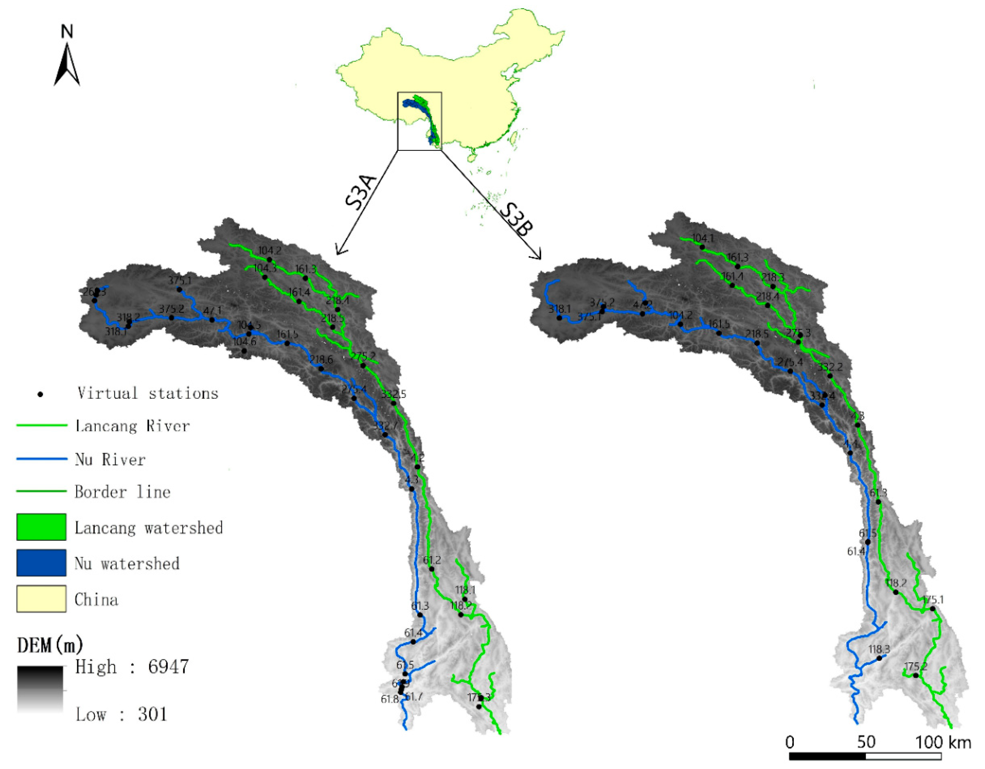
2.1. Study Area
2.2. Data
2.2.1. Sentinel-3 Level-2 Data
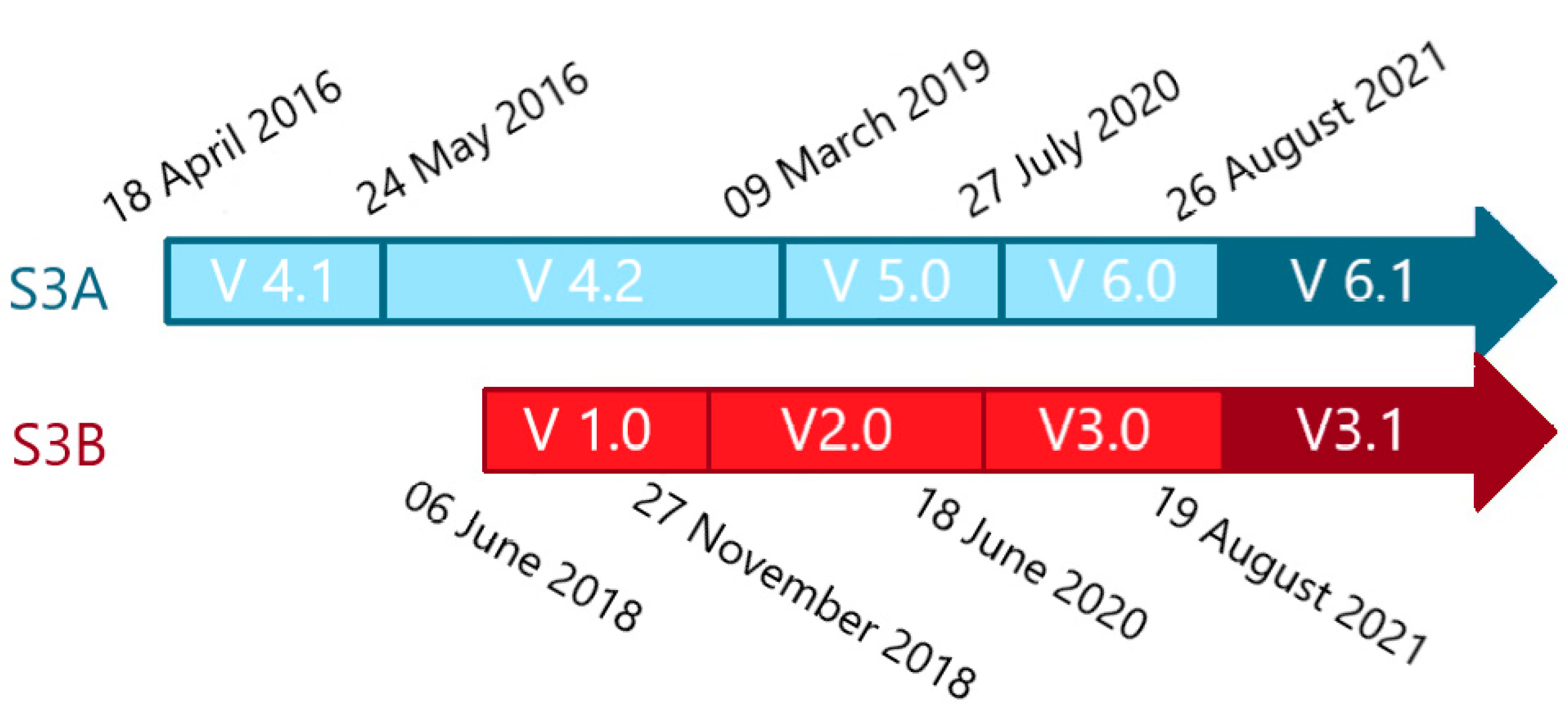
2.2.2. Closed-Loop Tracking Command (CLTC) and Open-Loop Tracking Command (OLTC)
2.2.3. Other Data
3. Methodology
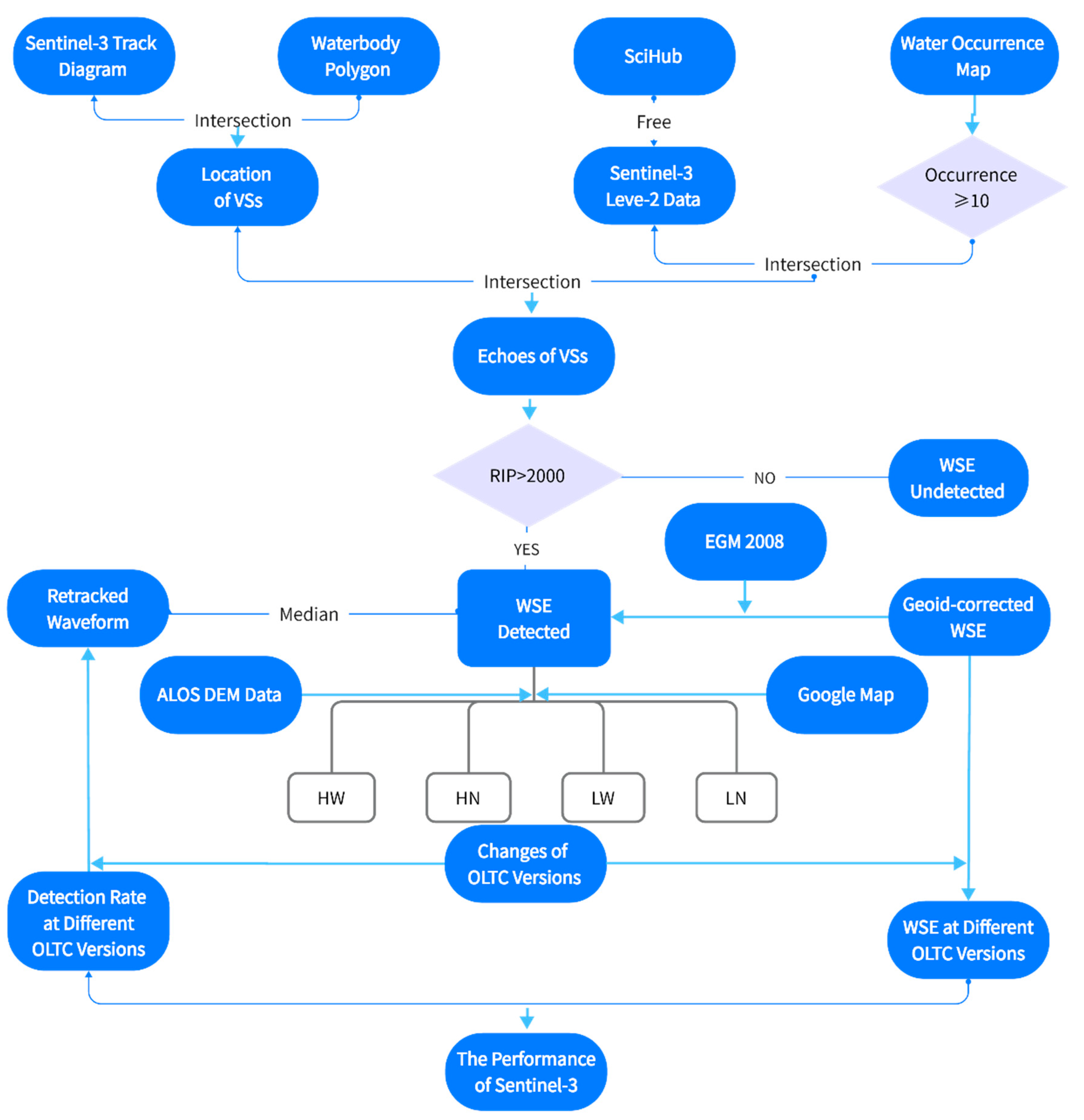
3.1. Methods Overview
3.2. Virtual Stations Extracting
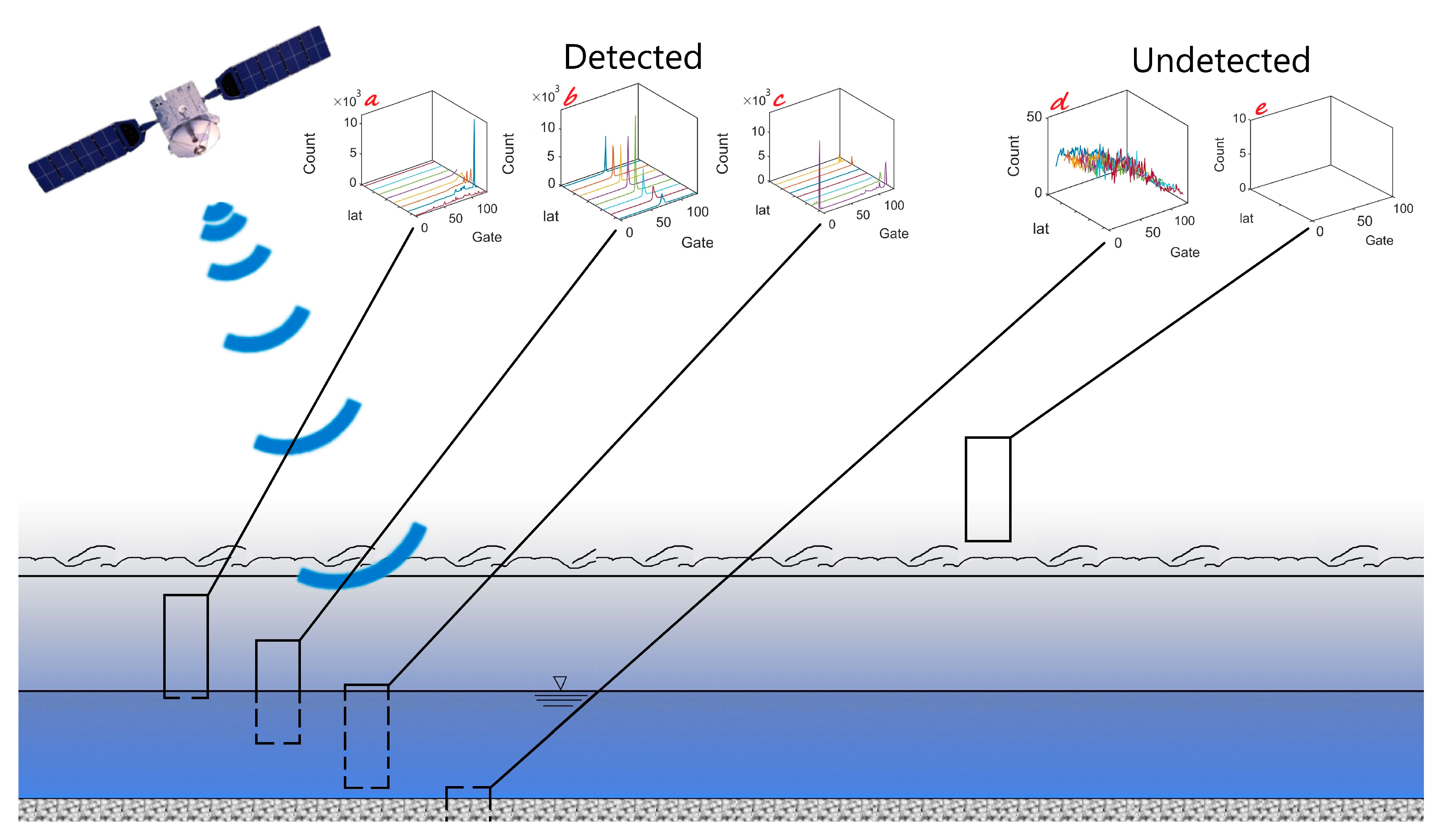
3.3. Water Surface Elevation Detecting
3.4. Elevation and Track Length Partitioning
3.5. Time Series of WSE Constructing
4. Results
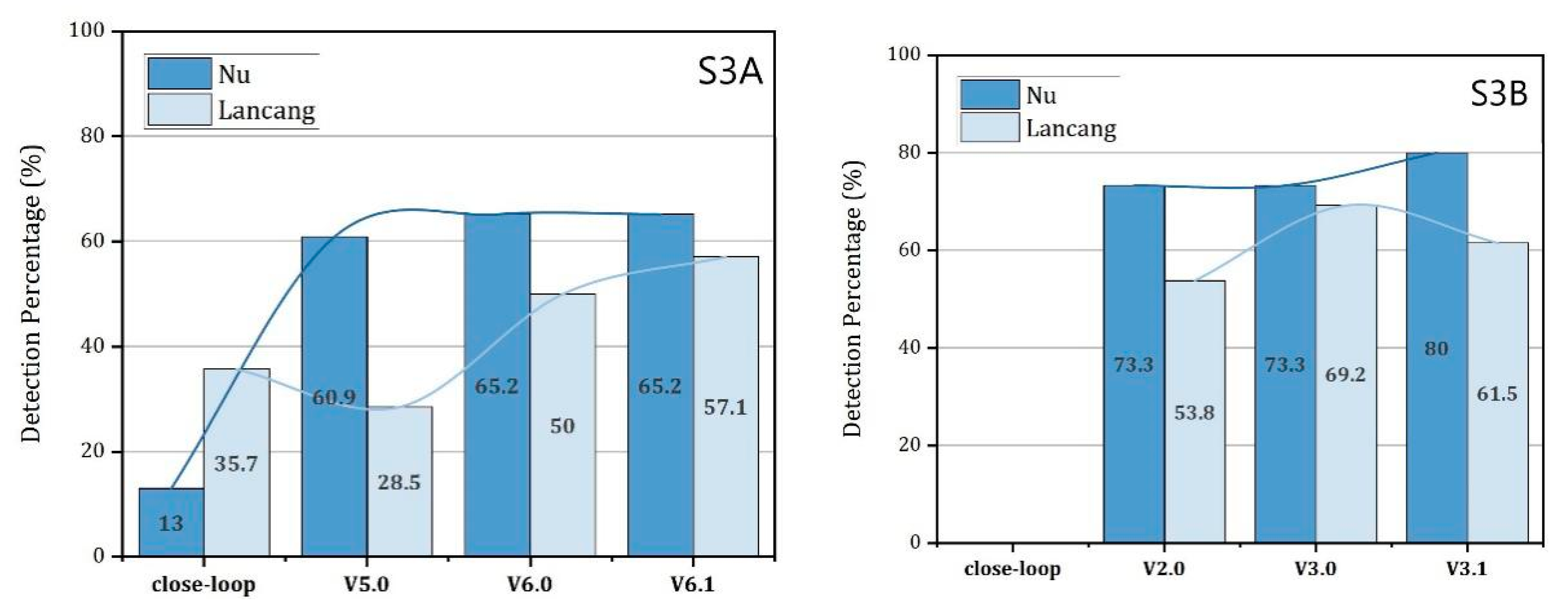
4.1. Performance of S3A and S3B in Closed-Loop Mode and Different OLTC Versions
4.2. Performance of S3A and S3B under Different Track Length and Elevation Conditions
4.3. Performance of S3A and S3B in Lancang and Nu River Basins
5. Discussion
5.1. The Data Quality of S3A and S3B under Various Conditions
5.2. Comparison of S3A and S3B in the Study Region
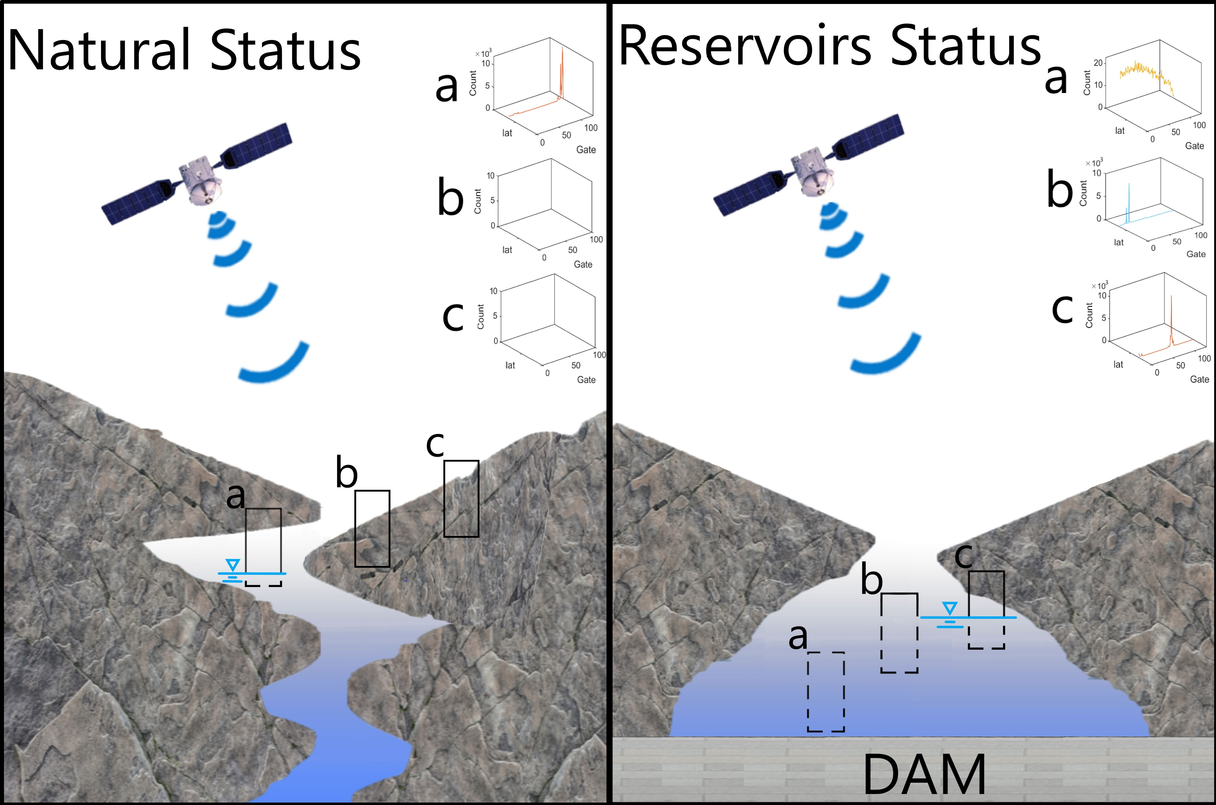
5.3. Impacts of Reservoirs Impoundment on S3A and S3B
5.4. Advantages and Limitations in the Approach and Prospects for Future Research
6. Conclusions
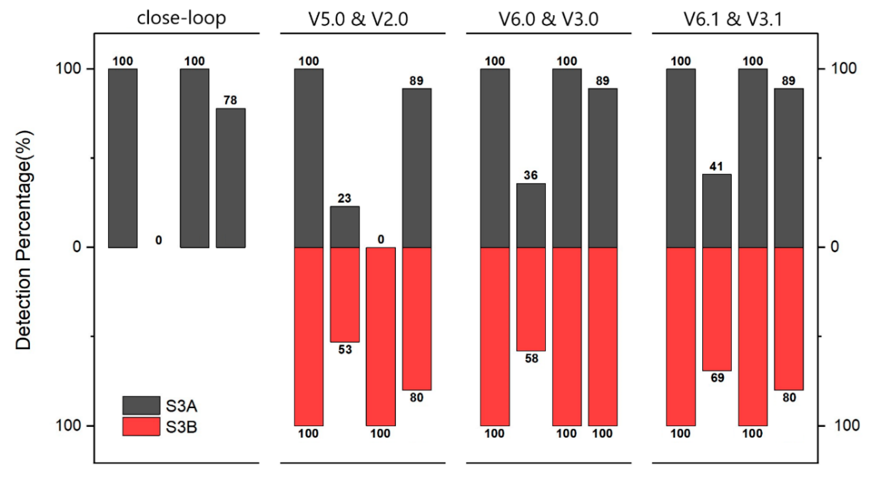
- Transitioning from the closed-loop mode to the open-loop mode and upgrading to newer OLTC versions improved the detection rates for both S3A (from 36.8% in closed-loop to 47.4%, 60.5%, and 63.2% in OLTC V5.0, V6.0, and V6.1, respectively) and S3B (from 64.3% in OLTC V2.0 to 71.4% and 75.0% in OLTC V3.0 and V3.1, respectively) in both the Lancang and Nu River basins.
- The updated OLTC version significantly improved the data quality of VSs in high mountain and narrow rivers, except for a few VSs. Compared to the initial satellite launch, the detection rate improved by 40.9% for S3A and 15.8% for S3B.
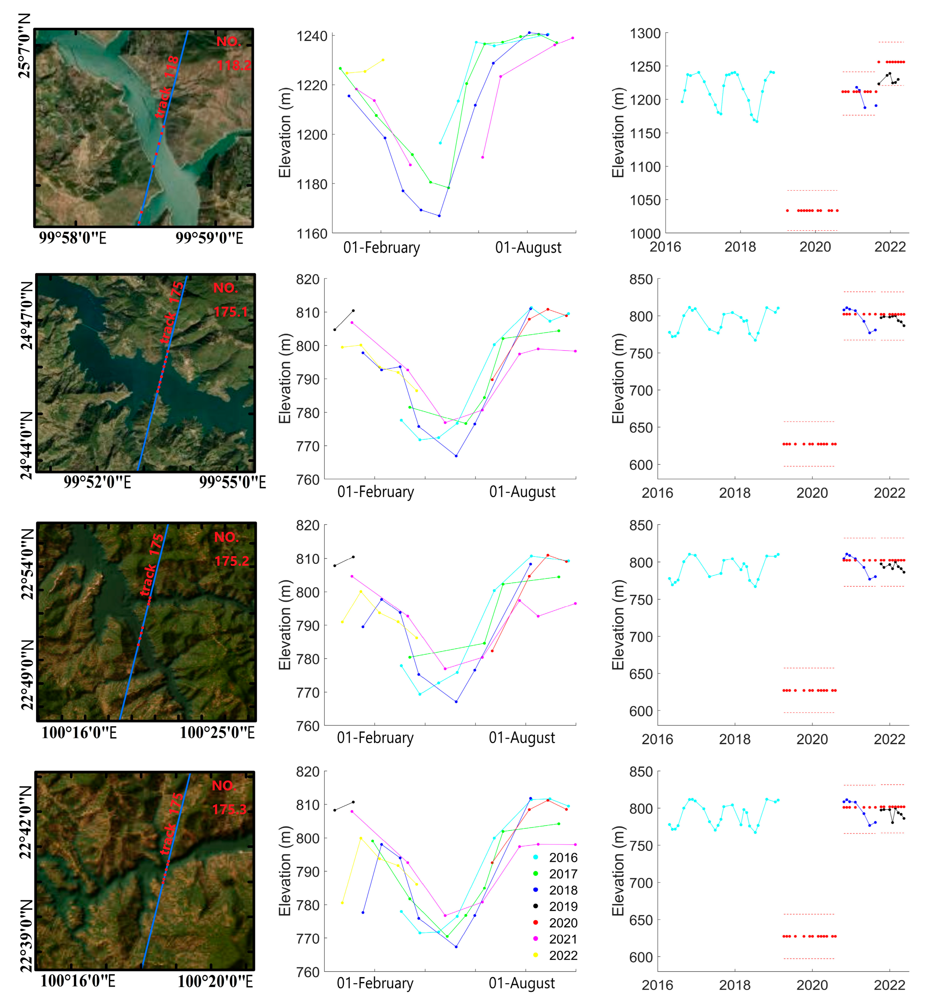
- The closed-loop model of S3A performed better when detecting the WSE in the Lancang River than in the Nu River at lower elevations due to the impoundment of cascade reservoirs, which extended the water surface width of the Lancang River. However, in OLTC V5.0, S3A had difficulty detecting the effective data in the lower reaches of the Lancang River because the elevation of the reservoir water surface resulted in a range window that was too low. This problem has since been addressed by OLTC V6.0 due to the correct placement of the range window.
- In the Lancang River basin, the seasonal variations of the WSE in reservoirs that exceed 60 m may exceed the range window size (60 m), making a complete measurement impossible despite improvements in the OLTC versions.
Author Contributions
Funding
Data Availability Statement
Conflicts of Interest
Appendix A

| Mission | OLTC Version | Date of Activation | Number of VSs | VSs’ Type: Rivers/Lakes/Reservoirs/Glaciers | Update Changes |
|---|---|---|---|---|---|
| Sentinel-3A | V4.1 | 18 April 2016 | 2253 | 2007/246/-/- | - |
| V4.2 | 24 May 2016 | 2253 | 2007/246/-/- | 4 areas of interest between 25°N and 60°N in the open-loop | |
| V5.0 | 9 March 2019 | 33,261 | 17,409/14,427/1,386/39 | 31,008 VSs were added between 60° S and 60°N | |
| V6.0 | 27 July 2020 | 74,050 | 20,100/47,637/4,262/51 | 40,798 VSs were added in the world | |
| V6.1 | 26 August 2021 | 74,050 | 20,100/47,637/4,262/51 | reference elevations of 1262 VSs were improved | |
| Sentinel-3B | V1.0 | 6 June 2018 | 2253 | 2007/246/-/- | - |
| (tandem) | |||||
| V2.0 | 27 November 2018 | 32,515 | 17,016/14,245/1,231/23 | 32515 VSs were added in the 60° S–60°N | |
| V3.0 | 18 June 2020 | 73,629 | 21,719/47,738/4,149/23 | 41,114 VSs were added in the world | |
| V3.1 | 19 August 2021 | 73,629 | 21,719/47,738/4,149/23 | reference elevations of 1153 were improved |
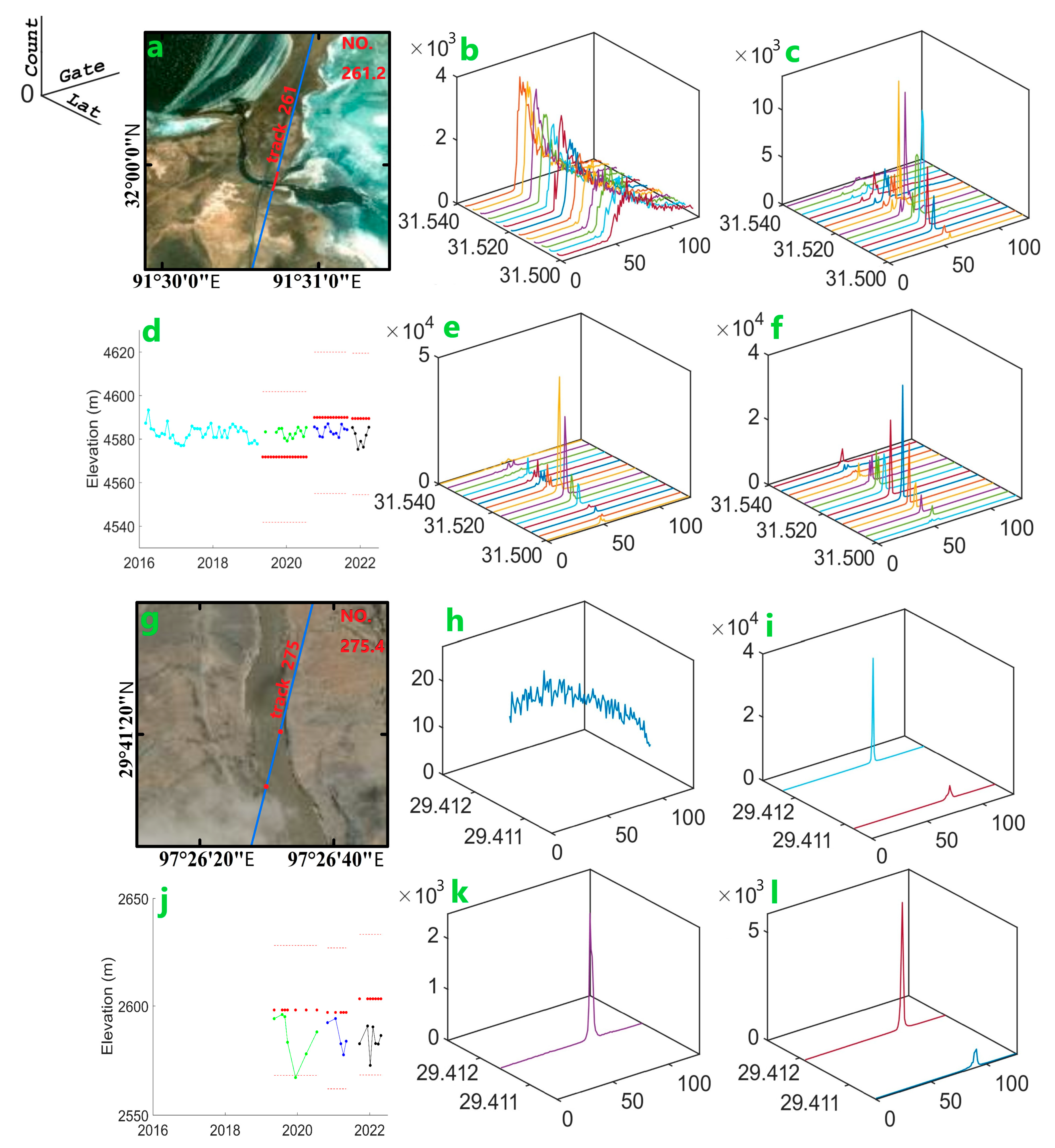
| Station | Detected or Not | Track Length (m) | Elevation (m) | Location | Lon (°) | Lat (°) |
|---|---|---|---|---|---|---|
| 4.3 | Detected | 110 | 1398 | Nu | 98.76 | 27.62 |
| 47.1 | Detected | 80 | 3769 | Nu | 94.20 | 31.48 |
| 61.2 | Detected | 510 | 1304 | Lancang | 99.22 | 25.79 |
| 61.3 | Detected | 270 | 652 | Nu | 98.95 | 24.75 |
| 61.5 | Detected | 280 | 453 | Nu | 98.61 | 23.40 |
| 61.6 | Detected | 340 | 434 | Nu | 98.57 | 23.23 |
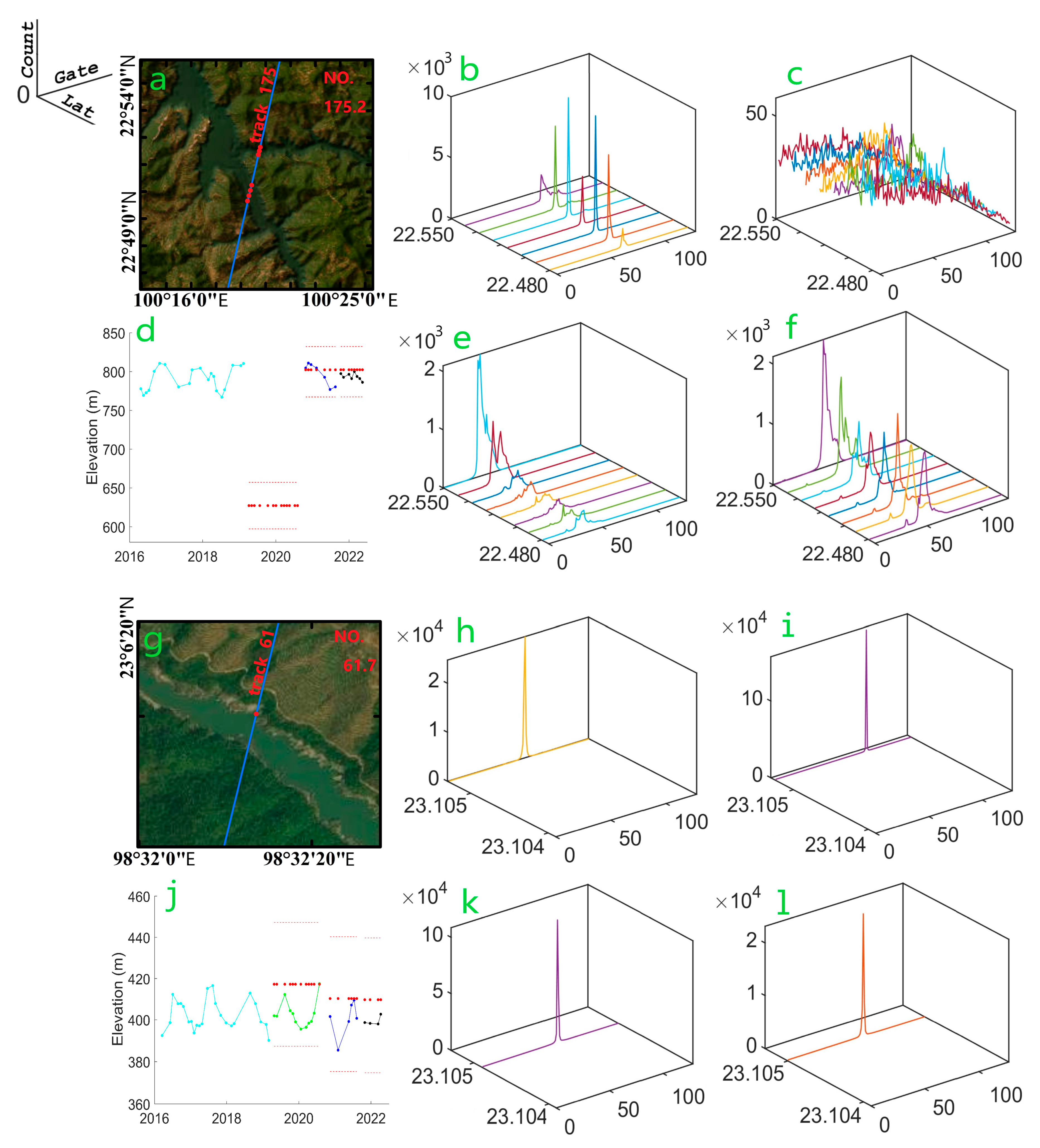
| 61.7 | Detected | 370 | 410 | Nu | 98.54 | 23.11 |
| 61.8 | Detected | 230 | 408 | Nu | 98.52 | 23.05 |
| 61.9 | Detected | 230 | 397 | Nu | 98.51 | 22.98 |
| 104.5 | Detected | 120 | 3452 | Nu | 95.04 | 31.16 |
| 118.1 | Detected | 80 | 1239 | Lancang | 99.98 | 25.11 |
| 118.2 | Detected | 120 | 1272 | Lancang | 99.88 | 24.76 |
| 175.1 | Detected | 1080 | 812 | Lancang | 100.34 | 22.84 |
| 175.2 | Detected | 880 | 769 | Lancang | 100.35 | 22.86 |
| 175.3 | Detected | 840 | 795 | Lancang | 100.30 | 22.66 |
| 261.1 | Detected | 1880 | 4596 | Nu | 91.58 | 32.15 |
| 261.2 | Detected | 1620 | 4597 | Nu | 91.55 | 32.05 |
| 261.3 | Detected | 1540 | 4591 | Nu | 91.51 | 31.92 |
| 275.2 | Detected | 100 | 3022 | Lancang | 97.65 | 30.44 |
| 275.4 | Detected | 190 | 2587 | Nu | 97.44 | 29.69 |
| 318.1 | Detected | 380 | 4405 | Nu | 92.31 | 31.44 |
| 318.2 | Detected | 200 | 4400 | Nu | 92.28 | 31.33 |
| 332.5 | Detected | 150 | 2605 | Lancang | 98.35 | 29.58 |
| 332.7 | Detected | 120 | 2093 | Nu | 98.15 | 28.86 |
| 375.2 | Detected | 190 | 4049 | Nu | 93.27 | 31.53 |
| 4.2 | Undetected | 80 | 1914 | Lancang | 98.89 | 28.13 |
| 61.4 | Undetected | 110 | 559 | Nu | 98.80 | 24.13 |
| 104.2 | Undetected | 110 | 3991 | Lancang | 95.51 | 32.86 |
| 104.3 | Undetected | 150 | 4126 | Lancang | 95.41 | 32.46 |
| 104.4 | Undetected | 40 | 3575 | Nu | 95.08 | 31.31 |
| 104.6 | Undetected | 70 | 4117 | Nu | 94.93 | 30.77 |
| 161.3 | Undetected | 110 | 3707 | Lancang | 96.33 | 32.44 |
| 161.4 | Undetected | 120 | 3713 | Lancang | 96.18 | 31.90 |
| 161.5 | Undetected | 80 | 3226 | Nu | 95.92 | 30.95 |
| 218.4 | Undetected | 80 | 3443 | Lancang | 97.07 | 31.72 |
| 218.5 | Undetected | 120 | 3357 | Lancang | 96.95 | 31.31 |
| 218.6 | Undetected | 120 | 3021 | Nu | 96.69 | 30.37 |
| 375.1 | Undetected | 40 | 4191 | Nu | 93.45 | 32.17 |
| Station | Detected or Not | Track Length (m) | Elevation (m) | Location | Lon (°) | Lat (°) |
|---|---|---|---|---|---|---|
| 4.3 | Detected | 80 | 2230 | Lancang | 98.64 | 28.94 |
| 4.4 | Detected | 290 | 1723 | Nu | 98.47 | 28.31 |
| 47.1 | Detected | 40 | 3914 | Nu | 93.80 | 31.73 |
| 47.2 | Detected | 120 | 3893 | Nu | 93.73 | 31.48 |
| 61.3 | Detected | 60 | 1631 | Lancang | 99.11 | 27.19 |
| 61.4 | Detected | 340 | 950 | Nu | 98.88 | 26.28 |
| 61.5 | Detected | 150 | 924 | Nu | 98.87 | 26.27 |
| 104.1 | Detected | 40 | 4160 | Lancang | 95.09 | 33.00 |
| 104.2 | Detected | 80 | 3591 | Nu | 94.60 | 31.24 |
| 118.2 | Detected | 1200 | 1228 | Lancang | 99.51 | 25.12 |
| 118.3 | Detected | 350 | 495 | Nu | 99.13 | 23.62 |
| 161.3 | Detected | 40 | 3835 | Lancang | 95.90 | 32.56 |
| 161.4 | Detected | 80 | 3913 | Lancang | 95.78 | 32.13 |
| 161.5 | Detected | 110 | 3363 | Nu | 95.47 | 31.04 |
| 175.1 | Detected | 1280 | 989 | Lancang | 100.35 | 24.75 |
| 175.2 | Detected | 1350 | 807 | Lancang | 99.97 | 23.23 |
| 218.3 | Detected | 80 | 3580 | Lancang | 96.71 | 32.11 |
| 218.4 | Detected | 80 | 3541 | Lancang | 96.59 | 31.67 |
| 218.5 | Detected | 190 | 3125 | Nu | 96.35 | 30.81 |
| 275.3 | Detected | 120 | 3316 | Lancang | 97.29 | 30.83 |
| 275.4 | Detected | 110 | 2734 | Nu | 97.11 | 30.17 |
| 332.2 | Detected | 110 | 2834 | Lancang | 98.01 | 30.06 |
| 375.1 | Detected | 80 | 4173 | Nu | 92.84 | 31.64 |
| 375.2 | Detected | 40 | 4189 | Nu | 92.81 | 31.53 |
| 275.2 | Undetected | 110 | 3165 | Lancang | 97.33 | 30.99 |
| 318.1 | Undetected | 120 | 4498 | Nu | 91.83 | 31.39 |
| 332.3 | Undetected | 50 | 3765 | Nu | 97.89 | 29.62 |
| 332.4 | Undetected | 50 | 2392 | Nu | 97.83 | 29.40 |
| S3A | S3B | |||||||
|---|---|---|---|---|---|---|---|---|
| Closed-Loop | V5.0 | V6.0 | V6.1 | V2.0 | V3.0 | V3.1 | ||
| 4.3 | √ | √ | √ | 4.3 | √ | √ | √ | |
| 47.1 | √ | √ | √ | 4.4 | √ | √ | √ | |
| 61.2 | √ | √ | √ | 47.1 | √ | √ | ||
| 61.3 | √ | √ | √ | 47.2 | √ | √ | √ | |
| 61.5 | √ | √ | √ | 61.3 | √ | |||
| 61.6 | √ | √ | √ | 61.4 | √ | √ | √ | |
| 61.7 | √ | √ | 61.5 | √ | √ | √ | ||
| 61.8 | √ | √ | √ | 104.1 | √ | √ | ||
| 61.9 | √ | √ | √ | 104.2 | √ | √ | √ | |
| 104.5 | √ | √ | √ | 118.2 | √ | √ | √ | |
| 118.1 | √ | √ | √ | 118.3 | √ | √ | √ | |
| 118.2 | √ | √ | √ | 161.3 | √ | |||
| 175.1 | √ | √ | √ | 161.4 | √ | √ | √ | |
| 175.2 | √ | √ | √ | 161.5 | √ | √ | √ | |
| 175.3 | √ | √ | √ | 175.1 | √ | √ | √ | |
| 261.1 | √ | √ | √ | √ | 175.2 | √ | √ | √ |
| 261.2 | √ | √ | √ | √ | 218.3 | √ | √ | √ |
| 261.3 | √ | √ | √ | √ | 218.4 | √ | √ | √ |
| 275.2 | √ | √ | √ | 218.5 | √ | √ | √ | |
| 275.4 | √ | √ | √ | 275.3 | √ | |||
| 318.1 | √ | √ | 275.4 | √ | √ | |||
| 318.2 | √ | √ | 332.2 | √ | ||||
| 332.5 | √ | √ | √ | 375.1 | √ | |||
| 332.7 | √ | √ | √ | 375.2 | √ | √ | √ | |
| 375.2 | √ | √ | √ | |||||
References
- Kleinherenbrink, M.; Lindenbergh, R.C.; Ditmar, P.G. Monitoring of lake level changes on the Tibetan Plateau and Tian Shan by retracking Cryosat SARIn waveforms. J. Hydrol. 2015, 521, 119–131. [Google Scholar] [CrossRef]
- Nielsen, K.; Stenseng, L.; Andersen, O.B.; Villadsen, H.; Knudsen, P. Validation of CryoSat-2 SAR mode based lake levels. Remote Sens. Environ. 2015, 171, 162–170. [Google Scholar] [CrossRef] [Green Version]
- Chen, T.; Song, C.; Zhan, P.; Fan, C. Densifying and Optimizing the Water Level Series for Large Lakes from Multi-Orbit ICESat-2 Observations. Remote Sens. 2023, 15, 780. [Google Scholar] [CrossRef]
- Tian, B.; Gao, P.; Mu, X.; Zhao, G. Water Area Variation and River–Lake Interactions in the Poyang Lake from 1977–2021. Remote Sens. 2023, 15, 600. [Google Scholar] [CrossRef]
- Kandekar, V.U.; Pande, C.B.; Rajesh, J.; Atre, A.A.; Gorantiwar, S.D.; Kadam, S.A.; Gavit, B. Surface water dynamics analysis based on sentinel imagery and Google Earth Engine Platform: A case study of Jayakwadi dam. Sustain. Water Resour. Manag. 2021, 7, 44. [Google Scholar] [CrossRef]
- Domeneghetti, A.; Tarpanelli, A.; Brocca, L.; Barbetta, S.; Moramarco, T.; Castellarin, A.; Brath, A. The use of remote sensing-derived water surface data for hydraulic model calibration. Remote Sens. Environ. 2014, 149, 130–141. [Google Scholar] [CrossRef]
- Ahmed, R.; Rawat, M.; Wani, G.F.; Ahmad, S.T.; Ahmed, P.; Jain, S.K.; Meraj, G.; Mir, R.A.; Rather, A.F.; Farooq, M. Glacial Lake Outburst Flood Hazard and Risk Assessment of Gangabal Lake in the Upper Jhelum Basin of Kashmir Himalaya Using Geospatial Technology and Hydrodynamic Modeling. Remote Sens. 2022, 14, 5957. [Google Scholar] [CrossRef]
- Yin, Z.; Li, X.; Huang, C.; Chen, W.; Hou, B.; Li, X.; Han, W.; Hou, P.; Han, J.; Ren, C.; et al. Analysis of the Formation Mechanism of Medium and Low-Temperature Geothermal Water in Wuhan Based on Hydrochemical Characteristics. Water 2023, 15, 227. [Google Scholar] [CrossRef]
- Hu, W.-F.; Yao, J.-Q.; He, Q.; Yang, Q. Spatial and temporal variability of water vapor content during 1961–2011 in Tianshan Mountains, China. J. Mt. Sci. 2015, 12, 571–581. [Google Scholar] [CrossRef]
- Wongchuig-Correa, S.; de Paiva, R.C.D.; Biancamaria, S.; Collischonn, W. Assimilation of future SWOT-based river elevations, surface extent observations and discharge estimations into uncertain global hydrological models. J. Hydrol. 2020, 590, 125473. [Google Scholar] [CrossRef]
- Jiang, L.; Nielsen, K.; Andersen, O.B.; Bauer-Gottwein, P. Monitoring recent lake level variations on the Tibetan Plateau using CryoSat-2 SARIn mode data. J. Hydrol. 2017, 544, 109–124. [Google Scholar] [CrossRef] [Green Version]
- Kittel, C.M.M.; Jiang, L.; Tøttrup, C.; Bauer-Gottwein, P. Sentinel-3 radar altimetry for river monitoring—A catchment-scale evaluation of satellite water surface elevation from Sentinel-3A and Sentinel-3B. Hydrol. Earth Syst. Sci. 2021, 25, 333–357. [Google Scholar] [CrossRef]
- Sichangi, A.W.; Wang, L.; Yang, K.; Chen, D.; Wang, Z.; Li, X.; Zhou, J.; Liu, W.; Kuria, D.; Naturvetenskapliga, F.; et al. Estimating continental river basin discharges using multiple remote sensing data sets. Remote Sens. Environ. 2016, 179, 36–53. [Google Scholar] [CrossRef] [Green Version]
- Zhang, X.; Jiang, L.; Liu, Z.; Kittel, C.M.; Yao, Z.; Druce, D.; Wang, R.; Tøttrup, C.; Liu, J.; Jiang, H.; et al. Flow regime changes in the Lancang River, revealed by integrated modeling with multiple Earth observation datasets. Sci. Total. Environ. 2023, 862, 160656. [Google Scholar] [CrossRef]
- Lobera, G.; Besné, P.; Vericat, D.; López-Tarazón, J.; Tena, A.; Aristi, I.; Díez, J.; Ibisate, A.; Larrañaga, A.; Elosegi, A.; et al. Geomorphic status of regulated rivers in the Iberian Peninsula. Sci. Total. Environ. 2015, 508, 101–114. [Google Scholar] [CrossRef]
- Blöschl, G. Three hypotheses on changing river flood hazards. Hydrol. Earth Syst. Sci. 2022, 26, 5015–5033. [Google Scholar] [CrossRef]
- Debnath, J.; Sahariah, D.; Lahon, D.; Nath, N.; Chand, K.; Meraj, G.; Farooq, M.; Kumar, P.; Kanga, S.; Singh, S.K. Geospatial modeling to assess the past and future land use-land cover changes in the Brahmaputra Valley, NE India, for sustainable land resource management. Environ. Sci. Pollut. Res. 2022; ahead of print. [Google Scholar] [CrossRef]
- Hardeng, J.; Bakke, J.; Sabatier, P.; Støren, E.W.N.; Van der Bilt, W. Lake sediments from southern Norway capture Holocene variations in flood seasonality. Quat. Sci. Rev. 2022, 290, 107643. [Google Scholar] [CrossRef]
- Hannah, D.M.; DeMuth, S.; van Lanen, H.A.J.; Looser, U.; Prudhomme, C.; Rees, G.; Stahl, K.; Tallaksen, L.M. Large-scale river flow archives: Importance, current status and future needs. Hydrol. Process. 2011, 25, 1191–1200. [Google Scholar] [CrossRef]
- Schneider, C.; Flörke, M.; De Stefano, L.; Petersen-Perlman, J.D. Hydrological threats to riparian wetlands of international importance—A global quantitative and qualitative analysis. Hydrol. Earth Syst. Sci. 2017, 21, 2799–2815. [Google Scholar] [CrossRef] [Green Version]
- Thu, H.N.; Wehn, U. Data sharing in international transboundary contexts: The Vietnamese perspective on data sharing in the Lower Mekong Basin. J. Hydrol. 2016, 536, 351–364. [Google Scholar] [CrossRef] [Green Version]
- Hiep, N.H.; Luong, N.D.; Ni, C.-F.; Hieu, B.T.; Huong, N.L.; Du Duong, B. Factors influencing the spatial and temporal variations of surface runoff coefficient in the Red River basin of Vietnam. Environ. Earth Sci. 2023, 82, 56. [Google Scholar] [CrossRef]
- Li, Y.; Li, B.; Yuan, Y.; Lei, Q.; Jiang, Y.; Liu, Y.; Li, R.; Liu, W.; Zhai, D.; Xu, J. Trends in total nitrogen concentrations in the Three Rivers Headwater Region. Sci. Total. Environ. 2022, 852, 158462. [Google Scholar] [CrossRef]
- Zhong, R.; Zhao, T.; Chen, X.; Jin, H. Monitoring drought in ungauged areas using satellite altimetry: The Standardized River Stage Index. J. Hydrol. 2022, 612, 128308. [Google Scholar] [CrossRef]
- Jiang, L.; Nielsen, K.; Dinardo, S.; Andersen, O.B.; Bauer-Gottwein, P. Evaluation of Sentinel-3 SRAL SAR altimetry over Chinese rivers. Remote Sens. Environ. 2020, 237, 111546. [Google Scholar] [CrossRef]
- Zhang, X.; Jiang, L.; Kittel, C.M.M.; Yao, Z.; Nielsen, K.; Liu, Z.; Wang, R.; Liu, J.; Andersen, O.B.; Bauer-Gottwein, P. On the Performance of Sentinel-3 Altimetry Over New Reservoirs: Approaches to Determine Onboard A Priori Elevation. Geophys. Res. Lett. 2020, 47, e2020GL088770. [Google Scholar] [CrossRef]
- Arsen, A.; Crétaux, J.-F.; Del Rio, R.A. Use of SARAL/AltiKa over Mountainous Lakes, Intercomparison with Envisat Mission. Mar. Geodesy 2015, 38, 534–548. [Google Scholar] [CrossRef]
- Biancamaria, S.; Frappart, F.; Leleu, A.-S.; Marieu, V.; Blumstein, D.; Desjonquères, J.-D.; Boy, F.; Sottolichio, A.; Valle-Levinson, A. Satellite radar altimetry water elevations performance over a 200 m wide river: Evaluation over the Garonne River. Adv. Space Res. 2017, 59, 128–146. [Google Scholar] [CrossRef] [Green Version]
- Jiang, M.; Behrens, P.; Wang, T.; Zhipeng, T.; Yu, Y.; Chen, D.; Liu, L.; Ren, Z.; Zhou, W.; Zhu, S.; et al. Provincial and sector-level material footprints in China. Proc. Natl. Acad. Sci. USA 2019, 116, 26484–26490. [Google Scholar] [CrossRef] [PubMed] [Green Version]
- Boergens, E.; Nielsen, K.; Andersen, O.B.; Dettmering, D.; Seitz, F. River Levels Derived with CryoSat-2 SAR Data Classification—A Case Study in the Mekong River Basin. Remote Sens. 2017, 9, 1238. [Google Scholar] [CrossRef] [Green Version]
- Chelton, D.B.; Esbensen, S.K.; Schlax, M.G.; Thum, N.; Freilich, M.H.; Wentz, F.J.; Gentemann, C.L.; McPhaden, M.J.; Schopf, P.S. Observations of coupling between surface wind stress and sea surface temperature in the eastern tropical Pacific. J. Clim. 2001, 14, 1479–1498. [Google Scholar] [CrossRef]
- Chelton, D.B.; Freilich, M.H.; Johnson, J.R. Evaluation of Unambiguous Vector Winds from the Seasat Scatterometer. J. Atmos. Ocean. Technol. 1989, 6, 1024–1039. [Google Scholar] [CrossRef]
- Wingham, D.; Francis, C.; Baker, S.; Bouzinac, C.; Brockley, D.; Cullen, R.; de Chateau-Thierry, P.; Laxon, S.; Mallow, U.; Mavrocordatos, C.; et al. CryoSat: A mission to determine the fluctuations in Earth’s land and marine ice fields. Nat. Hazards Oceanogr. Process. Satell. Data 2006, 37, 841–871. [Google Scholar] [CrossRef]
- Frappart, F.; Legrésy, B.; Niño, F.; Blarel, F.; Fuller, N.; Fleury, S.; Birol, F.; Calmant, S. An ERS-2 altimetry reprocessing compatible with ENVISAT for long-term land and ice sheets studies. Remote Sens. Environ. 2016, 184, 558–581. [Google Scholar] [CrossRef]
- Berry, P.A.M.; Garlick, J.D.; Freeman, J.A.; Mathers, E.L. Global inland water monitoring from multi-mission altimetry. Geophys. Res. Lett. 2005, 32, 22814. [Google Scholar] [CrossRef]
- Normandin, C.; Frappart, F.; Diepkilé, A.T.; Marieu, V.; Mougin, E.; Blarel, F.; Lubac, B.; Braquet, N.; Ba, A. Evolution of the Performances of Radar Altimetry Missions from ERS-2 to Sentinel-3A over the Inner Niger Delta. Remote Sens. 2018, 10, 833. [Google Scholar] [CrossRef] [Green Version]
- Dawson, G.; Landy, J.; Tsamados, M.; Komarov, A.S.; Howell, S.; Heorton, H.; Krumpen, T. A 10-year record of Arctic summer sea ice freeboard from CryoSat-2. Remote Sens. Environ. 2022, 268, 112744. [Google Scholar] [CrossRef]
- Morris, A.; Moholdt, G.; Gray, L.; Schuler, T.V.; Eiken, T. CryoSat-2 interferometric mode calibration and validation: A case study from the Austfonna ice cap, Svalbard. Remote Sens. Environ. 2021, 269, 112805. [Google Scholar] [CrossRef]
- Nilsson, B.; Andersen, O.B.; Ranndal, H.; Rasmussen, M.L. Consolidating ICESat-2 Ocean Wave Characteristics with CryoSat-2 during the CRYO2ICE Campaign. Remote Sens. 2022, 14, 1300. [Google Scholar] [CrossRef]
- Chen, P.; An, Z.; Xue, H.; Yao, Y.; Yang, X.; Wang, R.; Wang, Z. INPPTR: An improved retracking algorithm for inland water levels estimation using Cryosat-2 SARin data. J. Hydrol. 2022, 613, 128439. [Google Scholar] [CrossRef]
- Kleinherenbrink, M.; Naeije, M.; Slobbe, C.; Egido, A.; Smith, W. The performance of CryoSat-2 fully-focussed SAR for inland water-level estimation. Remote Sens. Environ. 2020, 237, 111589. [Google Scholar] [CrossRef]
- Li, P.; Li, H.; Chen, F.; Cai, X. Monitoring Long-Term Lake Level Variations in Middle and Lower Yangtze Basin over 2002–2017 through Integration of Multiple Satellite Altimetry Datasets. Remote Sens. 2020, 12, 1448. [Google Scholar] [CrossRef]
- Heorton, H.; Tsamados, M.; Armitage, T.; Ridout, A.; Landy, J. CryoSat-2 Significant Wave Height in Polar Oceans Derived Using a Semi-Analytical Model of Synthetic Aperture Radar 2011–2019. Remote Sens. 2021, 13, 4166. [Google Scholar] [CrossRef]
- Lian, T.; Xin, X.; Peng, Z.; Li, F.; Zhang, H.; Yu, S.; Liu, H. Estimating Evapotranspiration over Heterogeneous Surface with Sentinel-2 and Sentinel-3 Data: A Case Study in Heihe River Basin. Remote Sens. 2022, 14, 1349. [Google Scholar] [CrossRef]
- Shen, M.; Duan, H.; Cao, Z.; Xue, K.; Qi, T.; Ma, J.; Liu, D.; Song, K.; Huang, C.; Song, X. Sentinel-3 OLCI observations of water clarity in large lakes in eastern China: Implications for SDG 6.3.2 evaluation. Remote Sens. Environ. 2020, 247, 111950. [Google Scholar] [CrossRef]
- Taburet, N.; Zawadzki, L.; Vayre, M.; Blumstein, D.; Le Gac, S.; Boy, F.; Raynal, M.; Labroue, S.; Crétaux, J.-F.; Femenias, P. S3MPC: Improvement on Inland Water Tracking and Water Level Monitoring from the OLTC Onboard Sentinel-3 Altimeters. Remote Sens. 2020, 12, 3055. [Google Scholar] [CrossRef]
- Wan, Y.; Zhang, R.; Pan, X.; Fan, C.; Dai, Y. Evaluation of the Significant Wave Height Data Quality for the Sentinel-3 Synthetic Aperture Radar Altimeter. Remote Sens. 2020, 12, 3107. [Google Scholar] [CrossRef]
- Vu, D.T.; Dang, T.D.; Galelli, S.; Hossain, F. Satellite observations reveal 13 years of reservoir filling strategies, operating rules, and hydrological alterations in the Upper Mekong River basin. Hydrol. Earth Syst. Sci. 2022, 26, 2345–2364. [Google Scholar] [CrossRef]
- Zhang, C.; Lv, A.; Zhu, W.; Yao, G.; Qi, S. Using Multisource Satellite Data to Investigate Lake Area, Water Level, and Water Storage Changes of Terminal Lakes in Ungauged Regions. Remote Sens. 2021, 13, 3221. [Google Scholar] [CrossRef]
- Biancamaria, S.; Schaedele, T.; Blumstein, D.; Frappart, F.; Boy, F.; Desjonquères, J.-D.; Pottier, C.; Blarel, F.; Niño, F. Validation of Jason-3 tracking modes over French rivers. Remote Sens. Environ. 2018, 209, 77–89. [Google Scholar] [CrossRef] [Green Version]
- Martin-Puig, C.; Leuliette, E.; Lillibridge, J.; Roca, M. Evaluating the Performance of Jason-2 Open-Loop and Closed-Loop Tracker Modes. J. Atmos. Ocean. Technol. 2016, 33, 2277–2288. [Google Scholar] [CrossRef]
- Yuan, J.; Guo, J.; Niu, Y.; Zhu, C.; Li, Z.; Liu, X. Denoising Effect of Jason-1 Altimeter Waveforms with Singular Spectrum Analysis: A Case Study of Modelling Mean Sea Surface Height over South China Sea. J. Mar. Sci. Eng. 2020, 8, 426. [Google Scholar] [CrossRef]
- Abdalla, S. Are Jason-2 significant wave height measurements still useful. Adv. Space Res. 2021, 68, 802–807. [Google Scholar] [CrossRef]
- Vignudelli, S.; Cipollini, P.; Gommenginger, C.; Gleason, S.; Snaith, H.M.; Coelho, H.; Fernandes, M.J.; Lázaro, C.; Nunes, A.L.; Gómez-Enri, J.; et al. Satellite Altimetry: Sailing Closer to the Coast. Remote Sens. Chang. Ocean. 2011, 217–238. [Google Scholar] [CrossRef]
- Steunou, N.; Picot, N.; Sengenes, P.; Noubel, J.; Frery, M. AltiKa Radiometer: Instrument Description and In–Flight Performance. Mar. Geodesy 2015, 38, 43–61. [Google Scholar] [CrossRef]
- Le Gac, S.; Boy, F.; Blumstein, D.; Lasson, L.; Picot, N. Benefits of the Open-Loop Tracking Command (OLTC): Extending conventional nadir altimetry to inland waters monitoring. Adv. Space Res. 2021, 68, 843–852. [Google Scholar] [CrossRef]
- Yang, Y.; Weng, B.; Yan, D.; Niu, Y.; Dai, Y.; Li, M.; Gong, X. Partitioning the contributions of cryospheric change to the increase of streamflow on the Nu River. J. Hydrol. 2021, 598, 126330. [Google Scholar] [CrossRef]
- Zhong, X.; Li, J.; Wang, J.; Zhang, J.; Liu, L.; Ma, J. Linear and Nonlinear Characteristics of Long-Term NDVI Using Trend Analysis: A Case Study of Lancang-Mekong River Basin. Remote Sens. 2022, 14, 6271. [Google Scholar] [CrossRef]
- Jiang, J.; Zhu, S.; Wang, W.; Li, Y.; Li, N. Coupling coordination between new urbanisation and carbon emissions in China. Sci. Total. Environ. 2022, 850, 158076. [Google Scholar] [CrossRef]
- Tian, F.; Hou, S.; Morovati, K.; Zhang, K.; Nan, Y.; Lu, X.X.; Ni, G. Exploring spatio-temporal patterns of sediment load and driving factors in Lancang-Mekong River basin before operation of mega-dams (1968–2002). J. Hydrol. 2023, 617, 128922. [Google Scholar] [CrossRef]
- Xu, X.; Zhang, X.; Li, X.; Henry, A.J. Evaluation of the Applicability of Three Methods for Climatic Spatial Interpolation in the Hengduan Mountains Region. J. Hydrometeorol. 2023, 24, 35–51. [Google Scholar] [CrossRef]
- Yuan, X.; Wang, J.; He, D.; Lu, Y.; Sun, J.; Li, Y.; Guo, Z.; Zhang, K.; Li, F. Influence of cascade reservoir operation in the Upper Mekong River on the general hydrological regime: A combined data-driven modeling approach. J. Environ. Manag. 2022, 324, 116339. [Google Scholar] [CrossRef] [PubMed]
- Sun, Z.; Sun, L.; Zheng, H.; Li, Z. Estimation of sedimentation in the Manwan and Jinghong reservoirs on the Lancang river. Water Supply 2022, 22, 4307–4319. [Google Scholar] [CrossRef]
- Lizundia-Loiola, J.; Franquesa, M.; Khairoun, A.; Chuvieco, E. Global burned area mapping from Sentinel-3 Synergy and VIIRS active fires. Remote Sens. Environ. 2022, 282, 113298. [Google Scholar] [CrossRef]
- Windle, A.E.; Evers-King, H.; Loveday, B.R.; Ondrusek, M.; Silsbe, G.M. Evaluating Atmospheric Correction Algorithms Applied to OLCI Sentinel-3 Data of Chesapeake Bay Waters. Remote Sens. 2022, 14, 1881. [Google Scholar] [CrossRef]
- Desjonquères, J.D.; Carayon, G.; Steunou, N.; Lambin, J. Poseidon-3 Radar Altimeter: New Modes and In-Flight Performances. Mar. Geodesy 2010, 33, 53–79. [Google Scholar] [CrossRef]
- Pekel, J.-F.; Cottam, A.; Gorelick, N.; Belward, A.S. High-resolution mapping of global surface water and its long-term changes. Nature 2016, 540, 418–422. [Google Scholar] [CrossRef]
- Michailovsky, C.I.; McEnnis, S.; Berry, P.A.M.; Smith, R.; Bauer-Gottwein, P. River monitoring from satellite radar altimetry in the Zambezi River basin. Hydrol. Earth Syst. Sci. 2012, 16, 2181–2192. [Google Scholar] [CrossRef] [Green Version]
- Wang, J.; Tang, Q.; Yun, X.; Chen, A.; Sun, S.; Yamazaki, D. Flood inundation in the Lancang-Mekong River Basin: Assessing the role of summer monsoon. J. Hydrol. 2022, 612, 128075. [Google Scholar] [CrossRef]
- Jiang, L.; Nielsen, K.; Andersen, O.B.; Bauer-Gottwein, P. CryoSat-2 radar altimetry for monitoring freshwater resources of China. Remote Sens. Environ. 2017, 200, 125–139. [Google Scholar] [CrossRef] [Green Version]


| S3A | S3B | |||||||
|---|---|---|---|---|---|---|---|---|
| Total | 25/38 (65.8%) | 23/28 (82.1%) | ||||||
| Stable | Unstable | Stable | Unstable | |||||
| Total | 3/38 (7.9%) | 22/38 (57.9%) | 13/28 (46.4%) | 10/28 (41.7%) | ||||
| closed-loop | V5.0 | V6.0 | V6.1 | V1.0 | V2.0 | V3.0 | V3.1 | |
| Total | 14/38 (36.8%) | 18/38 (47.4%) | 23/38 (60.5%) | 24/38 (63.2%) | - | 18/28 (64.3%) | 20/28 (71.4%) | 21/28 (75.0%) |
| HW | 3/3 (100.0%) | 3/3 (100.0%) | 3/3 (100.0%) | 3/3 (100.0%) | - | 1/1 (100.0%) | 1/1 (100.0%) | 1/1 (100.0%) |
| HN | 0/22 (0%) | 7/22 (31.8%) | 8/22 (36.4%) | 9/22 (40.9%) | - | 10/19 (52.6%) | 11/19 (57.9%) | 13/19 (68.4%) |
| LW | 4/4 (100.0%) | 0/4 (0.0%) | 4/4 (100.0%) | 4/4 (100.0%) | - | 3/3 (100.0%) | 3/3 (100.0%) | 3/3 (100.0%) |
| LN | 7/9 (77.8%) | 8/9 (88.8%) | 8/9 (88.8%) | 8/9 (88.8%) | - | 4/5 (80.0%) | 5/5 (100.0%) | 4/5 (80.0%) |
Disclaimer/Publisher’s Note: The statements, opinions and data contained in all publications are solely those of the individual author(s) and contributor(s) and not of MDPI and/or the editor(s). MDPI and/or the editor(s) disclaim responsibility for any injury to people or property resulting from any ideas, methods, instructions or products referred to in the content. |
© 2023 by the authors. Licensee MDPI, Basel, Switzerland. This article is an open access article distributed under the terms and conditions of the Creative Commons Attribution (CC BY) license (https://creativecommons.org/licenses/by/4.0/).
Share and Cite
Cheng, Y.; Zhang, X.; Yao, Z. On the Performance of Sentinel-3 Altimetry over High Mountain and Cascade Reservoirs Basins: Case of the Lancang and Nu River Basins. Remote Sens. 2023, 15, 1769. https://doi.org/10.3390/rs15071769
Cheng Y, Zhang X, Yao Z. On the Performance of Sentinel-3 Altimetry over High Mountain and Cascade Reservoirs Basins: Case of the Lancang and Nu River Basins. Remote Sensing. 2023; 15(7):1769. https://doi.org/10.3390/rs15071769
Chicago/Turabian StyleCheng, Yu, Xingxing Zhang, and Zhijun Yao. 2023. "On the Performance of Sentinel-3 Altimetry over High Mountain and Cascade Reservoirs Basins: Case of the Lancang and Nu River Basins" Remote Sensing 15, no. 7: 1769. https://doi.org/10.3390/rs15071769