Article

Generation of Multiple Frames for High Resolution Video SAR Based on Time Frequency Sub-Aperture Technique

1
Department of Space Microwave Remote Sensing System, Aerospace Information Research Institute, Chinese Academy of Sciences, Beijing 100190, China
2
School of Electronic, Electrical and Communication Engineering, University of Chinese Academy of Sciences, Beijing 100039, China
*
Author to whom correspondence should be addressed.
Remote Sens. 2023, 15(1), 264; https://doi.org/10.3390/rs15010264
Submission received: 24 November 2022 / Revised: 23 December 2022 / Accepted: 27 December 2022 / Published: 2 January 2023
(This article belongs to the Special Issue SAR-Based Signal Processing and Target Recognition)

Abstract

:
Video Synthetic Aperture Radar (ViSAR) operating in spotlight mode has received widespread attention in recent years because of its ability to form a sequence of SAR images for a region of interest (ROI). However, due to the heavy computational burden of data processing, the application of ViSAR is limited in practice. Although back projection (BP) can avoid unnecessary repetitive processing of overlapping parts between consecutive video frames, it is still time-consuming for high-resolution video-SAR data processing. In this article, in order to achieve the same or a similar effect to BP and reduce the computational burden as much as possible, a novel time-frequency sub-aperture technology (TFST) is proposed. Firstly, based on azimuth resampling and full aperture azimuth scaling, a time domain sub-aperture (TDS) processing algorithm is proposed to process ViSAR data with large coherent integration angles to ensure the continuity of ViSAR monitoring. Furthermore, through frequency domain sub-aperture (FDS) processing, multiple high-resolution video frames can be generated efficiently without sub-aperture reconstruction. In addition, TFST is based on the range migration algorithm (RMA), which can take into account the accuracy while ensuring efficiency. The results of simulation and X-band airborne SAR experimental data verify the effectiveness of the proposed method.

1. Introduction

As active sensors, synthetic aperture radars (SARs) provide high-resolution images under any weather conditions and at any time of day [1,2,3,4]. In recent years, many types of improved SAR systems have emerged. Among these, video-SAR (ViSAR) has attracted much attention due to its ability to provide consecutive views of a region of interest (ROI) [5,6,7,8,9,10,11,12]. Different from traditional SARs, which focus on a single ROI at a time, the update period of ViSAR images can be less than the synthetic aperture time, so that changes can be captured as they occur [5]. In general, ViSAR mainly works in spotlight mode to extend the monitoring time of the target, during which the radar platform either flies by or circles an ROI [6,8,13]. Due to the high update rate and high resolution of ViSAR images, moving objects can be tracked visually, including their direction, movement start and stop, trajectory and even speed. Moreover, the ViSAR imaging mode can also be applied to consistent and inconsistent change detection during a single pass or between passes, three-dimensional imaging and so on [6].
ViSAR requires consecutive high-resolution observation of the ROI, so there is a significant information overlap between consecutive video frames. The duplication of signal processing operations by the sub-aperture in each frame can be avoided to reduce the computational complexity. According to the analysis in [5], the back projection (BP) algorithm [14,15] is an ideal solution for video-SAR imaging because it allows highly parallel processing and avoids repeated calculation of overlapping parts. However, it is quite time-consuming. Song et al. [8] further reduced the processing complexity of ViSAR data by dividing the scene into a general region and an ROI using the fast back projection (FBP) algorithm [16,17,18]. Jian et al. [19] proposed a spaceborne ViSAR image algorithm based on sub-aperture extended chirp scaling processing. In that study, the frequency sub-bands of the sub-apertures were combined to achieve the required high azimuth-resolution ViSAR image. However, as the number of scenes in video increases, generating all frames still requires a lot of calculations, even at the expense of spatial resolution [8], which may result in some targets being missed. To reduce the data sampling rate while achieving similar or better imaging performance, low-rank tensor recovery was introduced into ViSAR imaging [20]. However, reducing the sampling rate more or less means loss of information.
In addition to spotlight mode ViSAR, Yamaoka et al. [21] and Kim et al. [10] proposed ViSAR imaging algorithms in stripmap mode. The results of the airborne Ku-SAR experiment in [21] showed that stripmap mode ViSAR can also offer indications of moving targets. Further, a new stripmap mode ViSAR data processing method based on a wide-angle antenna using Doppler shifting was proposed in [10]. At the same time, this method performs signal processing based on the range-Doppler algorithm (RDA). Compared to the BP algorithm, the corresponding amount of calculations is reduced. Although the processing algorithm and stripmap mode ViSAR data acquisition are relatively simple, the observation time is limited.
In this paper, we propose a novel time-frequency sub-aperture technique (TFST) for high-resolution ViSAR data processing. For airborne spotlight mode SAR, it is easy to achieve a coherent integration angle of 30°, so the SAR raw data can be divided into several large time domain sub-apertures (TDSs) and each TDS can reach 10° or more. At the same time, in practice, multiple TDSs can be processed in parallel to further improve the efficiency of ViSAR data processing. Consequently, the key is to focus the TDS accurately. The extended two-step approach (ETSA) proposed in [22] can handle a coherent integration angle of 12.5° with a full-aperture when the squint angle is 3°. However, when the squint angle is larger, the performance of ETSA decreases. Therefore, based on azimuth resampling [23] and full aperture azimuth scaling [22], an improved ETSA (IETSA), the first part of TFST, is proposed to process ViSAR data with large coherent integration angles to ensure the continuity of ViSAR monitoring.
Then, the result of TDSs processed by IETSA is converted into the Doppler domain and based on the expected frame rate and resolution of the video frame, the Doppler spectrum is then divided into multiple frequency-domain sub-apertures (FDSs). Furthermore, through FDS processing, multiple high-resolution video frames can be generated efficiently without sub-aperture reconstruction. Finally, the sequence is sorted according to the center time corresponding to each FDS to obtain the consecutive video frames.
The core of TFST is the joint processing of TDS and FDS. TDS is used to avoid unnecessary repetitive processing, while FDS is used to form consecutive video frames. Moreover, due to the TFST being based on the range migration algorithm (RMA or omega-k algorithm) [24,25,26] and video frames being formed by FDS processing without sub-aperture reconstruction, TFST can balance accuracy while maintaining efficiency.
Further, the novel contributions of this paper can be summarized as follows.
(1)
A full-aperture processing algorithm IETSA, which can be used for squint spotlight SAR data with large coherent integration angle, is proposed.
(2)
A high-resolution ViSAR data processing algorithm TFST based on TDS and FDS, which can balance imaging quality and efficiency, is proposed.
(3)
A series of high-resolution video frames can be acquired without sub-aperture reconstruction.
(4)
The detailed processing of accurate motion error compensation is given.

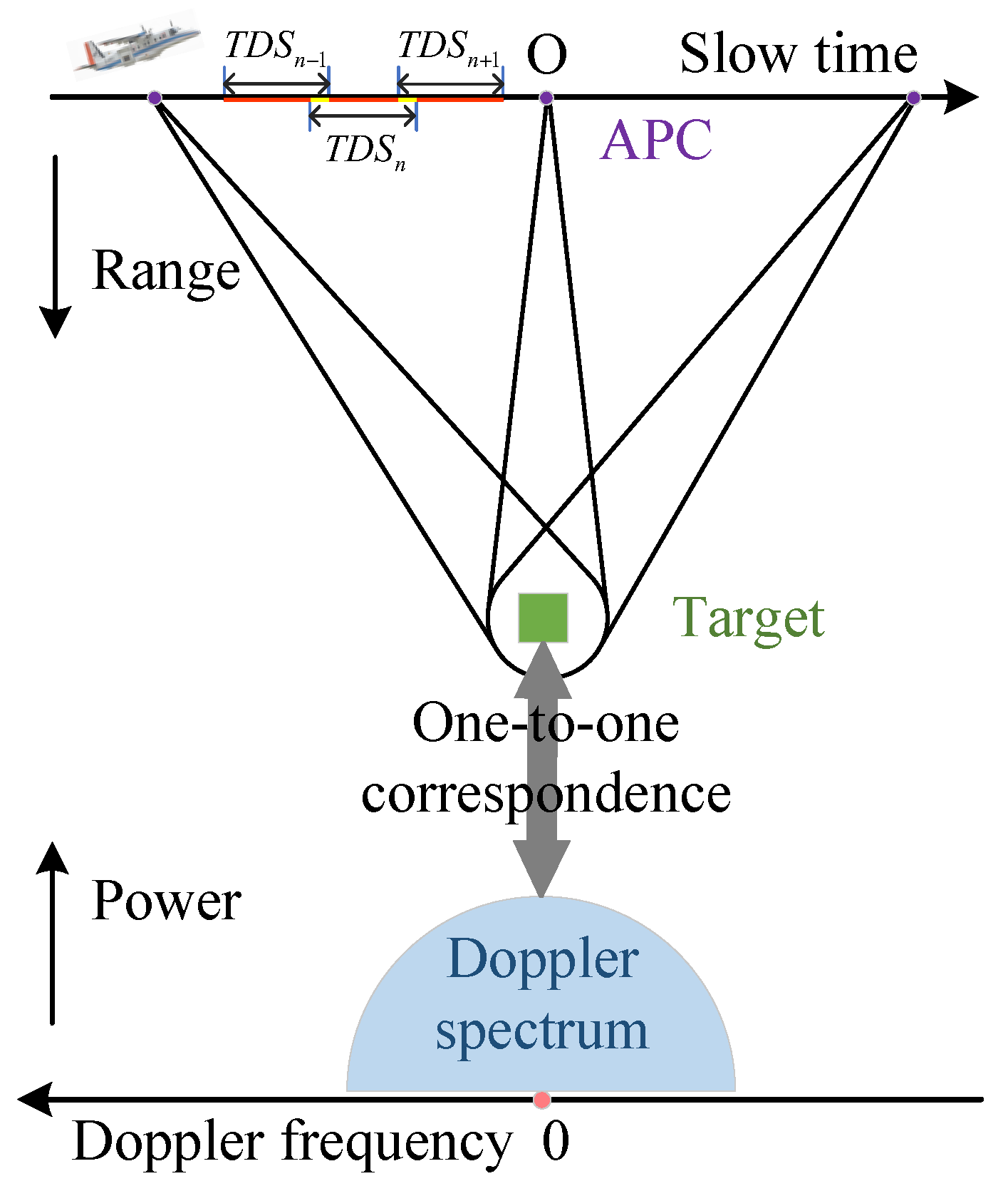
2. Geometric Model of Spotlight ViSAR and Problem Statement
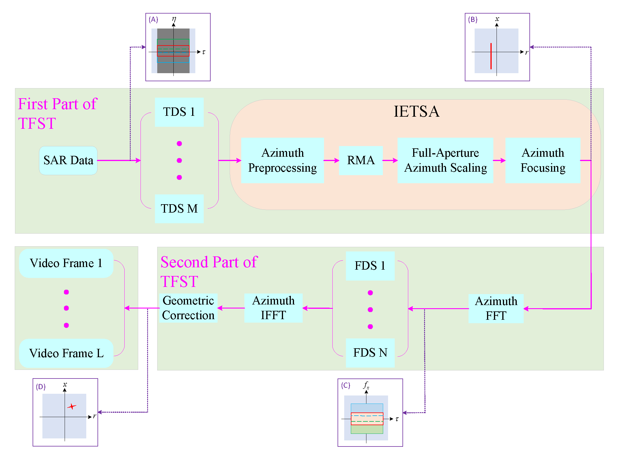
The ViSAR system operating in staring spotlight-mode can illuminate the same area continuously using beam steering. It is not limited by the beam width, so it can achieve higher azimuth resolution and longer video observation times. Figure 1 shows the data acquisition geometry of staring spotlight-mode ViSAR. In this figure, the SAR sensor travels along the x-axis at an effective velocity v. R 0 is the closest range from the center of scene O to the trajectory. R ( η ) is the instantaneous slant range and η s t a r t and η e n d are the starting and ending times of the recording, respectively. θ s y n is the relative rotation angle between η s t a r t and η e n d . The length of A D is the full synthetic aperture length L s and B C is the sub-aperture length L v f (where L v f L s ) corresponding to a video frame. The value of L v f depends on the desired azimuth resolution ρ a of a video frame. Assuming that θ v f is the coherent integration angle corresponding to a video frame, then it can be expressed as [27]:
θ v f 2 a r c s i n λ c γ a , w 4 ρ a
where λ c is the central wavelength and γ a , w is the mainlobe-broadening factor introduced by windowing.
Assuming that the coordinates at azimuth times η B and η C are ( X b , Y b , Z b ) and ( X c , Y c , Z c ), respectively, then L v f can be approximately expressed as [28]:
L v f = m a x b + b 2 4 a c 2 a , b b 2 4 a c 2 a Y b
where
a = X b 2 c o s ( θ v f ) 2 + Y b 2 c o s ( θ v f ) 2 Y b 2 b = 2 X b 2 Y b c = X b 2 Y b 2 c o s ( θ v f ) 2 + X b 4 c o s ( θ v f ) 2 X b 4 ,
and X b = X c , Z b = Z c .
Spotlight mode has longer monitoring time than strip mode, is more practical than circular SAR and is easy to extend to spaceborne ViSAR. However, the large computational complexity limits the real-time monitoring of ViSAR. Therefore, an efficient ViSAR data processing algorithm suitable for spotlight mode is necessary.
In this paper, a novel TFST is proposed to improve the processing efficiency of high-resolution ViSAR data. In particular, TFST focuses on three main issues. First, due to the influence of atmospheric turbulence, it is necessary to compensate the motion error. In addition, in order to perform video monitoring for a long time and reduce the computational burden, it is necessary to be able to process slant spotlight SAR data with full aperture. Finally, a series of video frames can be efficiently acquired. Moreover, TFST is validated by simulation and experimental airborne X-band data.

3. Methods

It is assumed that the radar transmits a linear frequency-modulated (LFM) signal with a duration of T r . Then, the demodulated echoes of a TDS can be expressed as
s s ( τ , η ) = w r τ T r w a η T TDS · e x p j π K r τ 2 R ( η ) c 2 e x p j 4 π R ( η ) λ
where τ and η are the fast and slow times, c is the propagation speed of light, K r is the frequency modulation rate of the transmitted chirp signal, λ is the wavelength, T TDS is the azimuth duration corresponding to the TDS and w r ( · ) and w a ( · ) represent the envelope of the transmitted signal and the azimuth window function, respectively.
Then, the echo signal in the range frequency and azimuth time domains is given as follows.
S s ( f r , η ) = W r f r w a η T TDS × e x p j π f r 2 K r e x p j 4 π ( f c + f r ) R ( η ) c
where f r is the range frequency, f c is the central transmitted frequency and W r ( · ) is the Fourier transform of w r ( · ) .

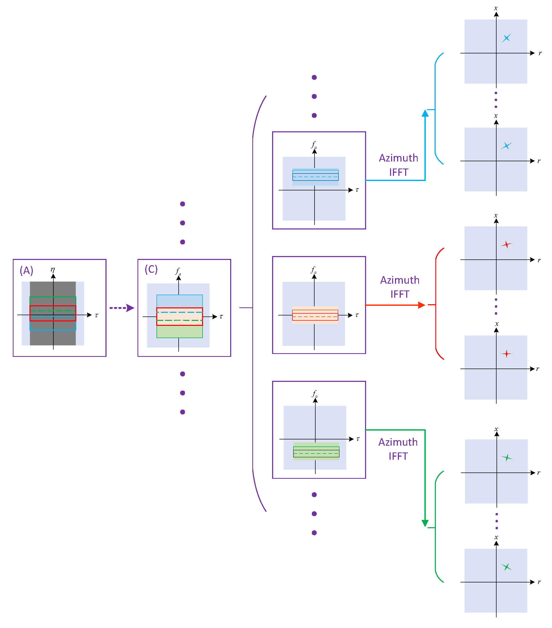
3.1. Azimuth Preprocessing in TFST

Lanari et al. [29,30] proposed the two-step approach (TSA) based on azimuthal time-domain convolution to solve the azimuthal aliasing problem of spotlight/sliding spotlight mode. The reference function used for azimuth deramping in TSA is
s r e f ( η ) = e x p j 2 π ( v η ) 2 R r e f f c c
where R r e f denotes the reference range and equals the closest approach R 0 of the scene center in the staring spotlight mode.
In the case of a large transmitted signal bandwidth, a significant deviation of the instantaneous range frequency from f c will cause the Doppler bandwidth after spectral analysis to be much larger the than pulse repetition frequency (PRF) [31,32]. Liu et al. [31] proposed to use a range-frequency-dependent reference function to mitigate this aliasing effect:
S r e f ( f r , η ) = e x p j 2 π ( v η ) 2 R r e f f c + f r c .
The range-frequency-dependent Doppler centroid of S s ( f r , η ) for the more generalized squinted SAR geometry was proposed in [22]:
f d c ( f r ) = 2 v s i n ( θ 0 ) ( f c + f r ) c
where θ 0 is the squint angle of the aperture center corresponding to a certain TDS and the nominal Doppler centroid is
f d c 0 = 2 v s i n ( θ 0 ) f c c .
Then, the azimuth time-domain convolution can be expressed as [22]
s a ( f r , η ) = T TDS / 2 T TDS / 2 S s ( f r , t ) · e x p j 2 π f d c t · S r e f f r , ( η t ) d t = S r e f ( f r , η ) · T TDS / 2 T TDS / 2 S s ( f r , t ) · e x p j 2 π f d c t · S r e f ( f r , t ) · e x p ( j 2 π K r o t η t ) d t
where
K r o t ( f r ) = 2 v 2 ( f c + f r ) c · R r e f .
The operation of (10) can be broken down into deramping, Fourier transform and phase compensation. Then, Fourier transform is applied on the azimuth time η to obtain the 2−D frequency spectrum S S a ( f r , f a )
S S a ( f r , f a ) = F F T s a f r , P R F N · K r o t m
where m = N 2 , , N 2 1 and N must satisfy
N P R F ( B b + B r o t + B s q ) K r o t 0
where B b = 2 v c o s ( θ 0 ) θ b w / λ c is the azimuth beam bandwidth, B r o t = | K r o t 0 | · T TDS is the Doppler bandwidth extended by steering of the beam, B s q = 2 v B r sin θ 0 / c is the squinted Doppler bandwidth and K r o t 0 is the nominal Doppler frequency modulation rate
K r o t 0 = 2 v 2 f c c · R r e f .
To correctly focus the signal of (12), two problems need to be solved. One is the non-uniform sampling of the azimuth spectrum due to the range-frequency-dependent K r o t [22]. The other is the significant range–azimuth coupling effect occurring in highly squinted SAR. The Doppler spectrum resampling proposed in [22] can solve the first problem, but cannot be used to overcome the second problem.
Although the range-azimuth coupling is weakened by (10), it is mainly aimed at the linear term of the range cell migration (RCM) and the real closest slant range of the target in the same range cell may be different; therefore, migration residuals still exist after RCM correction (RCMC). According to the principle of equivalent array in [23], in order to make the echo data received by the linear array (LA) and its equivalent array (EA) with a projection angle of θ 0 completely equivalent, the relationship between the Doppler frequency of LA and EA can be expressed as:
f a E A = c o s ( θ 0 ) 2 f a L A + v λ s i n ( θ 0 ) s i n ( θ 0 ) c o s ( θ 0 ) v λ 2 f a L A + v λ s i n ( θ 0 ) 2 ,
where f a L A and f a E A represent the Doppler frequencies of the echo data of LA and EA, respectively. Further, for high-resolution SAR data, considering the round-trip delay, it can be further expressed in the 2−D frequency domain as
f a n e w = c o s ( θ 0 ) 2 ( f a + f d c ) s i n ( θ 0 ) c o s ( θ 0 ) · 2 v ( f c + f r ) c 2 ( f a + f d c ) 2 ,
where f a n e w is the new azimuth frequency after azimuth resampling on (12) and
f a = k · Δ f a , k = ( N 2 , , N 2 1 ) ,
where
Δ f a = ( | K r o t | P R F ) .
Then, the equivalent new PRF is
P R F n e w = m a x f a n e w m i n f a n e w .
where m a x ( · ) and m i n ( · ) represent the maximum and minimum operators, respectively.
After azimuth resampling, the classic broadside SAR imaging algorithm can be used to focus the squint SAR data [23]. Next, it will be explained how the azimuth resampling completes the uniform sampling of (12).
From [22], we know that in order to align the sampling grids, we need to implement the following change of variables:
k · Δ f a + f d c = k · Δ f a 0 + f d c 0
where
Δ f a 0 = | K r o t 0 | P R F .
After azimuth resampling, the squint angle θ 0 is equal to 0 [23], so f d c = f d c 0 ≡ 0. In addition, f a n e w can be generated at equal intervals according to (16). The 2−D spectrum S S a ( f r , f a ) can then be resampled in azimuth to align the sampling grids:
S S a ( f r , k · Δ f a ) S S a ( f r , k · Δ f a n e w )
where Δ f a n e w = P R F n e w / N .
Therefore, after azimuth resampling the 2−D spectrum is sampled uniformly and is equivalent to the spectrum of the broadside mode, as shown in Figure 2. The corresponding simulation parameters are listed in Table 1. Comparing Figure 2a,b, the signal spectrum after azimuth resampling is equivalent to the broadside SAR. At the same time, the effective velocity v is transformed into v c o s ( θ 0 ) .
Then, the product of the 2−D spectrum S S a ( f r , f a n e w ) and the frequency domain phase compensation function S c o m will be the same as the spectrum of a broadside SAR:
S S ( f r , f a n e w ) = S S a ( f r , f a n e w ) · S c o m
where
S c o m = e x p j π · ( f ^ a n e w ) 2 K r o t
Therefore, the existing broadside imaging algorithm can be used to process the data [23]. According to (16), f ^ a n e w can be expressed as
f ^ a n e w = f a n e w + s i n ( θ 0 ) · | B A 2 | f d c
where
B = f a n e w c o s ( θ 0 ) ,
and
A = 2 v · ( f c + f r ) c 2 .
Next, the classical frequency domain algorithm RMA can be used to accomplish range cell migration (RCM) correction and range compression. In this manner, we can obtain s S r c m c ( R ( η ) , f a n e w ) for azimuth scaling, where R ( η ) is the slant range, not the closest approach defined in [22].

3.2. Modified Full-Aperture Azimuth Scaling

It is necessary to solve the problem of slow time-domain aliasing of high-resolution SAR data using TSA. Zhu et al. [22] developed a full-aperture azimuth scaling technique based on the azimuth scaling of [33,34,35] and combined motion compensation (MoCo) and autofocusing [34,36], which can effectively solve this problem. However, the processing here is based on the signal obtained after azimuth resampling, which is different from the Doppler Spectrum Resampling in [22], so the full-aperture azimuth scaling needs further modification.
Similar to sub-aperture azimuth scaling, full-aperture azimuth scaling can be expressed as [22]
β ( R , η ) = F 1 s S ( R , f a n e w ) · e x p j π K a ( R s c l ) · η 2
where F 1 is the inverse Fourier transform, R s c l is the reference range and
s S ( R , f a n e w ) = s S r c m c ( R , f a n e w ) · e x p j 4 π λ · R · D ( f a n e w ) 1 · e x p j π f a n e w 2 K a ( R s c l ) ,
and
D ( f a n e w ) = 1 λ 2 · f a n e w 2 4 v 2 ,
and
K a ( R s c l ) = 2 v 2 λ · R s c l .
Then, as detailed in Appendix A, the dechirped signal for slow time-domain error compensation is obtained by applying the IFFT to (A4) and can be expressed as
β ( R , k · Δ η ) = IFFT Γ ( R , k · Δ f a n e w ) .
where Δ η = Δ F a n e w / K a ( R s c l ) is the sampling interval of the slow time domain.
Figure 3 shows the specific flow diagram of azimuth scaling and slow time domain error compensation and the scaling function used in the proposed algorithm is [22]
H s c l ( f a n e w ) = e x p j π K a ( R s c l ) ( δ 1 ) f a n e w 2
where δ = R s c l / R , the phase perturbation function is
H p h p ( η n e w ) = e x p j π K a ( R s c l ) δ η n e w 2
where
η n e w = k P R F n e w
and the inverse scaling function H i n s ( f a n e w ) is the conjugate of H s c l ( f a n e w ) .

3.3. Motion Error Compensation in TFST

In addition, since airborne SAR is susceptible to atmospheric turbulence, motion compensation is essential. First, according to the motion compensation scheme proposed in [37], the phase error and envelope displacement between the real and ideal trajectories are compensated by using inertial navigation system and inertial measurement unit (INS/IMU) measurements.
The residual phase error after MOCO using INS/IMU data is
Φ e f r , η = e x p ( j 4 π c f c + f r Δ R η ) ,
where Δ R η is the slope range residual error. After azimuth preprocessing, it can be expressed as [23]
Φ e f r , η n e w = e x p ( j 4 π c f c + f r Δ R ξ ( η n e w ) ) ,
where ξ ( η n e w ) is a function of η n e w and its analytical relationship does not need to be considered here.
Then, through the modified full-aperture azimuth scaling processing, the traditional PGA [38] can be used to estimate the residual phase error and the specific motion compensation process is shown in Figure 4.

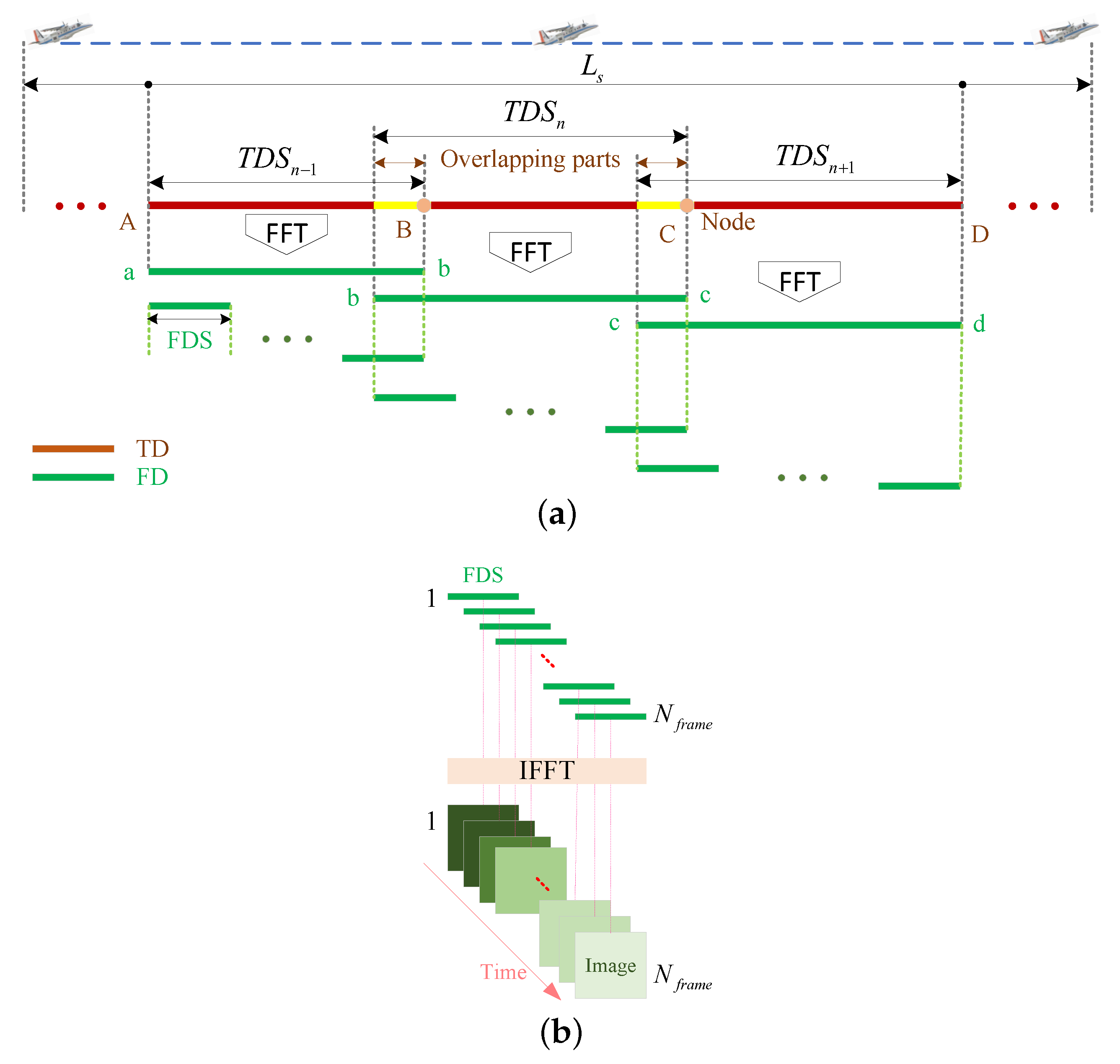
3.4. Fundamentals of TFST

Different from traditional sub-aperture methods [6,8,29,30], in our method the TDS is required to be as large as possible, as shown in Figure 5. In addition, Figure 6 shows the corresponding relationship between TDS and FDS. It shows how to concatenate the video frame sequence formed by multiple TDSs. In the experimental data processing, the TDSs are sequentially processed by sliding in the time domain and multiple FDSs are generated in the frequency domain to form a series of video frames. In particular, T D S n represents the nth TDS and the segment marked in yellow represents the overlapping parts (OPs) between T D S n and its two adjacent TDSs, to ensure that video frames formed by multiple TDSs can be smoothly connected.
Moreover, it is necessary to analyze the influence of the OPs on the amount of calculations. We performed an experiment with the parameters shown in Table 1. Figure 7 shows the ratio of OPs to TDSs with a coherent integration angle of 10° and a range resolution of ρ r = 0.1249 m. Owing to the very high range resolution, even if ρ a / ρ r is 7, then ρ a = 0.8743 m, which is still less than 1 m. Referring to Figure 7a, it can be seen that the amount of calculations incurred by the OPs is tiny. Furthermore, comparing to Figure 7a,b, it can be found that the influence of OPs on Ka-band ViSAR is almost negligible, which reveals the application potential of the proposed algorithm.
The complete flow diagram of high-resolution ViSAR data processing is shown in Figure 8 and it consists of two main steps: TDS processing, which corresponds to the first part of TFST and FDS processing, which corresponds to the second part of TFST. In (A), the areas marked by red, green and blue boxes, respectively, illustrate the division of TDS in a two-dimensional time domain, which corresponds to Figure 5. Next, M TDSs can be processed by IETSA in parallel and the output is shown in (B). Corresponding to (A), (C) shows the division of N FDSs. Moreover, a geometric correction is applied to remove the distortion introduced by azimuth resampling [23]. The final output is shown in (D); thus, a series of video frames for generating video are obtained.
To further explain TFST, the time-frequency diagram of the formation of multiple video frames is shown in Figure 9. It can be seen that multiple video frames of desired resolution can be obtained without sub-aperture reconstruction.
Next, the specific parameter design scheme is given. The synthetic aperture time corresponding to the l-th FDS is
T FDS , l = R 0 t a n ( θ s t a r t , l ) t a n ( θ e n d , l ) v ,
so, the frame rate can be expressed as follows
F = 1 T FDS · 1 α .
where l = 1 , , N f r a m e and N f r a m e is the total number of FDSs, θ s t a r t , l and θ e n d , l are the start and end squint angles corresponding to the l-th FDS and α is the overlap rate. In practice, to obtain the minimum frame rate, we can use the maximum value of T FDS , l for T FDS .
The Doppler bandwidth corresponding to an FDS is [39]
B d o p = 2 v cos θ r c λ c θ v f .
where θ r c is the squint angle at the center of the aperture.
It can be seen that for a fixed frame-length ViSAR, the θ v f of different FDSs is slightly different due to the change in the squint angle. In practice, the frame-length, B d o p , is obtained at the aperture center.
Then, the overlap rate α is obtained using (39) and the desired frame rate. Therefore, a series of FDSs can be formed in the Doppler domain, as shown in Figure 8 and Figure 9.
In application, for airborne ViSAR, multiple different video frames need to be registered before forming video. Thus, geometric correction can be solved through registration processing, which will not increase the amount of calculation of registration, but reduce the complexity of TFST, which can further improve the efficiency.

3.5. Complexity Analysis of TFST

TFST includes two main steps: TDS processing and FDS processing, as shown in Figure 8. It is assumed that the dimensions of SAR data in range and slow time are N r and N a , respectively, and all operations can be divisible. Then, the size of a TDS is N a m × N r and N a m = N a / M . A complex multiplication requires a total of six floating-point operations. A 1D FFT with length N requires 5 N l o g 2 N flops and an N × N 2−D FFT requires 10 N 2 l o g 2 N flops. The interpolation operation with core length N k e r requires ( 2 N k e r 1 ) flops per complex output point and N k e r is generally 8 or 16 in practice [39]. For convenience of analysis, let N a m = N r N .
IETSA in TDS processing includes four main operations: complex phase multiplication, 1D FFT, 2−D FFT and interpolation, so the amount of operation is O ( N 2 ) + O ( N l o g 2 N ) + O ( N 2 l o g 2 N ) + O ( ( 2 N k e r 1 ) N 2 ) . FDS processing includes two main operations: 1D FFT and interpolation, so the amount of operation is O ( N l o g 2 N ) + O ( ( 2 N k e r 1 ) N 2 ) . Therefore, the total complexity of TFST is O ( N 2 ) + O ( N l o g 2 N ) + O ( N 2 l o g 2 N ) . The complexity of BP is O ( N 3 ) , which is obviously larger than that of TFST.
To sum up, TFST is more practical in high-resolution ViSAR data processing due to its accuracy and high efficiency.

4. Results and Discussion

In this section, the proposed method is evaluated through simulations and experiments and the results are analyzed in depth. Moreover, the parameters not mentioned in the simulation are the same as those in Table 1. The data comes from the X-band airborne SAR system of the Aerospace Information Research Institute, Chinese Academy of Sciences (AIRCAS), and the transmission signal bandwidth is 1.2 GHz.

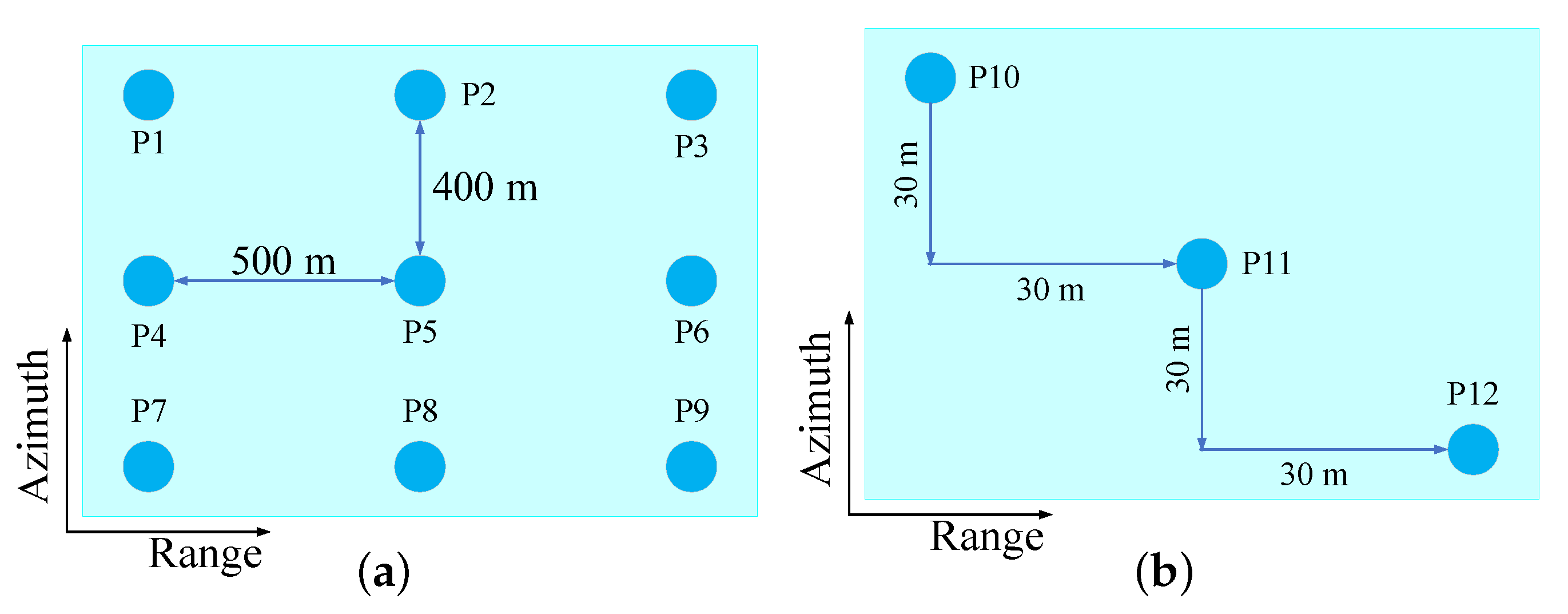
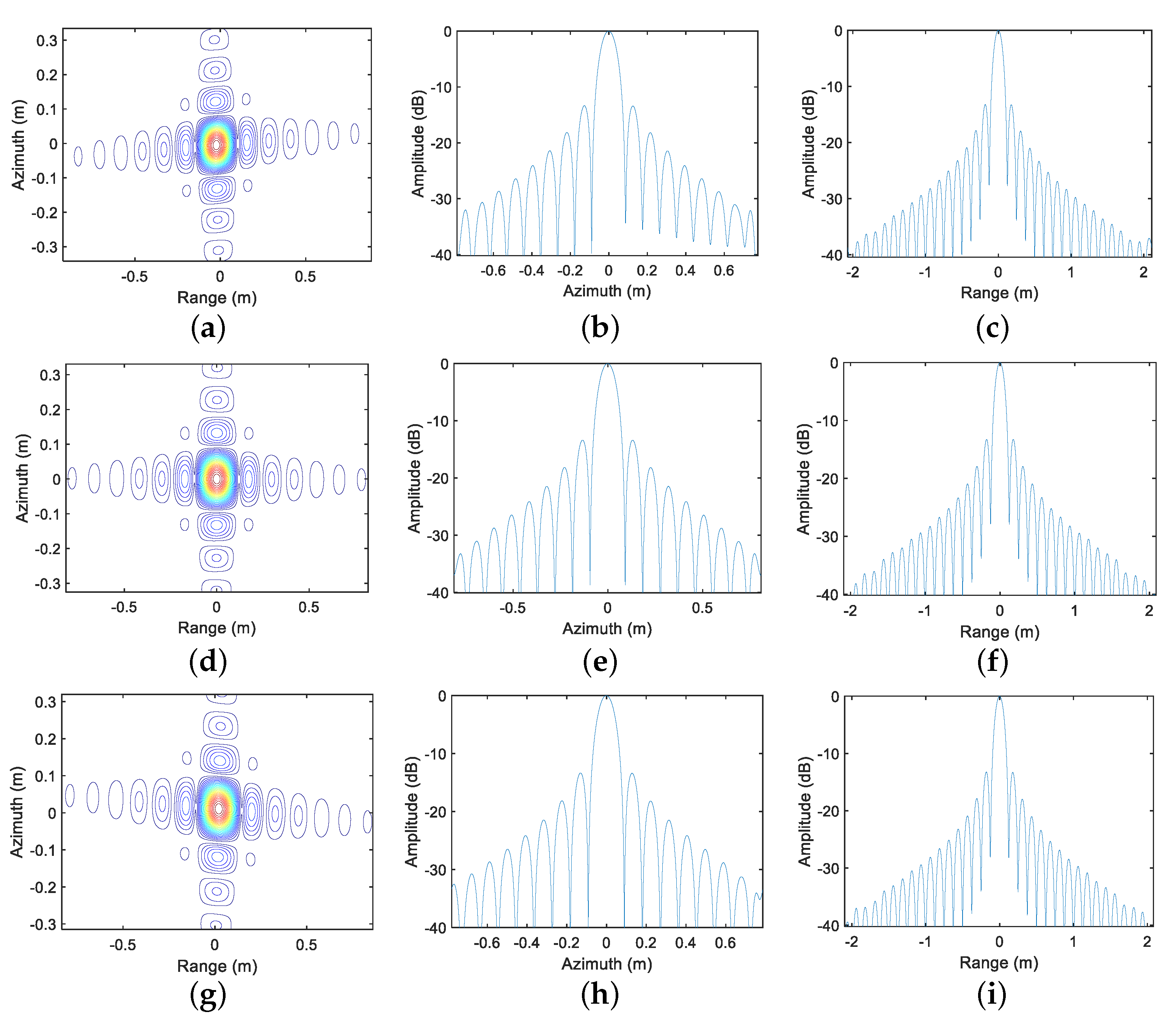
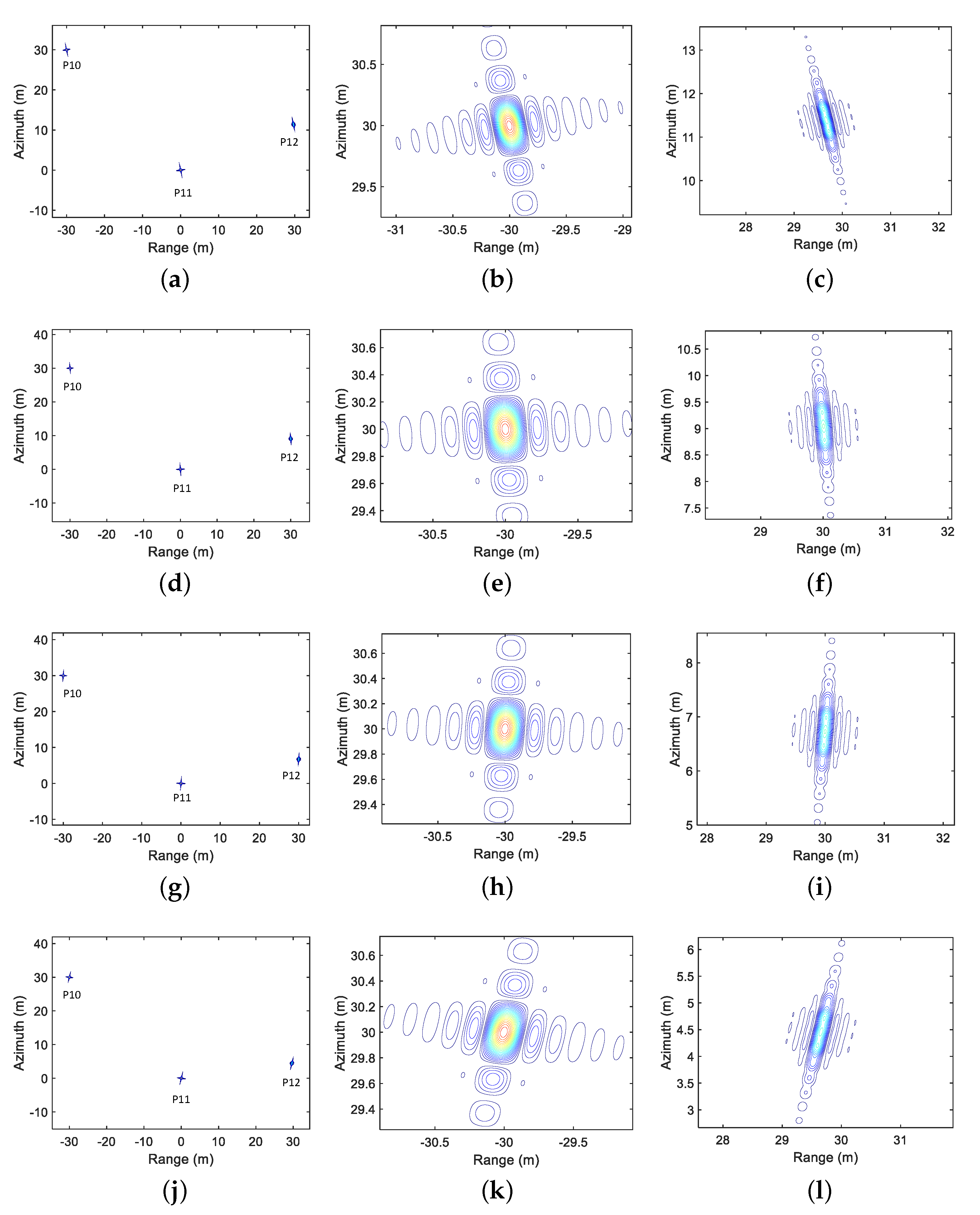
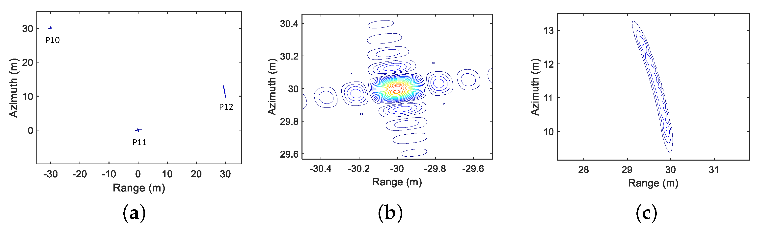
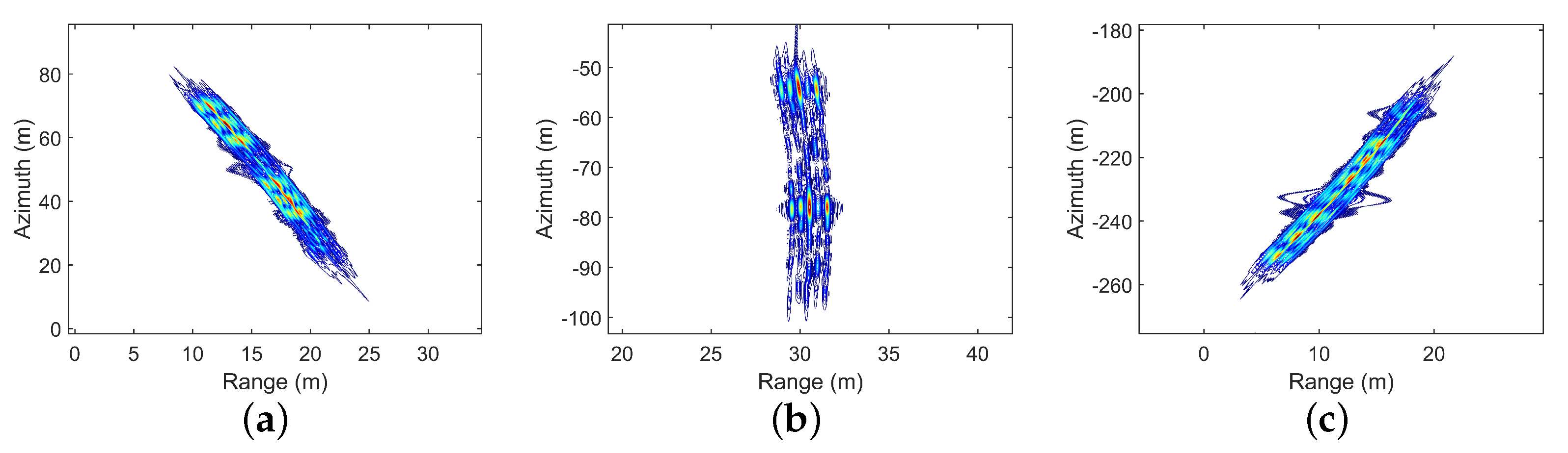
4.1. Simulation Results and Discussion

Figure 10 shows the geometric distribution of point targets in ground scene. To verify the IETSA, the case of a coherent integration angle of 10° and a squint angle of 15° is analyzed. In particular, the simulation results of the three-point targets P1, P5 and P9 in Figure 10a are analyzed, as shown in Figure 11, and the peak sidelobe ratio (PSLR), the integrated sidelobe ratio (ISLR) and the resolution achieved are summarized in Table 2. Combined with Figure 11 and Table 2, it can be concluded that the three point targets are well focused, which confirms that IETSA can effectively focus squint spotlight SAR data. This is a key step to improving the practicability of TFST.
In addition, the comparison results of ETSA [22] and IETSA are shown in Figure 12. The coherent integration angle and squint angle used in the simulation are 5° and 7.2°, respectively. It can be seen that for the squint mode SAR data, IETSA has better focusing performance than ETSA and the phase error caused by azimuth resampling can be compensated by TFST.
Different from IETSA simulation, for the verification of TSFT, we designed a scene with three-point targets, as shown in Figure 10b, which includes two stationary point targets P10 and P11 and and a moving target P12 whose azimuth and range speeds are −0.4 m/s and −0.1 m/s, respectively. The parameters used for TFST verification are shown in Table 3.
The simulation results of TFST are shown in Figure 13 and Figure 13a is frame 49, with a squint angle of 10.17°, Figure 13b is frame 148, with a squint angle of 3.25°, Figure 13c is frame 246, with a squint angle of −3.69° and Figure 13d is frame 344, with a squint angle of −10.40°. The first column is the result for the entire scene, while the second and third columns are the enlarged results of P10 and P12 from the first column, respectively.
The second column of Figure 13 shows that the position of point target P10 in the different video frames is fixed. However, the position of moving target P12 varies among different frames, which confirms that ViSAR has the ability to discern moving targets.
To further evaluate the focusing performance of ViSAR, the point target P10 was analyzed in different frames and the PSLR, ISLR and the resolution are summarized in Table 4. It can be seen that the change in the azimuth resolution of different frames is minimal.
Figure 14 shows the simulation results of the traditional SAR, with a squint angle of 10° and a coherent integration angle of 10°. Comparing the point target P12 in Figure 14 and Figure 13, it is evident that the moving target appears as a defocused line target in the traditional SAR image, which cannot show the dynamic change characteristics. However, ViSAR images can illustrate whether a target is moving, which is more helpful for moving target detection.
In addition, a distributed target (DT) with a size of 4 × 2 m is simulated, whose velocities in azimuth and range are −8 m/s and −1 m/s, respectively. The simulation results of DT are shown in Figure 15. The time interval between Figure 15a,b is about 15 s and that between Figure 15b,c is about 19 s. According to Figure 15, it can be seen that the azimuth and range position of DT both change with time and the imaging result is seriously defocused. Compared with Figure 13, the defocus and displacement of the moving target in Figure 15 are larger because of its greater velocity. Simulation of DT reveals how moving targets appear in real scenes.

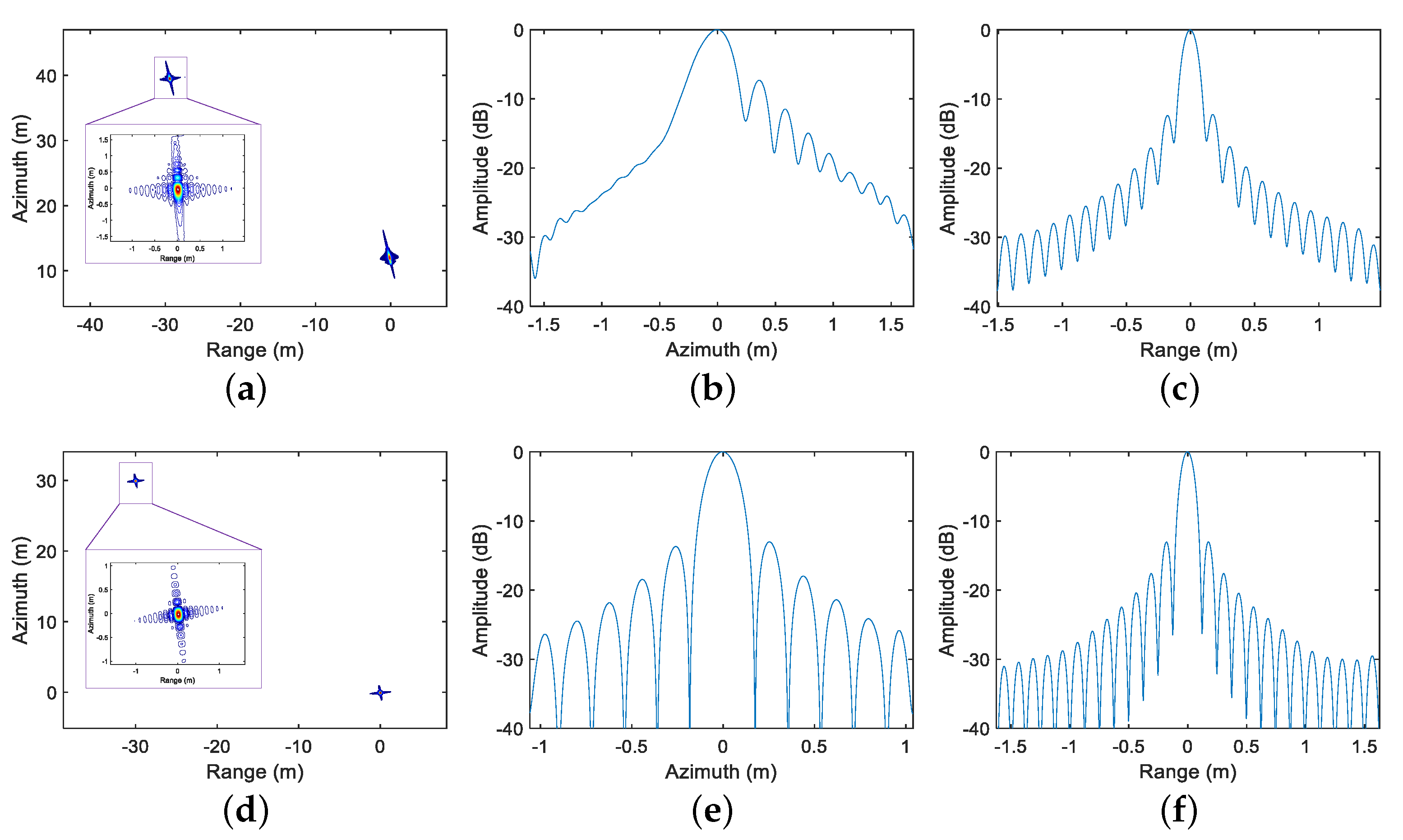
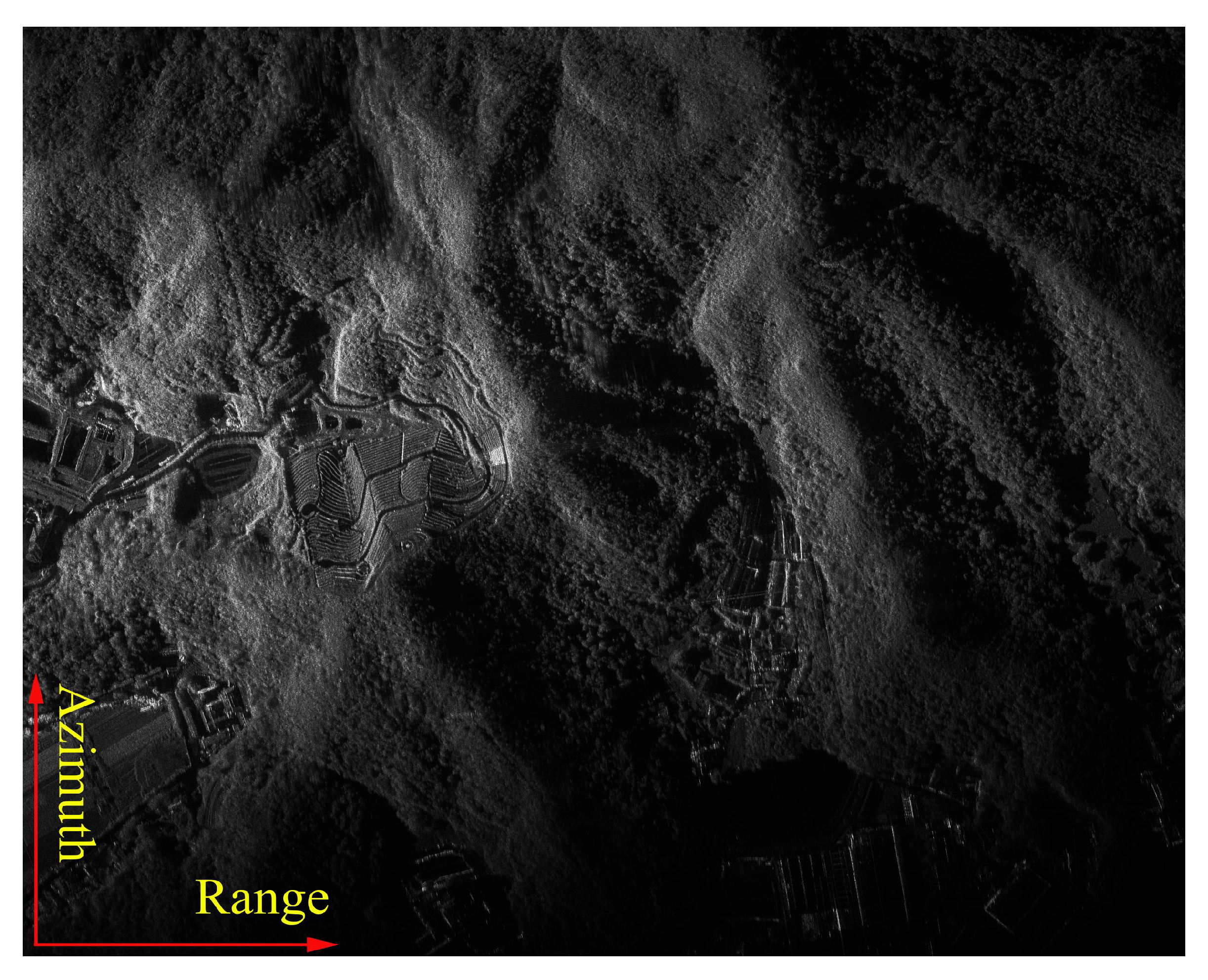
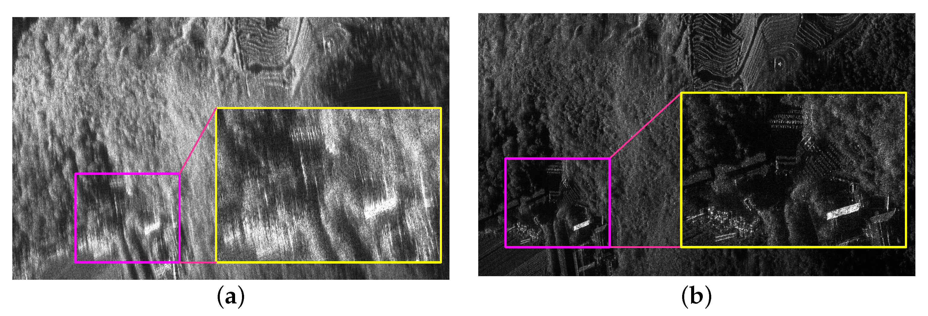
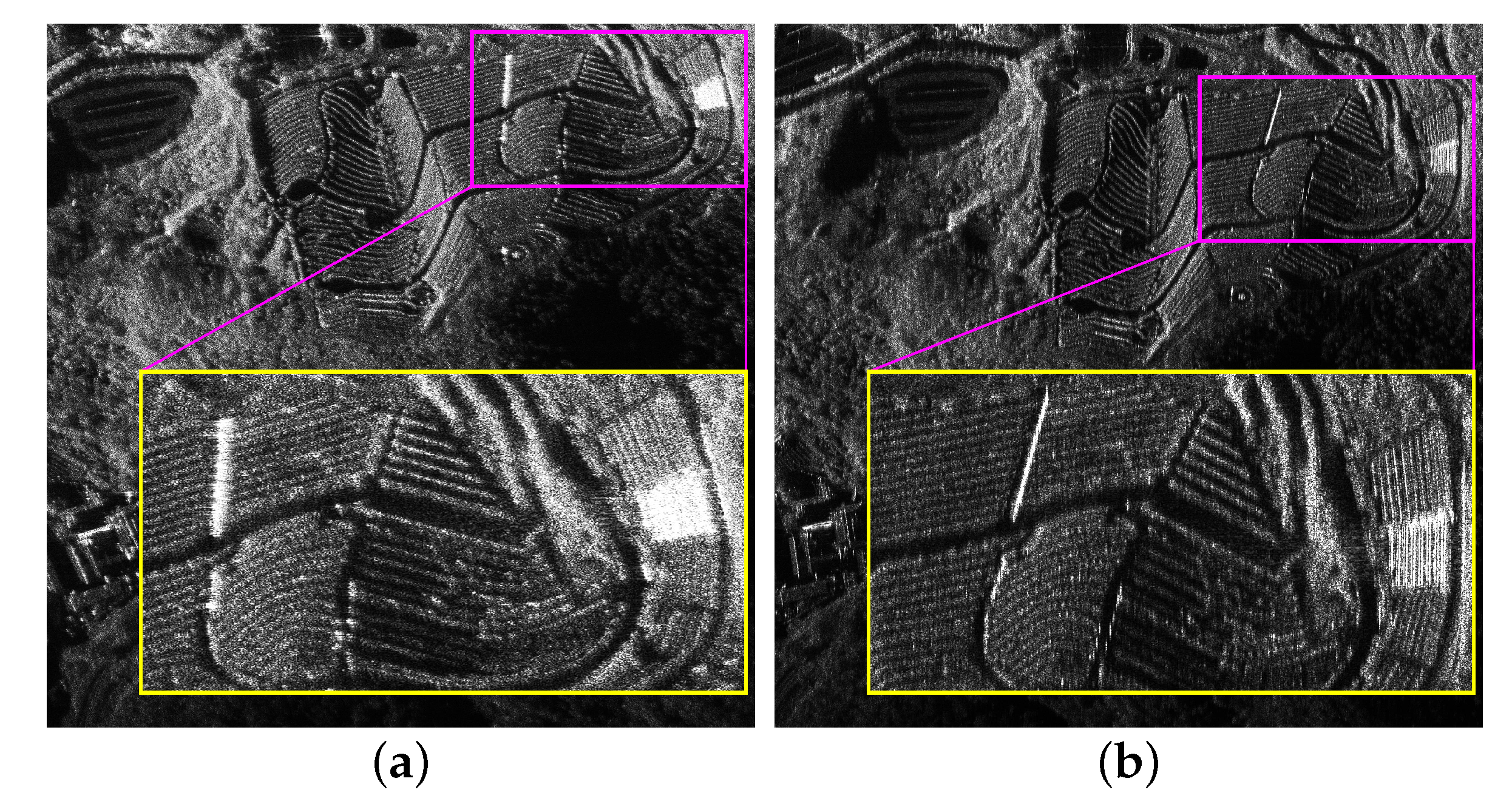
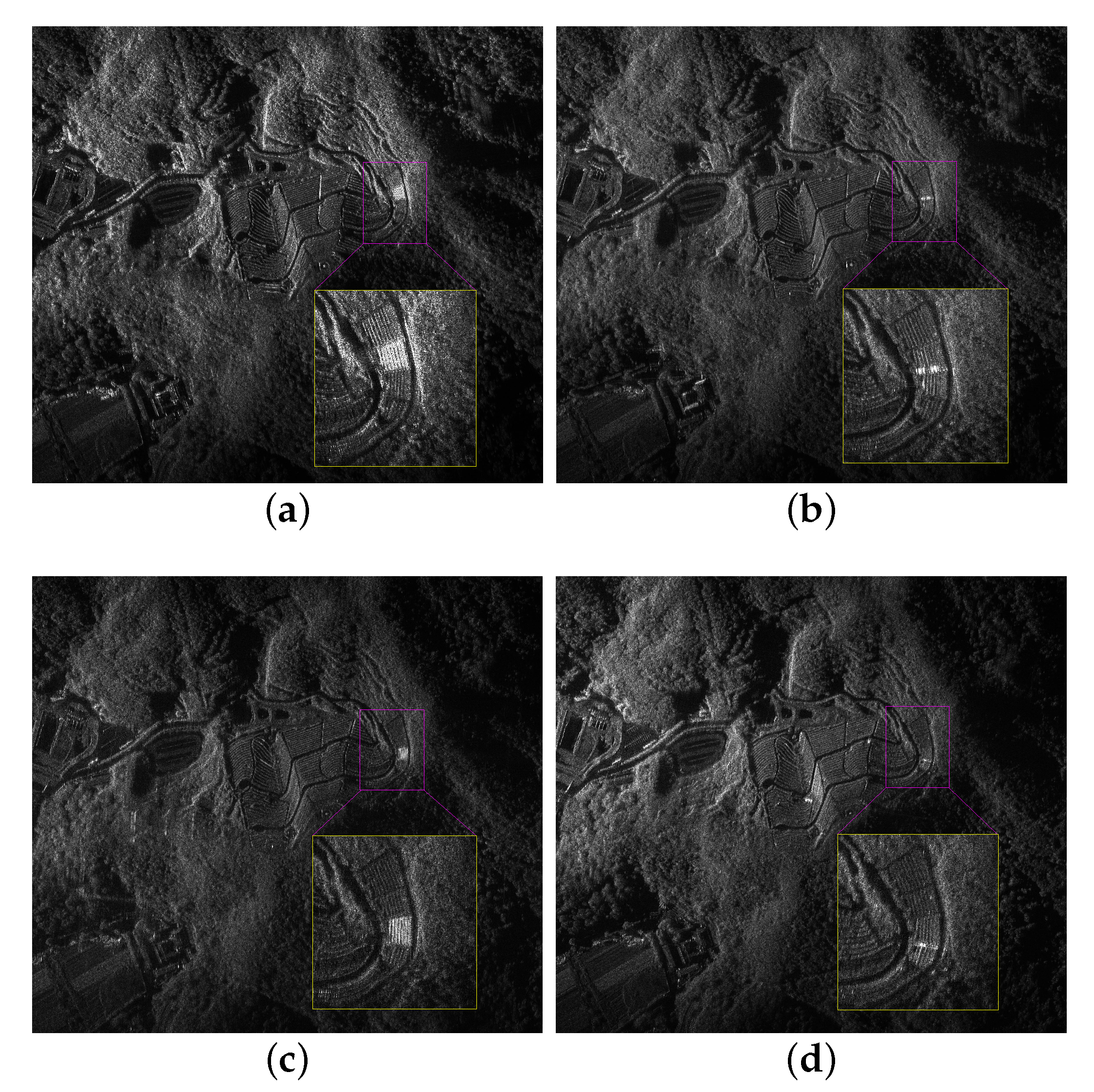
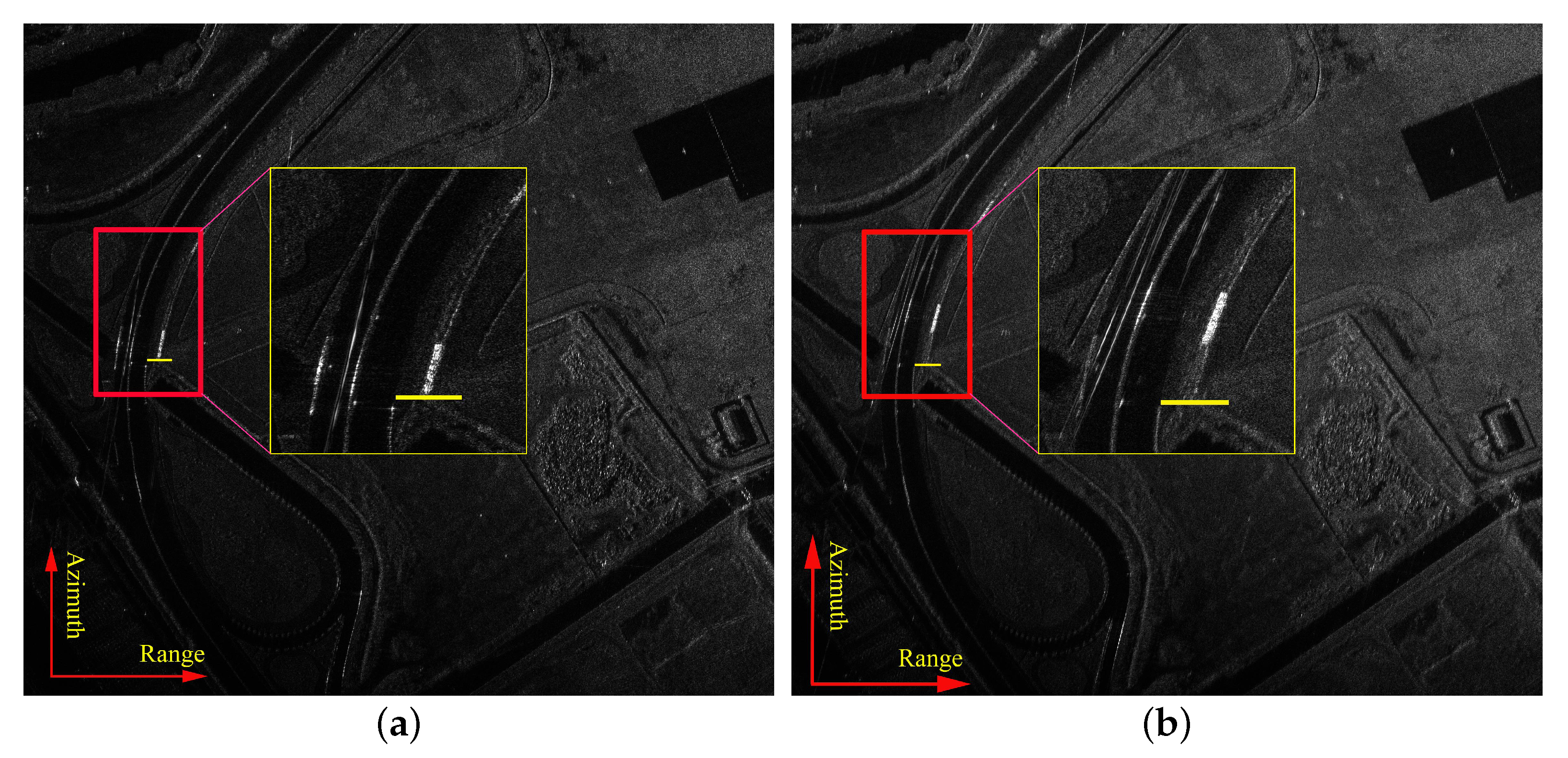
4.2. Airborne SAR Data Results and Discussion

A continuation of the discussion based on the X-band airborne SAR data from AIRCAS and the focused SAR image processed using IETSA is shown in Figure 16, with a squint angle of 10° and a coherent integration angle of 10°, which further confirms the effectiveness of IETSA.
Moreover, Figure 17 presents the experimental data processing results of ETSA and IETSA. It is obvious that the focusing quality of IETSA is better, which is the same as the conclusion in Figure 12. At the same time, we also confirmed by the experimental data that TFST can compensate the phase error caused by azimuth resampling.
Further, to illustrate that TFST has better performance, Figure 18 shows the comparison results of TFST and Doppler Shifting Technique (DST) proposed by [10]. In particular, Figure 18 corresponds to a video frame at an intermediate moment generated from data with a squint angle and a coherent integration angle of 11° and 8°, respectively. It can be seen that the focus quality of TFST is better compared to DST.
Then, the X-band airborne SAR data within [15°, −15°] were processed with the method shown in Figure 8 at a fixed frame rate of 2.3687 Hz. The range resolution was 0.1249 m and the azimuth resolution of the middle video frame was set to 0.2379 m. Due to FDS processing in fixed frame length mode, the resolution of different video frames will vary slightly. Nonetheless, according to the simulation results in Table 4, these changes are negligible.
The processing results of TFST are shown in Figure 19 and Figure 20. Figure 19 shows video frames at four different times of the area in Figure 16, from which it can be inferred that the aircraft is moving from bottom to top along the azimuth. The result shows that ViSAR can acquire images from multiple angles of the same target, which is helpful for image information interpretation. Moreover, Figure 20 is an urban scene and there is a road on the left. Comparing Figure 20a and Figure 20b, it is evident that the bright line in the area marked by the red rectangle is a moving target. Its position has shifted and the imaging result is seriously defocused. This is consistent with the simulation results of DT in Figure 15. In addition, the background of the ViSAR image is static and the position of the stationary target is constant, so the target whose position changes significantly in different video frame images should be a dynamic target. This result demonstrates the potential of ViSAR for moving target indication (MTI).
It is worth emphasizing that, according to (39), a higher frame rate can be obtained by adjusting the overlap rate and the resolution of the video frame. In practice, these three variables need to be considered comprehensively to reduce the amount of calculations as much as possible.

5. Conclusions

In this paper, we first propose an IETSA approach based on azimuth resampling and full-aperture azimuth scaling, which allows squint spotlight SAR data processing at full aperture. Then, combining TDS processing and FDS processing, a novel high-resolution ViSAR data processing technique is proposed, which is called TFST.
Moreover, since TFST is based on RMA, the image quality can be guaranteed while improving the efficiency. These advantages make the TFST a more practical choice in the high-resolution ViSAR data processing.
In addition, the effect of azimuth resampling on motion error compensation is also analyzed and the results show that azimuth resampling will not reduce the imaging quality of TFST, suggesting the high practicability of TFST.
Finally, the effectiveness of the proposed method has been confirmed by simulation and airborne SAR data processing results.

Author Contributions

Conceptualization, C.Y.; Funding acquisition, Y.D., W.W., P.W. and F.Z.; Investigation, C.Y., Z.C., W.W. and F.Z.; Methodology, C.Y.; Project administration, W.W., P.W. and F.Z.; Resources, Y.D., W.W., P.W. and F.Z.; Validation, C.Y. and W.W.; Writing—original draft, C.Y.; Writing—review & editing, Z.C., Y.D., W.W. and F.Z. All authors have read and agreed to the published version of the manuscript.

Funding

This work was supported in part by the National Science Fund under Grant 61971401 and in part by the Youth Innovation Promotion Association, Chinese Academy of Sciences (CAS).

Data Availability Statement

Not applicable.

Acknowledgments

The authors would like to thank the Department of Space Microwave Remote Sensing System, Aerospace Information Research Institute, Chinese Academy of Sciences for providing X-band high-resolution SAR data.The authors would also like to thank all colleagues who participated in this experiment.

Conflicts of Interest

The authors declare no conflict of interest.

Appendix A

The convolution in the time (frequency) domain is equal to multiplication in the frequency (time) domain [39], so (28) can be expressed as
Γ ( R , f a n e w ) = s S ( R , f a n e w ) e x p j π f a n e w 2 K a ( R s c l )
Then, the convolution in (28) can be expanded as
Γ ( R , f a n e w ) = P R F n e w / 2 P R F n e w / 2 s S ( R , μ ) · e x p j π ( f a n e w μ ) 2 K a ( R s c l ) d μ = e x p j π f a n e w 2 K a ( R s c l ) · P R F n e w / 2 P R F n e w / 2 s S a s ( R , μ ) · e x p j 2 π f a n e w K a ( R s c l ) μ d μ
where
s S a s ( R , μ ) = s S r c m c ( R , μ ) · e x p j 4 π λ · R · D ( μ ) 1 .
Expressing (A2) in discrete form, we obtain:
Γ ( R , k · Δ f a n e w ) = e x p j π K a R s c l · k P R F n e w 2 · IFFT s S a s ( R , k · Δ f a n e w ) .

References

  1. Curlander, J.C.; McDonough, R.N. Synthetic Aperture Radar; Wiley: New York, NY, USA, 1991; Volume 11. [Google Scholar]
  2. Soumekh, M. Synthetic Aperture Radar Signal Processing; Wiley: New York, NY, USA, 1999; Volume 7. [Google Scholar]
  3. Stilla, U. High resolution radar imaging of urban areas. In Proceedings of the Photogrammetric Week; Wichmann Verlag: Heidelberg, Germany, 2007. [Google Scholar]
  4. Moreira, A.; Prats-Iraola, P.; Younis, M.; Krieger, G.; Hajnsek, I.; Papathanassiou, K.P. A tutorial on synthetic aperture radar. IEEE Geosci. Remote. Sens. Mag. 2013, 1, 6–43. [Google Scholar] [CrossRef] [Green Version]
  5. Wells, L.; Sorensen, K.; Doerry, A.; Remund, B. Developments in SAR and IFSAR systems and technologies at Sandia National Laboratories. In Proceedings of the 2003 IEEE Aerospace Conference Proceedings (Cat. No. 03TH8652), Big Sky, MT, USA, 8–15 March 2003; Volume 2, pp. 2_1085–2_1095. [Google Scholar]
  6. Damini, A.; Balaji, B.; Parry, C.; Mantle, V. A videoSAR mode for the X-band wideband experimental airborne radar. In Proceedings of the Algorithms for Synthetic Aperture Radar Imagery XVII; International Society for Optics and Photonics: Bellingham, WA, USA, 2010; Volume 7699, p. 76990E. [Google Scholar]
  7. Miller, J.; Bishop, E.; Doerry, A. An application of backprojection for video SAR image formation exploiting a sub-aperature circular shift register. In Proceedings of the Algorithms for Synthetic Aperture Radar Imagery XX; International Society for Optics and Photonics: bellingham, WA, USA, 2013; Volume 8746, p. 874609. [Google Scholar]
  8. Song, X.; Yu, W. Processing video-SAR data with the fast backprojection method. IEEE Trans. Aerosp. Electron. Syst. 2016, 52, 2838–2848. [Google Scholar] [CrossRef]
  9. Hu, R.; Min, R.; Pi, Y. A video-SAR imaging technique for aspect-dependent scattering in wide angle. IEEE Sens. J. 2017, 17, 3677–3688. [Google Scholar] [CrossRef]
  10. Kim, C.K.; Azim, M.T.; Singh, A.K.; Park, S.O. Doppler Shifting Technique for Generating Multi-Frames of Video SAR via Sub-Aperture Signal Processing. IEEE Trans. Signal Process. 2020, 68, 3990–4001. [Google Scholar] [CrossRef]
  11. Huang, X.; Xu, Z.; Ding, J. Video SAR image despeckling by unsupervised learning. IEEE Trans. Geosci. Remote. Sens. 2020, 59, 10151–10160. [Google Scholar] [CrossRef]
  12. Hartmann, F.; Sommer, A.; Pestel-Schiller, U.; Ostermann, J. A scheme for stabilizing the image generation for VideoSAR. In Proceedings of the EUSAR 2021, 13th European Conference on Synthetic Aperture Radar, Online, 29–31 April 2021; pp. 1–5. [Google Scholar]
  13. Bishop, E.; Linnehan, R.; Doerry, A. Video-SAR using higher order Taylor terms for differential range. In Proceedings of the 2016 IEEE Radar Conference (RadarConf); IEEE: New York, NY, USA, 2016; pp. 1–4. [Google Scholar]
  14. Soumekh, M. Time Domain Non-Linear SAR Processing; Technical Report; State University of New York at Buffalo Department of Electrical Engineering: Buffalo, NY, USA, 2006. [Google Scholar]
  15. Frey, O.; Magnard, C.; Ruegg, M.; Meier, E. Focusing of airborne synthetic aperture radar data from highly nonlinear flight tracks. IEEE Trans. Geosci. Remote. Sens. 2009, 47, 1844–1858. [Google Scholar] [CrossRef] [Green Version]
  16. McCorkle, J.W.; Rofheart, M. Order N 2 log (N) backprojector algorithm for focusing wide-angle wide-bandwidth arbitrary-motion synthetic aperture radar. In Proceedings of the Radar Sensor Technology; International Society for Optics and Photonics: Bellingham, WA, USA, 1996; Volume 2747, pp. 25–36. [Google Scholar]
  17. Xiao, S.; Munson, D.C.; Basu, S.; Bresler, Y. An N 2 logN back-projection algorithm for SAR image formation. In Proceedings of the Conference Record of the Thirty-Fourth Asilomar Conference on Signals, Systems and Computers (Cat. No. 00CH37154), Pacific Grove, CA, USA, 29 October–1 November 2000; Volume 1, pp. 3–7. [Google Scholar]
  18. Rogan, A.; Carande, R. Improving the fast back projection algorithm through massive parallelizations. In Proceedings of the Radar Sensor Technology XIV; International Society for Optics and Photonics: Bellingham, WA, USA, 2010; Volume 7669, p. 76690. [Google Scholar]
  19. Jian, L.; Running, Z.; Lixiang, M.; Zheng, L.; Ke, J.; Dawei, W.; Zhiyun, T. An efficient image formation algorithm for spaceborne video SAR. In Proceedings of the IGARSS 2018-2018 IEEE International Geoscience and Remote Sensing Symposium, Valencia, Spain, 22–27 July 2018; pp. 3675–3678. [Google Scholar]
  20. Pu, W.; Wang, X.; Wu, J.; Huang, Y.; Yang, J. Video SAR imaging based on low-rank tensor recovery. IEEE Trans. Neural Netw. Learn. Syst. 2020, 32, 188–202. [Google Scholar] [CrossRef]
  21. Yamaoka, T.; Suwa, K.; Hara, T.; Nakano, Y. Radar video generated from synthetic aperture radar image. In Proceedings of the 2016 IEEE International Geoscience and Remote Sensing Symposium (IGARSS), Beijing, China, 10–15 July 2016; pp. 6509–6512. [Google Scholar]
  22. Zhu, D.; Xiang, T.; Wei, W.; Ren, Z.; Yang, M.; Zhang, Y.; Zhu, Z. An extended two step approach to high-resolution airborne and spaceborne SAR full-aperture processing. IEEE Trans. Geosci. Remote. Sens. 2020, 59, 8382–8397. [Google Scholar] [CrossRef]
  23. Xing, M.; Wu, Y.; Zhang, Y.D.; Sun, G.C.; Bao, Z. Azimuth resampling processing for highly squinted synthetic aperture radar imaging with several modes. IEEE Trans. Geosci. Remote. Sens. 2013, 52, 4339–4352. [Google Scholar] [CrossRef]
  24. Cafforio, C.; Prati, C.; Rocca, F. SAR data focusing using seismic migration techniques. IEEE Trans. Aerosp. Electron. Syst. 1991, 27, 194–207. [Google Scholar] [CrossRef]
  25. Fornaro, G.; Sansosti, E.; Lanari, R.; Tesauro, M. Role of processing geometry in SAR raw data focusing. IEEE Trans. Aerosp. Electron. Syst. 2002, 38, 441–454. [Google Scholar] [CrossRef]
  26. Reigber, A.; Alivizatos, E.; Potsis, A.; Moreira, A. Extended wavenumber-domain synthetic aperture radar focusing with integrated motion compensation. IEE Proc.-Radar Sonar Navig. 2006, 153, 301–310. [Google Scholar] [CrossRef]
  27. Quegan, S. Spotlight Synthetic Aperture Radar: Signal Processing Algorithms. J. Atmos. Sol.-Terr. Phys. 1995, 59, 597–598. [Google Scholar] [CrossRef]
  28. Song, X. Research on VideoSAR Parameter Design and Fast Imaging Algorithms; Institute of Electronics, Chinese Academy of Sciences: Beijing, China, 2016. [Google Scholar]
  29. Lanari, R.; Zoffoli, S.; Sansosti, E.; Fornaro, G.; Serafino, F. New approach for hybrid strip-map/spotlight SAR data focusing. IEE Proc.-Radar Sonar Navig. 2001, 148, 363–372. [Google Scholar] [CrossRef]
  30. Lanari, R.; Tesauro, M.; Sansosti, E.; Fornaro, G. Spotlight SAR data focusing based on a two-step processing approach. IEEE Trans. Geosci. Remote. Sens. 2001, 39, 1993–2004. [Google Scholar] [CrossRef]
  31. Liu, Y.; Xing, M.; Sun, G.; Lv, X.; Bao, Z.; Hong, W.; Wu, Y. Echo model analyses and imaging algorithm for high-resolution SAR on high-speed platform. IEEE Trans. Geosci. Remote. Sens. 2011, 50, 933–950. [Google Scholar] [CrossRef]
  32. Xu, W.; Deng, Y.; Huang, P.; Wang, R. Full-aperture SAR data focusing in the spaceborne squinted sliding-spotlight mode. IEEE Trans. Geosci. Remote. Sens. 2013, 52, 4596–4607. [Google Scholar] [CrossRef]
  33. Moreira, A.; Mittermayer, J.; Scheiber, R. Extended chirp scaling algorithm for air-and spaceborne SAR data processing in stripmap and ScanSAR imaging modes. IEEE Trans. Geosci. Remote. Sens. 1996, 34, 1123–1136. [Google Scholar] [CrossRef]
  34. Mittermayer, J.; Moreira, A.; Loffeld, O. Spotlight SAR data processing using the frequency scaling algorithm. IEEE Trans. Geosci. Remote. Sens. 1999, 37, 2198–2214. [Google Scholar] [CrossRef]
  35. Prats, P.; Scheiber, R.; Mittermayer, J.; Meta, A.; Moreira, A. Processing of sliding spotlight and TOPS SAR data using baseband azimuth scaling. IEEE Trans. Geosci. Remote. Sens. 2009, 48, 770–780. [Google Scholar] [CrossRef]
  36. De Macedo, K.A.C.; Scheiber, R.; Moreira, A. An autofocus approach for residual motion errors with application to airborne repeat-pass SAR interferometry. IEEE Trans. Geosci. Remote. Sens. 2008, 46, 3151–3162. [Google Scholar] [CrossRef] [Green Version]
  37. Chen, Z.; Zhang, Z.; Zhou, Y.; Wang, P.; Qiu, J. A Novel Motion Compensation Scheme for Airborne Very High Resolution SAR. Remote. Sens. 2021, 13, 2729. [Google Scholar] [CrossRef]
  38. Wahl, D.E.; Eichel, P.; Ghiglia, D.; Jakowatz, C. Phase gradient autofocus-a robust tool for high resolution SAR phase correction. IEEE Trans. Aerosp. Electron. Syst. 1994, 30, 827–835. [Google Scholar] [CrossRef]
  39. Cumming, I.G.; Wong, F.H. Digital processing of synthetic aperture radar data. Artech House 2005, 1, 108–110. [Google Scholar]
Figure 1. Geometric model of spotlight ViSAR data acquisition.
Remotesensing 15 00264 g001
Figure 2. 2−D spectrum resulting from IETSA (a) before and (b) after azimuth resampling, with a squint angle of 15° and a coherent integration angle of 10°.
Remotesensing 15 00264 g002
Figure 3. Flow diagram of azimuth scaling and slow time domain error compensation.
Remotesensing 15 00264 g003
Figure 4. Flow chart of motion compensation.
Remotesensing 15 00264 g004
Figure 5. Schematic diagram of the formation of TDS. In addition, it can be seen that there is a one-to-one correspondence between Doppler frequency and beam direction for spotlight mode SAR. “APC” (purple dots) is the antenna phase center of transmission and reception in the slow time domain direction.
Remotesensing 15 00264 g005
Figure 6. Correspondence between TDS and FDS (a). TD means ‘time domain’; FD means ‘frequency domain’. T D S n 1 , T D S n and T D S n + 1 correspond to those in Figure 5, respectively. A schematic diagram of the formation of multiple video frames (b) and N f r a m e represents the total number of FDSs.
Remotesensing 15 00264 g006
Figure 7. The ratio of OPs to TDSs with a coherent integration angle of 10°. (a) X band; (b) Ka band with carrier frequency 35.6 GHz. The other parameters are the same as in Table 1.
Remotesensing 15 00264 g007
Figure 8. The complete flow diagram of high-resolution ViSAR data processing based on TFST. M and L are the total number of TDS and video frames, respectively, where L = M × N . N represents the number of FDSs generated by one TDS. This implies the assumption that the number of FDSs divided by each TDS is the same. The x and r in (B) represent the azimuth and range coordinates in the image domain, respectively.
Remotesensing 15 00264 g008
Figure 9. Time frequency diagram of generating multiple video frames. The different directions of the point targets in the image domain in the last column represent different observation times. Geometric correction is performed by default after azimuth IFFT. In particular, (A) and (C) correspond to those in Figure 8, respectively.
Remotesensing 15 00264 g009
Figure 10. Geometry distribution of point targets in ground scene (a) for IETSA simulation, (b) for TFST simulation.
Remotesensing 15 00264 g010
Figure 11. Contour plots (first column), azimuth (second column) and range profiles (third column) of the impulse response function for the three point targets P1 (ac), P5 (df) and P9 (gi).
Remotesensing 15 00264 g011
Figure 12. Contour plots (first column) for the two point targets P10 and P11. Azimuth (second column) and range profiles (third column) of the impulse response function for the point target P10. (ac) and (df) are the simulation results of ETSA and IETSA, respectively.
Remotesensing 15 00264 g012
Figure 13. ViSAR simulation results of the scene shown in Figure 10b using TFST. (ac) Frame 49, (df) Frame 148, (gi) Frame 246, (jl) Frame 344. First column: entire scene, second and third columns: enlarged results of P10 and P12 in the first column, respectively.
Remotesensing 15 00264 g013
Figure 14. Traditional SAR imaging result of the scene shown in Figure 10a using IETSA. (a) entire scene result; (b,c) enlarged results of P10 and P12 in (a), respectively.
Remotesensing 15 00264 g014
Figure 15. Imaging results of DT in different video frames. (a) Frame 17, (b) Frame 53, (c) Frame 81. The frame rate is 2.3687 Hz.
Remotesensing 15 00264 g015
Figure 16. Focused SAR image processed using IETSA, with a squint angle of 10° and a coherent integration angle of 10°.
Remotesensing 15 00264 g016
Figure 17. Comparison of data processing results of ETSA (a) and IETSA (b). Similar to the point target simulation, the squint angle and coherent integration angle of the experimental data are 7.2° and 5°, respectively.
Remotesensing 15 00264 g017
Figure 18. Comparison between TFST and DST. (a) DST and (b) TFST.
Remotesensing 15 00264 g018
Figure 19. ViSAR image of mountain scene. (a) Frame 49, (b) Frame 148, (c) Frame 236 and (d) Frame 334.
Remotesensing 15 00264 g019
Figure 20. ViSAR image of urban scene. (a) Frame 17 and (b) Frame 59.
Remotesensing 15 00264 g020
Table 1. Point Target’s Simulation Parameters.
ParametersValue
Carrier frequency9.6 GHz
Velocity116 m/s
Height6376.5 m
Incidence angle54.5°
Signal bandwidth1200 MHz
Sampling frequency1400 MHz
Signal pulse duration6.7 µs
Pulse repetition frequency3000 Hz
Length of antenna0.495 m
Scene size (Range × Azimuth)1.0 km × 0.8 km
Table 2. Evaluation of Focusing Quality In Point Target’s Simulation.
Point TargetsAzimuthRange
PSLR (dB)ISLR (dB)Resolution (m)PSLR (dB)ISLR (dB)Resolution (m)
P1 13.36 10.99 0.0781 13.24 10.51 0.1110
P5 13.38 11.05 0.0818 13.25 10.51 0.1110
P9 13.36 11.05 0.0804 13.23 10.52 0.1111
Table 3. Parameters Used for TFST Verification.
ParametersValue
Frame Rate2.3687 Hz
Start Squint Angle15°
End Squint Angle−15°
Coherent Integration Time50.78 s
Video Frame Azimuth Resolution0.2379 m
Table 4. Evaluation of Focusing Quality In Point Target’s Simulation.
Video FrameAzimuthRange
PSLR (dB)ISLR (dB)Resolution (m)PSLR (dB)ISLR (dB)Resolution (m)
49−13.25−10.870.2303−13.26−10.250.1107
148−13.25−10.870.2303−13.26−10.250.1107
246−13.25−10.870.2303−13.26−10.250.1107
344−13.25−10.870.2302−13.26−10.250.1107
Disclaimer/Publisher’s Note: The statements, opinions and data contained in all publications are solely those of the individual author(s) and contributor(s) and not of MDPI and/or the editor(s). MDPI and/or the editor(s) disclaim responsibility for any injury to people or property resulting from any ideas, methods, instructions or products referred to in the content.

