

Quantitative Evaluation of Bathymetric LiDAR Sensors and Acquisition Approaches in Lærdal River in Norway
 ,
,
Abstract
:1. Introduction
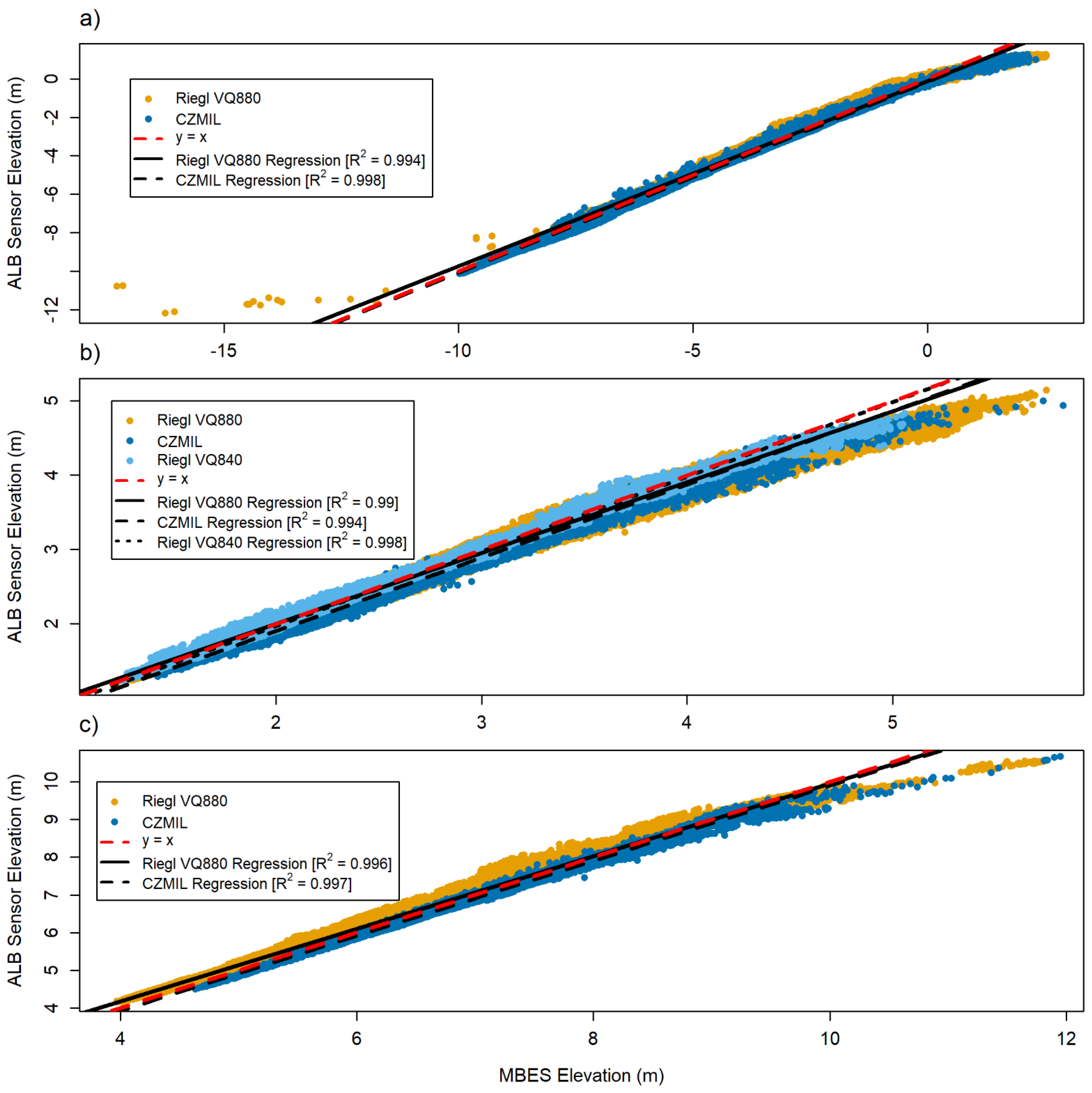
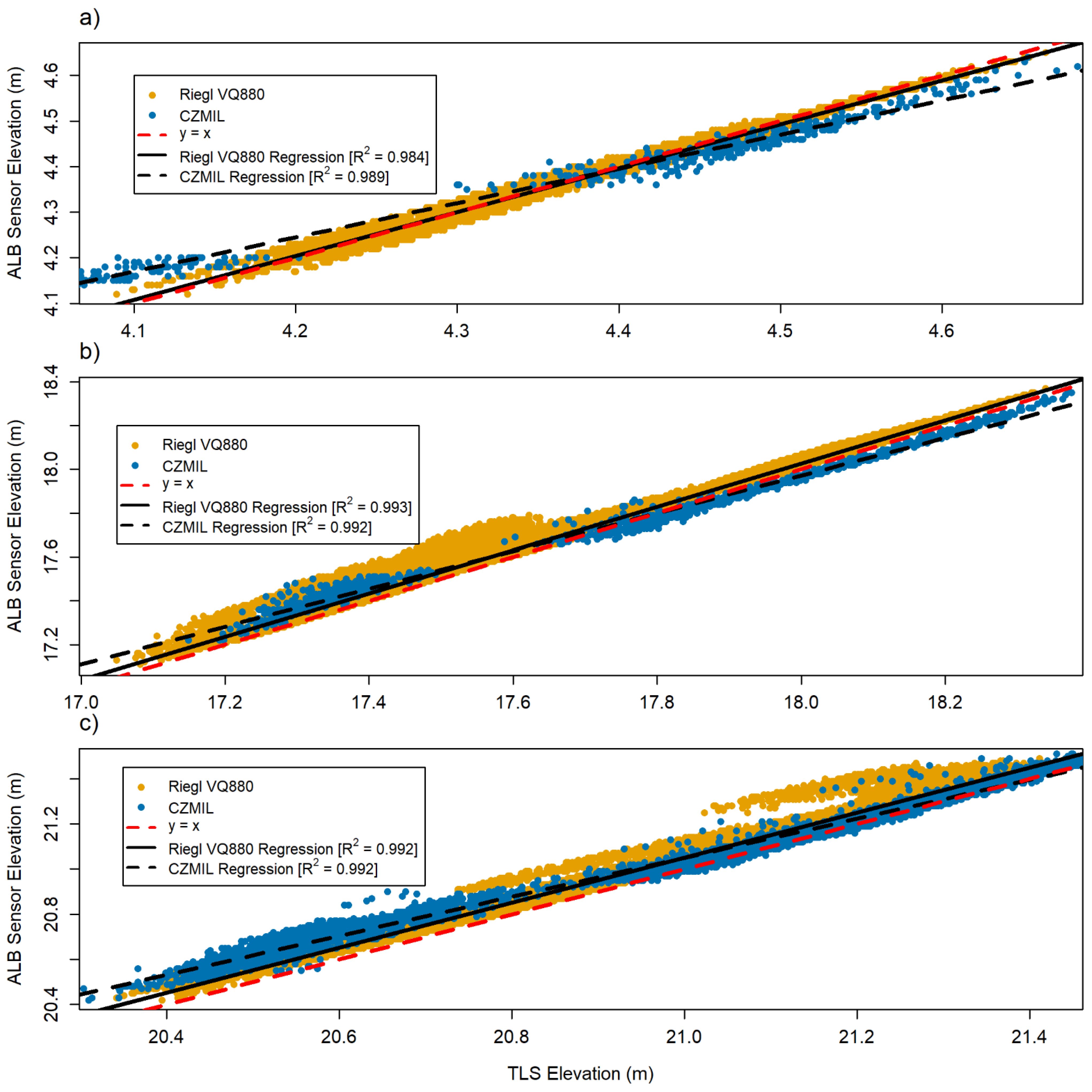
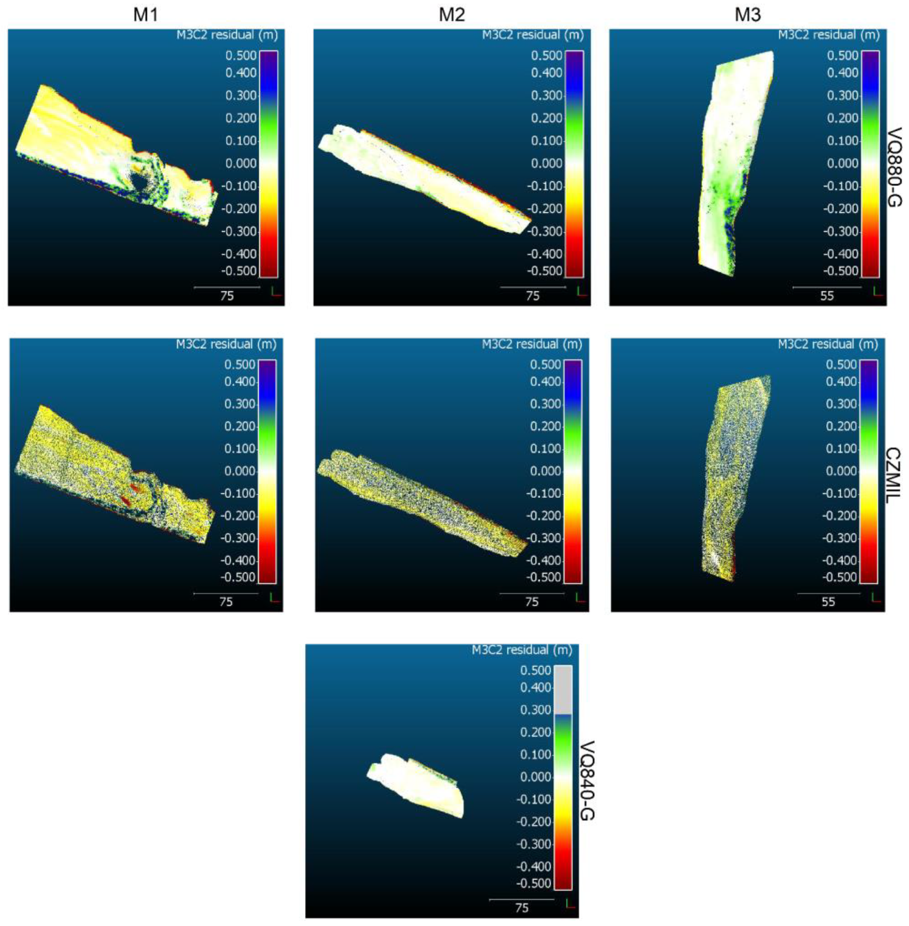
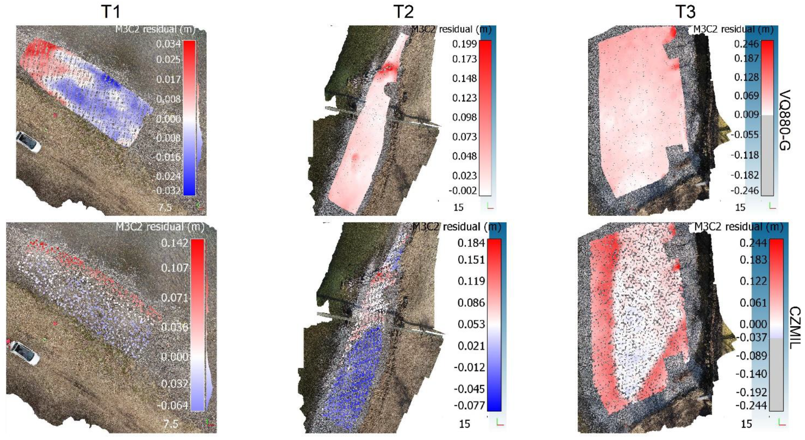
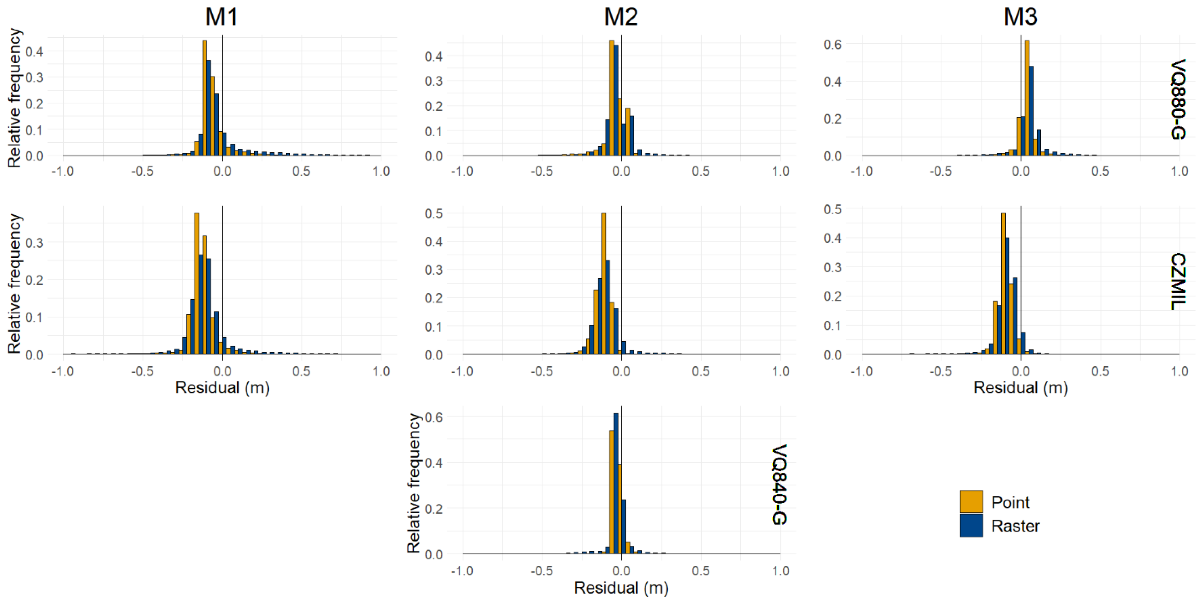
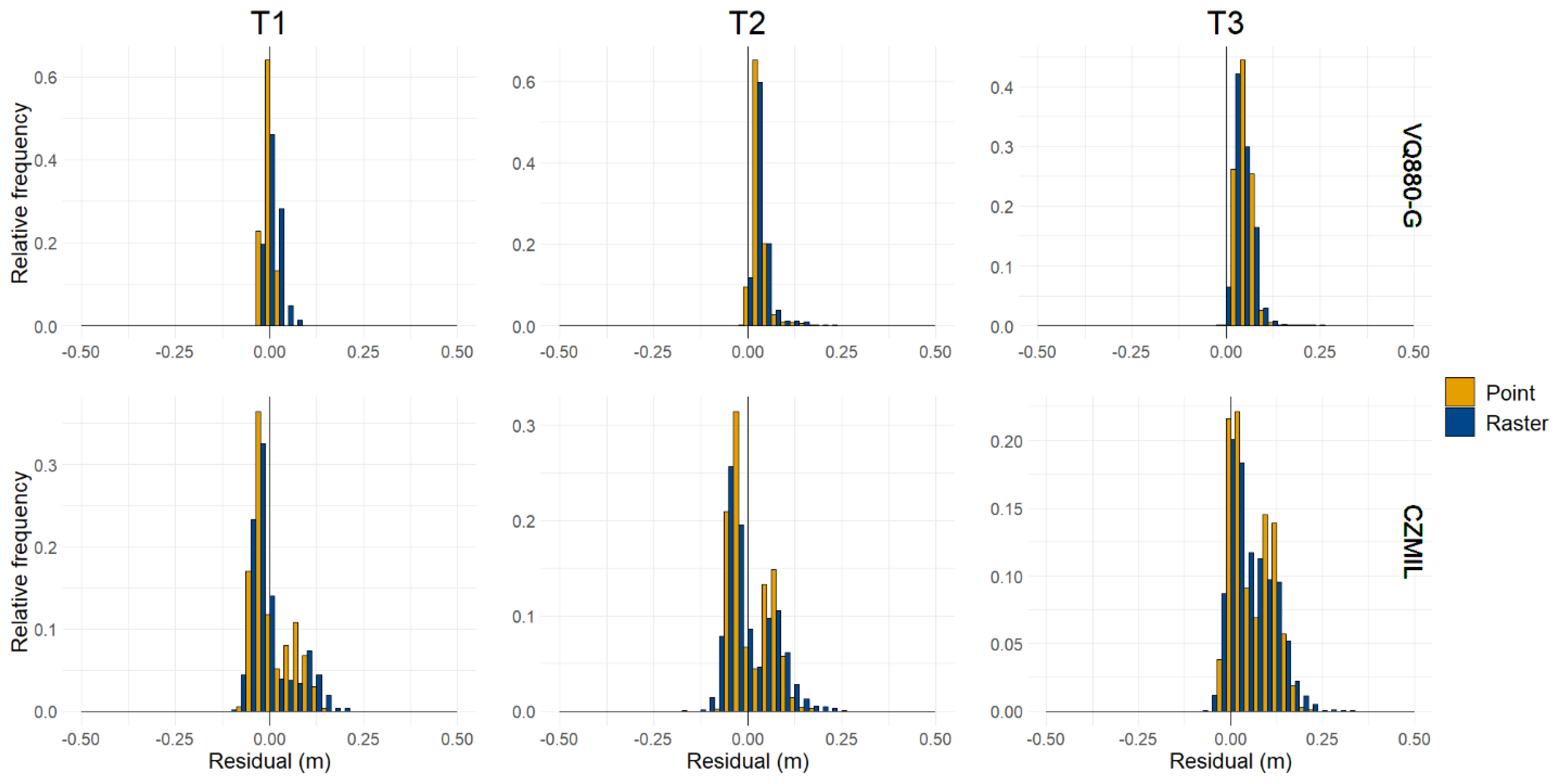
- Evaluate the differences in elevation between the bathymetric LiDAR point clouds and the MBES and TLS point clouds.
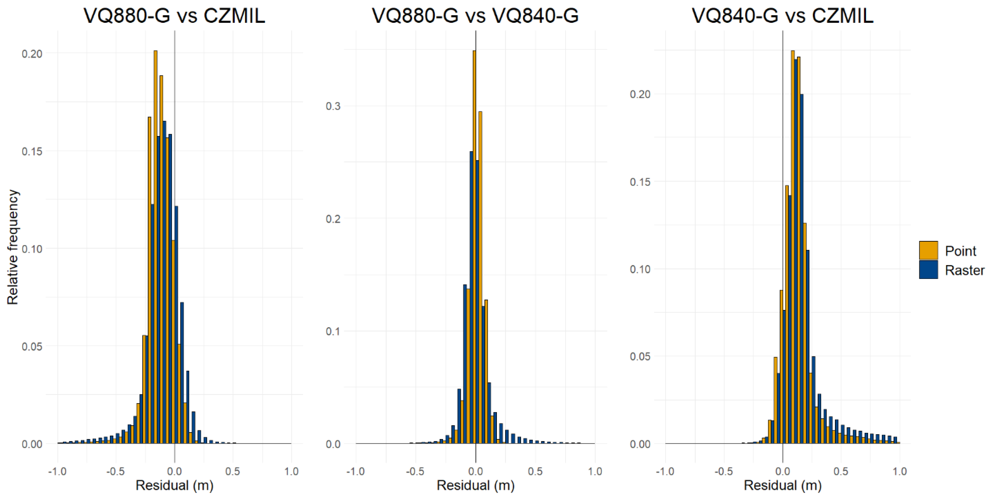
- Evaluate the differences in elevation of the bathymetric LiDAR point clouds against each other.
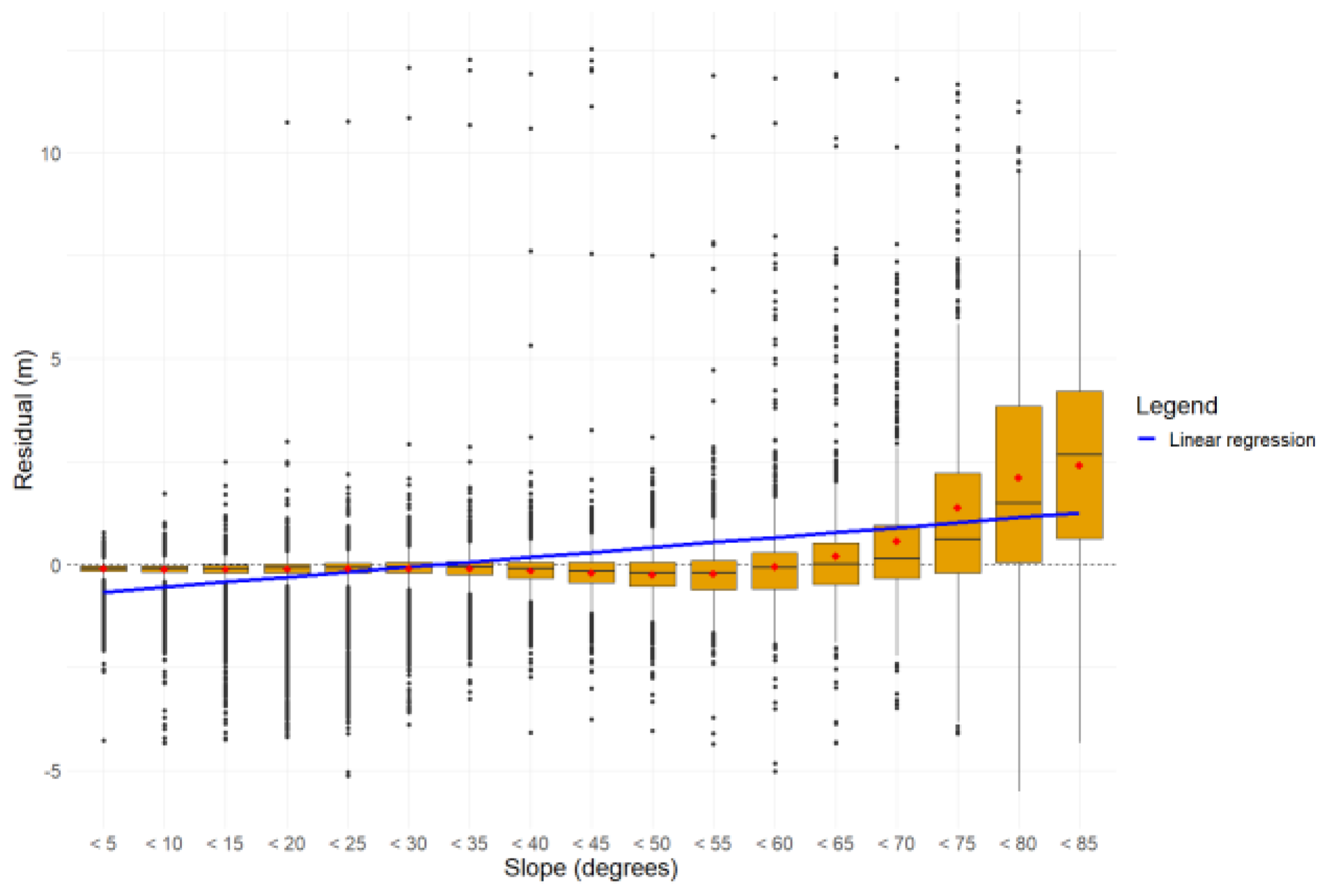
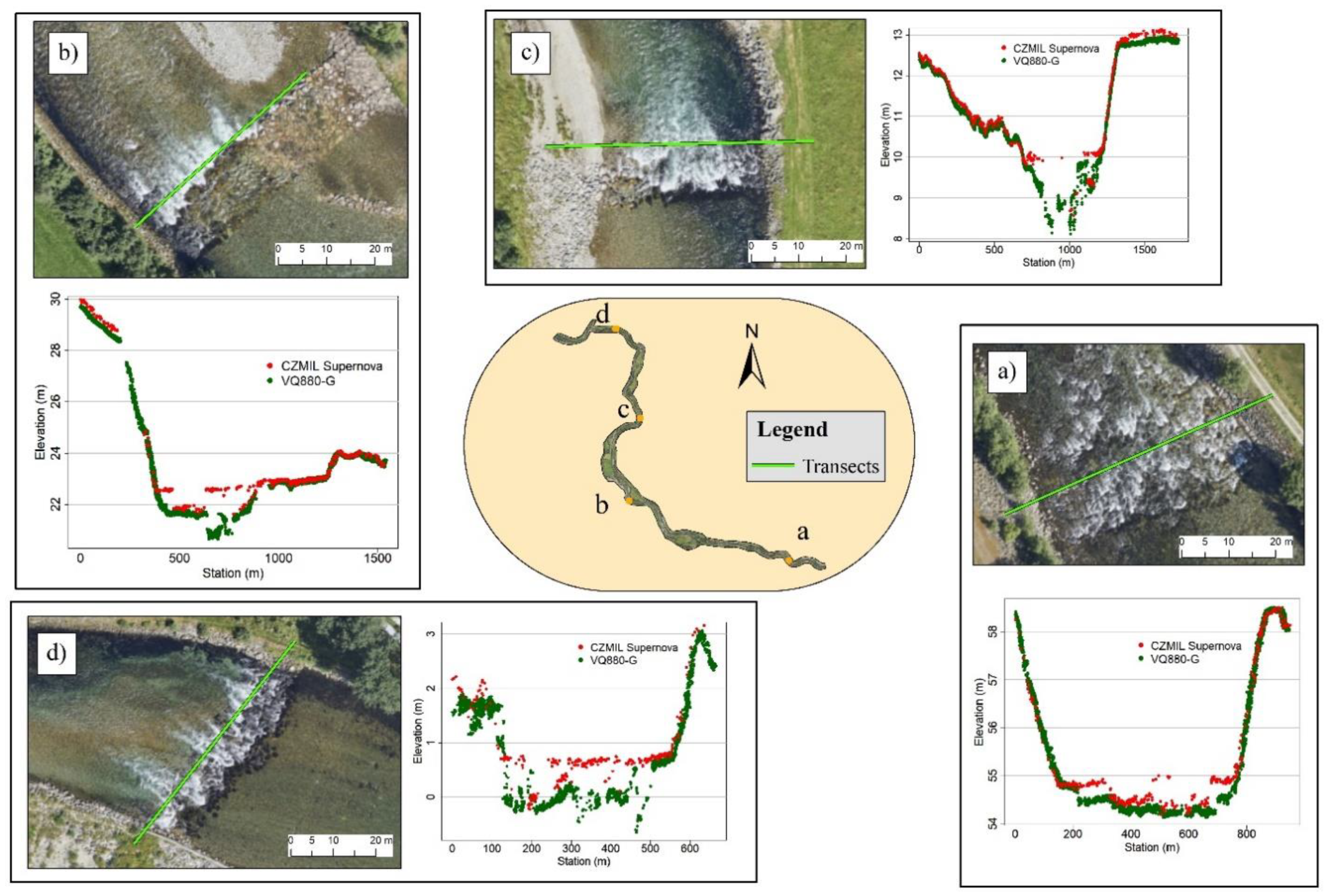
- Relating the differences to river features such as depth, steepness of banks, abrupt elevation changes, and whitewater locations.
2. Data
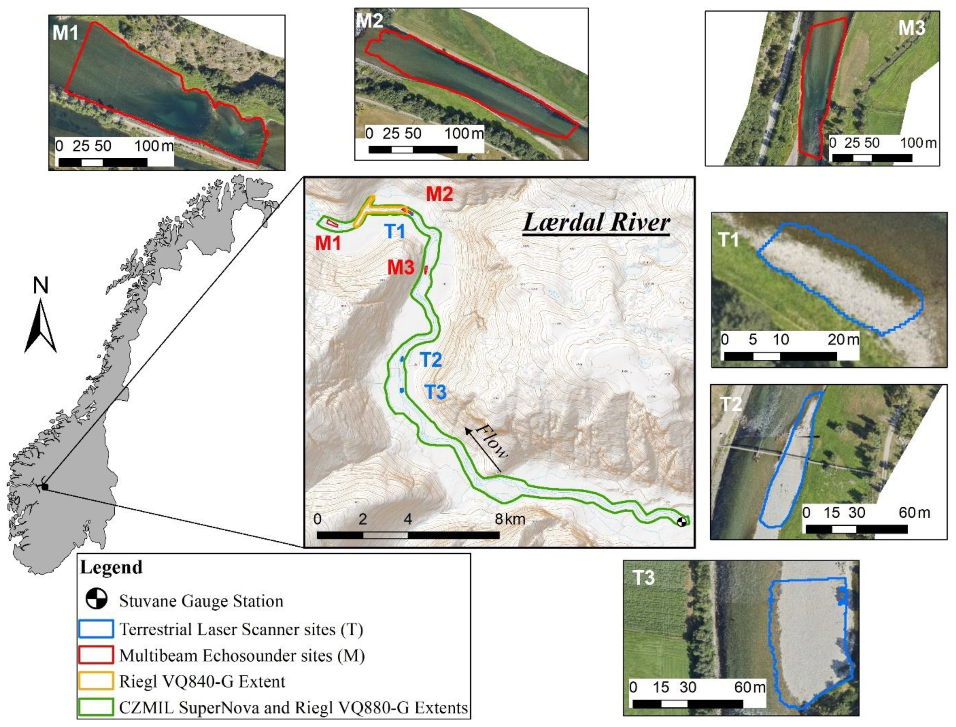
2.1. Study Site
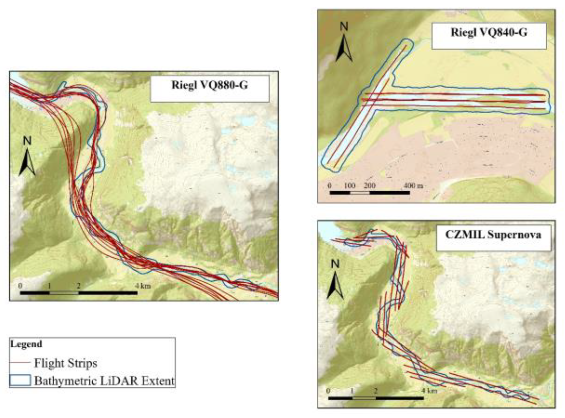
2.2. Bathymetric LiDAR Data
2.3. MBES and TLS Datasets
3. Methodology
4. Results
5. Discussion
Author Contributions
Funding
Data Availability Statement
Conflicts of Interest
Appendix A

References
- Saleh, F.; Ducharne, A.; Flipo, N.; Oudin, L.; Ledoux, E. Impact of river bed morphology on discharge and water levels simulated by a 1D Saint–Venant hydraulic model at regional scale. J. Hydrol. 2013, 476, 169–177. [Google Scholar] [CrossRef]
- Cook, A.; Merwade, V. Effect of topographic data, geometric configuration and modeling approach on flood inundation mapping. J. Hydrol. 2009, 377, 131–142. [Google Scholar] [CrossRef]
- Kinzel, P.J.; Legleiter, C.J.; Nelson, J.M. Mapping River Bathymetry with a Small Footprint Green LiDAR: Applications and Challenges. J. Am. Water Resour. Assoc. 2013, 49, 183–204. [Google Scholar] [CrossRef]
- Winterbottom, S.J.; Gilvear, D.J. Quantification of channel bed morphology in gravel-bed rivers using airborne multispectral imagery and aerial photography. Regul. Rivers Res. Manag. 1997, 13, 489–499. [Google Scholar] [CrossRef]
- Allouis, T.; Bailly, J.-S.; Pastol, Y.; Le Roux, C. Comparison of LiDAR waveform processing methods for very shallow water bathymetry using Raman, near-infrared and green signals. Earth Surf. Process. Landf. 2010, 35, 640–650. [Google Scholar] [CrossRef]
- Bangen, S.G.; Wheaton, J.M.; Bouwes, N.; Bouwes, B.; Jordan, C. A methodological intercomparison of topographic survey techniques for characterizing wadeable streams and rivers. Geomorphology 2014, 206, 343–361. [Google Scholar] [CrossRef]
- Hostache, R.; Matgen, P.; Giustarini, L.; Teferle, F.N.; Tailliez, C.; Iffly, J.-F.; Corato, G. A drifting GPS buoy for retrieving effective riverbed bathymetry. J. Hydrol. 2015, 520, 397–406. [Google Scholar] [CrossRef] [Green Version]
- Dey, S.; Saksena, S.; Merwade, V. Assessing the effect of different bathymetric models on hydraulic simulation of rivers in data sparse regions. J. Hydrol. 2019, 575, 838–851. [Google Scholar] [CrossRef]
- Casas, A.; Benito, G.; Thorndycraft, V.R.; Rico, M. The topographic data source of digital terrain models as a key element in the accuracy of hydraulic flood modelling. Earth Surf. Process. Landf. 2006, 31, 444–456. [Google Scholar] [CrossRef]
- McKean, J.; Nagel, D.; Tonina, D.; Bailey, P.; Wright, C.W.; Bohn, C.; Nayegandhi, A. Remote Sensing of Channels and Riparian Zones with a Narrow-Beam Aquatic-Terrestrial LIDAR. Remote Sens. 2009, 1, 1065–1096. [Google Scholar] [CrossRef]
- McKean, J.; Tonina, D.; Bohn, C.; Wright, C.W. Effects of bathymetric lidar errors on flow properties predicted with a multi-dimensional hydraulic model. J. Geophys. Res. Earth Surf. 2014, 119, 644–664. [Google Scholar] [CrossRef]
- Gao, J. Bathymetric mapping by means of remote sensing: Methods, accuracy and limitations. Prog. Phys. Geogr. 2009, 33, 103–116. [Google Scholar] [CrossRef]
- Hilldale, R.C.; Raff, D. Assessing the ability of airborne LiDAR to map river bathymetry. Earth Surf. Process. Landf. 2008, 33, 773–783. [Google Scholar] [CrossRef]
- Legleiter, C.J.; Harrison, L.R. Remote Sensing of River Bathymetry: Evaluating a Range of Sensors, Platforms, and Algorithms on the Upper Sacramento River, California, USA. Water Resour. Res. 2019, 55, 2142–2169. [Google Scholar] [CrossRef]
- Lefsky, M.A.; Cohen, W.B.; Parker, G.G.; Harding, D.J. Lidar remote sensing for ecosystem studies. Bioscience 2002, 52, 19–30. [Google Scholar] [CrossRef]
- LaRocque, P.E.; West, G.R. Airborne Laser Hydrography: An Introduction. 1999. Available online: https://www.researchgate.net/profile/Paul-Larocque-2/publication/228867617_Airborne_laser_hydrography_an_introduction/links/544141ef0cf2e6f0c0f607c0/Airborne-laser-hydrography-an-introduction.pdf (accessed on 15 June 2022).
- Juárez, A.; Adeva-Bustos, A.; Alfredsen, K.; Dønnum, B.O. Performance of A Two-Dimensional Hydraulic Model for the Evaluation of Stranding Areas and Characterization of Rapid Fluctuations in Hydropeaking Rivers. Water 2019, 11, 201. [Google Scholar] [CrossRef] [Green Version]
- Moniz, P.J.; Pasternack, G.B.; Massa, D.A.; Stearman, L.W.; Bratovich, P.M. Do rearing salmonids predictably occupy physical microhabitat? J. Ecohydraulics 2020, 5, 132–150. [Google Scholar] [CrossRef]
- Saltveit, S.J.; Brabrand, Å.; Juárez, A.; Stickler, M.; Dønnum, B.O. The Impact of Hydropeaking on Juvenile Brown Trout (Salmo trutta) in a Norwegian Regulated River. Sustainability 2020, 12, 8670. [Google Scholar] [CrossRef]
- Lague, D.; Feldmann, B. Chapter 2—Topo-bathymetric airborne LiDAR for fluvial-geomorphology analysis. In Remote Sensing of Geomorphology; Tarolli, P., Mudd, S.M., Eds.; Developments in Earth Surface Processes; Elsevier: Amsterdam, The Netherlands, 2020; Volume 23, pp. 25–54. [Google Scholar]
- Mandlburger, G.; Hauer, C.; Wieser, M.; Pfeifer, N. Topo-Bathymetric LiDAR for Monitoring River Morphodynamics and Instream Habitats-A Case Study at the Pielach River. Remote Sens. 2015, 7, 6160–6195. [Google Scholar] [CrossRef] [Green Version]
- Awadallah, M.O.M.; Juárez, A.; Alfredsen, K. Comparison between Topographic and Bathymetric LiDAR Terrain Models in Flood Inundation Estimations. Remote Sens. 2022, 14, 227. [Google Scholar] [CrossRef]
- Juárez, A.; Alfredsen, K.; Stickler, M.; Adeva-Bustos, A.; Suárez, R.; Seguín-García, S.; Hansen, B. A Conflict between Traditional Flood Measures and Maintaining River Ecosystems? A Case Study Based upon the River Lærdal, Norway. Water 2021, 13, 1884. [Google Scholar] [CrossRef]
- Quadros, N. Unlocking the characteristics of bathymetric LiDAR sensors. LiDAR Magazine, 3 December 2013; 62–67. [Google Scholar]
- Feygels, V.; Ramnath, V.; Marthouse, R.; Aitken, J.; Smith, B.; Clark, N.; Renz, E.; Duong, H.; Wozencraft, J.; Reisser, J. CZMIL as a rapid environmental disaster response tool. In Proceedings of the OCEANS 2017—Aberdeen, Aberdeen, UK, 19–22 June 2017; 2017; Volume 2017, pp. 1–7. [Google Scholar]
- Ramnath, V.; Feygels, V.; Kalluri, H.; Smith, B. CZMIL (Coastal Zone Mapping and Imaging Lidar) bathymetric performance in diverse littoral zones. In Proceedings of the OCEANS 2015—MTS/IEEE Washington, Washington, DC, USA, 19–22 October 2015. [Google Scholar] [CrossRef]
- Wozencraft, J.M. Requirements for the Coastal Zone Mapping and Imaging Lidar (CZMIL). In Proceedings of the SPIE—The International Society for Optical Engineering, Orlando, FL, USA, 12 May 2010; Volume 7695. [Google Scholar]
- Costa, B.M.; Battista, T.A.; Pittman, S.J. Comparative evaluation of airborne LiDAR and ship-based multibeam SoNAR bathymetry and intensity for mapping coral reef ecosystems. Remote Sens. Environ. 2009, 113, 1082–1100. [Google Scholar] [CrossRef]
- Riegl Riegl VQ-880-NG data sheet. 2016. Available online: http://www.riegl.com/uploads/tx_pxpriegldownloads/RIEGL_VQ-880-G_Datasheet_2018-09-28.pdf (accessed on 15 June 2022).
- Mandlburger, G.; Pfennigbauer, M.; Schwarz, R.; Flöry, S.; Nussbaumer, L. Concept and Performance Evaluation of a Novel. Remote Sens. 2020, 12, 28. [Google Scholar] [CrossRef] [Green Version]
- Pfennigbauer, M.; Rieger, P.; Schwarz, R.; Ullrich, A. Impact of beam parameters on the performance of a topo-bathymetric lidar sensor. In Proceedings of the Laser Radar Technology and Applications XXVII, Orlando, FL, USA, 3 June 2022; Volume 12110, pp. 107–117. [Google Scholar] [CrossRef]
- Wang, D.; Xing, S.; He, Y.; Yu, J.; Xu, Q.; Li, P. Evaluation of a New Lightweight UAV-Borne Topo-Bathymetric LiDAR for Shallow Water Bathymetry and Object Detection. Sensors 2022, 22, 1379. [Google Scholar] [CrossRef] [PubMed]
- Fernandez-Diaz, J.C.; Glennie, C.L.; Carter, W.E.; Shrestha, R.L.; Sartori, M.P.; Singhania, A.; Legleiter, C.J.; Overstreet, B.T. Early Results of Simultaneous Terrain and Shallow Water Bathymetry Mapping Using a Single-Wavelength Airborne LiDAR Sensor. IEEE J. Sel. Top. Appl. Earth Obs. Remote Sens. 2014, 7, 623–635. [Google Scholar] [CrossRef]
- Kinzel, P.J.; Wright, C.W.; Nelson, J.M.; Burman, A.R. Evaluation of an Experimental LiDAR for Surveying a Shallow, Braided, Sand-Bedded River. J. Hydraul. Eng. 2007, 133, 838–842. [Google Scholar] [CrossRef] [Green Version]
- Tonina, D.; McKean, J.A.; Benjankar, R.M.; Wright, C.W.; Goode, J.R.; Chen, Q.; Reeder, W.J.; Carmichael, R.A.; Edmondson, M.R. Mapping river bathymetries: Evaluating topobathymetric LiDAR survey. Earth Surf. Process. Landf. 2019, 44, 507–520. [Google Scholar] [CrossRef]
- Legleiter, C.J.; Overstreet, B.T.; Glennie, C.L.; Pan, Z.; Fernandez-Diaz, J.C.; Singhania, A. Evaluating the capabilities of the CASI hyperspectral imaging system and Aquarius bathymetric LiDAR for measuring channel morphology in two distinct river environments. Earth Surf. Process. Landf. 2016, 41, 344–363. [Google Scholar] [CrossRef]
- Yoshida, K.; Maeno, S.; Ogawa, S.; Mano, K.; Nigo, S. Estimation of distributed flow resistance in vegetated rivers using airborne topo-bathymetric LiDAR and its application to risk management tasks for Asahi River flooding. J. Flood Risk Manag. 2020, 13, e12584. [Google Scholar] [CrossRef]
- Yoshida, K.; Kajikawa, Y.; Nishiyama, S.; Islam, M.T.; Adachi, S.; Sakai, K. Three-dimensional numerical modelling of floods in river corridor with complex vegetation quantified using airborne LiDAR imagery. J. Hydraul. Res. 2022, 1–21. [Google Scholar] [CrossRef]
- Miller, P.; Addy, S. Topo-Bathymetric Lidar in Support of Hydromorphological Assessment, River Restoration and Flood Risk Management. CREW Report, 13 May 2019; 1–41. [Google Scholar]
- Kinzel, P.J.; Legleiter, C.J.; Grams, P.E. Field evaluation of a compact, polarizing topo-bathymetric lidar across a range of river conditions. River Res. Appl. 2021, 37, 531–543. [Google Scholar] [CrossRef]
- Islam, M.T.; Yoshida, K.; Nishiyama, S.; Sakai, K.; Tsuda, T. Characterizing vegetated rivers using novel unmanned aerial vehicle-borne topo-bathymetric green lidar: Seasonal applications and challenges. River Res. Appl. 2022, 38, 44–58. [Google Scholar] [CrossRef]
- Mandlburger, G. A review of airborne laser bathymetry for mapping of inland and coastal waters. Hydrogr. Nachr. 2020, 6–15. [Google Scholar] [CrossRef]
- Gottschalk, L.; Jensen, L.J.; Lundquist, D.; Solantie, R.; Tollan, A. Hydrologic regions in the Nordic countries. Nord. Hydrol. 1979, 10, 273–286. [Google Scholar] [CrossRef]
- Alfredsen, K.; Awadallah, M.O.M. Vurdering av Hydraulisk Effekt av Tersklar i Lærdalselva; NTNU: Trondheim, Norway, 2022. [Google Scholar]
- Skår, B.; Gabrielsen, S.E.; Stranzl, S. Habitatkartlegging av Lærdalselva fra Voll bru til sjø Laboratorium for Ferskvannsøkologi og Innlandsfiske; NORCE: Bergen, Norway, 2017. [Google Scholar]
- Statens Kartverk. Produksjon av Basis Geodata—Standarder Geografisk Informasjon. Version 1.0. 2015, pp. 1–94. Available online: https://www.kartverket.no/globalassets/geodataarbeid/standardisering/standarder/standarder-geografisk-informasjon/produksjon-av-basis-geodata-1.0-standarder-geografisk-informasjon.pdf (accessed on 15 June 2022).
- Kartverket. Produktspesifikasjon Nasjonal Modell for Høydedata fra Laserskanning (FKB-Laser). No. Version 2.0, Norwegian Mapping Authorities. 2013, pp. 1–27. Available online: https://register.geonorge.no/data/documents/Produktspesifikasjoner_FKB-Laser_v1_fkb-laser-v30-2018-01-01_.pdf (accessed on 15 June 2022).
- Glira, P.; Pfeifer, N.; Mandlburger, G. Rigorous strip adjustment of UAV-based laserscanning data including time-dependent correction of trajectory errors. Photogramm. Eng. Remote Sens. 2016, 82, 945–954. [Google Scholar] [CrossRef] [Green Version]
- Applanix. POS MV OceanMaster. 2019. Available online: https://www.applanix.com/downloads/products/specs/posmv/POS-MV-OceanMaster.pdf (accessed on 10 July 2022).
- Norbit. NORBIT WINGHEAD i77h. 2020. Available online: https://norbit.com/media/PS-200004-4_WINGHEAD-i77h_A4.pdf (accessed on 10 July 2022).
- Leica-Geosystems. Leica ScanStation P50. 2017. Available online: https://leica-geosystems.com/products/laser-scanners/scanners/leica-scanstation-p50 (accessed on 10 July 2022).
- CloudCompare. CloudCompare (Version 2.11.3) [GPL Software]. 2020. Available online: http://www.cloudcompare.org/ (accessed on 1 March 2022).
- Lague, D.; Brodu, N.; Leroux, J. Accurate 3D comparison of complex topography with terrestrial laser scanner: Application to the Rangitikei canyon (N-Z). ISPRS J. Photogramm. Remote Sens. 2013, 82, 10–26. [Google Scholar] [CrossRef] [Green Version]
- Brasington, J.; Langham, J.; Rumsby, B. Methodological sensitivity of morphometric estimates of coarse fluvial sediment transport. Geomorphology 2003, 53, 299–316. [Google Scholar] [CrossRef]
- Lallias-Tacon, S.; Liébault, F.; Piégay, H. Step by step error assessment in braided river sediment budget using airborne LiDAR data. Geomorphology 2014, 214, 307–323. [Google Scholar] [CrossRef]
- Weber, M.D.; Pasternack, G.B. Valley-scale morphology drives differences in fluvial sediment budgets and incision rates during contrasting flow regimes. Geomorphology 2017, 288, 39–51. [Google Scholar] [CrossRef] [Green Version]
- Wheaton, J.M.; Brasington, J.; Darby, S.E.; Sear, D.A. Accounting for uncertainty in DEMs from repeat topographic surveys: Improved sediment budgets. Earth Surf. Process. Landf. 2010, 35, 136–156. [Google Scholar] [CrossRef]
- Antonarakis, A.S.; Richards, K.S.; Brasington, J. Object-based land cover classification using airborne LiDAR. Remote Sens. Environ. 2008, 112, 2988–2998. [Google Scholar] [CrossRef]
- Crosilla, F.; Macorig, D.; Scaioni, M.; Sebastianutti, I.; Visintini, D. LiDAR data filtering and classification by skewness and kurtosis iterative analysis of multiple point cloud data categories. Appl. Geomat. 2013, 5, 225–240. [Google Scholar] [CrossRef] [Green Version]
- Bulmer, M.G. Principles of Statistics; Dover Books: New York, NY, USA, 1979. [Google Scholar]
- Glira, P.; Pfeifer, N.; Briese, C.; Ressl, C. A Correspondence Framework for ALS Strip Adjustments based on Variants of the ICP Algorithm. Photogramm. Fernerkund. Geoinf. 2015, 2015, 275–289. [Google Scholar] [CrossRef]
- Skinner, K.D. Evaluation of LiDAR-Acquired Bathymetric and Topographic Data Accuracy in Various Hydrogeomorphic Settings in the Deadwood and South Fork Boise Rivers, West-Central Idaho, 2007; U.S. Geological Survey Scientific Investigations Report 2011–5051; U.S. Department of the Interior: Washington, DC, USA, 2011. [Google Scholar]


| CZMIL Supernova | Riegl VQ880-G | Riegl VQ840-G | |
|---|---|---|---|
| Sensor short name | CZMIL | VQ880 | VQ840 |
| Sensor type | Topo-Shallow Bathy (1) | Topo-Bathy | Topo-Bathy |
| Weight (kg) | 270 | 65 | 12 |
| Dimensions (cm) | 89 × 60 × 90—sensor head 59 × 56.5 × 106—operation rack | 52 × 52 × 69 | 36 × 29 × 20 |
| Laser Channels (nm) | 532/532/1064 | 532 | 532 |
| Camera | Phase One iXM-RS150F | RGB | RGB |
| Measurement rate (kHz) | 180 | up to 550 kHz | 50–200 |
| Pulse Energy (mJ) | 1.75 | - | - |
| Pulse Duration (ns) | 1.57 | 1.5 | 1.5 |
| Field of view (deg) | ±20 | ±20 | ±20 |
| Beam divergence (mrad) | 1.9 | 0.7–1.1 | 1–6 |
| Input optics diameter (mm) | 200 | ||
| Nominal flying altitude (m) | 400–600 | 400 | 50–150 |
| Laser footprint (cm) | 75–112 | 50 @ 1.1mrad | 5 to 90 |
| Scan pattern | circular | circular | elliptical |
| Depth performance @ 15% Bottom Reflectance (Secchi depth) | 2 | 1.5 | 2 |
| Acquisition Date | 21 July 2021 | 26 September 2021 | 25 September 2021 |
| Discharge (m3/s) | 20 | 15 | 15 |
| Flight Height (m AGL) | ~400 | ~400 | ~95 |
| Laser footprint (cm) | 75 | 40 | 21 |
| Flight Lines excluding turns (km) | 45.3 | 332.3 | 9.1 |
| Coverage Topo-Bathy (km2) | 3.6 | 3.6 | 0.2 |
| Efficiency Topo-Bathy (km / km2) | 12.7 | 93.2 | 54.8 |
| Requested Density Bathy (point/m2) | 5 | 5 | 5 |
| Actual Density Bathy (point/m2) | 6 | 91 | 40 |
| Location | Comparison Scenario | Median (1) | RMS | Acceptance Percentage(2) | Acceptance Limit | |||
|---|---|---|---|---|---|---|---|---|
| DEM | M3C2 | DEM | M3C2 | |||||
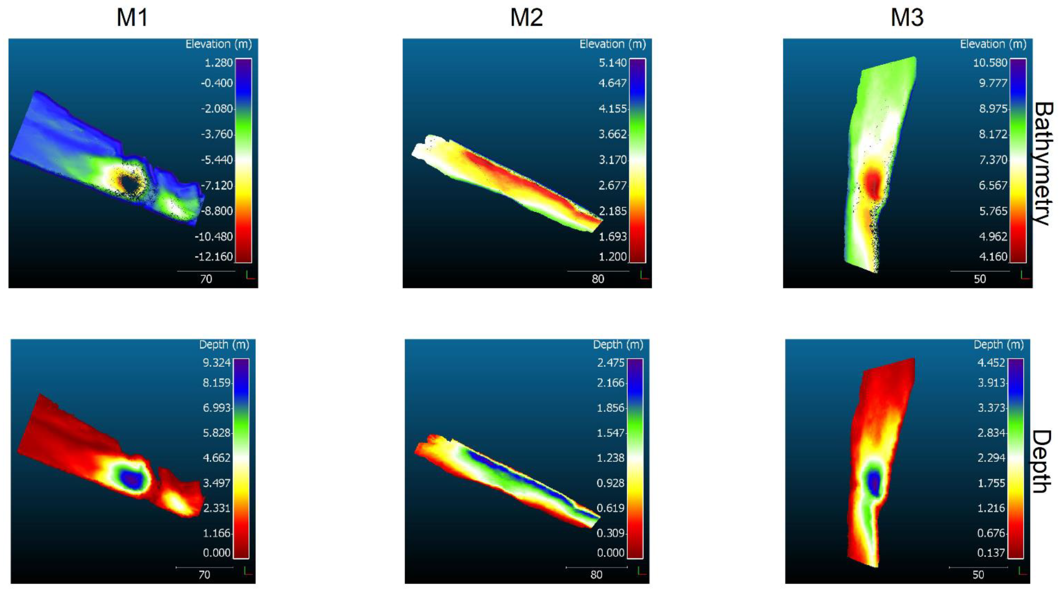
| MBES vs. ALB | M1 | MBES vs. Riegl VQ880 | −0.07 | −0.08 | 0.23 | 0.12 | 96 | ±0.20 |
| MBES vs. CZMIL | −0.13 | −0.13 | 0.22 | 0.15 | 94 | |||
| MBES vs. Riegl VQ840 (3) | NA | NA | NA | NA | NA | |||
| M2 | MBES vs. Riegl VQ880 | −0.05 | −0.03 | 0.11 | 0.08 | 97 | ||
| MBES vs. CZMIL | −0.11 | −0.11 | 0.15 | 0.12 | 96 | |||
| MBES vs. Riegl VQ840 (4) | −0.03 | −0.03 | 0.09 | 0.03 | 100 | |||
| M3 | MBES vs. Riegl VQ880 | 0.04 | 0.04 | 0.11 | 0.06 | 99 | ||
| MBES vs. CZMIL | −0.09 | −0.09 | 0.14 | 0.11 | 99 | |||
| MBES vs. Riegl VQ840 (3) | NA | NA | NA | NA | NA | |||
| TLS vs. ALB | T1 | TLS vs. Riegl VQ880 | 0.00 | −0.01 | 0.02 | 0.01 | 100 | ±0.10 |
| TLS vs. CZMIL | −0.02 | −0.02 | 0.06 | 0.05 | 94 | |||
| T2 | TLS vs. Riegl VQ880 | 0.03 | 0.03 | 0.04 | 0.04 | 98 | ||
| TLS vs. CZMIL | −0.02 | −0.02 | 0.06 | 0.05 | 96 | |||
| T3 | TLS vs. Riegl VQ880 | 0.04 | 0.05 | 0.05 | 0.06 | 99 | ||
| TLS vs. CZMIL | 0.04 | 0.04 | 0.08 | 0.08 | 71 | |||
| ALB vs. ALB | Full Reach | Riegl VQ880 vs. CZMIL | −0.10 | −0.12 | 0.21 | 0.16 | 82 | ±0.20 |
| VQ840 Extent | Riegl VQ840 vs. Riegl VQ880 | 0.02 | 0.02 | 0.13 | 0.07 | 99 | ||
| VQ840 Extent | Riegl VQ840 vs. CZMIL | 0.13 | 0.12 | 0.27 | 0.22 | 82 | ||
| Location | Comparison Scenario | Mean | Standard Deviation | Skewness | Kurtosis | |
|---|---|---|---|---|---|---|
| MBES vs. ALB | M1 | MBES vs. Riegl VQ880 | −0.06 | 0.10 | 1.01 | 67.82 |
| MBES vs. CZMIL | −0.12 | 0.09 | −0.73 | 22.06 | ||
| MBES vs. Riegl VQ840 (1) | NA | NA | NA | NA | ||
| M2 | MBES vs. Riegl VQ880 | −0.03 | 0.07 | −2.67 | 15.54 | |
| MBES vs. CZMIL | −0.11 | 0.05 | −1.54 | 13.51 | ||
| MBES vs. Riegl VQ840 (2) | −0.02 | 0.03 | 1.28 | 13.98 | ||
| M3 | MBES vs. Riegl VQ880 | 0.04 | 0.05 | −0.34 | 29.51 | |
| MBES vs. CZMIL | −0.09 | 0.05 | −2.82 | 47.21 | ||
| MBES vs. Riegl VQ840 (1) | NA | NA | NA | NA | ||
| TLS vs. ALB | T1 | TLS vs. Riegl VQ880 | 0.00 | 0.01 | 0.71 | 2.98 |
| TLS vs. CZMIL | 0.01 | 0.05 | 0.80 | 2.30 | ||
| T2 | TLS vs. Riegl VQ880 | 0.03 | 0.02 | 2.89 | 15.66 | |
| TLS vs. CZMIL | 0.01 | 0.05 | 0.60 | 2.07 | ||
| T3 | TLS vs. Riegl VQ880 | 0.05 | 0.02 | 1.77 | 11.48 | |
| TLS vs. CZMIL | 0.06 | 0.05 | 0.39 | 1.94 | ||
| ALB vs. ALB | Full Reach | Riegl VQ880 vs. CZMIL | −0.12 | 0.12 | −2.53 | 47.52 |
| VQ840 Extent | Riegl VQ840 vs. Riegl VQ880 | 0.02 | 0.07 | −2.61 | 68.78 | |
| VQ840 Extent | Riegl VQ840 vs. CZMIL | 0.14 | 0.17 | 4.01 | 114.13 |
Disclaimer/Publisher’s Note: The statements, opinions and data contained in all publications are solely those of the individual author(s) and contributor(s) and not of MDPI and/or the editor(s). MDPI and/or the editor(s) disclaim responsibility for any injury to people or property resulting from any ideas, methods, instructions or products referred to in the content. |
© 2023 by the authors. Licensee MDPI, Basel, Switzerland. This article is an open access article distributed under the terms and conditions of the Creative Commons Attribution (CC BY) license (https://creativecommons.org/licenses/by/4.0/).
Share and Cite
Awadallah, M.O.M.; Malmquist, C.; Stickler, M.; Alfredsen, K. Quantitative Evaluation of Bathymetric LiDAR Sensors and Acquisition Approaches in Lærdal River in Norway. Remote Sens. 2023, 15, 263. https://doi.org/10.3390/rs15010263
Awadallah MOM, Malmquist C, Stickler M, Alfredsen K. Quantitative Evaluation of Bathymetric LiDAR Sensors and Acquisition Approaches in Lærdal River in Norway. Remote Sensing. 2023; 15(1):263. https://doi.org/10.3390/rs15010263
Chicago/Turabian StyleAwadallah, Mahmoud Omer Mahmoud, Christian Malmquist, Morten Stickler, and Knut Alfredsen. 2023. "Quantitative Evaluation of Bathymetric LiDAR Sensors and Acquisition Approaches in Lærdal River in Norway" Remote Sensing 15, no. 1: 263. https://doi.org/10.3390/rs15010263