Article

On the Choice of the Most Suitable Period to Map Hill Lakes via Spectral Separability and Object-Based Image Analyses

Department of Engineering, Università degli Studi di Palermo, 90128 Palermo, Italy
Remote Sens. 2023, 15(1), 262; https://doi.org/10.3390/rs15010262
Submission received: 21 November 2022 / Revised: 27 December 2022 / Accepted: 29 December 2022 / Published: 2 January 2023
(This article belongs to the Special Issue Remote Sensing in Geomatics)

Abstract

:
Technological advances in Earth observation made images characterized by high spatial and temporal resolutions available, nevertheless bringing with them the radiometric heterogeneity of small geographical entities, often also changing in time. Among small geographical entities, hill lakes exhibit a widespread distribution, and their census is sometimes partial or shows unreliable data. High resolution and heterogeneity have boosted the development of geographic object-based image analysis algorithms. This research analyzes which is the most suitable period for acquiring satellite images to identify and delimitate hill lakes. This is achieved by analyzing the spectral separability of the surface reflectance of hill lakes from surrounding bare or vegetated soils and by implementing a semiautomatic procedure to enhance the segmentation phase of a GEOBIA algorithm. The proposed procedure was applied to high spatial resolution satellite images acquired in two different climate periods (arid and temperate), corresponding to dry and vegetative seasons. The segmentation parameters were tuned by minimizing an under- and oversegmentation metric on surfaces and perimeters of hill lakes selected as the reference. The separability of hill lakes from their surrounding was evaluated using Euclidean and divergence metrics both in the arid and temperate periods. The classification accuracy was evaluated by calculating the error matrix and normalized error matrix. Classes’ reflectances in the image acquired in the arid period show the highest average separability (3–4 higher than in the temperate one). The segmentation based on the reference areas performs more than that based on the reference perimeters (metric ≈ 20% lower). Both separability metrics and classification accuracies indicate that images acquired in the arid period are more suitable than temperate ones to map hill lakes.

1. Introduction

In recent years, the need for accurate classification procedures has led to the development of object-based image analysis (OBIA) algorithms, referred to as geographic OBIA (GEOBIA) if implemented to classify geographical entities. The object-based approach is based on the idea that the information required to classify an image does not belong only to a single pixel but to meaningful image objects and their mutual spatial relationships [1].
Blaschke [2] firstly, and Hossain and Chen [3] recently, presented the state of the art of GEOBIA techniques, emphasizing that these techniques increase the accuracy of the classification by synergistically using spectral and spatial information. GEOBIA, indeed, overcomes the so-called “salt and pepper” [4] effect on classification typical of pixel-based classification approaches. This result is obtained by delimitating spectrally homogeneous regions by image segmentation. Of course, segmentation procedures never produce purely homogeneous regions. However, the internal (within segment) heterogeneity is balanced with the external (between segments) heterogeneity. If compared with reference objects, automatic segmentation of an image produces over- and/or undersegmentation, thus only partially representing the reality. Optimizing the setup of segmentation algorithms is mandatory to improve classification accuracy.
A tailored segmentation is required to improve the accuracy of segments to match the real entities of the soil water vegetation system in the landscape. The soil water vegetation system, indeed, has an intrinsic complexity made up of interconnected and (sometimes) hardly distinguishable processes.
Indeed, resulting segments are generally regions generated by one or more homogeneity criteria through their spectral information. Recent algorithms’ solutions have emphasized how crucial spatial information is [5].
In the literature, many segmentation algorithms were implemented in open-source and commercial software, allowing one to retrieve homogeneous and semantically consistent groups of pixels. Not only is the pixels’ spectral information considered, but a combination of spectral and spatial information is as well [6]. Recently, a generic framework for combining multiple segmentations has been proposed [7]; the authors defined a segmentation confidence score allowing quantification of the local agreement between the different input segmentations. Johnson and Xie [8] used the variance and Local Moran’s index as a measure of local heterogeneity. Other authors, such as those from [9], introduced an automated approach to parameterizing multiscale image segmentation. In this research, a semiautomatic segmentation method was tested on hill lakes, since these are small enough to be seen by low-orbit satellites.
Many methods use Earth observation images for the lake delineation, including manual digitization, calculation of water indexes, hyperspectral indexes and methods based on classifications, including GEOBIA. Manual digitization ensures higher accuracy, although it is time-consuming and expensive [10]; water indexes (e.g., [11]) do not perform accurately when lakes and surrounding surfaces share similar spectral signatures such as hypertrophic water and dense vegetation in the wavelengths used for the calculation of the water indexes. Index algorithms have been successfully developed for hyperspectral images [12] including Short Wavelength Infrared, such as those acquired by the Hyperion hyperspectral instrument. However, hyperspectral satellite instruments currently do not provide high-spatial-resolution images. However, other authors developed quantitative methods for deriving water fractional cover from Short Wavelength Infrared satellite data based on the linear mixture theory [13].
The accuracy of GEOBIA, besides being influenced by the use of appropriate training samples, mainly depends on the segmentation efficacy [14].
Hill lakes (sometimes referred to in the literature as hilly lakes) often consist of small reservoirs playing an important role in the sustainable water management of agricultural areas [15]. Indeed, their presence reduces losses of agricultural land, reduces dam siltation, increases water table recharge and creates points for the development of irrigated cropping [16].
Several manuscripts faced the delimitation of large water bodies in geomatics research (e.g., [17,18,19]), while the extraction of hill lakes from satellite images has been under investigated due to their small size, despite their widespread spatial distribution, numerousness, and small size [20].
Nowadays, low-orbit satellites reach submeter or meter resolution [21,22], while in the study area, hill lakes have extensions ranging from 20 to 105 m2, with an average surface of 2 × 10³ m2 [23].
Besides the small surfaces, hill lakes are characterized by simple shapes that can be roughly described as squares or rectangles.
Despite the spatial resolution of low-orbit satellite images being suitable to see small entities, they bring with them the radiometric heterogeneity of the classes occurring in a study area (mostly bare and vegetated soils, besides water surfaces) [24].
To account for the seasonal spectral behavior of the abovementioned classes, the method was tested on two images out of two different periods: (i) a period when the water surface area is close to its maximum and surrounding vegetation cover is vigorous; (ii) another when the water surface area is at the minimum and surrounding plots are scarcely vegetated, sometimes dry, bare soils.
The paper is organized as follows. In Section 2, the materials and methods are presented. Specifically, in Section 2.1 and Section 2.2, the study area and the spectral and spatial characteristics of the selected satellite images are described. In Section 2.3, the methods, including the spectral separability and the segmentation procedure tailored to the object-based classification are briefly described. The results are presented and discussed in Section 3. In Section 4, the main findings of the study are briefly summarized, and indications of the most suitable time for acquiring satellite images to detect hill lakes are given. A list of the acronyms and symbols used in the manuscript is reported in the Appendix A.

2. Materials and Methods
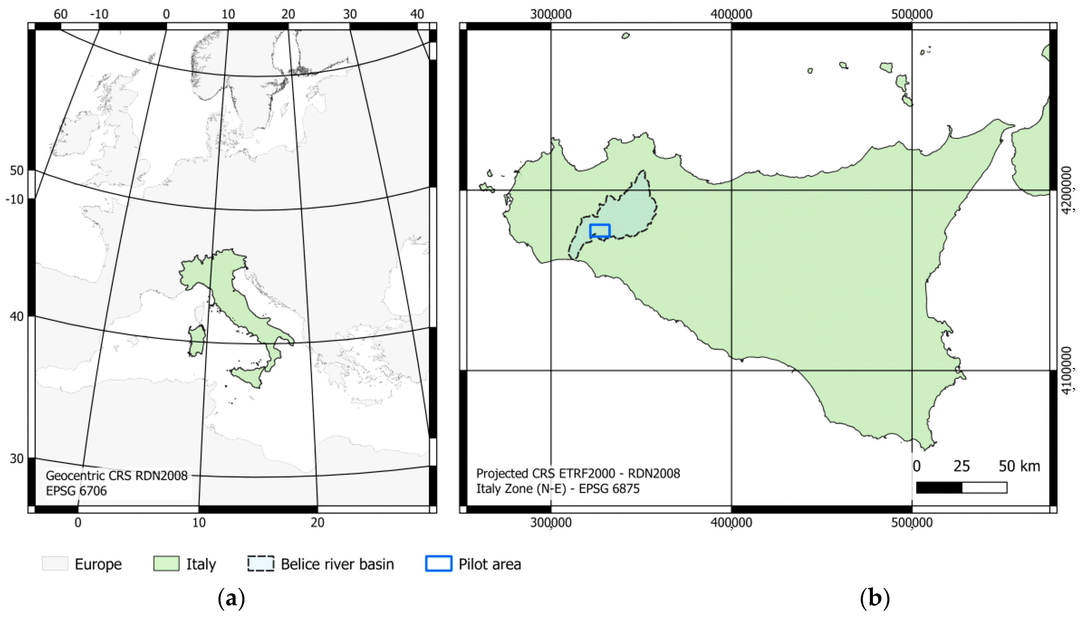
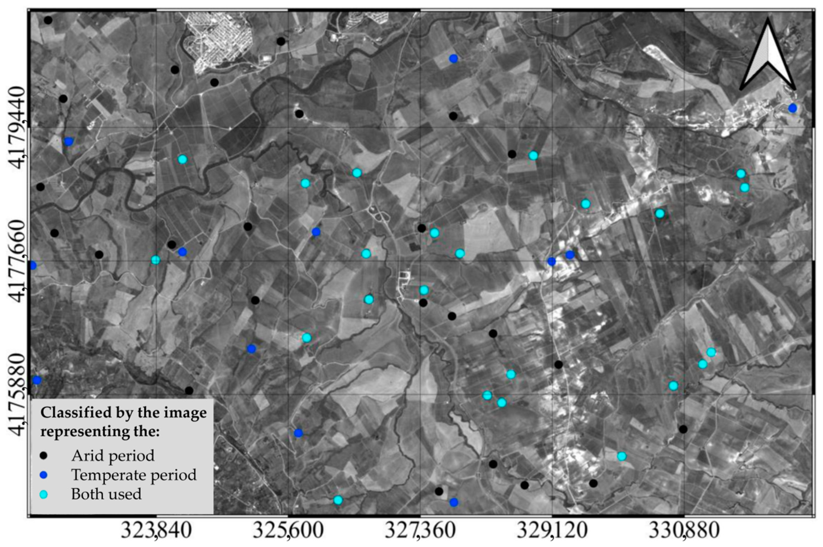
2.1. Study Area

The test area is located in western Sicily (Italy, Figure 1a). It is a subset of the Belice River Basin (blue rectangle, in Figure 1b) and has an extension of about 70 km2. The whole basin (panel b, black line) has an extension of 964 km2, and it is one of the largest catchments in Sicily. The catchment is prevalently covered by grasslands and pastures (≈47%).
A great number of hill lakes (mostly small reservoirs for agricultural water supply) are widespread in the basin. Their number and distribution were identified in high-spatial-resolution Google Earth images acquired on 11 June 2018. The implemented dataset is made of 797 (actual) reservoirs. The hydrographic network, like all the watercourses of Sicily, exhibits a typical torrential character, particularly in the upstream branches. Hydrophyte vegetation (mainly Rubus ulmifolius and Arundo donax) is associated with rivers and streams.
Besides the spectral variability of the soil water vegetation system characterizing most of the natural catchments, the Belice River Basin was chosen because recent surveys by the local water authority report that no hill lakes were built or dismissed in the 2015–2019 period [23]. While the Italian Committee for Large Dams, based on Earth Observation data in 1988 and a regional census in 2010, reports that small reservoirs have increased by 60 % in ~22 years, on the contrary, based on the Italian Environmental Data Yearbook (14th edition, 2016), small reservoirs should have decreased by ~23% in the 27 years from 1988 to 2015 [25].

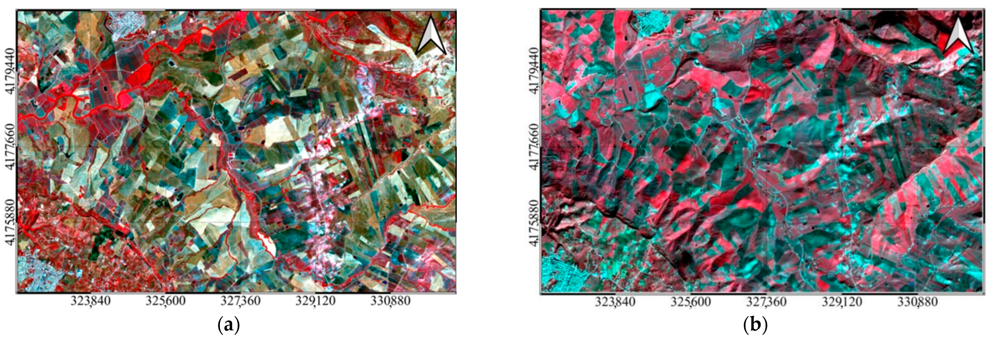
2.2. Satellite and Climate Data
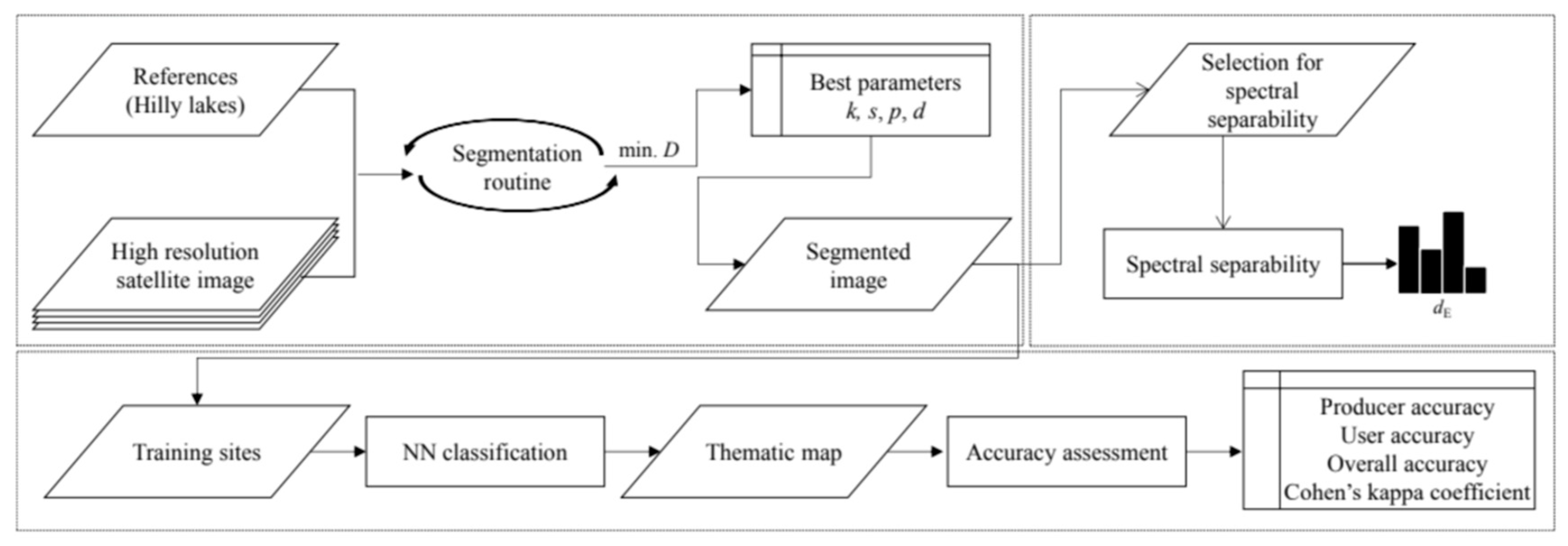
Two PlanetScope imageries were made available from Planet Labs Inc. (see portal https://www.planet.com, accessed on 25 December 2022) within the Planet’s Education and Research (E and R) Program. Images have a spatial resolution of 3 m and are composed of 4 spectral bands (VIS–NIR). PlanetScope images were selected over clear-sky days (0% cloud coverage).
The choice of the acquisition periods was based on the climatic characterization and the temporal behavior of the spatially averaged vegetation index over the study area since in different environments, accounting for climate and soil cover, the spectral separability of water bodies from surrounding entities and their classification accuracies are expected to change with seasons.
Within this research, a climatic characterization has been carried out by synthesizing thermo-pluviometric conditions through a Péguy climograph [26] as delivered in [27] by the Sicilian agro-meteorological information service (SIAS, Servizio Informativ Agrometereologico Siciliano) of the Sicilian regional government (Regione Siciliana) [28].
Based on the Péguy climograph calculated at the SIAS meteorological station of Sciacca (coordinates 4,162,344 North, 326,937 East, 56 m a.s.l), the area would be characterized by a temperate climate for 7 months a year (from October to April with a peak in January, while the remaining months shows an arid climate with the counterpart peak in August).
Regarding the temporal behavior of the vegetation cover, within this research, the time occurrence of maxima and minima were decided based on the Terra Moderate Resolution Imaging Spectroradiometer (MODIS) vegetation indexes (MOD13Q1, Version 6) product [29]. This product is generated every 16 days at 250 m spatial resolution as a Level 3 product. The MOD13Q1 product provides vegetation indexes, including the Normalized Difference Vegetation Index (NDVI), based on a compositing approach [30]. In particular, the algorithm chooses the best available pixel value from all the acquisitions from the 16 days based on the following criteria: low clouds, low view angle and the highest NDVI value. The temporal behavior of this product is accessible through the MODIS and VIIRS Land Products Global Subsetting and Visualization Tool [31].
Peaks of the vegetation index occur in different periods of the year depending on the year itself [32]; for instance: (a) in 2018, the maximum (NDVI averaged on the whole study area) was reached in March, while the minimum was reached in July; (b) in 2019, the maximum of the spatially averaged NDVI occurred in January and March, while the minimum occurred in August–September.
Considering both the climate characterization and the vegetation index temporal behavior, an image acquired on the 15 January 2019 was analyzed to represent the spectral characteristics of water surfaces and surrounding areas in the temperate period of the year, and an image acquired on 3 August 2019 was representative of the spectral characteristics in the arid period of the year. A color infrared (CIR) composite of the pilot areas (Figure 2) allows vegetation to be readily distinguishable in the image. Vegetation emerges in shades of red; soils vary from dark to light browns, and urban areas (sometimes bare soils as well) are cyan blue, depending on their composition; riparian vegetation appears bright red; hypertrophic water appears dark-reddish; oligotrophic water appears dark-bluish; turbid water appears cyan. Both bare and vegetated soils (mainly riparian vegetation) are shown in the arid period image (left panel, a), while a higher cover of vegetated soil is shown in the temperate period image (right panel, b).

2.3. Methods

To discuss the most appropriate season to select high spatial resolution satellite images to identify and correctly delimitate hilly lakes, the following procedure was implemented (see flowchart in Figure 3).
The segmentation routine is iterated to determine the best set of parameters minimizing both the under- and oversegmentation of satellite images acquired in different periods of the year. Several segments are selected: (i) to analyze the spectral separability among different classes; (ii) to run the classification procedure. The accuracy of the classification is assessed by calculating producer, user and overall accuracy, as well as Cohen’s kappa coefficient. Misclassified entities are analyzed to highlight whether the error is due to the segmentation or classification process.
The proposed procedure consists of three blocks: (i) firstly, the segmentation algorithm and the criteria to assess the parameters producing the best segmentation were chosen; (ii) then, the spectral separability between the entities chosen as a benchmark (hill lake class in this study case, mostly small agricultural reservoirs) and the others were analyzed; (iii) finally, once the images were classified, its accuracy was estimated as well as the spectral characteristics of the images, allowing one to discuss the performance of mapping the geographical entities.
Once the procedure was tested on pilot areas for both images acquired in the arid and temperate periods, it was applied and verified over the entire basin.

2.4. Segmentation

The key phase of the GEOBIA procedure is the tuning of the segmentation algorithm [3]. Some authors [33] provided a review of image segmentation techniques limiting the analysis to optical remote sensing. Indeed, compared to optical images, radar image segmentation techniques [34,35] still represent a challenging task because of the presence of speckle noise. Different segmentation algorithms have been implemented and tested in recent years for water-body detection and delimitation [36,37,38,39,40,41,42,43]. Among these, the Felzenszwalb and Huttenlocher algorithm [44] is implemented within the scikit-image library and interfaced with the Python library, Remote Sensing and GIS software library (RSGISLib). Additionally, the segmentation algorithm proposed by Shepherd et al. [45] is already implemented in the RSGISLib library [46].
Within this research, the Shepherd et al. [45] segmentation algorithm was applied. As reported by the authors, it compares favorably in most assessment metrics with other well-known methods such as multiresolution segmentation [47] implemented in eCognition [48] or the commonly used mean-shift [49] implemented within the Orfeo toolbox [50] when applied to a typical rural landscape.
An advantage of the Shepherd et al. algorithm [45] is the presence of a threshold that prevents small water bodies that are spectrally distinct from their neighbors to be merged with other areas due to their size.
A procedure was implemented to tune the segmentation parameters by minimizing an under- and oversegmentation metric. The segmentation was tuned on surfaces and perimeters of hill lakes that are small enough to be seen by low-orbit satellites.
The following segmentation parameters were calibrated by applying an iterative procedure: the number of clusters, k; the subsampling of the image for the data used within the segmentation, s; the minimum number of pixels within a segment, p; the spectral distance threshold for joining the segments, d (symbols’ meaning and units are reported in the Appendix A).
To optimize the segmentation procedure, a segmentation quality metric (D) was minimized [51,52]. The combined metric D has the structure of the root mean square error, RMSE, and it minimizes the oversegmentation metric, OS, and the undersegmentation metric, US, according to the Equation (1) [53]:
D = (OS2 + US2)0.5,
where O S i = A R i A   ( R i S i ) A R i and U S i = A S i A   ( R i S i ) A S i .
The metric D was averaged over the whole reference dataset ( D = D ¯ i ) to assess the overall performance of a given quadruple of segmentation parameters.
The operation A   ( R j S i ) indicates the area of a spatial intersection between two polygon vector layers, specifically the overlap of the reference polygon and the segment (see “OpenGIS Implementation Specification for Geographic information—Simple feature access—Part 1: Common architecture”, https://www.ogc.org/standards/sfa, accessed on 13 November 2022).
The expression A R i A   ( R i S i ) indicates the area of a reference polygon underestimated by a segment, while the expression A S i A   ( R i S i ) indicates that the area of a reference polygon is overestimated by a segment [54]. A segment could be larger than a reference polygon on one side and smaller on another side of the same reference polygon, i.e., over- and undersegmentation could coexist.
The values of AR were calculated by manually digitizing lake boundaries and then assumed to be reference polygons; on the other hand, AS is calculated based on the segmentation algorithm. Segments were selected according to the Equalized Random Stratified sampling method [55], which selects segments that are randomly distributed within each class, where each class has the same number of segments. The most suitable segmentation is the one producing the higher overlap with the reference areas and the lower value of D. To find the best set of parameters corresponding to the minimum value of D, a domain reduction technique was applied [56], implemented and tested in a Python routine over the pilot areas.

2.5. Spectral Separability

The analysis of spectral separability is a fundamental step to understanding whether a class could be confused with other ones: specifically, the hill lakes with surrounding bare and/or vegetated soil.
Different distance metrics could be used, including the simple Euclidean spectral distances between their means, the divergence; the transformed divergence, and the Jeffries–Matusita distance [57,58].
Separability was computed on the bottom of atmosphere reflectance using normalization of the Euclidean distance formulation [59]. The normalized Euclidean distance, dE, was obtained by rationing the Euclidean distance to its maximum value resulting from the classes.
However, the Euclidean distance does not account for clusters distributions; thus, more sophisticated separability measures such as the divergence (dD) [57] can be used, accounting for multivariate Gaussian distributions between two classes (i and j) according to the following formulation (2) [60]:
d D = 1 2 t r C i C j × C i 1 C j 1 + 1 2 t r C i 1 C j 1 × μ i μ j × μ i μ j T ,
In Equation (2), i and j refer to two signatures (classes) being compared; Ci and Cj indicate their covariance matrices, respectively; tr is a trace function, i.e., the sum of the elements of the diagonal of a square matrix; and T indicates transposition function.
Both spectral separability metrics were evaluated for the arid and temperate periods in the pilot areas to highlight whether and to what extent segments selected to train the classification algorithm could produce classes that can be confused with each other.

2.6. Classification

Once the best set of segmentation parameters were determined, it was possible to classify both images representing the temperate and arid periods, thus evaluating the best performance in delimiting hill lakes in terms of classification accuracy.
A multitude of machine learning classifiers can be trained on the same reference data to accomplish comparable performances during a test phase [61].
Several supervised classifiers are implemented in the Python library scikit-learn [62], including the support vector machines’ supervised learning methods [63], the decision tree nonparametric supervised learning method [64] and neural network supervised classification models [65], among others, with different classification algorithms resulting in different classification performances. However, the purpose of the research is not strictly to compare the accuracy of a classification algorithm but to verify whether the choice of an input image acquired in one season rather than another influences the identification and delimitation of hilly lakes.
Among machine learning classifiers, the nearest neighbor classifier, NN [66], implemented in the Python library scikit-learn [62], was selected and embedded in the classification code.
The classifier was trained by choosing a number of segments to be representative of each class. The object inherits the class from the closest sample object in the training set. Then, the classification accuracy was tested by verifying a number n of reference segments of the total number of segments N to ensure a given level of precision error e [67,68] (3):
n = N / 1 + N × e 2
Take a Random Forest (RF) algorithm as a comparison [24,69]. It is a perturb-and-combine technique [70] specifically designed for trees, already implemented in the sklearn.ensemble module. The RF algorithm was also applied to the pilot areas just to verify if the user and producer classification accuracy upset the results of the NN classifier and if the resulting overall accuracy is remarkably different (presumably higher).
The goodness of the classification was finally evaluated by calculating: the producer’s accuracy, PA and the user’s accuracy, UA, for each class; as well as the overall accuracy, OA [71] and Cohen’s kappa coefficient, K [72,73]. The classification metrics were evaluated for the pilot area and the whole basin.
Some authors [74,75] advocate normalizing error matrices to homogeneous margins to allow comparison of classifications that differ for the reference sample or the represented region. The error matrix is normalized using an iterative procedure [76] so that every row and column sum to a common value. It is worth highlighting that the motivation is not to improve the assessment precision. Other authors [77] motivate normalizing error matrices to assess how much the difference in K coefficient may be due to differences in the original marginal proportions. Nevertheless, a critical evaluation of normalizing an error matrix is given by Stehman [78].
There are a variety of formulations to assess the chance of agreement beyond chance [79]; however, the one that is commonly adopted in remote sensing is Cohen’s kappa coefficient. Among the scales for the interpretation of the Cohen coefficient (e.g., [80,81,82]), the one provided by Landis and Koch [82] has been adopted, since it is, again, widely applied in remote sensing.
The proposed methodological approach aims to select the more suitable acquisition period to carry out a census of the small lakes over a wide region.

3. Results and Discussion
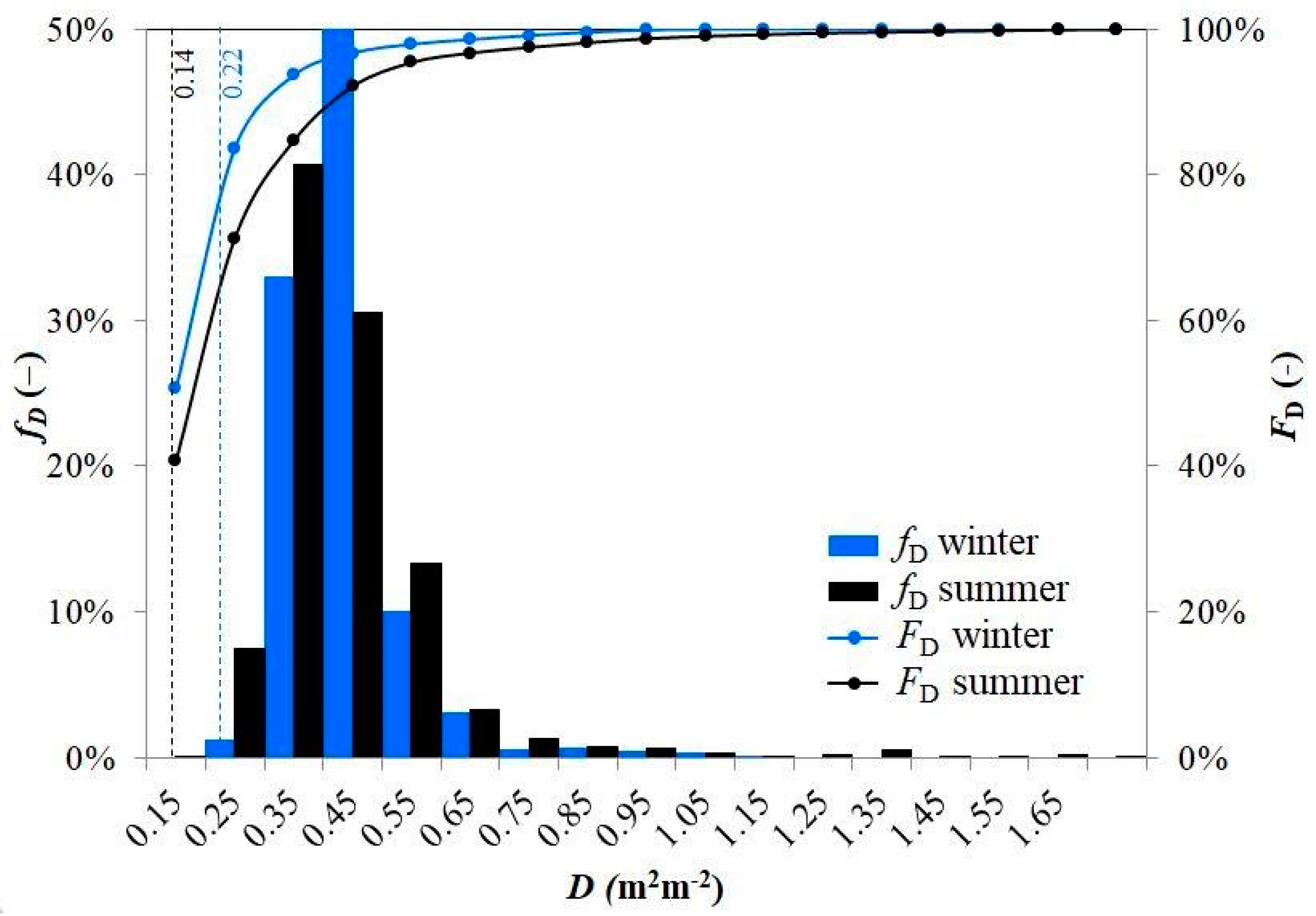
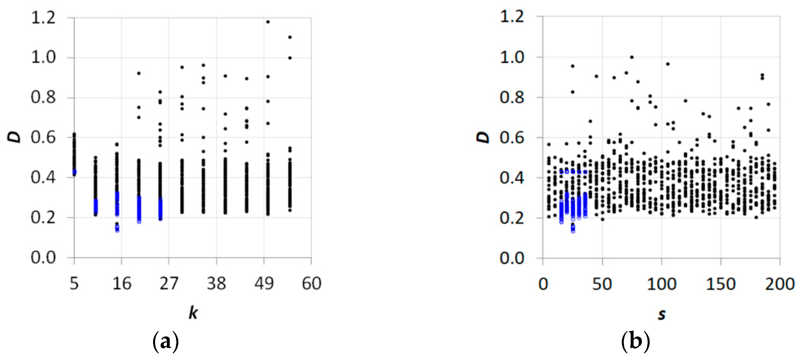
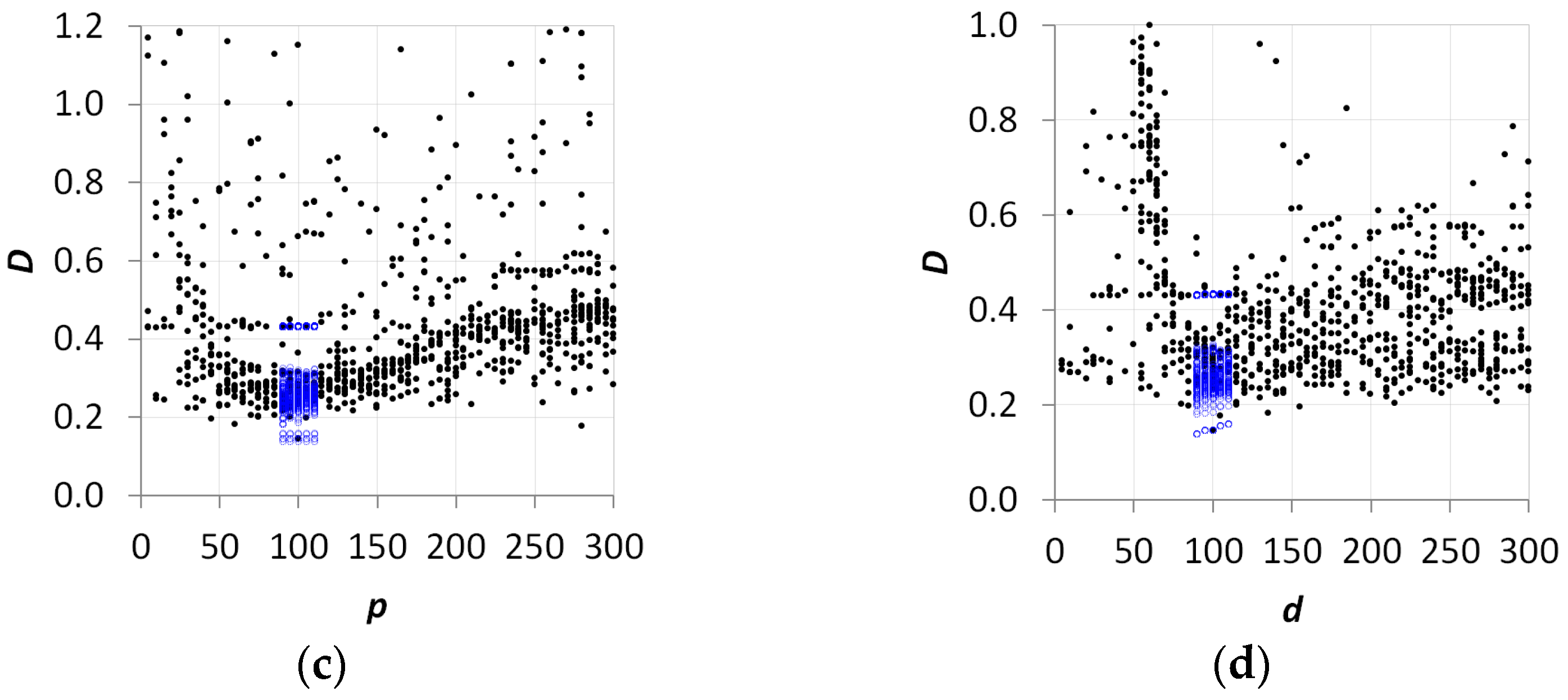
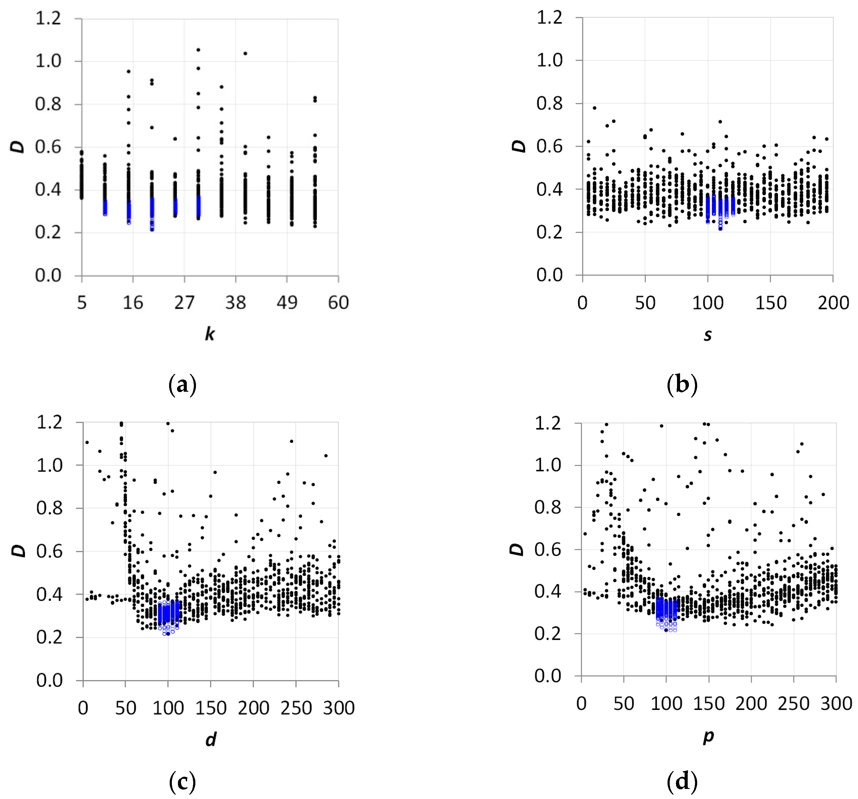
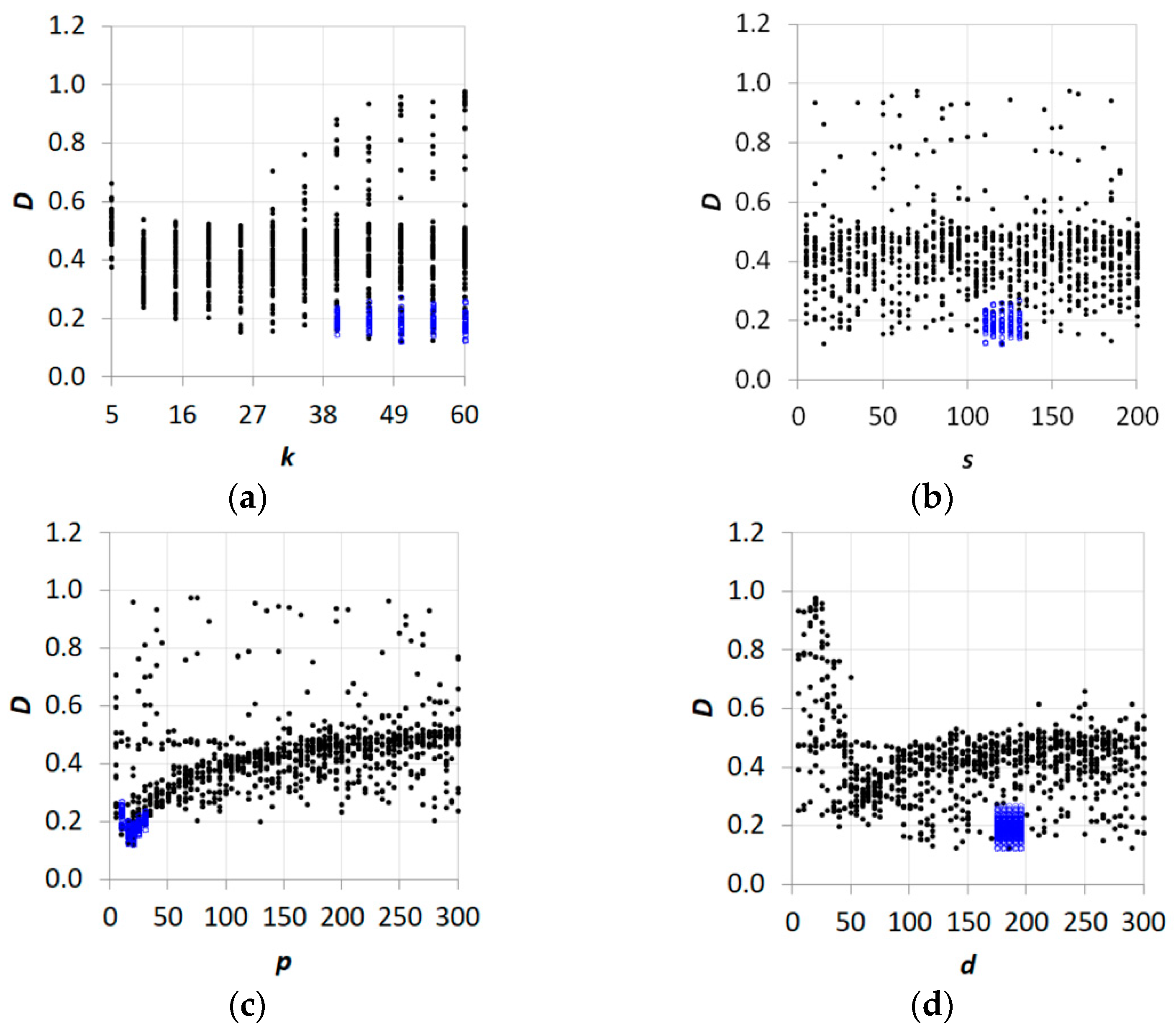
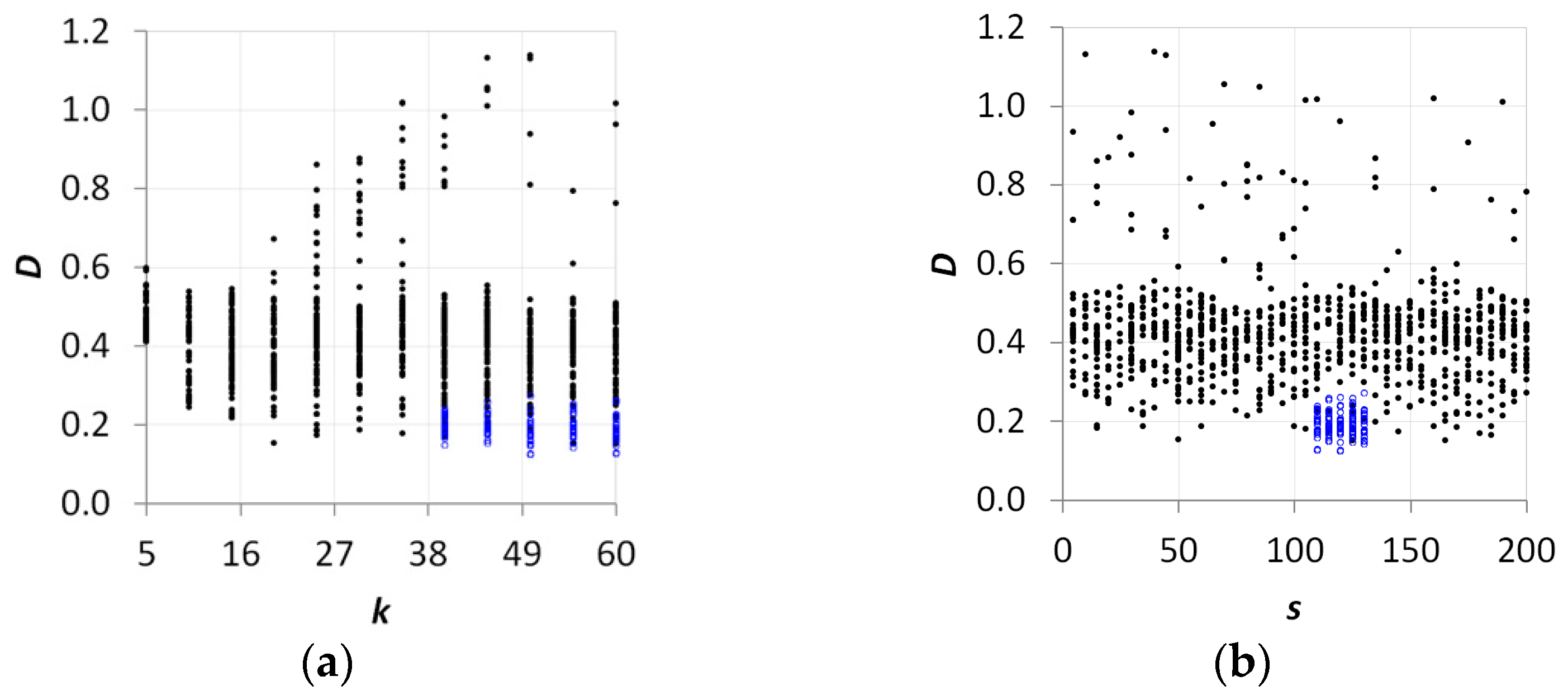
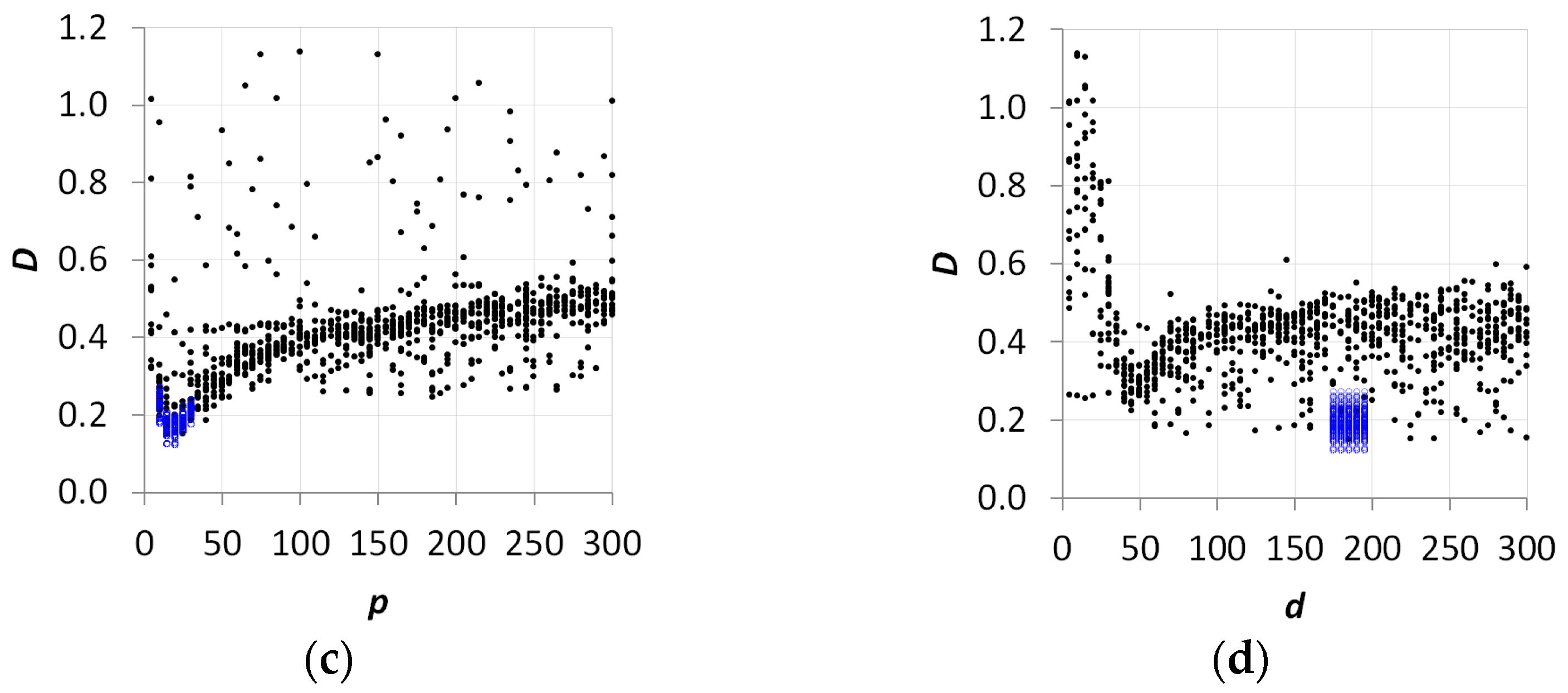
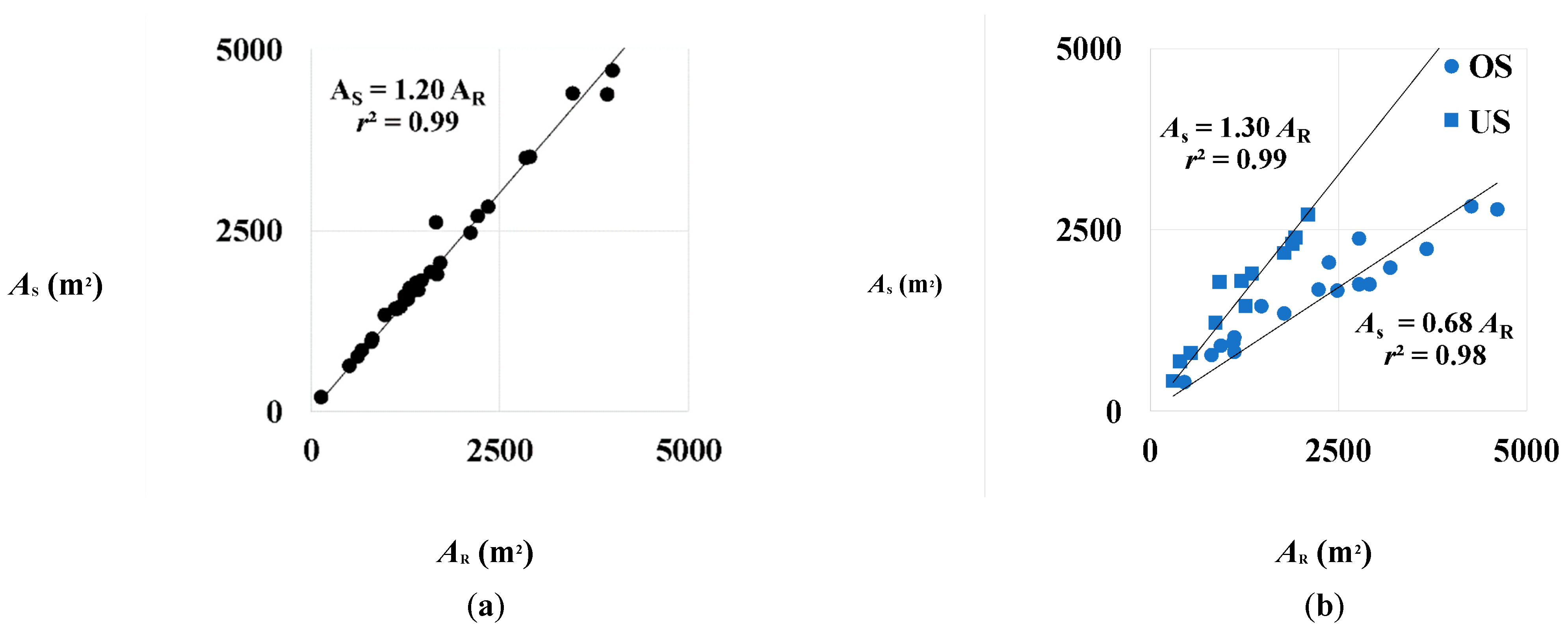
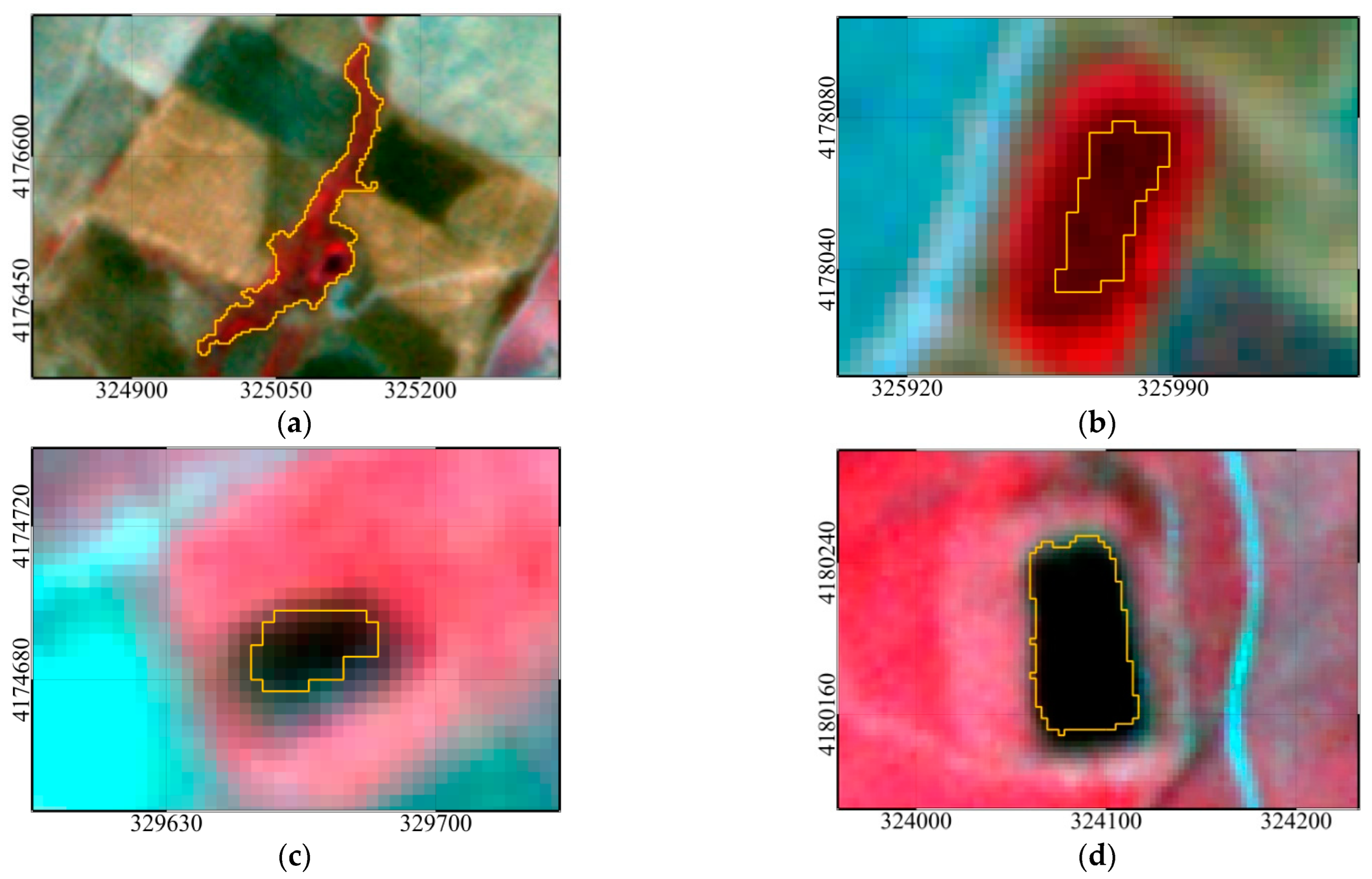
In this Section, the results obtained through segmentation, spectral separability and object-based classification are described.

3.1. Segmentation

The Python code, developed to optimize the segmentation of the hill lakes, was first trained on the areas, AR., of 30 lakes selected as the reference, then on their perimeters.
The best set of parameters was chosen through a domain reduction technique composed of two iterative phases: a first rough tuning and a final fine tuning.
The rough tuning on the areas of the reference lakes allowed for reducing the computational demand by narrowing the parameters’ domain of ~64–93% depending on the parameter.
The range of variability of the segmentation parameters was explored by selecting a discretization step equal to 10 during the rough tuning and then by selecting a discretization step equal to 5 during the fine tuning.
The fine tuning aimed to select the quadruple of parameters optimizing the matching of the areas or the perimeters of the selected reference lakes.
Generally, the mode of D (histogram peak in Figure 4) achieved in the pilot area in the arid period was lower (thus better) than in the temperate one.
The peak of the histogram representing the arid period, fD (black bars), is lower than that characterizing the temperate one (blue bars); thus, the FD curve for the pilot area representing the arid period is lower than the temperate one.
Segmentation parameters resulting from the rough and fine tuning were used for training the surface, and perimeters of the reference polygons for both pilot areas in the arid and temperate periods are reported (Figure 5, Figure 6, Figure 7 and Figure 8). Both D(k) and D(s) do not exhibit a clear range of variability (of k and s) to locate the minimum D. On the contrary, D(p) and D(d) decrease then increase, thus clearly showing a minimum.
The range explored in the second iteration (fine tuning, blue dots) resulted from the first iteration (rough tuning, black dots).
All the parameters’ combinations at step 5 were explored, resulting in 625 iterations.
Once refining the discretization step from 10 to 5, results indicate that the same value of D can be obtained with a different quadruple of parameters differing for just one parameter, thus highlighting that a discretization limit has been reached and any further refining of the discretization step would be worthless.
The best quadruple of parameters after the two iterations characterized the best matching between the areas of the segments with the areas of the reference lakes. The best quadruple of parameters allowed achieving DA ≅ 0.14 for the arid and DA ≅ 0.22 for the temperate (Table 1) periods; the ranges of the variability of the parameters explored through the two iterations are also shown between square brackets.
Of course, the best quadruple of parameters allowing the best matching with the area of the reference surface (minimum DA) in principle does not guarantee the best matching between the perimeters of the segments and the perimeters of the reference lakes (minimum DP) (Figure 8).
The best performances in terms of matching with the perimeters of the reference lakes were DP ≅ 0.12 for the pilot areas in the arid period and DP ≅ 0.15 for the temperate one (Table 2).
A comparison between areas AS and AR (Figure 9) shows that in the image representing the arid period (panel a), areas were overestimated (≅20% with an r2 ≅ 0.99); instead, in the one representing the temperate one (panel b), two different groups emerge. One of those overestimates the reference areas (≅30%, with a determination coefficient r2 ≅ 0.99), while the other underestimates the reference areas (≅32%, r2 ≅ 0.98).
The metric of the segmentation optimized to match the perimeters of the lakes was ≅0.12 for the arid period and ≅0.15 for the temperate one. Results highlight that the segmentation based on the reference areas performs more than that based on the reference perimeters; furthermore, the image acquired in the arid period is more suitable than that acquired in the temperate period also aiming to match the perimeters.
Given the broad interest in determining the surface of water bodies [23,83,84,85], segmented images were then classified based on the set of parameters determined by minimizing the metric for reference areas.

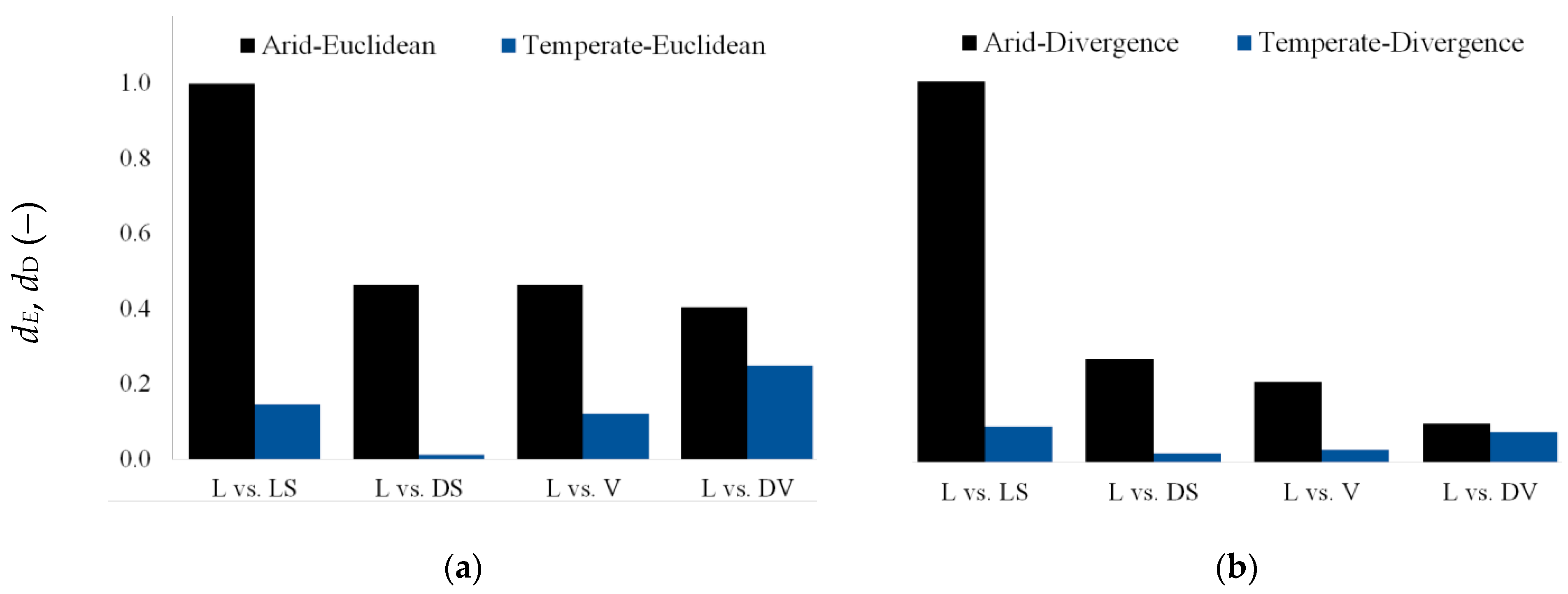
3.2. Spectral Separability

The Euclidean and divergence spectral separability metrics allowed for assessing the separability between hill lakes (L) versus dark soil (DS), light soil (LS), densely vegetated soil (DV) and vegetated soil (V), thus quantifying to what extent the L class can be confused with other classes (Figure 10).
Results show that, in the arid period, the densely vegetated soil class could be spectrally confused with the hill lakes’ class (dE = 0.40 and dD = 0.10); while in the temperate period, the dark soil class is the one that could be more easily misclassified with the hill lakes’ class (dE = 0.01 and dD = 0.02). The average dE and dD are reported in Table 3 to synthesize the effect of the period of acquisition on spectral separability.
Results indicate that images acquired in the arid period should be more suitable to distinguish the class hill lakes from other surfaces than those acquired in the temperate one. Indeed, the average separability using both the Euclidean and Divergence metrics in the arid period were ≅4-and 3-times higher than those obtained in the temperate one.

3.3. Classification

The NN and the RF algorithms were used to classify the pilot area and the whole catchment. The classification accuracies were evaluated both on the images representing the arid and temperate periods.
Here, a comparison of the lakes detected by classifying the pilot area in both arid and temperate periods (Figure 11) using the NN algorithm is shown.
The majority of the lakes (50) were classified by processing the image representing the arid period (UA = 1, PA ≅ 0.75), while six hill lakes were misclassified as dark soil and four as densely vegetated soil. Among these 10, only 1 misclassification was due to a segmentation error (densely vegetated soil). A lower number of lakes (37) were classified only by the image in the temperate period (UA ≅ 0.23, PA ≅ 0.58), while 23 dark soils were classified as hill lakes due to segmentation errors and five lakes were classified as dark soil due to classification errors. This could be due to the increasing similarity of the water and wet soil spectral signatures for increasing soil water content [86]. Using both the images representing the arid and temperate periods, 62 lakes out of 76 were identified in the pilot area.
It is worth highlighting that the segments selected from the two images are different. For quantifying the classification accuracy, 150 segments were selected (30 segments for each class) out of a total of ~20,000 segments, allowing one to reach a level of precision <0.1 (≈0.08).
By aggregating the classes into hill lakes versus other classes, the overall accuracy (OA ≅ 0.93 and ≅0.81 for the arid and temperate periods, respectively) confirms the outcomes of the spectral separability analysis. Indeed, the overall accuracy for the image representing the arid period is higher than that characterizing the temperate one (Table 4); accordingly, the dE for the arid period (black histograms in Figure 5) is higher than the one characterizing the temperate one (blue histogram). These accuracies decrease by 0.06 and 0.09 over the images representing the arid and temperate periods, respectively, after taking into account the agreement by chance. The Cohen coefficient K, indeed, was 0.68 over the image representing the arid period and 0.58 over the image representing the temperate one. Based on the Landis and Koch scale [82], the agreement beyond chance can be considered to be “substantial” (0.6 < K ≤ 0.8) for the arid period image and “moderate” (0.4 < K ≤ 0.6) for the temperate one.
After normalizing (Table 5) the error matrices, the overall accuracies increase to 0.87 and 0.72 for the images representing the arid and temperate periods. The agreement beyond chance increases as well to 0.83 and 0.65 to “almost perfect” and “substantial” agreement (arid and temperate periods, respectively).
Before normalization, the value of K was 8% lower than the OA in the arid period, and 13% lower than the OA in the temperate one. After normalization, the difference between K and OA was changed (it was reduced) due to the differences in the original marginal proportions; indeed, the value of K was 5% lower than the OA in the arid period and 10% lower than the OA in the temperate one.
The highest overall accuracy and agreement beyond chance are reached by classifying the image representing the arid period.
The lower spectral separability characterizing the hill lakes versus dark soil in the temperate period was confirmed by the accuracy assessment analyses; looking at Table 4, 23 of the 30 hill lakes used as reference were classified as dark soil instead of hill lakes.
To corroborate the indications of the NN classifier, the RF classifier was run over the same images. The PA values of the RF classification over the image representing the arid period resulted in a better performance compared to the NN classifier; additionally, the UA values of the RF classification confirmed an improved classification.
Over the image representing the temperate period, the PA values were better except for the LS and DS classes, while the UA values were worse compared to the NN classification except for the DS class.
Again, the RF classifier achieved better results over the image representing the arid period (the OA and K of the error matrix were equal to 0.90 and 0.88) and worse results over the image representing the temperate one (the OA and K were equal to 0.53 and 0.41).
Once accuracies are normalized, the PA values of the RF classification over the image representing the arid period confirmed the better performance of the RF compared to the NN classifier; furthermore, the UA values of the RF classification confirm the RF better performance as well.
Over the image representing the temperate period, the RF classifier resulted in higher PA values except for the L, DV and V classes, while the UA values were worse compared to the NN classification except for the L and DS classes. Overall, the OA and K of the normalized error matrix were equal to 0.91 and 0.89 over the arid period image and 0.71 and 0.64 over the temperate period image. However, not all the PA and UA values improved, although, as expected, the RF performed slightly more accurately, especially over the arid period image.
Then, as a result of the segmentation–classification procedure, some typical segmentation and classification errors are shown (Figure 12).
In the image representing the arid period, panel (a) shows that the lake is undersegmented; indeed, the segment includes the surrounding vegetation; panel (b) shows that although the lake is correctly segmented, it is misclassified as densely vegetated soil (DV).
In the image representing the temperate period, panel (c) shows that although the lake is correctly segmented, it is classified as dark soil (DS); finally, a lake that is accurately segmented and correctly classified is shown in panel (d).
By classifying the image of the arid period over the whole catchment, 531 of 797 lakes were identified. The OA and K over the whole study area were 0.69 and 0.62, respectively (Table 6), and these values increase to 0.72 and 0.65 after normalization. Based on the Landis and Koch scale [35], the agreement beyond chance can be considered as substantial (0.6 < K ≤ 0.8).
Of course, by aggregating the classes into hill lakes versus other classes, the overall accuracy increases (OA ≅ 0.88, no matrix normalization accounted for). Moreover, seasonal variations of the water level, mainly due to irrigation and rainfall, affect the extension of the reservoirs that are different in the two periods. However, the lake’s steep banks (45–60°) limit the variation of water surface area.

4. Conclusions

In conclusion, the proposed procedure was set up for analyzing the suitability of Earth observation periods for classifying features whose spectral separability change over time.
The procedure allowed one to describe the errors occurring both in the segmentation and classification phases of a GEOBIA algorithm. The spectral separability of the lakes from surrounding entities in the arid period is higher than in the temperate one: the average normalized Euclidean separability of water surfaces from soil and vegetation is ≈4-times higher than in the temperate period (≈3-times higher by considering the divergence metric).
Coherently, in the arid period, the metric of the segmentation optimized to match lakes’ areas was lower (≅0.14) than that achieved in the temperate one (≅0.22).
In accordance with the separability analysis, the classification using the Nearest Neighbor classifier returned a higher overall accuracy after normalization on the image representing the arid period (≅0.87 versus ≅0.72 in the temperate one). Moreover, the estimation of the extent of the lakes in the pilot area during the arid period was satisfying in terms of the determination coefficient (r2 ≅ 0.99), although it was characterized by an overestimation of 20%. It is worth highlighting that despite the seasonal variations of the water level, which depend on rainfall and irrigation seasons, the steepness of the banks limits the variation of the water surface.
An analysis of lakes’ classification errors highlights that: low producer accuracy in the pilot area during the arid and temperate periods (0.75 and 0.58, respectively) are mainly due to classification errors (9 of 10 in the pilot area during the arid period and 5 of 5 in the temperate one); user accuracy in the temperate period was unsatisfactory (0.23), implying that combining lakes classified through both images is not advisable.
However, further research is required to investigate the effect of the trophic level on the spectral separability of hill lakes from surrounding features since the water trophic state rules the irradiance water attenuation through the water column [87] and the water spectral reflectance [88] at the surface.
Additionally, results are representative of arid and temperate climates as classified by the Péguy climograph; however, other climate indexes [89] could be employed to select case studies representative of different climates worldwide.

Funding

This research received financial support from the Italian Ministry of Environment (Ministero dell’Ambiente e della Tutela del Territorio del Mare—Direzione Generale per la Salvaguardia del Territorio e delle Acque) through a scholarship under the project “LIMNADI—Integrazione muLti-scopo di piccoli Invasi collinari per la laMiNAzione Delle pIene”—CUP B76C18000890001.

Data Availability Statement

The data that support the findings of this study are openly available in the Knowledge Network for Biocomplexity repository at https://knb.ecoinformatics.org accessed on 20 November 2022, at https://doi.org/10.5063/F1X34VWC accessed on 20 November 2022.

Acknowledgments

The author expresses his gratitude to Eng. S. Buccafusco for implementing the hill lakes database and Eng, A. Paruta for implementing the Python code. Images were made available by Planet Labs Inc. (San Francisco, CA, USA) within the Planet’s Education and Research (E and R) Program.

Conflicts of Interest

No potential conflict of interest was reported by the author.

Abbreviations

AcronymMeaning
CIRCooler infrared
CRSCoordinates Reference Systems
DSDark soil
DVDensely vegetated soil
GEOBIAGeographic Object-Based Image Analysis
GISGeographic Information System
LHill lake
LSLight soil
MODISModerate Resolution Imaging Spectroradiometer
NIRNear Infrared
NNNearest Neighbor classifier
OBIAObject-Based Image Analysis
RFRandom Forest
RSGISLibRemote Sensing and GIS software library
SIASServizio Informativo Agrometereologico Siciliano, Sicilian agro-meteorological information service
VVegetated soil
VIIRSVisible Infrared Imaging Radiometer Suite
VISVisible

Appendix A

Table A1. List of Symbols.
SymbolMeaningUnit
A   ( R i S i ) Area of the intersection between the reference and segmented polygons(m2)
ARArea of the reference surfaces(m2)
ASArea of the segments(m2)
CLMisclassified entities(number)
Ci, CjCovariance matrices of the signatures i and j(—)
fDFrequency of occurrence of D(—)
FDCumulate of fD(—)
dDistance threshold for joining the segments(m)
dENormalized Euclidean distance(—)
dDNormalized Divergence(—)
DRoot mean square of the over and under segmentation quality metric(—)
DAD quality metric calibrated to match the areas of the reference polygons(—)
DPD quality metric calibrated to match the perimeters of the reference polygons(—)
eLevel of precision error(—)
kNumber of clusters(—)
KCohen’s kappa coefficient(—)
nNumber of reference segments(—)
NTotal number of segments(—)
NDVINormalized Difference Vegetation Index(—)
OAOverall accuracy(—)
OSOversegmentation(—)
pMinimum number of pixels within a segment(—)
PRPerimeter of the reference surfaces(m)
PSPerimeter of the segments(m)
PAProducer’s accuracy(—)
sSubsampling of the image for the data used within the segmentation(—)
SEMis-segmented entities(number)
UAUser’s accuracy(—)
USUndersegmentation(—)

References

  1. Baiocchi, V.; Brigante, R.; Dominici, D.; Milone, M.V.; Mormile, M.; Radicioni, F. Automatic Three-Dimensional Features Extraction: The Case Study of L’Aquila for Collapse Identification after April 06, 2009 Earthquake. Eur. J. Remote Sens. 2014, 47, 413–435. [Google Scholar] [CrossRef]
  2. Blaschke, T. Object Based Image Analysis for Remote Sensing. ISPRS J. Photogramm. Remote Sens. 2010, 65, 2–16. [Google Scholar] [CrossRef] [Green Version]
  3. Hossain, M.D.; Chen, D. Segmentation for Object-Based Image Analysis (OBIA): A Review of Algorithms and Challenges from Remote Sensing Perspective. ISPRS J. Photogramm. Remote Sens. 2019, 150, 115–134. [Google Scholar] [CrossRef]
  4. Blaschke, T.; Lang, S.; Lorup, E.; Strobl, J.; Zeil, P. Object-Oriented Image Processing in an Integrated GIS/Remote Sensing Environment and Perspectives for Environmental Applications. Environ. Inf. Plan. Politics Public 2000, 2, 555–570. [Google Scholar]
  5. Burnett, C.; Blaschke, T. A Multi-Scale Segmentation/Object Relationship Modelling Methodology for Landscape Analysis. Ecol. Model. 2003, 168, 233–249. [Google Scholar] [CrossRef]
  6. Ehlers, M.; Gähler, M.; Janowsky, R. Automated Analysis of Ultra High Resolution Remote Sensing Data for Biotope Type Mapping: New Possibilities and Challenges. ISPRS J. Photogramm. Remote Sens. 2003, 57, 315–326. [Google Scholar] [CrossRef]
  7. Lefèvre, S.; Sheeren, D.; Tasar, O. A Generic Framework for Combining Multiple Segmentations in Geographic Object-Based Image Analysis. ISPRS Int. J. Geo-Inf. 2019, 8, 70. [Google Scholar] [CrossRef] [Green Version]
  8. Johnson, B.; Xie, Z. Unsupervised Image Segmentation Evaluation and Refinement Using a Multi-Scale Approach. ISPRS J. Photogramm. Remote Sens. 2011, 66, 473–483. [Google Scholar] [CrossRef]
  9. Drăguţ, L.; Csillik, O.; Eisank, C.; Tiede, D. Automated Parameterisation for Multi-Scale Image Segmentation on Multiple Layers. ISPRS J. Photogramm. Remote Sens. 2014, 88, 119–127. [Google Scholar] [CrossRef] [Green Version]
  10. Zhao, H.; Chen, F.; Zhang, M. A Systematic Extraction Approach for Mapping Glacial Lakes in High Mountain Regions of Asia. IEEE J. Sel. Top. Appl. Earth Obs. Remote Sens. 2018, 11, 2788–2799. [Google Scholar] [CrossRef]
  11. Gao, B. NDWI—A Normalized Difference Water Index for Remote Sensing of Vegetation Liquid Water from Space. Remote Sens. Environ. 1996, 58, 257–266. [Google Scholar] [CrossRef]
  12. Cimtay, Y.; Özbay, B.; Yilmaz, G.; Bozdemir, E. A New Vegetation Index in Short-Wave Infrared Region of Electromagnetic Spectrum. IEEE Access 2021, 9, 148535–148545. [Google Scholar] [CrossRef]
  13. Li, S.; Sun, D.; Yu, Y.; Csiszar, I.; Stefanidis, A.; Goldberg, M.D. A New Short-Wave Infrared (SWIR) Method for Quantitative Water Fraction Derivation and Evaluation With EOS/MODIS and Landsat/TM Data. IEEE Trans. Geosci. Remote Sens. 2013, 51, 1852–1862. [Google Scholar] [CrossRef]
  14. Zhang, M.; Zhao, H.; Chen, F.; Zeng, J. Evaluation of Effective Spectral Features for Glacial Lake Mapping by Using Landsat-8 OLI Imagery. J. Mt. Sci. 2020, 17, 2707–2723. [Google Scholar] [CrossRef]
  15. Talineau, J.-C.; Selmi, S.; Alaya, K. Lacs collinaires en Tunisie semi-aride. Sci. Et Changements Planétaires/Sécheresse 1994, 5, 251–256. [Google Scholar]
  16. Boufaroua, M.; Slimani, M.; Oweis, T.; Alberge, J. Hill Lakes: Innovative Approach for Sustainable Rural Management in the Semi-Arid Areas in Tunisia. Glob. NEST J. 2013, 15, 366–373. [Google Scholar] [CrossRef]
  17. Deep Learning for Extracting Water Body from Landsat Imagery. Semantic Scholar. Available online: https://www.semanticscholar.org/paper/DEEP-LEARNING-FOR-EXTRACTING-WATER-BODY-FROM-Yang-Tian/220b6d870bc3616ac3cf9d9801000c4f16bdcd7c (accessed on 14 December 2021).
  18. Amitrano, D.; Martino, G.D.; Iodice, A.; Riccio, D.; Ruello, G. Small Reservoirs Extraction in Semiarid Regions Using Multitemporal Synthetic Aperture Radar Images. IEEE J. Sel. Top. Appl. Earth Obs. Remote Sens. 2017, 10, 3482–3492. [Google Scholar] [CrossRef]
  19. Kaplan, G.; Avdan, U. Object-Based Water Body Extraction Model Using Sentinel-2 Satellite Imagery. Eur. J. Remote Sens. 2017, 50, 137–143. [Google Scholar] [CrossRef] [Green Version]
  20. Liebe, J.R.; van de Giesen, N.; Andreini, M.S.; Steenhuis, T.S.; Walter, M.T. Suitability and Limitations of ENVISAT ASAR for Monitoring Small Reservoirs in a Semiarid Area. IEEE Trans. Geosci. Remote Sens. 2009, 47, 1536–1547. [Google Scholar] [CrossRef]
  21. Small, C.; Okujeni, A.; van der Linden, S.; Waske, B. 6.07—Remote Sensing of Urban Environments. In Comprehensive Remote Sensing; Liang, S., Ed.; Elsevier: Oxford, UK, 2018; pp. 96–127. ISBN 978-0-12-803221-3. [Google Scholar]
  22. Liang, S.; Wang, J. (Eds.) Chapter 1—A Systematic View of Remote Sensing. In Advanced Remote Sensing, 2nd ed.; Academic Press: Cambridge, MA, USA, 2020; pp. 1–57. ISBN 978-0-12-815826-5. [Google Scholar]
  23. Liuzzo, L.; Puleo, V.; Nizza, S.; Freni, G. Parameterization of a Bayesian Normalized Difference Water Index for Surface Water Detection. Geosciences 2020, 10, 260. [Google Scholar] [CrossRef]
  24. Sarzana, T.; Maltese, A.; Capolupo, A.; Tarantino, E. Post-Processing of Pixel and Object-Based Land Cover Classifications of Very High Spatial Resolution Images. In Lecture Notes in Computer Science; Springer: Berlin/Heidelberg, Germany, 2020; Volume 12252, pp. 797–812. [Google Scholar] [CrossRef]
  25. Casadei, S.; Di Francesco, S.; Giannone, F.; Pierleoni, A. Small Reservoirs for a Sustainable Water Resources Management. Adv. Geosci. 2019, 49, 165–174. [Google Scholar] [CrossRef]
  26. Péguy, C.-P. Une tentative de délimitation et de schématisation des climats intertropicaux. Géocarrefour 1961, 36, 1–6. [Google Scholar] [CrossRef]
  27. Regione Siciliana Assessorato Agricoltura e Foreste, Gruppo IV—Servizi Allo Sviluppo, Unità di Agrometeorologia Climatologia della Sicilia. Available online: http://www.sias.regione.sicilia.it/ (accessed on 24 December 2022).
  28. Regione Siciliana Assessorato Risorse Agricole e Alimentari Dipartimento Interventi Strutturali SIAS—Servizio Informativo Agrometeorologico Siciliano. Available online: http://www.sias.regione.sicilia.it/ (accessed on 24 December 2022).
  29. Didan, K. MOD13Q1 MODIS/Terra Vegetation Indices 16-Day L3 Global 250 m SIN Grid V006. 2015. Available online: https://lpdaac.usgs.gov/products/mod13q1v006/ (accessed on 24 December 2022).
  30. van Leeuwen, W.J.D.; Huete, A.R.; Laing, T.W. MODIS Vegetation Index Compositing Approach: A Prototype with AVHRR Data. Remote Sens. Environ. 1999, 69, 264–280. [Google Scholar] [CrossRef]
  31. ORNL DAAC. MODIS and VIIRS Land Products Global Subsetting and Visualization Tool; ORNL DAAC: Oak Ridge, TN, USA, 2018. [CrossRef]
  32. Capodici, F.; Cammalleri, C.; Francipane, A.; Ciraolo, G.; La Loggia, G.; Maltese, A. Soil Water Content Diachronic Mapping: An FFT Frequency Analysis of a Temperature–Vegetation Index. Geosciences 2020, 10, 23. [Google Scholar] [CrossRef] [Green Version]
  33. Dey, V.; Zhang, Y.; Zhong, M. A Review on Image Segmentation Techniques with Remote Sensing Perspective. Environ. Sci. 2010, 38, 31–42. [Google Scholar]
  34. Jackson, J.A. Automated Image Segmentation for Synthetic Aperture Radar Feature Extraction. In Proceedings of the IEEE 2010 National Aerospace & Electronics Conference, Dayton, OH, USA, 14–16 July 2010; pp. 45–49. [Google Scholar]
  35. Wang, S.-H.; Sun, J.; Phillips, P.; Zhao, G.; Zhang, Y.-D. Polarimetric Synthetic Aperture Radar Image Segmentation by Convolutional Neural Network Using Graphical Processing Units. J. Real-Time Image Process. 2018, 15, 631–642. [Google Scholar] [CrossRef]
  36. Gautam, S.; Singhai, J. Cosine-Similarity Watershed Algorithm for Water-Body Segmentation Applying Deep Neural Network Classifier. Environ. Earth Sci. 2022, 81, 251. [Google Scholar] [CrossRef]
  37. Babu, A.A.; Rajam, V.M.A. Water-Body Segmentation from Satellite Images Using Kapur’s Entropy-Based Thresholding Method. Comput. Intell. 2020, 36, 1242–1260. [Google Scholar] [CrossRef]
  38. Duan, L.; Hu, X. Multiscale Refinement Network for Water-Body Segmentation in High-Resolution Satellite Imagery. IEEE Geosci. Remote Sens. Lett. 2020, 17, 686–690. [Google Scholar] [CrossRef]
  39. Li, Z.; Wang, R.; Zhang, W.; Hu, F.; Meng, L. Multiscale Features Supported DeepLabV3+ Optimization Scheme for Accurate Water Semantic Segmentation. IEEE Access 2019, 7, 155787–155804. [Google Scholar] [CrossRef]
  40. Miao, Z.; Fu, K.; Sun, H.; Sun, X.; Yan, M. Automatic Water-Body Segmentation From High-Resolution Satellite Images via Deep Networks. IEEE Geosci. Remote Sens. Lett. 2018, 15, 602–606. [Google Scholar] [CrossRef]
  41. Weng, L.; Xu, Y.; Xia, M.; Zhang, Y.; Liu, J.; Xu, Y. Water Areas Segmentation from Remote Sensing Images Using a Separable Residual SegNet Network. ISPRS Int. J. Geo-Inf. 2020, 9, 256. [Google Scholar] [CrossRef]
  42. Yuan, K.; Zhuang, X.; Schaefer, G.; Feng, J.; Guan, L.; Fang, H. Deep-Learning-Based Multispectral Satellite Image Segmentation for Water Body Detection. IEEE J. Sel. Top. Appl. Earth Obs. Remote Sens. 2021, 14, 7422–7434. [Google Scholar] [CrossRef]
  43. Zhang, Z.; Lu, M.; Ji, S.; Yu, H.; Nie, C. Rich CNN Features for Water-Body Segmentation from Very High Resolution Aerial and Satellite Imagery. Remote Sens. 2021, 13, 1912. [Google Scholar] [CrossRef]
  44. Felzenszwalb, P.F.; Huttenlocher, D.P. Efficient Graph-Based Image Segmentation. Int. J. Comput. Vis. 2004, 59, 167–181. [Google Scholar] [CrossRef]
  45. Shepherd, J.D.; Bunting, P.; Dymond, J.R. Operational Large-Scale Segmentation of Imagery Based on Iterative Elimination. Remote Sens. 2019, 11, 658. [Google Scholar] [CrossRef] [Green Version]
  46. Bunting, P.; Clewley, D.; Lucas, R.M.; Gillingham, S. Remote Sensing and GIS Software Library (RSGISLib). Comput. Geosci. 2014, 62, 216–226. [Google Scholar] [CrossRef]
  47. Chen, Y.; Chen, Q.; Jing, C. Multi-Resolution Segmentation Parameters Optimization and Evaluation for VHR Remote Sensing Image Based on MeanNSQI and Discrepancy Measure. J. Spat. Sci. 2021, 66, 253–278. [Google Scholar] [CrossRef]
  48. Karakış, S.; Marangoz, A.; Buyuksalih, G. Analysis of Segmentation Parameters in Ecognition Software Using High Resolution Quickbird Ms Imagery. In Proceedings of the ISPRS Workshop on Topographic Mapping from Space, Ankara, Turkey, 14–16 February 2006. [Google Scholar]
  49. Mean Shift: A Robust Approach toward Feature Space Analysis|IEEE Journals & Magazine|IEEE Xplore. Available online: https://ieeexplore.ieee.org/document/1000236 (accessed on 16 July 2022).
  50. Michel, J.; Feuvrier, T.; Inglada, J. Reference Algorithm Implementations in OTB: Textbook Cases. In Proceedings of the 2009 IEEE International Geoscience and Remote Sensing Symposium, Cape Town, South Africa, 12–17 July 2009; Volume 4, pp. IV-741–IV-744. [Google Scholar]
  51. Liu, Y.; Bian, L.; Meng, Y.; Wang, H.; Zhang, S.; Yang, Y.; Shao, X.; Wang, B. Discrepancy Measures for Selecting Optimal Combination of Parameter Values in Object-Based Image Analysis. ISPRS J. Photogramm. Remote Sens. 2012, 68, 144–156. [Google Scholar] [CrossRef]
  52. El-naggar, A.M. Determination of Optimum Segmentation Parameter Values for Extracting Building from Remote Sensing Images. Alex. Eng. J. 2018, 57, 3089–3097. [Google Scholar] [CrossRef]
  53. Weidner, U. Contribution to the Assessment of Segmentation Quality for Remote Sensing Applications. Int. Arch. Photogramm. Remote Sens. 2008, 37, 479–484. [Google Scholar]
  54. Eisank, C.; Smith, M.; Hillier, J. Assessment of Multiresolution Segmentation for Delimiting Drumlins in Digital Elevation Models. Geomorphology 2014, 214, 452–464. [Google Scholar] [CrossRef]
  55. Ramezan, C.A.; Warner, T.A.; Maxwell, A.E. Evaluation of Sampling and Cross-Validation Tuning Strategies for Regional-Scale Machine Learning Classification. Remote Sens. 2019, 11, 185. [Google Scholar] [CrossRef] [Green Version]
  56. Puranik, Y.; Sahinidis, N.V. Domain Reduction Techniques for Global NLP and MINLP Optimization. Constraints 2017, 22, 338–376. [Google Scholar] [CrossRef] [Green Version]
  57. Swain, P.H.; Davis, S.M. (Eds.) Remote Sensing; The Quantitative Approach; McGraw-Hill College: London, UK; New York, NY, USA, 1979; ISBN 978-0-07-062576-1. [Google Scholar]
  58. Swain, P.H.; Davis, S.M. Remote Sensing: The Quantitative Approach. IEEE Trans. Pattern Anal. Mach. Intell. 1981, PAMI-3, 713–714. [Google Scholar] [CrossRef]
  59. Shivakumar, B.R.; Rajashekararadhya, S.V. Spectral Similarity for Evaluating Classification Performance of Traditional Classifiers. In Proceedings of the 2017 International Conference on Wireless Communications, Signal Processing and Networking, Chennai, India, 22–24 March 2017; pp. 1999–2004. [Google Scholar]
  60. Optimum Band Selection for Supervised Classification of Multispectral Data. Semantic Scholar. Available online: https://www.semanticscholar.org/paper/Optimum-Band-Selection-for-Supervised-of-Data/9693651d1240e3034a8049fbc0cd1c5cbaf65428 (accessed on 13 December 2021).
  61. Renard, X.; Laugel, T.; Detyniecki, M. Understanding Prediction Discrepancies in Machine Learning Classifiers. arXiv 2021, arXiv:2104.05467. [Google Scholar]
  62. Pedregosa, F.; Varoquaux, G.; Gramfort, A.; Michel, V.; Thirion, B.; Grisel, O.; Blondel, M.; Müller, A.; Nothman, J.; Louppe, G.; et al. Scikit-Learn: Machine Learning in Python. arXiv 2018, arXiv:1201.0490. [Google Scholar]
  63. Mountrakis, G.; Im, J.; Ogole, C. Support Vector Machines in Remote Sensing: A Review. ISPRS J. Photogramm. Remote Sens. 2011, 66, 247–259. [Google Scholar] [CrossRef]
  64. Sharma, R.; Ghosh, A.; Joshi, P.K. Decision Tree Approach for Classification of Remotely Sensed Satellite Data Using Open Source Support. J. Earth Syst. Sci. 2013, 122, 1237–1247. [Google Scholar] [CrossRef] [Green Version]
  65. Miller, D.M.; Kaminsky, E.J.; Rana, S. Neural Network Classification of Remote-Sensing Data. Comput. Geosci. 1995, 21, 377–386. [Google Scholar] [CrossRef]
  66. Seidl, T. Nearest Neighbor Classification. In Encyclopedia of Database Systems; Liu, L., Özsu, M.T., Eds.; Springer: Boston, MA, USA, 2009; pp. 1885–1890. ISBN 978-0-387-39940-9. [Google Scholar]
  67. Yamane, T. Statistics: An Introductory Analysis, 2nd ed.; Harper and Row: New York, NY, USA, 1967. [Google Scholar]
  68. Nkomeje, F. Comparative Performance of Multi-Source Reference Data to Assess the Accuracy of Classified Remotely Sensed Imagery: Example of Landsat 8 OLI Across Kigali City-Rwanda 2015. Int. J. Eng. Work. 2017, 4, 10–20. [Google Scholar]
  69. Hoekstra, M.; Jiang, M.; Clausi, D.A.; Duguay, C. Lake Ice-Water Classification of RADARSAT-2 Images by Integrating IRGS Segmentation with Pixel-Based Random Forest Labeling. Remote Sens. 2020, 12, 1425. [Google Scholar] [CrossRef]
  70. Geurts, P.; Ernst, D.; Wehenkel, L. Extremely Randomized Trees. Mach. Learn. 2006, 63, 3–42. [Google Scholar] [CrossRef] [Green Version]
  71. Story, M.; Congalton, R.G. Accuracy Assessment: A User’s Perspective. Photogramm. Eng. Remote Sens. 1986, 52, 397–399. [Google Scholar]
  72. Cohen, J. A Coefficient of Agreement for Nominal Scales. Educ. Psychol. Meas. 1960, 20, 37–46. [Google Scholar] [CrossRef]
  73. Rwanga, S.S.; Ndambuki, J.M. Accuracy Assessment of Land Use/Land Cover Classification Using Remote Sensing and GIS. IJG 2017, 8, 611–622. [Google Scholar] [CrossRef]
  74. Analysis of Classification Results of Remotely Sensed Data and Evaluation of Classification Algorithms. Semantic Scholar. Available online: https://www.semanticscholar.org/paper/Analysis-of-classification-results-of-remotely-data-Zhuang-Engel/58e57a879542a0a7711eebc6d7311555731da9b8 (accessed on 27 December 2021).
  75. Smits, P.C.; Dellepiane, S.G.; Schowengerdt, R.A. Quality Assessment of Image Classification Algorithms for Land-Cover Mapping: A Review and a Proposal for a Cost-Based Approach. Int. J. Remote Sens. 1999, 20, 1461–1486. [Google Scholar] [CrossRef]
  76. Congalton, R.G.; Oderwald, R.G.; Mead, R.A. Assessing Landsat Classification Accuracy Using Discrete Multivariate Analysis Statistical Techniques. Photogramm. Eng. Remote Sens. 1983, 49, 1671–1678. [Google Scholar]
  77. Agresti, A.; Ghosh, A.; Bini, M. Raking Kappa: Describing Potential Impact of Marginal Distributions on Measures of Agreement. Biom. J. 1995, 37, 811–820. [Google Scholar] [CrossRef]
  78. Stehman, S.V. A Critical Evaluation of the Normalized Error Matrix in Map Accuracy Assessment. Photogramm. Eng. Remote Sens. 2004, 70, 743–751. [Google Scholar] [CrossRef]
  79. Byrt, T.; Bishop, J.; Carlin, J.B. Bias, Prevalence and Kappa. J. Clin. Epidemiol. 1993, 46, 423–429. [Google Scholar] [CrossRef] [PubMed]
  80. Fleiss, J.L.; Levin, B.; Paik, M.C.; Fleiss, J. Statistical Methods for Rates & Proportions, 3rd ed.; Wiley-Interscience: Hoboken, NJ, USA, 2003; ISBN 978-0-471-52629-2. [Google Scholar]
  81. Monserud, R.A.; Leemans, R. Comparing Global Vegetation Maps with the Kappa Statistic. Ecol. Model. 1992, 62, 275–293. [Google Scholar] [CrossRef]
  82. Landis, J.R.; Koch, G.G. The Measurement of Observer Agreement for Categorical Data. Biometrics 1977, 33, 159–174. [Google Scholar] [CrossRef] [Green Version]
  83. Avisse, N.; Tilmant, A.; Müller, M.F.; Zhang, H. Monitoring Small Reservoirs’ Storage with Satellite Remote Sensing in Inaccessible Areas. Hydrol. Earth Syst. Sci. 2017, 21, 6445–6459. [Google Scholar] [CrossRef] [Green Version]
  84. Pipitone, C.; Maltese, A.; Dardanelli, G.; Brutto, M.L.; Loggia, G.L. Monitoring Water Surface and Level of a Reservoir Using Different Remote Sensing Approaches and Comparison with Dam Displacements Evaluated via GNSS. Remote Sens. 2018, 10, 71. [Google Scholar] [CrossRef] [Green Version]
  85. Maltese, A.; Pipitone, C.; Dardanelli, G.; Capodici, F.; Muller, J.-P. Toward a Comprehensive Dam Monitoring: On-Site and Remote-Retrieved Forcing Factors and Resulting Displacements (GNSS and PS–InSAR). Remote Sens. 2021, 13, 1543. [Google Scholar] [CrossRef]
  86. Divya, Y.; Gopinathan, P. Soil Water Content Measurement Using Hyper-Spectral Remote Sensing Techniques—A Case Study from North-Western Part of Tamil Nadu, India. Remote Sens. Appl. Soc. Environ. 2019, 14, 1–7. [Google Scholar] [CrossRef]
  87. Ciraolo, G.; Cox, E.; La Loggia, G.; Maltese, A. The Classification of Submerged Vegetation Using Hyperspectral MIVIS Data. Ann. Geophys. 2006, 49, 287–294. [Google Scholar] [CrossRef]
  88. Liu, H.; He, B.; Zhou, Y.; Kutser, T.; Toming, K.; Feng, Q.; Yang, X.; Fu, C.; Yang, F.; Li, W.; et al. Trophic State Assessment of Optically Diverse Lakes Using Sentinel-3-Derived Trophic Level Index. Int. J. Appl. Earth Obs. Geoinf. 2022, 114, 103026. [Google Scholar] [CrossRef]
  89. Zepner, L.; Karrasch, P.; Wiemann, F.; Bernard, L. ClimateCharts.Net—An Interactive Climate Analysis Web Platform. Int. J. Digit. Earth 2021, 14, 338–356. [Google Scholar] [CrossRef]
Figure 1. Location map: (a) Italy (light green) in Europe (light grey); (b) the river basin (dashed polygon) in Sicily (light green, south Italy) over-imposed the pilot area (blue rectangle). Coordinates Reference Systems (CRS) were chosen according to the Decree 10 November 2011 entitled “Adoption of the National Geodetic Reference System” issued by the Presidency of the Council of Ministers of Italy (Official Gazette General Series n.48 of 27 February 2012—Ordinary Suppl. n. 37).
Remotesensing 15 00262 g001
Figure 2. Pilot area. CIR composition of the selected images for the arid (a) and temperate (b) periods.
Remotesensing 15 00262 g002
Figure 3. Flowchart of the procedure to test the proposed method.
Remotesensing 15 00262 g003
Figure 4. On the primary y-axis, the frequency of occurrence of D, fD, as the output of the segmentation calibration code (pilot areas representing arid and temperate periods in black and blue histograms, respectively). On the secondary y-axis, the cumulate of fD, FD, (dotted lines).
Remotesensing 15 00262 g004
Figure 5. Segmentation parameters optimized on reference areas in the arid period (black dots represent values resulting from the rough; blue dots represent values resulting from the fine-tuning): (a) D versus k; (b) D versus p; (c) D versus s; (d) D versus d, dispersions.
Remotesensing 15 00262 g005aRemotesensing 15 00262 g005b
Figure 6. Segmentation parameters optimized on reference areas in the temperate period: (a) D versus k; (b) D versus p; (c) D versus s; (d) D versus d, dispersions.
Remotesensing 15 00262 g006
Figure 7. Segmentation parameters optimized on perimeters for the arid period: (a) D versus k; (b) D versus p; (c) D versus s; (d) D versus d, dispersions.
Remotesensing 15 00262 g007
Figure 8. Segmentation parameters optimized on perimeters for the temperate period: (a) D versus k; (b) D versus p; (c) D versus s; (d) D versus d, dispersions.
Remotesensing 15 00262 g008aRemotesensing 15 00262 g008b
Figure 9. Performance in terms of surface estimation: surface as the output of the GEOBIA procedure, AS, of the 30 reference lakes vs. surfaces of digitized lakes, AR, for the images representing the arid (a) and the temperate (b) periods.
Remotesensing 15 00262 g009
Figure 10. Histogram of the separability distance for the pilot areas representing the arid (black) and temperate (blue) periods: (a) normalized Euclidean distance, dE; (b) normalized divergence, dD.
Remotesensing 15 00262 g010
Figure 11. Spatial distribution of the hill lakes in the pilot area resulting from the segmentation-classification process. Cyan points represent lakes identified both from the images representing the arid and temperate periods; black points identify lakes classified only in the arid period; blue points identify lakes classified only in the temperate one.
Remotesensing 15 00262 g011
Figure 12. Segmentation or classification issues (yellow line bounded polygons) overimposed to the CIR composition of the images representing the arid and temperate periods (upper and lower panels, respectively): (a) erroneous segmentation; (b,c) misclassification; (d) correct segmentation and classification.
Remotesensing 15 00262 g012
Table 1. Segmentation parameters, images acquired in arid and temperate periods.
kSPdDA
1st phase range: both[5, 60][5, 200][5, 300][5, 300]
2nd phase range: arid[5, 25][15, 35][90, 110][90, 110]
temperate[10, 30][100, 120][90, 110][90, 110]
best parameters: arid1525105900.14
temperate20110105950.22
Table 2. Segmentation parameters and images acquired in arid and temperate periods.
kSpdDP
1st phase range: both[5, 60][5, 200][5, 300][5, 300]
2nd phase range: arid[40, 60][110, 130][10, 30][175, 195]
temperate[45, 65][115, 135][5, 25][175, 195]
best parameters: arid50120201850.12
temperate55125151850.15
Table 3. Average normalized spectral separability using all the spectral bands for both the Euclidean and the divergence metrics in the arid and temperate periods.
EuclideanDivergence
Pilot area, arid period0.490.39
Pilot area, temperate period0.120.14
Table 4. Error matrix of the NN classification. When the achieved accuracy is higher than that achieved by the RF classifier, its value is underlined.
Classified
Arid PeriodTemperate Period
LLSDSDVVPALLSDSDVVPA
ReferenceL3006
(CL)
4
(3CL + 1SE)
00.75705
(CL)
000.58
LS0204000.830271110.90
DS0315000.8323 (SE)322620.39
DV0002370.770021810.86
V0753230.610005260.84
UA10.670.500.770.77 0.230.900.730.600.87
OA0.740.67
K0.680.58
Table 5. Normalized error matrix of the NN classification. When the achieved normalized accuracy is higher than that achieved by the RF classifier, its value is underlined.
Classified
Arid PeriodTemperate Period
LLSDSDVVPALLSDSDVVPA
ReferenceL1000010.5800.42000.58
LS00.830.17000.8300.930.030.020.020.93
DS00.170.83000.830.420.070.410.070.030.41
DV0000.830.170.83000.140.790.060.88
V0000.160.830.830000.120.880.88
UA10.830.830.830.83 0.580.930.410.790.88
OA0.870.72
K0.830.65
Table 6. Accuracy assessment of the image of the arid period over the whole basin.
Classified
Not Normalized Error MatrixNormalized Error Matrix
LLSDSDVVPALLSDSDVVPA
ReferenceL2104230.700.7100.150.050.080.71
LS0242020.8600.830.1000.070.83
DS7321750.490.170.060.560.110.100.56
DV2021800.820.1200.140.7400.75
V0313200.7400.110.050.090.750.75
UA0.700.800.700.600.67 0.710.830.560.740.75
OA0.690.72
K0.620.65
Disclaimer/Publisher’s Note: The statements, opinions and data contained in all publications are solely those of the individual author(s) and contributor(s) and not of MDPI and/or the editor(s). MDPI and/or the editor(s) disclaim responsibility for any injury to people or property resulting from any ideas, methods, instructions or products referred to in the content.

