Generating Paired Seismic Training Data with Cycle-Consistent Adversarial Networks

Abstract

Deep-learning-based seismic data interpretation has received extensive attention and focus in recent years. Research has shown that training data play a key role in the process of intelligent seismic interpretation. At present, the main methods used to obtain training data are synthesizing seismic data and manually labeling the real data. However, synthetic data have certain feature differences from real data, and the manual labeling of data is time-consuming and subjective. These factors limit the application of deep learning algorithms in seismic data interpretation. To obtain realistic seismic training data, we propose label-to-data networks based on cycle-consistent adversarial networks in this work. These networks take random labels and unlabeled real seismic data as input and generate synthetic seismic data that match the random labels and have similar features to the real seismic data. Quantitative analysis of the generated data demonstrate the effectiveness of the proposed methods. Meanwhile, test results on different data indicate that the generated data are reliable and can be applied for seismic fault detection.

1. Introduction

Detection of subsurface structures from seismic data plays a significant role in seismic data interpretation. Among the various subsurface structures, faults are important since they can behave as a seal or a conduit for oil and gas transportation, and fault fracture zones are also favorable spaces for hydrocarbon accumulation in carbonate rock areas. In conventional fault interpretation, interpreters detect faults according to the reflection discontinuity or steep dipping of seismic data. Subsequently, fault detection has been implemented through seismic attribute technologies or image processing technologies, such as coherence attribute [1,2], texture attribute [3], curvature attribute [4], edge detection [5], and guided filtering [6], among others.

With the advent of convolutional neural networks (CNNs) [7] and the development of deep learning algorithms, various CNN-based methods have been introduced to assist in geophysical problems, such as seismic inversion [8], horizon tracking [9], seismic data interpolation and reconstruction [10], first-arrival picking [11], seismic data denoising [12,13,14], and so on. In particular, they play an important role in the detection and interpretation of seismic faults.

Most seismic fault detection methods based on deep learning fall into two categories, either based on image classification or image segmentation. Wu et al. [15] and Zheng et al. [16] used synthetic fault samples and multi-classification CNNs to implement fault detection. They classified faults according to the dip or azimuth and visualized the classification results. Xiong et al. [17] and Di et al. [18] used manually labeled samples to achieve fault detection. The difference is that Xiong et al. adopted two-classification CNNs, while Di et al. chose support vector machine (SVM)/multi-layer perceptron (MLP) classification algorithms. Wu et al. [19] and Liu et al. [20] synthesized three-dimensional seismic fault data and used end-to-end U-Net image segmentation networks to implement three-dimensional fault detection. The segmentation networks are capable of pixel-level classification, and the detection results of the segmentation networks are generally better than classification networks. For better detection results, Wu et al. [21] improved the three-dimensional seismic structure models to make the synthetic data more realistic. Then, they built image segmentation networks to achieve seismic fault and horizon interpretation.

Considering the above research, it is clear that the common strategy to obtain fault training data is through synthesizing and labeling manually. However, synthetic data have certain characteristic differences from real data, including the complexity of structures, the frequency of the data, the type or intensity of the noise, and so on. Meanwhile, manually labeling a large number of faults is time-consuming and lacks objectivity. To solve these problems, Cunha et al. [22] and Yan et al. [23] used synthetic fault training samples to pre-train CNNs, and then transferred [24] the network by using a small number of real data to improve the detection results. Di et al. [25] developed a framework for integrating seismic interpretation CNNs with common knowledge and rules as constraints to obtain the desired results. Durall et al. [26] introduced generative models to improve the authenticity of synthetic data. Specifically, they made the synthetic fault samples more similar to the real samples through data transformation. Ferreira et al. [27] proposed a method for synthesizing seismic images from simple sketches using deep generative networks. This approach has the potential to be applied to the synthesis of fault data but it is supervised learning approach, as the method requires paired training data and labels. Li et al. [28] and Feng et al. [29] used variational autoencoders (VAE) to augment the seismic data and alleviated the problem of lacking labeled seismic data for supervised learning.

In this study, we aim to utilize unlabeled seismic data and random fault labels to generate realistic seismic faults images and we propose label-to-data networks based on Cycle-consistent adversarial networks (CycleGAN) [30], providing a theoretical background for the transformation of random labels into seismic fault data. The networks can generate paired seismic training data by learning the unpaired labels and real data. The generated data are similar to real data, and the locations of faults match the input labels. This method can generate realistic training data while avoiding the use of complex functions to build models or manual fault labeling. Then, fault training data are generated with different features and validated by different methods. Next, we trained U-Nets [31] with the generated data and detected faults in real data. The experimental results on seismic data demonstrated that the fault training data are reliable and realistic, and label-to-data networks can effectively solve the problems related to data shortages.

2. Methods

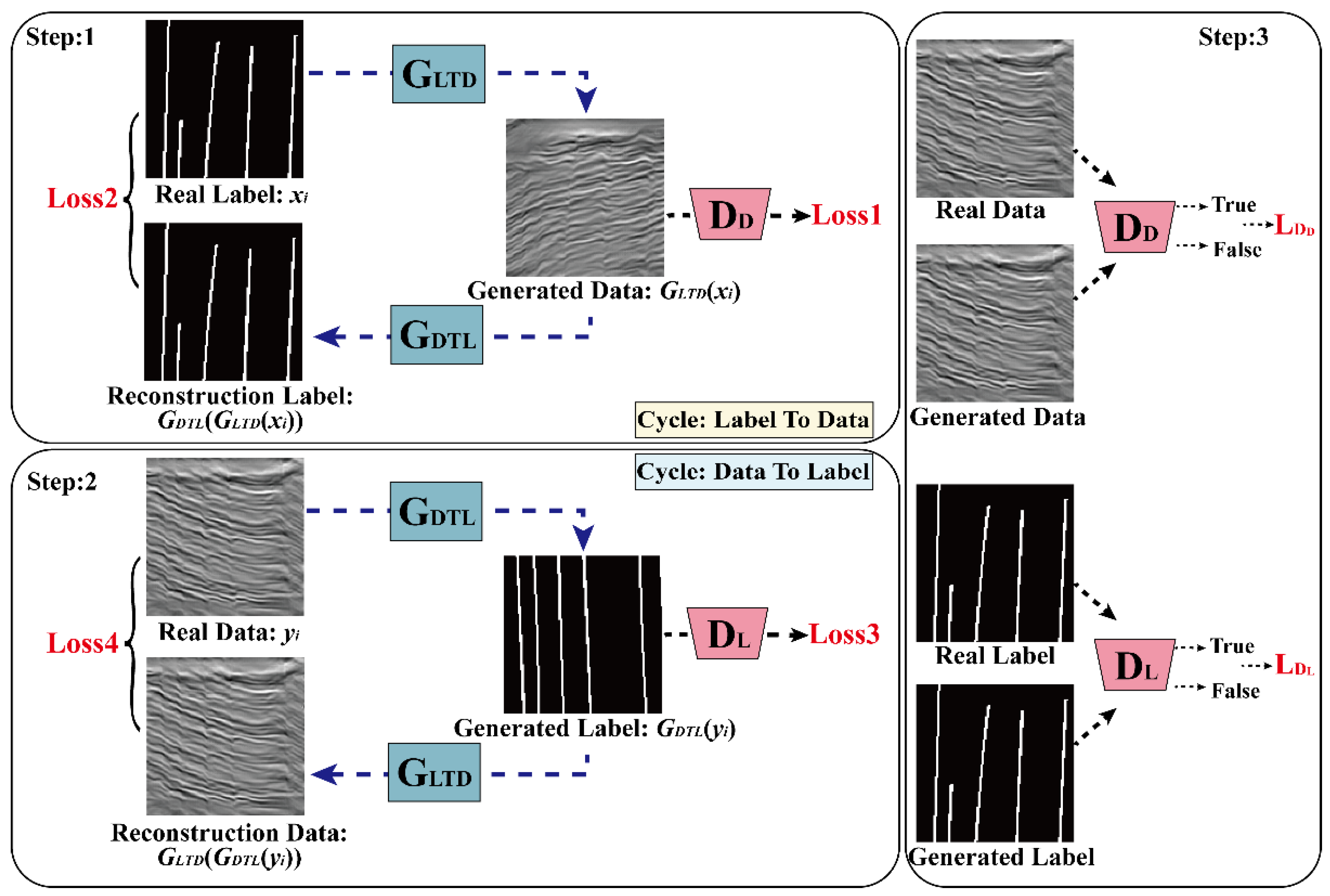
2.1. Cycle-Consistent Adversarial Networks

Generative adversarial nets (GANs) [32] are methods that generate similar synthetic data by learning the features of input data. They are mainly composed of two parts: one is the generator G, and the other is the discriminator D. G captures the data features and generates synthetic data. Then, D estimates whether the data is real or synthetic. The generator G is trained to generate synthetic data which are highly similar to real data, such that D cannot discriminate between the two. The optimization purpose for D involves enhancing its discrimination ability and reducing errors. However, the generation process is random, and it cannot be ensured that a generated image and input data are paired. Dong et al. [13] used GAN to generate random noise data, and the generated noise and the real noise have a similar distribution. Therefore, researchers have proposed image-to-image adversarial networks [33]. Image-to-image methods can ensure that images and labels are paired after the transformation; however, such approaches belong to the category of supervised learning, which requires paired data as input. Such a requirement is difficult to satisfy when using seismic data. To achieve the image-to-image translation task without paired data, CycleGAN has been proposed. It is an unsupervised data transformation method which can achieve image generation and retain original features in the absence of paired samples. Thus, we adopt the scheme of seismic training samples generation based on CycleGAN.

Figure 1 illustrates the inputs and outputs of our proposed label-to-data networks, the first column shows the input labels, while the second column shows the input samples. The labels were randomly generated. For each label, we create a 128 × 128 array with all values of 0, and then add some random lines to the array with values of 1 as fault labels, and the length, dip, and number of faults are random within a certain range. Although the generated labels are random, they should conform to the geological rules. The samples were randomly cropped from the sections of Kerry3D data (provided on the SEG Wiki). The number of labels and seismic samples is 1000, and they do not need to be paired. The fourth and fifth columns show another set of labels and unpaired real data. This real data acquired from China, denoted as Data1, and 1000 samples are cropped from the sections of Data1. The output (columns 3 and 6) of the well-trained CycleGAN was anticipated to be able to match the input labels (columns 1 and 4), while maintaining similar features to the input seismic images (columns 2 and 5). Thus, we can obtain massive seismic training images and corresponding fault labels.

2.2. Label-to-Data Networks and Training Process

Taking the Kerry fault samples as an example, the label-to-data network structure is shown in Figure 2. The main structure includes two generators and two discriminators, and their structural details are shown in Figure 3. In this paper, we define the input labels as X, with x_i ∈ X representing the ith label in X, and the input seismic images as Y, with y_i ∈ Y representing the ith seismic image in Y. The generators and the discriminators are trained separately in each epoch. The training process for each epoch consists of three steps.

Step 1: input the real label to the generator G_LTD to obtain the generated data. The discriminator D_D discriminates the authenticity of generated data and calculates the adversarial loss (Loss1; Equation (2)) using the MSE loss function. Then, the generated data are input into the generator G_DTL to obtain the reconstruction label, and the cycle consistency loss (Loss2; Equation (3)) between the real label and reconstruction label is calculated using the MAE loss function.

Step 2: calculate Loss3 (Equation (4)) and Loss4 (Equation (5)) in the same process as in Step 1. Sum Loss1–Loss4 to obtain L_G (Equation (1)), and optimize both G_LTD and G_DTL using L_G.

$$\begin{array}{l}{L}_G\left(G_{LTD},G_{DTL},D_D,D_L,X,Y\right)=\\ [Loss1\left(G_{LTD},D_D,x_i\right)+Loss2\left(G_{LTD},G_{DTL},x_i\right)\\ +Loss3\left(G_{DTL},D_L,y_i\right)+Loss4\left(G_{LTD},G_{DTL},y_i\right)]\end{array}$$

(1)

$$Loss1\left(G_{LTD},D_D,x_i\right)=\frac{1}{N}{\displaystyle \sum }_{i=1}^N{\left[D_D\left(G_{LTD}\left(x_i\right)\right)-1\right]}^2$$

(2)

$$Loss2\left(G_{LTD},G_{DTL},x_i\right)=\frac{1}{N}{\displaystyle \sum }_{i=1}^N\left|G_{DTL}\left(G_{LTD}\left(x_i\right)\right)-x_i\right|$$

(3)

$$Loss3\left(G_{DTL},D_L,y_i\right)=\frac{1}{N}{\displaystyle \sum }_{i=1}^N{\left[D_L\left(G_{DTL}\left(y_i\right)\right)-1\right]}^2$$

(4)

$$Loss4\left(G_{DTL},G_{LTD},y_i\right)=\frac{1}{N}{\displaystyle \sum }_{i=1}^N\left|G_{LTD}\left(G_{DTL}\left(y_i\right)\right)-y_i\right|$$

(5)

Step 3: input real and generated data to D_D, and real and generated labels to D_L, respectively. D_D and D_L then determine the authenticity of the input and calculate $L_{D_D}$ (Equation (6)) and $L_{D_L}$ (Equation (7)) losses, respectively. D_D and D_L are optimized using $L_{D_D}$ and $L_{D_L},$ respectively. At this point, an epoch is completed, and all networks are optimized.

$$L_{D_D}=\frac{1}{N}{\displaystyle \sum }_{i=1}^N\left[{\left(D_D\left(y_i\right)-1\right)}^2+{\left(D_D\left(G_{LTD}\left(x_i\right)\right)\right)}^2\right]$$

(6)

$$L_{D_L}=\frac{1}{N}{\displaystyle \sum }_{i=1}^N\left[{\left(D_L\left(x_i\right)-1\right)}^2+{\left(D_L\left(G_{DTL}\left(y_i\right)\right)\right)}^2\right]$$

(7)

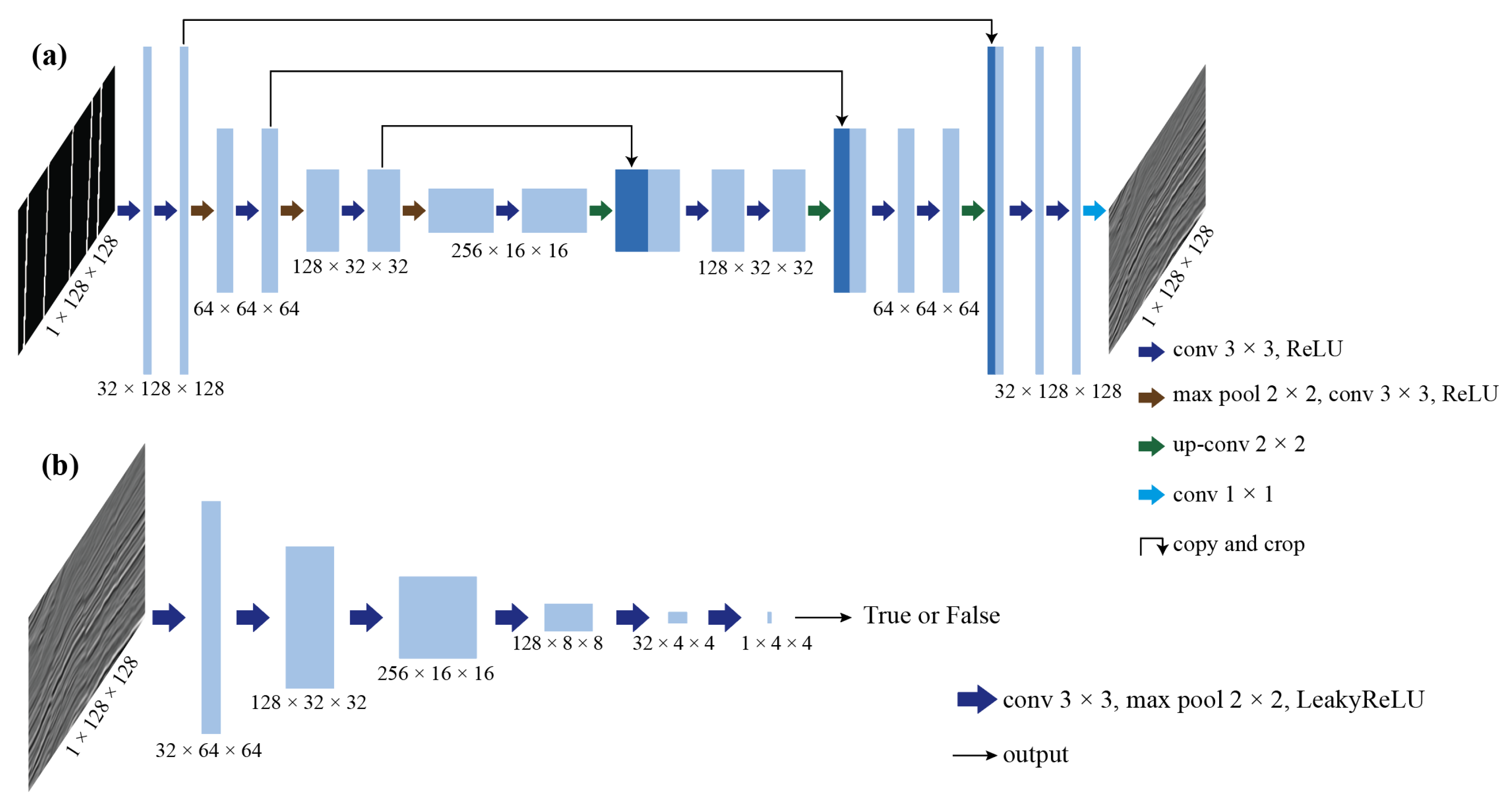
2.3. Networks Parameters and Training details

Both G_LTD and G_DTL have a U-Net structure (Figure 3a). The input is a single channel label image of size 128 × 128 pixels and the output is the generated seismic image (of the same size). The maximum number of channels in the networks is 256, and the data are down- and up-sampled three times each. Both D_D and D_L have a six-layer CNN structure (Figure 3b). The input is a real or generated image of size 128 × 128 pixels, and the output is the discrimination result. Assuming the image is true, this output should be 1; otherwise, it is 0. We prepared 1000 labels and seismic samples for training, and set the training epoch to 200, batch size to 10, a learning rate of G to 5 × 10⁻⁵, and a learning rate of D to 1 × 10⁻⁴. The optimization algorithm was Adam [34]. In addition, the weights of Loss1–Loss4 can be adjusted according to the real situation. For example, when G_LTD cannot transform labels into seismic data well, the weight of Loss1 should be increased. We built the networks using PyTorch, then trained the models on an RTX 3090. The training process takes 34 minutes. By the end of the training, the labels could be transformed into seismic data by G_LTD, and the transformation process took 12 seconds for 1000 samples.

3. Results

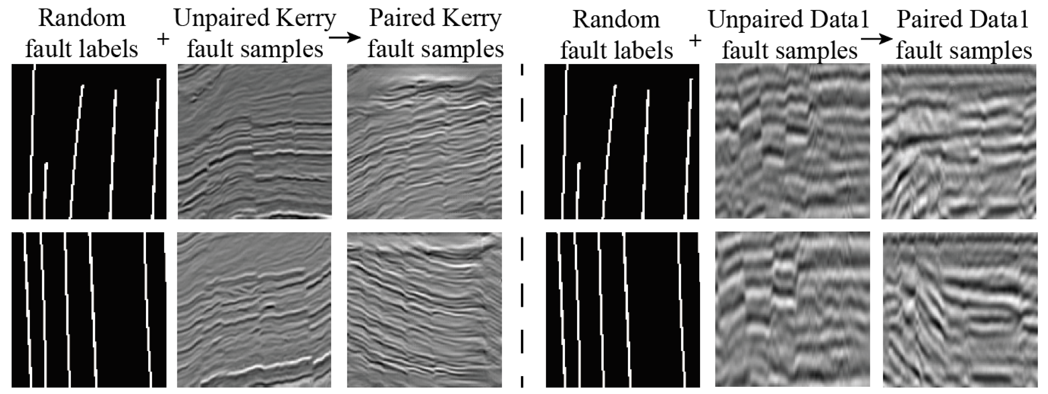
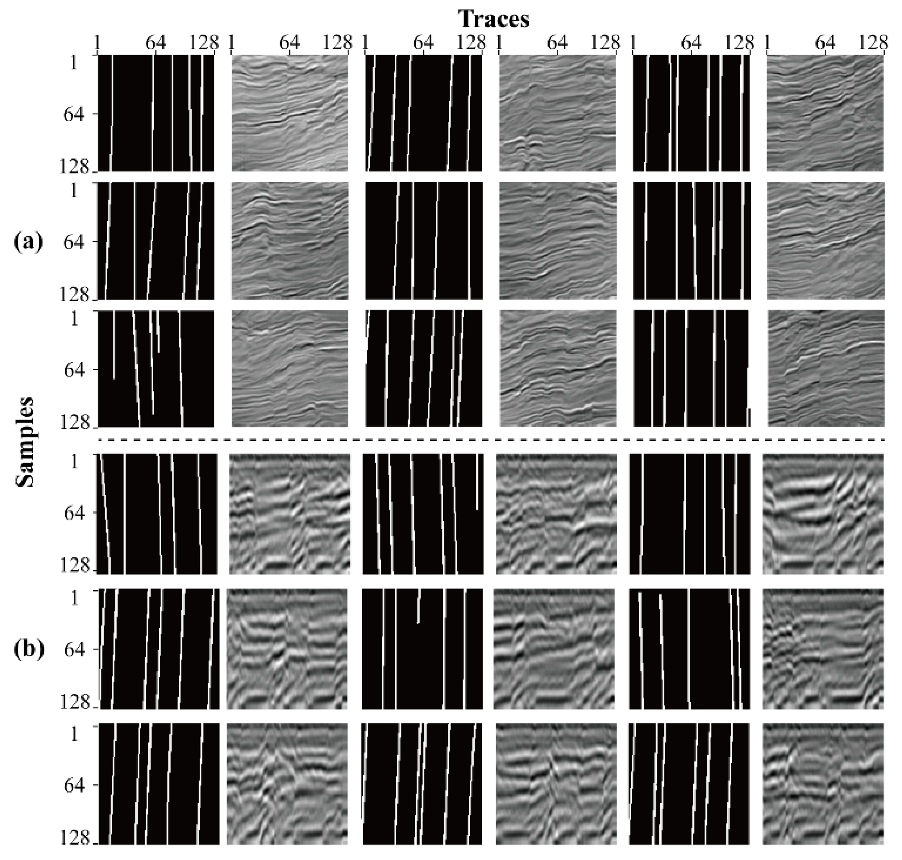
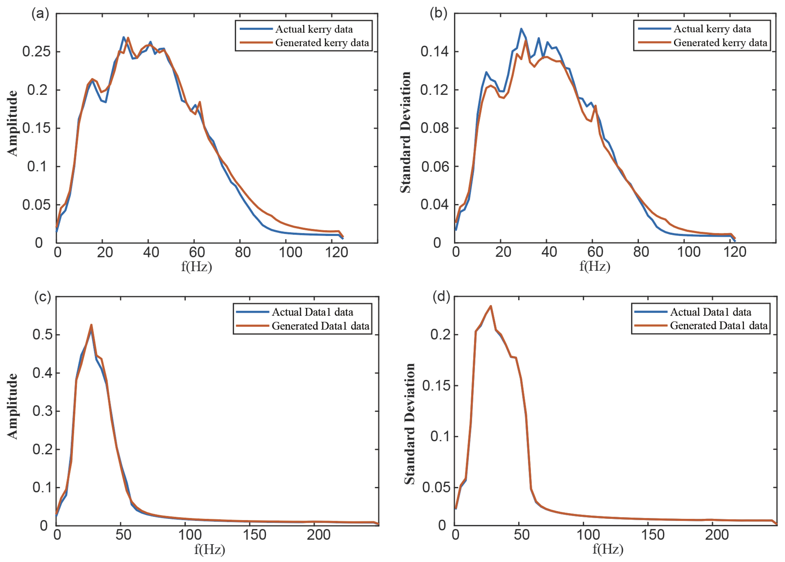
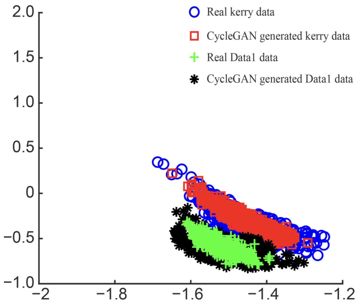
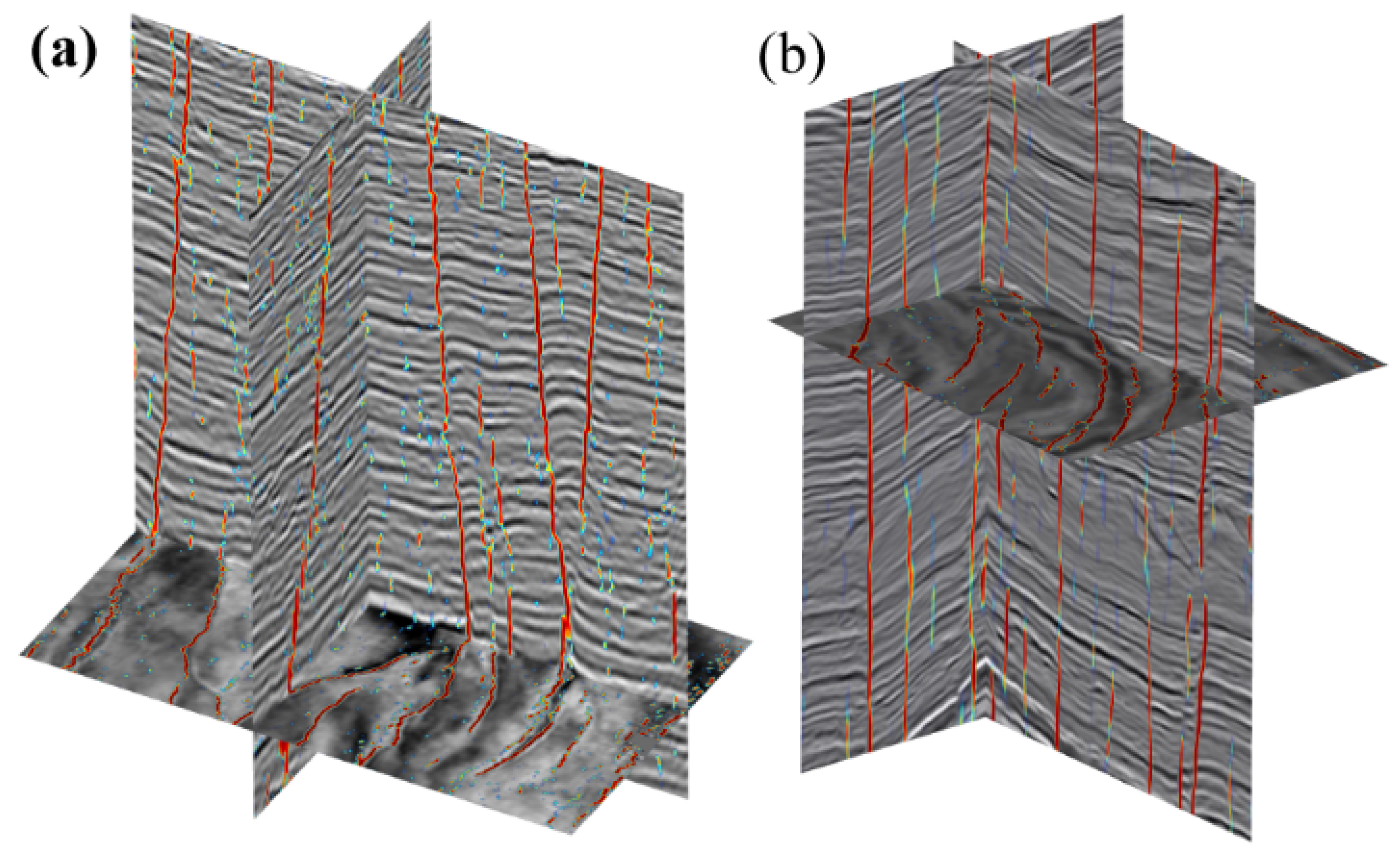
3.1. Application in Kerry3D and Data1 Samples Generation

We chose two real data sets to test the proposed networks: one was a subset (Inline 537–785, Crossline 190–537, Time 128–1756 ms) of Kerry3D, and the other was Data1. A total of 1000 random fault labels were prepared and 1000 samples were randomly cropped to a size of 128 × 128 from the sections of Kerry3D and Data1, respectively. After training, the labels were transformed into paired Kerry and Data1 fault images (as shown in Figure 4a,b) using the saved G_LTD models.

To quantitatively analyze the similarity between the generated and real data, the average frequency spectra and the standard deviation of the different frequencies were calculated on different data sets. The results are shown in Figure 5, which indicates that the generated and real images had similar frequency spectra. Then, we computed six of the Haralick textural features [35] (i.e., Angular Second Moment, Contrast, Correlation, Inverse Difference Moment, Sum Entropy, and Difference Variance) on the different data sets and the texture dissimilarity was obtained in two dimensions (as shown in Figure 6) using the multi-dimensional scaling (MDS) method [36]. The vertical and horizontal axes are dimensionless, and they indicate the extent of textural dissimilarity. Figure 6 shows that the generated Data1 and Kerry data had similar textural features to the real Data1 and Kerry data, respectively. The textural features of the generated Data1 and Kerry data differed, indicating that the generated data were target-oriented.

To validate whether the generated Kerry and Data1 data can be applied for fault detection, we trained two U-Nets with the generated Kerry and Data1 data. The two U-Nets with a structure similar to that shown in Figure 3a, but the parameters of networks, training samples, and loss functions (binary cross entropy) are completely different, and these U-Nets are used for fault detection testing. For convenience, we denote the network trained with generated Kerry3D samples as Net1 and the network trained with Data1 samples as Net2. Then, we applied Net1 and Net2 to different Kerry and Data1 sections, respectively. We set the window size to 128 and the window overlap to 64. Using a sliding window is a common method in the field of seismic structure detection, as the overlap enables faults at the image edges to be detected correctly. Figure 7 displays two Kerry test sections with the associated detection results. The locations indicated by the yellow arrows show that the prediction was accurate and continuous. This network could recognize most faults continuously, even in the low SNR portion from 0.8–1.0 seconds. The locations indicated by the black arrows indicate where the prediction was discontinuous or omission was detected. We consider the reason for omission detection is that the training data were not sufficient and generated images did not have similar fault features. Figure 8 displays two Data1 test sections with detection results, and the arrows in Figure 8 have the same meaning as above. Figure 9 shows a 3D view of detection results for Data1 and Kerry.

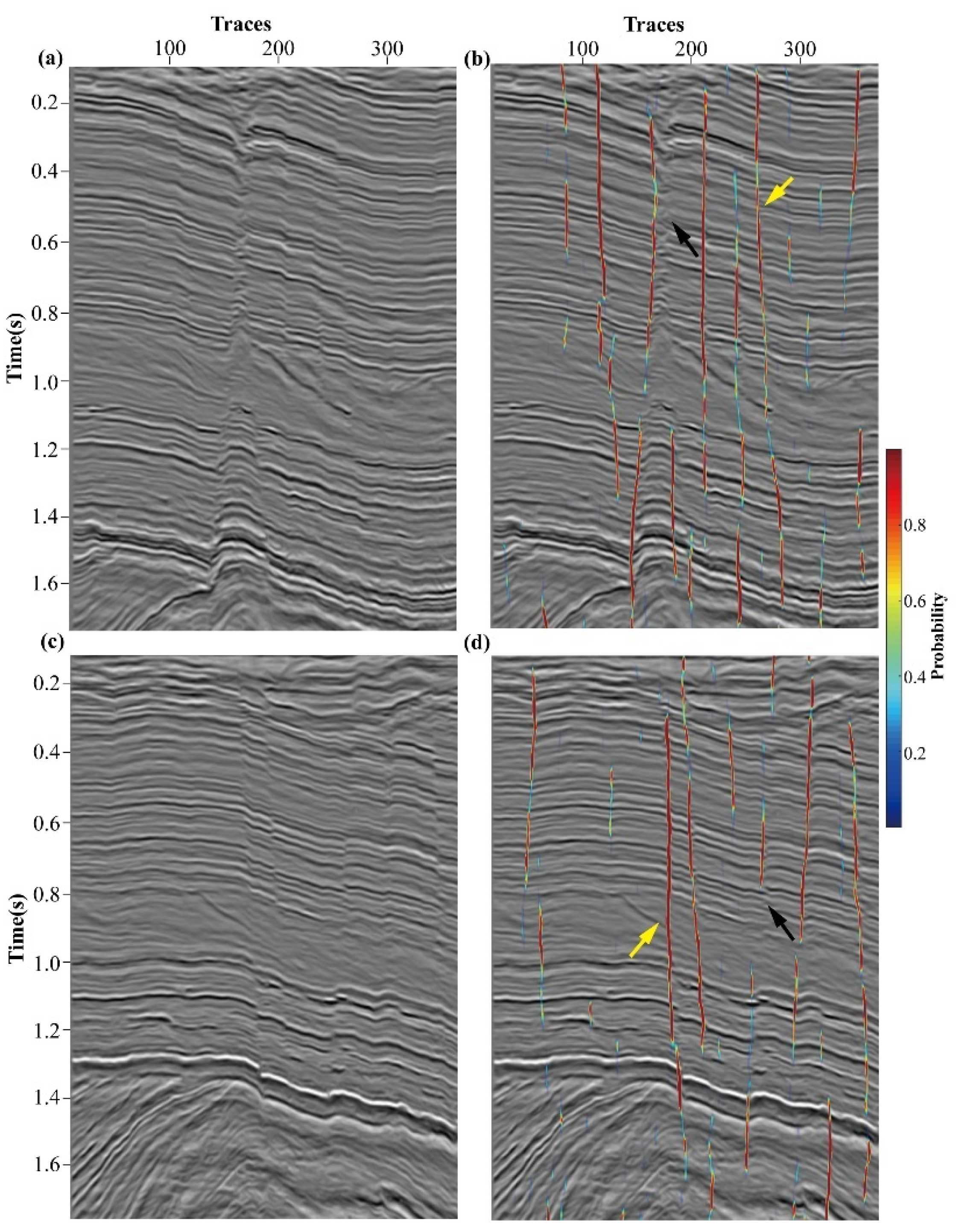
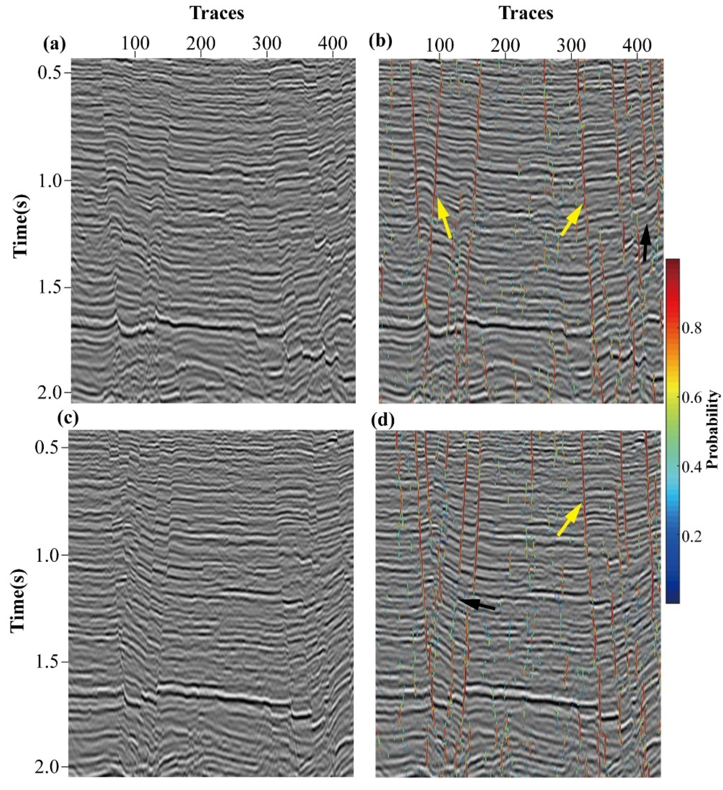
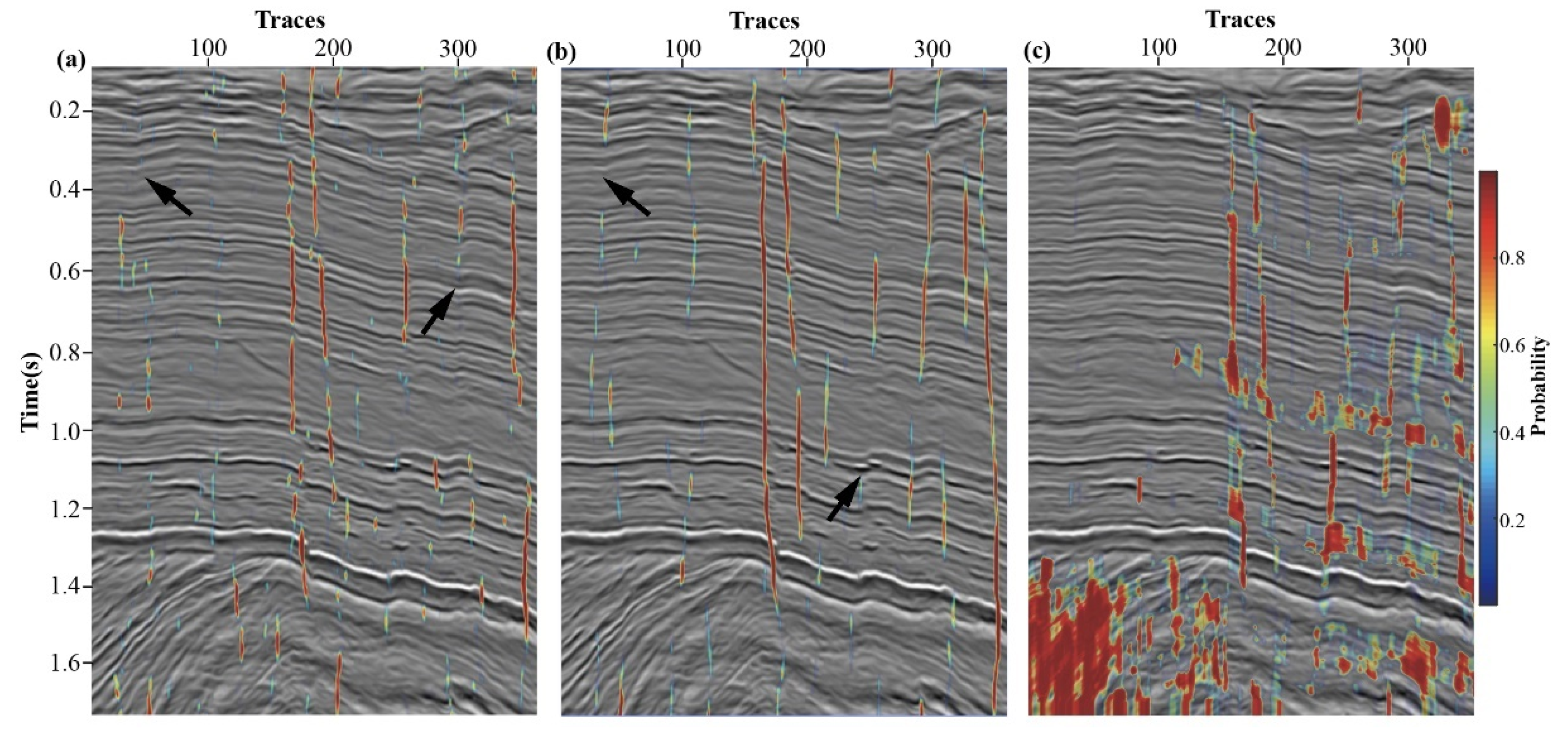
3.2. Comparison of Fault Detection Results with Different Training Samples and Seismic Coherence

The textural features indicated that the generated Kerry3d and Data1 samples were similar to the real Kerry3d and Data1 samples, respectively, and that the generated samples were target-oriented. To verify whether the target-oriented property plays a key role in the application of fault detection, we designed the following comparison experiments. In particular, we used the generated Data1 samples and the merged samples (merging the generated Kerry3d samples and generated Data1 samples) for application and comparison in a section of Kerry3d (same as in Figure 7c). We trained a U-Net using the merged samples, denoted as Net3. Net3 had the same network structure as Net1 and Net2. Then, we used Net2 and Net3 to detect faults in the section shown in Figure 7c. Figure 10a,b show the fault detection results for Net2 and Net 3, respectively. The locations, indicated by the black arrows in Figure 10, show where the fault detection results are not accurate and continuous, while the same locations were accurately marked in Figure 7d. These results demonstrate the importance of target-oriented training samples in fault detection.

Theoretically, the generalization ability of the network can be improved by using more training samples. However, if we use more training samples, it may cause the network more difficult to train. In other words, in practice, it is not always better to have more samples, for example, the Net3, was trained using the merged Kerry and Data1 samples. It theoretically should have better fault detection capability, but the detection result in the Kerry section is no better than Net1. This indicates that target-oriented training samples can be more effective than increasing training samples in some cases.

For objective comparison, we added the results of seismic coherence (Figure 10c). The results display coherence were not continuous and accurate, especially at the locations with low SNR, and Net1 had significantly better detection results than coherence.

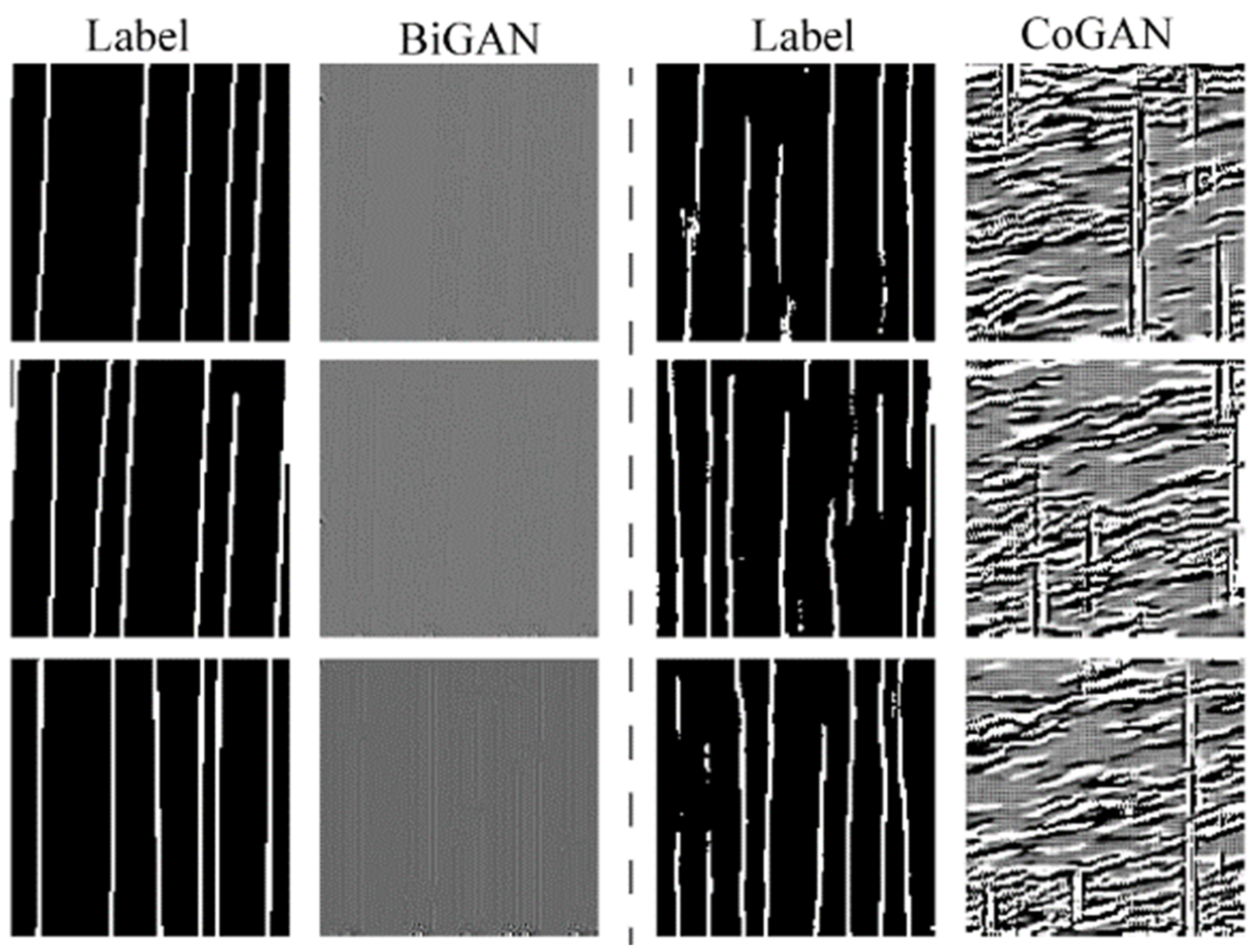
3.3. Comparison of BiGAN and CoGAN Generated Samples

In addition to CycleGAN, bidirectional generative adversarial networks (BiGAN) [37] and coupled generative adversarial network (CoGAN) [38] can also perform unsupervised data generation tasks. We use BiGAN and CoGAN to conduct sample generation experiments on Kerry data. As shown in Figure 11, both BiGAN and CoGAN failed to generate seismic images because the generated images do not have any features of seismic data. Besides, the generated images cannot match the labels. The results show the samples generated by CycleGAN are more realistic compared to BiGAN and CoGAN, and this indicates CycleGAN is more suitable for the task in this paper.

4. Discussion

The seismic fault training samples generated by the proposed label-to-data network achieved favorable results in our experiments, and the generated training samples were shown to be target-oriented. The experimental results indicated that the target-oriented fault training samples could achieve better results than samples that are not target-oriented in relevant applications. For a certain work area, the proposed method can obtain realistic training samples effectively without the need to build seismic structure models according to the features of the work area.

The label-to-data network contains four sub-networks, which means that it consumes a lot of GPU memory. With a sample size of 128 × 128 and batch size of 10, we needed about 4 GB of GPU memory to train the 2D label-to-data network. When we changed the network into the 3D case and set the sample size as 128 × 128 × 128, while keeping the batch size at 10, the required GPU memory can be calculated according to the size of the convolution kernels and feature maps for all layers, which was up to 65 GB. Due to the GPU memory limitations, we did not implement 3D label-to-data networks in the present work.

5. Conclusions

In this paper, we proposed a deep-learning method for obtaining seismic fault training data. This method generates seismic images by learning the features of real seismic data without a need for complex mathematical models or imaging. It solves the problem related to a lack of realistic training data and difficulty in obtaining training data when detecting seismic faults by deep learning. We generated 1000 realistic Kerry and Data1 fault samples with labels using 1000 random labels, and quantitative analysis and experiments demonstrated the reliability of generated data. In addition, this method can generate different target data flexibly according to different work areas. In the future, we intend to focus on generating other seismic structure images, such as those related to seismic caves, salt, and horizons. We also wish to design a lightweight network, to meet the requirements of the 3D situation.

References

1. Bahorich, M.; Farmer, S. 3-D seismic discontinuity for faults and stratigraphic features: The coherence cube. Lead. Edge 1995, 14, 1053–1058. [Google Scholar] [CrossRef]
2. Marfurt, K.J.; Sudhaker, V.; Gersztenkorn, A.; Crawford, K.D.; Nissen, S.E. Coherency calculations in the presence of structural dip. Geophysics 1999, 64, 104–111. [Google Scholar] [CrossRef]
3. Randen, T.; Monsen, E.; Signer, C.; Abrahamsen, A.; Hansen, J.O.; Sæter, T.; Schlaf, J. Three-dimensional texture attributes for seismic data analysis. In SEG Technical Program Expanded Abstracts 2000; Society of Exploration Geophysicists: Houston, TX, USA, 2000; pp. 668–671. [Google Scholar]
4. Gao, D. Integrating 3D seismic curvature and curvature gradient attributes for fracture characterization: Methodologies and interpretational implications. Geophysics 2013, 78, O21–O31. [Google Scholar] [CrossRef]
5. Jing, Z.; Yanqing, Z.; Zhigang, C.; Jianhua, L. Detecting boundary of salt dome in seismic data with edge-detection technique. In SEG Technical Program Expanded Abstracts 2007; Society of Exploration Geophysicists: Houston, TX, USA, 2007; pp. 1392–1396. [Google Scholar]
6. Aqrawi, A.A.; Boe, T.H. Improved fault segmentation using a dip guided and modified 3D Sobel filter. In SEG Technical Program Expanded Abstracts 2011; Society of Exploration Geophysicists: Houston, TX, USA, 2011; pp. 999–1003. [Google Scholar]
7. LeCun, Y.; Kavukcuoglu, K.; Farabet, C. Convolutional networks and applications in vision. In Proceedings of the 2010 IEEE International Symposium on Circuits and Systems, Paris, France, 30 May–2 June 2010; pp. 253–256. [Google Scholar]
8. Zhang, Z.-D.; Alkhalifah, T. Regularized elastic full-waveform inversion using deep learning. Geophysics 2019, 84, R741–R751. [Google Scholar] [CrossRef]
9. Peters, B.; Granek, J.; Haber, E. Multiresolution neural networks for tracking seismic horizons from few training images. Interpretation 2019, 7, SE201–SE213. [Google Scholar] [CrossRef]
10. Wang, B.; Zhang, N.; Lu, W.; Wang, J. Deep-learning-based seismic data interpolation: A preliminary result. Geophysics 2019, 84, V11–V20. [Google Scholar] [CrossRef]
11. Hu, L.; Zheng, X.; Duan, Y.; Yan, X.; Hu, Y.; Zhang, X. First-arrival picking with a U-net convolutional network. Geophysics 2019, 84, U45–U57. [Google Scholar] [CrossRef]
12. Zhu, W.; Mousavi, S.M.; Beroza, G.C. Seismic signal denoising and decomposition using deep neural networks. IEEE Trans. Geosci. Remote Sens. 2019, 57, 9476–9488. [Google Scholar] [CrossRef] [Green Version]
13. Dong, X.; Lin, J.; Lu, S.; Huang, X.; Wang, H.; Li, Y. Seismic shot gather denoising by using a supervised-deep-learning method with weak dependence on real noise data: A solution to the lack of real noise data. Surv. Geophys. 2022, 43, 1363–1394. [Google Scholar] [CrossRef]
14. Iqbal, N. DeepSeg: Deep segmental denoising neural network for seismic data. IEEE Trans. Neural Netw. Learn. Syst. 2022. [Google Scholar] [CrossRef]
15. Wu, X.; Shi, Y.; Fomel, S.; Liang, L. Convolutional neural networks for fault interpretation in seismic images. In SEG Technical Program Expanded Abstracts 2018; Society of Exploration Geophysicists: Houston, TX, USA, 2018; pp. 1946–1950. [Google Scholar]
16. Zheng, Y.; Zhang, Q.; Yusifov, A.; Shi, Y. Applications of supervised deep learning for seismic interpretation and inversion. Lead. Edge 2019, 38, 526–533. [Google Scholar] [CrossRef]
17. Xiong, W.; Ji, X.; Ma, Y.; Wang, Y.; AlBinHassan, N.M.; Ali, M.N.; Luo, Y. Seismic fault detection with convolutional neural network. Geophysics 2018, 83, O97–O103. [Google Scholar] [CrossRef]
18. Di, H.; Shafiq, M.A.; Wang, Z.; AlRegib, G. Improving seismic fault detection by super-attribute-based classification. Interpretation 2019, 7, SE251–SE267. [Google Scholar] [CrossRef]
19. Wu, X.; Liang, L.; Shi, Y.; Fomel, S. FaultSeg3D: Using synthetic data sets to train an end-to-end convolutional neural network for 3D seismic fault segmentation. Geophysics 2019, 84, IM35–IM45. [Google Scholar] [CrossRef]
20. Liu, N.; He, T.; Tian, Y.; Wu, B.; Gao, J.; Xu, Z. Common-azimuth seismic data fault analysis using residual UNet. Interpretation 2020, 8, SM25–SM37. [Google Scholar] [CrossRef]
21. Wu, X.; Geng, Z.; Shi, Y.; Pham, N.; Fomel, S.; Caumon, G. Building realistic structure models to train convolutional neural networks for seismic structural interpretation. Geophysics 2020, 85, WA27–WA39. [Google Scholar] [CrossRef]
22. Cunha, A.; Pochet, A.; Lopes, H.; Gattass, M. Seismic fault detection in real data using transfer learning from a convolutional neural network pre-trained with synthetic seismic data. Comput. Geosci. 2020, 135, 104344. [Google Scholar] [CrossRef]
23. Yan, Z.; Zhang, Z.; Liu, S. Improving performance of seismic fault detection by fine-tuning the convolutional neural network pre-trained with synthetic samples. Energies 2021, 14, 3650. [Google Scholar] [CrossRef]
24. Pan, S.J.; Yang, Q. A survey on transfer learning. IEEE Trans. Knowl. Data Eng. 2009, 22, 1345–1359. [Google Scholar] [CrossRef]
25. Di, H.; Li, C.; Smith, S.; Li, Z.; Abubakar, A. Imposing interpretational constraints on a seismic interpretation convolutional neural network. Geophysics 2021, 86, IM63–IM71. [Google Scholar] [CrossRef]
26. Durall, R.; Tschannen, V.; Ettrich, N.; Keuper, J. Generative models for the transfer of knowledge in seismic interpretation with deep learning. Lead. Edge 2021, 40, 534–542. [Google Scholar] [CrossRef]
27. Ferreira, R.S.; Noce, J.; Oliveira, D.A.; Brazil, E.V. Generating sketch-based synthetic seismic images with generative adversarial networks. IEEE Geosci. Remote Sens. Lett. 2019, 17, 1460–1464. [Google Scholar] [CrossRef]
28. Li, K.; Chen, S.; Hu, G. Seismic labeled data expansion using variational autoencoders. Artif. Intell. Geosci. 2020, 1, 24–30. [Google Scholar] [CrossRef]
29. Feng, Q.; Li, Y.; Wang, H. Intelligent random noise modeling by the improved variational autoencoding method and its application to data augmentation. Geophysics 2021, 86, T19–T31. [Google Scholar] [CrossRef]
30. Zhu, J.-Y.; Park, T.; Isola, P.; Efros, A.A. Unpaired image-to-image translation using cycle-consistent adversarial networks. In Proceedings of the IEEE International Conference on Computer Vision, Venice, Italy, 22–29 October 2017; pp. 2223–2232. [Google Scholar]
31. Ronneberger, O.; Fischer, P.; Brox, T. U-net: Convolutional networks for biomedical image segmentation. In Proceedings of the International Conference on Medical Image Computing and Computer-Assisted Intervention, Munich, Germany, 5–9 October 2015; pp. 234–241. [Google Scholar]
32. Goodfellow, I.; Pouget-Abadie, J.; Mirza, M.; Xu, B.; Warde-Farley, D.; Ozair, S.; Courville, A.; Bengio, Y. Generative adversarial nets. Adv. Neural Inf. Process. Syst. 2014, 27, 139–144. [Google Scholar]
33. Isola, P.; Zhu, J.-Y.; Zhou, T.; Efros, A.A. Image-to-image translation with conditional adversarial networks. In Proceedings of the IEEE Conference on Computer Vision and Pattern Recognition, Honolulu, HI, USA, 21–26 July 2017; pp. 1125–1134. [Google Scholar]
34. Kingma, D.P.; Ba, J. Adam: A method for stochastic optimization. arXiv 2014, arXiv:1412.6980. [Google Scholar]
35. Haralick, R.M.; Shanmugam, K.; Dinstein, I.H. Textural features for image classification. IEEE Trans. Syst. Man Cybern. 1973, 6, 610–621. [Google Scholar] [CrossRef] [Green Version]
36. Kruskal, J.B. Multidimensional scaling by optimizing goodness of fit to a nonmetric hypothesis. Psychometrika 1964, 29, 1–27. [Google Scholar] [CrossRef]
37. Donahue, J.; Krähenbühl, P.; Darrell, T. Adversarial feature learning. arXiv 2016, arXiv:1605.09782. [Google Scholar]
38. Liu, M.-Y.; Tuzel, O. Coupled generative adversarial networks. In Proceedings of the 30th International Conference on Neural Information Processing Systems, Barcelona, Spain, 5–10 December 2016; pp. 469–477. [Google Scholar]
Figure 1. Prepared training samples (column 1 and column 2 are input labels and Kerry faults, and column 4 and column 5 are input labels and Data1 faults, respectively) and expected output (column 3 and column 6).
Remotesensing 15 00265 g001
Figure 2. Label-to-data network structure.
Remotesensing 15 00265 g002
Figure 3. Generator (a) and discriminator (b) structures in the label-to-data networks.
Remotesensing 15 00265 g003
Figure 4. Input labels and output Kerry (a) and Data1 (b) samples (left, binary labels; right, the corresponding fault data).
Remotesensing 15 00265 g004
Figure 5. The average frequency spectra for Kerry (a) and Data1 (c), and the standard deviation of frequency spectra for Kerry (b) and Data1 (d), computed on 1000 samples.
Remotesensing 15 00265 g005
Figure 6. Relative texture dissimilarity of different data sets.
Remotesensing 15 00265 g006
Figure 7. Fault detection test on Kerry3D sections: (a,c) two sections from Kerry 3D; and (b,d) the corresponding prediction results.
Remotesensing 15 00265 g007
Figure 8. Fault detection test on Data1 sections: (a,c) two Inline sections from Data1; and (b,d) the corresponding prediction results.
Remotesensing 15 00265 g008
Figure 9. 3D view of fault detection results for Data1 (a) and Kerry (b).
Remotesensing 15 00265 g009
Figure 10. Comparison of fault detection results on Kerry3d section with Net2 (a), Net3 (b), and seismic coherence (c).
Remotesensing 15 00265 g010
Figure 11. The generated samples of BiGAN (column 2) and CoGAN (column 4).
Remotesensing 15 00265 g011
Disclaimer/Publisher’s Note: The statements, opinions and data contained in all publications are solely those of the individual author(s) and contributor(s) and not of MDPI and/or the editor(s). MDPI and/or the editor(s) disclaim responsibility for any injury to people or property resulting from any ideas, methods, instructions or products referred to in the content.