Article

Hyperspectral Image Super-Resolution Method Based on Spectral Smoothing Prior and Tensor Tubal Row-Sparse Representation

1
School of Computer and Software, Nanjing University of Information Science and Technology (NUIST), Nanjing 210044, China
2
Jiangsu Collaborative Innovation Center of Atmospheric Environment and Equipment Technology (CICAEET), Nanjing University of Information Science and Technology, Nanjing 210044, China
3
Engineering Research Center of Digital Forensics, Ministry of Education, Nanjing University of Information Science and Technology (NUIST), Nanjing 210044, China
4
Henan Key Laboratory of Food Safety Data Intelligence, Zhengzhou University of Light Industry, Zhengzhou 450002, China
*
Author to whom correspondence should be addressed.
Remote Sens. 2022, 14(9), 2142; https://doi.org/10.3390/rs14092142
Submission received: 30 March 2022 / Revised: 25 April 2022 / Accepted: 27 April 2022 / Published: 29 April 2022
(This article belongs to the Section Remote Sensing Image Processing)

Abstract

:
Due to the limited hardware conditions, hyperspectral image (HSI) has a low spatial resolution, while multispectral image (MSI) can gain higher spatial resolution. Therefore, derived from the idea of fusion, we reconstructed HSI with high spatial resolution and spectral resolution from HSI and MSI and put forward an HSI Super-Resolution model based on Spectral Smoothing prior and Tensor tubal row-sparse representation, termed SSTSR. Foremost, nonlocal priors are applied to refine the super-resolution task into reconstructing each nonlocal clustering tensor. Then per nonlocal cluster tensor is decomposed into two sub tensors under the tensor t-prodcut framework, one sub-tensor is called tersor dictionary and the other is called tensor coefficient. Meanwhile, in the process of dictionary learning and sparse coding, spectral smoothing constraint is imposed on the tensor dictionary, and L 1 , 1 , 2 norm based tubal row-sparse regularizer is enforced on the tensor coefficient to enhance the structured sparsity. With this model, the spatial similarity and spectral similarity of the nonlocal cluster tensor are fully utilized. Finally, the alternating direction method of multipliers (ADMM) was employed to optimize the solution of our method. Experiments on three simulated datasets and one real dataset show that our approach is superior to many advanced HSI super-resolution methods.

1. Introduction

Hyperspectral image (HSI), as a three-dimensional data cube with two spatial dimensions and one spectral dimension, contains rich spatial and spectral information of ground objects. Due to this advantage, it has been widely used in many fields such as denoising [1], unmixing [2], classification [3,4], and object detection [5]. However, limited by the hardware conditions of the sensor, there is a trade-off between the spatial resolution and spectral resolution of HSIs. That is, HSIs usually have lower spatial resolution and higher spectral resolution, while multispectral images (MSIs) have lower spectral resolution and higher spatial resolution. Therefore, it is urgent and necessary to fuse the information of HSI and MSI to obtain an HSI with higher spatial and spectral resolutions, thereby improving the accuracy of practical applications.
In recent decades, scholars have proposed many methods for hyperspectral and multispectral fusion. According to the characteristics and theoretical basis of HSI super-resolution, those related work can be divided into four categories: the methods based on pan-sharpening, the methods based on matrix decomposition, the methods based on deep learning, and the methods based on tensor decomposition.

1.1. Fusion Based on Pan-Sharpening

The early fusion method is to fuse the lower-resolution MSI with the higher-resolution panchromatic (PAN) image, called pansharpening. The typical techniques include component projection-substitution (CP) [6] and multiresolution analysis (MRA) [7]. CP methods include intensity hue saturation (IHS) transformation [8], principal component analysis (PCA) transformation [9] and Gram–Schmidt (GS) transformation [10]. The main idea of those methods is to replace the component containing spatial information in PAN image with the same element for MSI. The representative methods based on MRA include wavelet transform [11], Laplacian pyramid (LP) [12]. The main idea is to inject the high-resolution spatial structure particulars of the PAN into the MSI. Inspired by this, many methods extend the pan-sharpening way to HSI and MSI fusion, such as hypersharpening [13,14]. However, If there is a large gap between the spatial resolution of HSIs and MSIs, the fusion results will be accompanied by varying degrees of distortion.

1.2. Fusion Based on Matrix Decomposition

Based on the matrix decomposition, it is assumed that the matrix of a high-resolution HSI (HR-HSI) expanded along spectral dimension can be decomposed into the product of a spectral basis matrix and a coefficient matrix, and the fusion problem is transformed into the estimation of a spectral basis matrix and a coefficient matrix. Specifically, based on the linear mixed spectral model [15], Yokoya et al. [16] proposed a coupled non-negative matrix decomposition method to alternately update the hyperspectral endmember and the abundance matrix with high spatial resolution. Having the idea that there is a strong correlation between bands of an HSI, Simões et al. [17] estimated spectral features in a low-dimensional subspace by using the low-rank feature between bands of the HSI, thus improving the fusion accuracy and efficiency. Similarly, Zhang et al. [18] fully explored the multi-manifold structure and low-rank structure of spectral bands, and proposed an method based on fusion on group spectral embedding (GSE). More recently, the sparse representation methods have shown good capabilities in estimating the spectral basis matrix and coefficient matrix to obtain the desired results. The work of [19,20,21,22,23,24,25,26,27] regarded spectral basis as an overcomplete dictionary to obtain sparsity, and enforced sparsity constraints to the coefficient matrix. Akhtar et al. [19] proposed a Bayesian sparse coding method. Dong et al. [20] proposed a non-negative structure sparse representation method, and utilized the clustering sparsity of HSI for fusion task. Later, Xue et al. [26] proposed a structured sparse representation model by utilizing higher-level spectrum and spatial prior. In general, the premise of matrix decomposition-based methods is to expand HR-MSI and LR-HSI into matrices along spectral dimensions, which often ignore the original structure of hyperspectral images. Although the accuracies are improved compared to pansharpening methods, however, matrix factorization-based methods have higher computational complexity and parameter settings.

1.3. Fusion Based on Deep Learning

In recent years, deep learning has made major breakthroughs in the application of image processing. Dong et al. [28] applied convolutional neural networks (CNN) to image super-resolution for the first time. Since then, a lot of work has been carried out around deep learning methods. For instance, Palsson et al. [29] proposed a 3D convolutional network-based fusion algorithm, which regarded the fusion problem as a spectral super-resolution task of multispectral images. First, the down-sampled multispectral image and the original hyperspectral image were used to learn between the images. Then the learned model was utilized to complete the super-resolution of MSI. Zhang et al. [30] focused more on reconstructing the missing spatial and spectral information of the image, and proposed SSR-NET based on the spatial and spectral edge loss. Yang et al. [31] established a two-branch convolutional neural network architecture to extract multispectral images and hyperspectral images separately, and combine features to achieve super-resolution goals. Compared with traditional machine learning methods that rely on the design of strong handcrafted features, deep learning methods are data-driven, and directly learn prior knowledge from a large amount of data. For example, Wei et al. [32] proposed a deep recursive network based on a deep structure prior and achieved excellent performance. Because the three-dimensional (3D) convolution operation can preserve the spatial-spectral correlation of the HSI better than the one-dimensional (1D) and two-dimensional (2D) convolution operations, Wang et al. [33] proposed to extract spectral and spatial information of source images through 1D convolution and 2D convolution while Hu et al. [34] proposed a multi-scale feature fusion aggregation network based on 3D convolution, which had better reconstruction results. In addition, the non-blind method relies on the fully known point spread function (PSF) and spectral response function (SRF) to simulate the degradation process. Some super-resolution methods based on deep learning can adaptively simulate these two functions. From this perspective, Zheng et al. [35] adaptively learn the parameters of PSF and SRF through two special convolutional layers and a self-encoding network. Inevitably, deep learning methods have some shortcomings. Compared with traditional method models, the neural network used in deep learning is poorly interpretable, and it relies on a large number of data sets for training, also requires high hardware conditions.

1.4. Fusion Based on Tensor Decomposition

Recently, tensor decomposition has rapidly emerged in the fields of high-dimensional image denoising, image completion, and compressed sensing. Since HSIs possess a three-dimensional tensor structure that integrates spatial and spectral information, tensor decomposition has become a hot spot for HSI super-resolution [36]. Li et al. [37] took the lead in applying Tucker decomposition to hyperspectral image fusion, alternately estimating dictionaries of the three modes and a core tensor. In addition, Dian et al. [38] added a non-local prior to estimate each non-local cluster, reducing the computational cost of each iteration, and also discussed the effect of image reconstruction under blind conditions. On this basis, Wan et al. [39] stacked each non-local cluster into a fourth-order tensor and discussed the cluster sparsity. In addition, CANDECOMP/PARAFAC decomposition (CPD) can also capture the dependencies between different dimensions, and Kanatsoulis et al. [40] utilized the coupled CPD model to handle the HSI-MSI fusion task. However, based on the fusion model of Tucker decomposition or CPD, although the size of each modal dictionary is obviously reduced, the interaction between spatial information and spectral information is also weakened by the matrixing operation in the decomposition process. Moreover, the tensor train decomposition model and tensor ring decomposition model have a more vital ability to mine the internal structure of the data. These two decomposition models can effectively maintain the inherent low-rank structure of the tensor while avoiding the loss of original information. For example, Dian et al. [41] applied a regular term to the tensor train decomposition factor and achieved good reconstruction results. Then, Dian et al. [42] proposed a method based on low-rank subspace to estimate the spectral dictionary and coefficients. Later, Xu et al. [43] proposed a non-convex rank constrained fusion model of tensor ring factors, which imposed tensor nuclear norm constraints on decomposition factors. Inspired by t-prodcut based tensor sparse representation [44], Xu et al. [45] proposed a new HSI super-resolution framework. However, the model proposed in [45] lacked some considerations of the inherent properties of HSIs. For example, it did not make full use of the essential characteristics of the tensor decomposition factor and only used the L 1 norm to solve the tensor coefficients, which would lead to loss of primary information and sub-optimal solutions in practical applications. In addition, the model adopted orthogonal constraints on the dictionary tensor, so that the spectrum of the linear combination of these base spectra did not satisfy the smooth property. Therefore, there are still too much room left for improvement.
In this paper, we focus more on the properties of the reconstructed image itself. Combining the characteristics of hyperspectral images, we carefully design the constraints of spectral smoothing and tubal row-sparse on the framework mentioned in [45] and propose a new HSI super-resolution model. In each iteration process, the reconstruction image is made closer to the structural properties of the image itself. The advantages of our method are mainly reflected in two aspects. First, we use a nonlocal patch-wise way to deal with the fusion problem, instead of directly processing it on the whole image. Second, we pay more attention to the internal structure and properties of the tensor factorization. On the one hand, we impose a spectral smoothing constraint on the tensor spectral dictionary, and on the other hand, we impose the L 1 , 1 , 2 norm [46] on the tensor coefficient factor to capture the intrinsic structure of it. Compared with current super-resolution methods, our contributions are as follows.
  • We approach the fusion problem in a patch-wise way instead of directly processing the images. Specifically, to fully exploit the spatial self-similarity of HSI, we use a clustering method on the source image and construct multiple nonlocal tensor patches. On this basis, we apply the tensor sparse representation model to the reconstruction of each nonlocal tensor patch. In this way, the efficiency of our method is improved.
  • Furthermore, based on the tensor sparse representation model, we focus more on the properties of hyperspectral images. To make the reconstructed image closer to the original properties of HSI, we impose a spectral smoothing constraint on the tensor dictionaries to promote the spectral smoothness of reconstructed images. Meanwhile, it was noted that we use the L 1 , 1 , 2 norm [46] to characterize the tubal row-sparsity exhibited by the coefficient tensor.
  • We perform effective convex approximation for each term of the model and use ADMM [47] to optimize the solution of the model. Comparative experiments conducted on multiple simulated data sets and one real data set validate that the proposed method is superior to the current advanced competitors.
The remainder of this paper is organized as follows. Section 2 presents the basic notations with HSI super-resolution problem, as well as some of the related work, and our proposed method. Section 3 presents the optimization algorithm. In Section 4, we show the results of comparing our method with other methods in three simulated data sets and one real data set. In Section 5, we discuss parameter selection and the effectiveness and superiority of our designed constraints. Section 6 presents the conclusions.

2. Materials and Methods

2.1. Notions and Definitions

In this section, we will introduce the symbols and definitions [44] involved in this paper. It is important to note that we use lowercase letters for vectors, capital letters for matrices, and Euler Script letters for tensors.
Definition 1
(Mode-n unfolding). The mode-n unfolding matrix of the P-dimensional tensor X     R f 1 × f 2 × × f P is denoted as X ( p )     R f p × f 1 f 2 , , f p 1 f p + 1 , , f P , which is also represented by u n f o l d p ( X )   =   X ( p ) , and  X   =   f o l d p ( X ( p ) ) . It takes the n t h dimension fiber as the column of the matrix, mapping the tensor elements into the matrix elements. Noted that X ( : , i , j ) , X ( i , : , j ) and X ( i , j , : ) are the column, row, and tubal fibers of X , respectively.
Definition 2
(Mode-n Tensor-Matrix Product). The mode-n tensor-matrix product of a tensor X     R I 1 × I 2 × × I N and a matrix A     R P n × I n is a tensor Y     R I 1 × I 2 × × I n 1 × P n × I n + 1 × × I N denoted by X × k A and its elements are computed by
X × k A i 1 , , i k 1 , j , i k + 1 , , i N   =   i k x i 1 i k 1 i k i k + 1 i N a p n i n
Here, we have Y   =   X × k A Y ( k )   =   A X ( k ) .
Definition 3
(t-prodcut). The t-prodcut between D     R d 1 × d 2 × d 3 and A     R d 2 × d 4 × d 3 is J     R d 1 × d 4 × d 3 , where J ( i , j , : )   =   m = 1 r D ( i , m , : )     A ( m , j , : ) , and ∗ represents a circular convolution operator. To better understand, we represent the t-prodcut using the following operator. First, we use D ( i ) to represent D ( : , : , i ) , i     d 3 , each D ( i ) is a frontal slice of D . Then, we define the block circular matrix blkcirc ( D )     R d 1 d 3 × d 2 d 3 as
blkcirc ( D )   =   D ( 1 ) D d 3 D ( 2 ) D ( 2 ) D ( 1 ) D d 3 D d 3 D d 3 1 D ( 1 )
Next, we define the operator of unfolding and folding of the frontal slices of D as
U n f o l d V ( D )   =   D ( 1 ) D ( 2 ) D d 3 , F o l d V U n f o l d V ( D )   =   D
At this point, the t-prodcut between D and A is J   =   D A   =   Fold V b l k circ ( D ) ·
Unfold V ( A )     R d 1 × d 4 × d 3 . To solve the tensor-tensor product optimization problem quickly, we introduce a significant tool called the Discrete Fourier Transform (DFT). Let D ¯     R d 1 × d 2 × d 3 represents transformation form of DFT of D     R d 1 × d 2 × d 3 along the 3rd mode, we define D ¯     R d 1 d 3 × d 2 d 3 as follows:
D ¯   =   blockdiag ( D ¯ )   =   D ¯ ( 1 ) D ¯ ( 2 ) D ¯ d 3
The function of blockdiag ( · ) operator above is mapping the tensor D ¯ to the block matrix arranged diagonally. Then we will use the following Lemma to explain why we can use DFT to solve our problem quickly.
Lemma 1
([48]). Assume that D     R d 1 × d 2 × d 3 , A     R d 2 × d 4 × d 3 are two random tensors. Let J   =   D     A . Then, we introduce the theorem of property as follows.
  • J F 2   =   1 d 3 J ¯ F 2
  • J   =   D A is equivalent to J ¯   =   D ¯ A ¯ , thus, we have J ¯ ( j )   =   D ¯ ( j ) A ¯ ( j ) , j [ d 3 ]
Definition 4
( L 1 , 1 , 2 norm and tubal row-sparsity). For a tensor A     R d 1 × d 2 × d 3 , we define A ( i , j , : ) as a tube of A , and define the tubal row-sparse of A as the number of non-zero tubes of A . Here, we use L 1 , 1 , 2 norm to compute the tubal sparsity [49]. The definition of L 1 , 1 , 2 norm is given as follows.
A 1 , 1 , 2   =   i , j A ( i , j , : ) F
which calculates the summation of the L 2 norm of all tubes of A .

2.2. Preliminaries

2.2.1. Problem Formulation

To facilitate understanding, we build a preliminary observation model, and use Euler Script letters to represent two input images and one output image, respectively.
Through the fusion of LR-HSI Y     R w × h × C and HR-MSI Z     R W × H × c , we obtain the target image HR-HSI X     R W × H × C , where W, w and H, h represent the dimensions of the spatial width and height, respectively. C and c represent the dimension of the spectral. It is noted that w < < W , h < < H and c < < C . As mentioned at Definition 1, X ( 3 )     R C × W H , Y ( 3 )     R C × w h , and  Z ( 3 )     R c × W H indicate matrices of X     R W × H × C , Y     R w × h × C and Z     R W × H × c expanded along spectral mode individually. Therefore, we establish a preliminary representation relationship.
Y ( 3 )   =   X ( 3 ) B H   +   N h s
Z ( 3 )   =   R X ( 3 )   +   N m s
where B     R W H × W H represents the spatial blurring operator and H     R W H × w h is often assumed to be a down-sampling matrix. N h s represents the independent and identically distributed (i.i.d.) noise of LR-HSI. R     R c × C represents the spectral response of multispectral sensor. N m s indicates the independent and identically distributed (i.i.d.) noise of HR-MSI.
Based on the above description, we build a preliminary model as follows.
arg min X ( 3 ) 1 2 Y ( 3 )     X ( 3 ) B H F 2   +   δ 2 Z ( 3 )     R X ( 3 ) F 2   +   λ ϕ X ( 3 )
where δ is a parameter that measures the relationship between the two fidelity terms. There may be multiple solutions to solve this problem, resulting in severely ill-posed of the problem. Therefore, we carry out appropriate regularization constraints on the problem according to the prior knowledge of hyperspectral images. ϕ X ( 3 ) represents the constraint on the spatial and spectral information of potential X ( 3 ) and λ represents the coefficient of the constraint term.

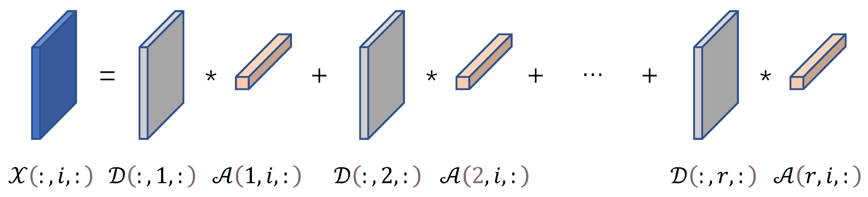
2.2.2. Tensor Sparse Representation Based on t-Product

Because of the similarity and redundancy between the bands of hyperspectral data, sparse representation has a strong advantage in super-resolution reconstruction model. For high-dimensional image data, traditional methods based on matrix decomposition usually embed high-dimensional data into the matrix space and use traditional dictionary learning methods to complete restoration or denoising tasks. However, this matrixization will break the original multi-dimensional structure of the image, Zhang et al. [46] proposed the tensor dictionary learning and considered the sparsity of the tensor coefficient based on the t-prodcut mentioned in Definition 3, and offered a tensor combination sparse representation model. The model is as follows.
arg min D , A 1 2 X     D A F 2   +   λ A 1
where X     R a × n × b indicates a third-order tensor which is stacked by n images of size a × b . D     R a × r × b represents a dictionary which also is a third-order tensor and per lateral slice of the dictionary indicates an atom. So, r expresses the number of atoms. A     R r × n × b represents the tensor sparse coefficients. λ is a sparse regularization parameter. According to the algebraic form of tensor-tensor product, each lateral slice of X     R a × n × b can be linearly combined by tensor dictionary and tensor coefficient. Here, we present a linear combination representation of each lateral slice below as shown in Figure 1.
X ( : , i , : )   =   D   ×   A ( : , i , : )   =   D ( : , 1 , : )   ×   A ( 1 , i , : )   +     +   D ( : , r , : )   ×   A ( r , i , : )

2.3. Proposed Method

Given the tensor linear combination sparse representation model based on t-prodcut, we proposed a super-resolution method based on this model. To take full advantage of the nonlocal self-similarity of hyperspectral images, we first performed nonlocal clustering on the up-sampled LR-HSI and HR-MSI, and transformed the problem into the reconstruction of each cluster of HR-HSI. Then per nonlocal cluster tensor was decomposed into two sub tensors under the tensor t-prodcut framework, and the potential properties of each sub tensor were explored. Specifically, the tensor dictionary was constrained by the prior knowledge of spectral smoothing (spectrum continuity) of HSIs. In addition, the  L 1 , 1 , 2 norm was utilized to well characterize the tubal-row sparsity of tensor coefficients. Finally, the ADMM algorithm was employed to iteratively solve our model. The flowchart of the proposed method is shown in Figure 2.

2.3.1. Nonlocal Cluster Tensor

To capture strong low rankness of the patches in HSIs, we incorporate a nonlocal self-similarity prior to the model. Briefly, we divide the image into multiple patches by a clustering algorithm and stack these patches with similar spectral and spatail features into clusters. That is, we change the super-resolution task of the whole image into the reconstruction of each cluster. Here, we employ [49] to sort all the segmented patches into a highly smooth one-dimensional sequence, in which the two adjacent patches are highly similar. All you need to do is initializing the number of each cluster on the sequence.
Since HR-HSI is unknown, we cannot group it directly. Therefore, we cluster and group HR-HSI based on the spatial information and location of HR-MSI. So we first divide HR-MSI Z     R W × H × c into a group of overlapping tensor patches J i 1 < i < N     R v w × v h × c , where v w and v h indicate the width and height of the patch of the partitioning tensor, and N represents the number of patches of all the partitioning blocks. Then we group these tensor patches to form multiple clusters. The elements of per cluster are tensor patches with dimension of v w   ×   v h   ×   c . We use J i k 1 < i < n     R v w × v h × c to represent the k t h cluster with n tensor patches. Then, we expand each element of each cluster into a matrix along the spectral dimension of the tensor, and stack each matrix to form a new third-order tensor. We use Z k     R c × v w v h × m k to represent this new third-order tensor, and we have Z k ( : , : , i )   =   unfold 3 J i k . Finally, we rewrite the fusion problems with the tensor notions as follows.
arg min X 1 2 Y     X B H F 2   +   δ 2 Z     R X F 2 s . t . Y   =   k U k T U k 1 k U k T Y k Z   =   k U k T U k 1 k U k T Z k
Here, U k represents the operator that extracts the k t h nonlocal cluster tensor from HR-MSI or LR-HSI, that is, Z k   =   U k Z , Y k   =   U k Y . B and H represent spatial blurring kernel and downsampling operator, respectively. However, in practice, we use mode-n tensor-matrix product for computation, where X B H is equivalent to B H X ( 3 ) . In addition, each pixel intensity of HR-MSI is equal to the spectral response times the pixel intensity in the corresponding HR-HSI. So when we use t-product to compute Z   =   R X , we have Z k ( i )   =   R X k ( i ) , i   =   1 , , m k to compute each slice individually, as shown in the following equation.
Z k ( 1 ) Z k ( 2 ) Z k m k   =   R 0 0 0 R 0 0 0 R X k ( 1 ) X k ( 2 ) X k m k

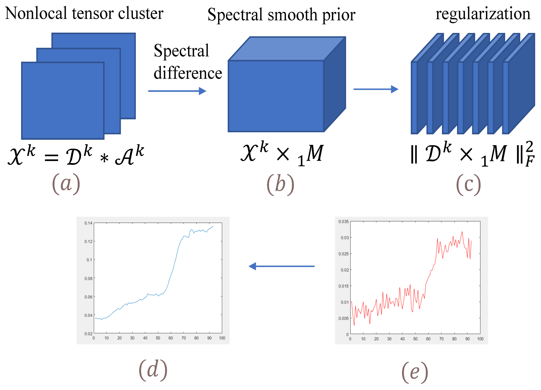
2.3.2. Spectral Smooth Prior on Nonlocal Cluster Tensor

In HSIs, the nonlocal similarity between different patches not only represents the spatial structure similarity, but also represents spectral similarity. So, we apply t-prodcut to the reconstruction process of nonlocal cluster tensor. In this case, similar patches are likely to belong to the same type of ground material at the same coordinates, so they should be represented on the same basis. Based on Section 2.2.2, each nonlocal cluster tensor is reconstructed separately as follows.
arg min X , D k , A k 1 2 Y     X B H F 2   +   k = 1 K δ 2 Z k     R     D k     A k   +   λ A k 1 s . t . Z   =   k U k T U k 1 k U k T Z k
For each nonlocal cluster tensor X , we have to estimate two sub tensors: tensor dictionary D k and coefficient tensor A k . In this section, we only discuss the properties of tensor dictionary. From Equation (10), it is easy to find that each lateral slice of the tensor is a linear combination of the corresponding tensor dictionary D k and coefficient tensor A k . This means that these lateral slices can be regarded as the basis of the spectral space D k . That is, continuous bases tend to generate continuous data. For hyperspectral data, spectral smoothing is an important property. We assume that if we enforce the spectrum of each base of the dictionary to be smooth enough, then the spectrum of the nonlocal cluster tensor reconstructed from these bases will also be smooth enough. To confirm this hypothesis, we reconstructed one nonlocal cluster tensor by applying spectral smoothing constraint and without applying spectral smoothing constraint, respectively. From Figure 3, there are obvious differences between the spectral curves at the same spatial location, the original curve shows a smooth change. Therefore, we impose spectral smoothing constraints on tensor dictionary for all nonlocal cluster tensors. Then, (13) can be rewritten as follows.
arg min X , D k , A k 1 2 Y     X B H F 2   +   k = 1 K δ 2 Z k     R     D k     A k   +   τ D k   ×   1 M F 2   +   λ A k 1 s . t . Z   =   k U k T U k 1 k U k T Z k
where M represents a first-order difference matrix, τ is a regularization parameter and × k is the k-mode product between tensor and matrix.

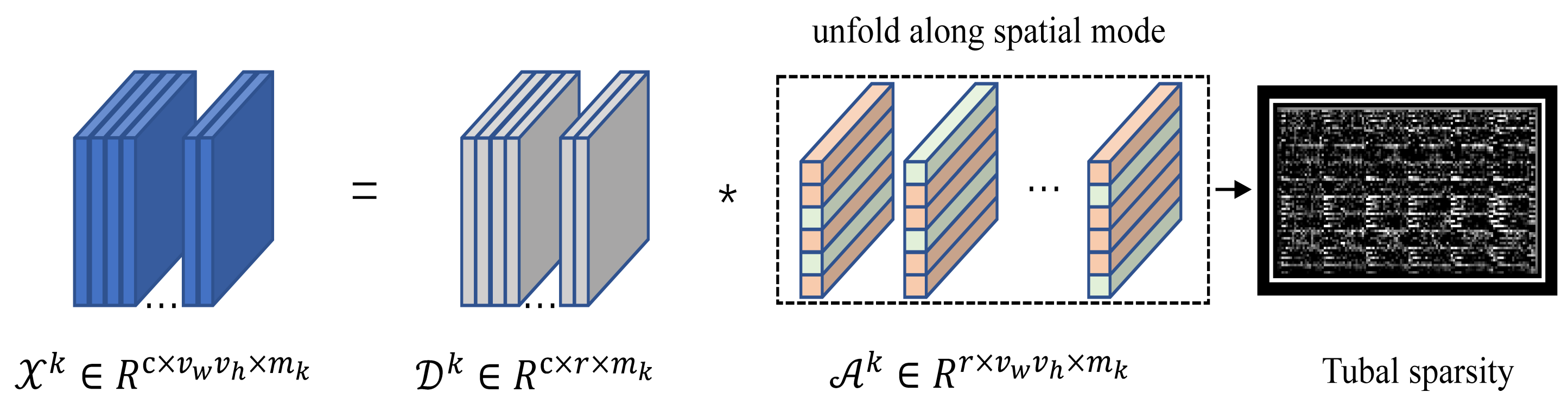
2.3.3. Tubal Sparsity Constraint with Sparse Representation Model for Nonlocal Cluster Tensor

Since the optimization problem of L 0 norm is not convex [50], many scholars proposed to use a convex relaxation technique to transform it into a convex optimization problem. Xu’s work [45], as well as Li’s [37] and Dian’s [38] work, only uses L 1 norm [51] to constrain the tensor coefficients. However, it ignores the underlying structural properties of tensor coefficient factors, which can easily lead to loss of image information and sub-optimal solutions. Therefore, we explore the intrinsic structural properties of tensor coefficients from two aspects. On the one hand, based on tensor sparse representation model of t-prodcut, the actual operation is the convolution operation between the lateral slices of the tensor dictionary and tubes of the tensor coefficients. Therefore, we reckon that it is easier to obtain an optimal solution by capturing the sparsity presented by all tubes of the tensor coefficient. On the other hand, the group sparse signals are more seemly to emerge after nonlocal clustering than completely random sparse signals. As illustrated in Figure 4, the tensor coefficients exhibit a row sparsity. So, we use the L 1 , 1 , 2 norm mentioned in Definition 4 to characterize the tubal row-sparsity of tensor coefficients.
So, we rewrite Equation (14) as follows.
arg min X , D k , A k 1 2 Y     X B H F 2   +   k = 1 K δ 2 Z k     R     D k     A k   +   τ D k   ×   1 M F 2   +   λ W k     A k 1 , 1 , 2 s . t . Z   =   k U k T U k 1 k U k T Z k
where W k represents a weight tensor that better promote the tubal sparsity, and ⊙ represents the operation of component-wise multiplication.

3. Optimization Algorithm

Having ADMM algorithm in mind, we introduce two new variables to decouple D and A , so we can express (14) as the following Lagrangian.
L X = 1 2 Y     X B H F 2   +   k = 1 K δ 2 Z k     R     D k     A k F 2   +   λ W k E k 1 , 1 , 2   +   τ C k   ×   1 M F 2 + k = 1 K P 2 k , D k     C k   +   σ 2 k = 1 K D k     C k F 2 +   k = 1 K P 3 k , A k     E k   +   σ 2 k = 1 K A k     E k F 2 + P 1 , X     k = 1 K U k T U k 1 k = 1 K U k T D k     A k + σ 2 X     k = 1 K U k T U k 1 k = 1 K U k T D k     A k F 2
where P 1 , P 2 k , and  P 3 k are the so-called Lagrange multipliers, σ is a penalty parameter. Then we solve this optimization algorithm by alternatively updating each variable with the others fixed. It should be noted that each cluster tensor is optimized and solved separately, and  C k , D k , E k and A k are all updated independently. The optimization process is as follows.
 (1)
Update C k
arg min C k σ 2 C k     D k     P 2 k / σ F 2   +   τ C k   ×   1 M F 2
In order to facilitate the solution, the tensors in the equation are expanded along 1     m o d e . The optimal of C k along 1     m o d e is
C ( 1 ) k   =   σ I   +   τ M T M 1 σ D ( 1 ) k   +   P 2 k
It is worth noting that D ( 1 ) k and P 2 k are the unfolded matrices of C k and P 2 k along the first dimension, respectively. After getting C ( 1 ) k , we fold it to tensor form, where C k   =   fold 1 C ( 1 ) k .
 (2)
Update D k
arg min D k δ 2 Z k     R     D k     A k F 2   +   σ 2 X k     D k     A k   +   P 1 k / σ F 2 + σ 2 D k     C k   +   P 2 k / σ F 2
Each D k can be solved seperately. In this case, P 1 k   =   U k P 1 . According to Lemma 1, we know that D k     A k is equivalent to D k ¯ ( i ) A k ¯ ( i ) , i     [ m k ] . Therefore, Equation (19) can be effectively solved in Fourier domain. Its unique solution is equivalent to solving the general Sylvester Equation (20).
δ R ¯ ( i ) R ¯ ( i ) T   +   σ I D k ¯ ( i ) A k ¯ ( i ) A k ¯ ( i ) T   +   σ D k ¯ ( i ) =   δ Z k ¯ ( i ) R ¯ ( i ) A k ¯ ( i ) T   +   σ X k ¯ ( i ) A k ¯ ( i ) T   +   P 1 k ¯ ( i ) A k ¯ ( i ) T   +   σ C k ¯ ( i ) P 2 k ¯ ( i )
The conjugate gradient method [52] is used to solve (20) efficiently.
 (3)
Update E k
The optimization problem of E k is
arg min E k σ 2 E k     A k     P 3 k / σ F 2   +   λ W k     E k 1 , 1 , 2
Here, we use a soft threshold operator for the solution.
E k ( i , j , : )   =   shrink 1 , 1 , 2 temp A k ( i , j , : ) , W k ( i , j )   ·   λ σ
where
temp A k   =   A k   +   P 3 k / σ W k ( i , j )   =   1 temp A k ( i , j , : ) 2   +   γ
If ψ < x 2 , shrink 1 , 1 , 2 ( x , ψ )   =   x 2 ψ x 2 x , otherwise shrink 1 , 1 , 2 ( x , ψ )   =   0 . The function of γ is to avoid singularities.
 (4)
Update A k
The optimization for the coefficient tensors is shown below.
arg min A k δ 2 Z k     R     D k     A k F 2   +   σ 2 X k     D k     A k   + P 1 k / σ F 2   +   σ 2 A k     E k     P 3 k / σ F 2
Similar to D k , A k can be effectively solved in the Fourier domain.
A k ¯ ( i )   =   δ D k ¯ ( i ) T R ¯ ( i ) T R ¯ ( i ) D k ¯ ( i )   +   σ D k ¯ ( i ) T D k ¯ ( i ) 1 δ D k ¯ ( i ) T R ¯ ( i ) T Z k ¯ ( i )   +   σ D k ¯ ( i ) T X k ¯ ( i )   +   D k ¯ ( i ) T P 1 k ¯ ( i )   +   σ E k     P 3 k ( i )
 (5)
Update X
The optimization problem of X is
X   =   arg min X 1 2 Y     X B H F 2   +   P 1 , X     k = 1 K U k T U k 1 k = 1 K U k T D k     A k +   σ 2 X     k = 1 K U k T U k 1 k = 1 K U k T D k     A k F 2
Here, we convert it to
X B H H T B T   +   σ D )   =   Y H T B T     P 1   +   σ k = 1 K U k T U k 1 k = 1 K U k T D k     A k
Here, we use the conjugate gradient method to solve (27) efficiently.
 (6)
Update Lagrange multipliers
P 1   =   P 1   +   σ X     k = 1 K U k T U k 1 k = 1 K U k T D k A k P 2 k   =   P 2 k   +   σ D k     C k , k = 1 , K P 3 k   =   P 3 k   +   σ C k     E k , k = 1 , K
where σ   =   s σ , s > 1 and the process of SSTSR is shown in Algorithm 1.
Algorithm 1 The proposed SSTSR method for HSI super-resolution.
  • Require: LR-HSI Y , HR-MSI Z , v w , v h , B , R , H , δ , λ , τ
  • Ensure: HR-HSI X ( i )
1:
Initialization: i   =   1 , i m a x   =   15 , X ( 0 )   =   Y H T B T , P 1 ( 0 )   =   0 , P 2 ( 0 ) k   =   0 , P 3 ( 0 ) k   =   0 , D ( 0 ) k , A ( 0 ) k , C ( 0 ) k , E ( 0 ) k are randomly initialized with the scale dimensions, σ   =   1 , s   =   1.01 , tol=0.001.
2:
While not converged and i   <   i m a x  do
3:
For c l u s t e r k   =   1 : M a x k
4:
Update E ( i ) k by (22)
5:
Update C ( i ) k by (18)
6:
Update D ( i ) k by (20) with CG
7:
Update A ( i ) k by (25)
8:
Update P 2 ( i ) k , P 3 ( i ) k by (28)
9:
End for
10:
Update X ( i ) by (27) with CG
11:
Update P 1 ( i ) by (28), σ   =   s σ
12:
Check the convergence condition
13:
X ( i )     k = 1 K U k T U k 1 k = 1 K U k T D ( i ) k A ( i ) k F 2 <tol, X ( i )     X ( i 1 ) F 2 <tol
14:
k = 1 K U k T U k 1 k = 1 K U k T D ( i ) k A ( i ) k k = 1 K U k T U k 1 k = 1 K U k T D ( i 1 ) k     A ( i 1 ) k F 2
15:
<tol
16:
Update iteration
17:
i   =   i   +   1
18:
End While

4. Results

4.1. Synthetic Dataset

Data set 1: The first data (http://www.ehu.eus/ccwintco/index.php/Hyperspectral_Remote_Sensing_Scenes, accessed on 29 January 2022) set was formed by ROSIS sensor capturing scenes from the University of Pavia (PU) over northern Italy. The initial data size was 610   ×   340   ×   115 , but considering the presence of water vapor absorption bands in the data and in order to show more spatial details, we sampled the data as the reference image, which has size of 300   ×   300   ×   103 . We simulated LR-HSI by using a 9   ×   9 Gaussian filter with standard deviation 2.12 to blur it from the reference image, then we sampled it with down sampling ratio of 5. We used the spectral response function of IKONOS multispectral sensor to simulate the generation of HR-MSI. After that, the independent identically distributed noise of corresponding SNR was applied. For LR-HSI, the SNR was set to 30 dB, and for HR-MSI, the SNR was arranged to 40 dB.
Data set 2: The second data set (https://engineering.purdue.edu/~biehl/MultiSpec/hyperspectral.html, accessed on 29 January 2022) was formed by HYDICE sensor capturing scenes from the National Mall over Washington, D.C (WDC). Similarly, there were bands with low SNR in this data, so the final size left was 1280   ×   307   ×   191 , and then we chose 300   ×   300   ×   191 as the reference image. We used the same simulation process as the first data set to generate LR-HSI and HR-MSI.
Data set 3: The last data set (2013 IEEE GRSS Data Fusion Contest: http://www.grss-ieee.org/community/technical-committees/data-fusion, accessed on 29 January 2022) was Houston (HOS) captured by ITRES CASI-1500 sensor, which was offered by the 2013 IEEE GRSS Data Fusion Competition. The original size of Houston was 349   ×   1905   ×   144 . Similarly, we selected the bands and sampled the data with rich details of features. So, the final size of reference image was 300   ×   300   ×   103 . We used the same method to generate LR-HSI together with HR-MSI as we did for the first data set.

4.2. Quantitative Metrics

We used six quantitative index [53] to judge our superresolution output.
(1) PSNR: The Peak Signal to-Noise Ratio. PSNR is the most regular objective evaluation index of images and the larger PSNR is, the less image distortion is. Since the data are hyperspectral images with multiple bands, we calculate the average PSNR of all bands.
(2) SAM: The spectral angle mapper. Sam computes the average angle between the estimated image spectrum and the reference image spectrum.
(3) CC: The Correlation Coefficient.
(4) ERGAS: The relative dimensionless global error in synthesis. ERGAS mainly evaluates the spectral quality of all fusion bands.
(5) SSIM: Structural Similarity. It mainly measures the similarity of the estimated image and reference image.
(6) UIQI: The Universal Image Quality Index. The UIQI calculates the average value of all image patches for the estimated image and reference image.

4.3. Compared Methods

We choose some classical and recent advanced methods based on tensor decomposition to compare with our proposed method, including Hysure [17], CSTF [37], NPTSR [45], LTTR [41], NLSTF [38] and LTMR [42]. The parameters of these comparison algorithms are the best parameters described in the reference literature as far as possible.
All methods except for CSTF have the same spectral response function and spatial blur kernels in the experiments. For CSTF, we follow the assumption about the separability of the downsampling operator along spatial modes.
For the parameters used in the comparison algorithms, we follow the reference literature as much as possible, and have adjusted them appropriately. For Hysure, the number of subspace bands is 10 and the dimensions of estimated method choose VCA, λ m   =   1 , λ ϕ   =   5 × 10 4 . For CSTF, n w   =   n h   =   500 , n s   =   15 , λ   =   10 5 . For LTMR, K   =   200 , p a t c h s i z e   =   10 , L   =   10 , λ   =   10 3 . For NLSTF, n w   =   n h   =   10 , n s   =   10 , K   =   150 , λ   =   10 7 , λ 1   =   10 4 , λ 2   =   λ 3   =   10 5 . For LTTR, K   =   460 , λ   =   4 × 10 4 . For NPTSR, λ   =   10 3 , β   =   10 3 , N k   =   3 , r   =   10 .
In addition, we also compare the proposed SSTSR method with the two deep learning methods, i.e., HAM-MFN [54] and CNN-Fus [55], the details are described in Section 4.4.

4.4. Experimental Results on Synthetic Datasets

In this section, we present the results generated by all methods on three simulated datasets, i.e., PU, WDC, and HOS. We also show the comparison of quantitative indicators in Table 1 and Table 2, where the best values are boldface. In addition, we demonstrate the superiority of our method in the following three aspects.
(1)
Visual effects of reconstructed images. Figure 5, Figure 6 and Figure 7 list the fusion results of different methods on three datasets, i.e., PU, WDC, and HOS, respectively. To deepen the visual effect, we pseudo-color the experimental results while magnifying the representative local information. In addition, with the aid of ground truth, the comparison of residual images is supplemented, in which the dark blue residual image indicates better reconstruction effect. As can be seen from Figure 5, Figure 6 and Figure 7, the results of CSTF, LTMR, LTTR, and NLSTF all show color distortion compared with the ground truth. From the residual image, the result of our method is bluer and smoother. It fully verifies that our proposed method can obtain images with better spatial structure details.
(2)
Spectral curve and spectral curve residual. In addition, we also compare the spectral quality of the reconstructed images. Figure 8a shows the spectral curve of the reconstructed image at pixel (90, 90) of the PU dataset and the residual spectral curve of the reconstructed image with the ground truth. Similarly, Figure 8b,c also compare the spectral curves at the pixel (100, 200) of the WDC and the pixel (100, 100) of the HOS, respectively. It is clear from Figure 8 that the spectral curves of the reconstructed images of our method on the three datasets are closer to the ground truth spectral curves, and the residual curves are also closer to the zero-horizontal line. This also demonstrates the effectiveness of the spectral smoothing constraints imposed in our method. Compared with other methods, our proposed SSTSR method can obtain images with higher spectral quality.
(3)
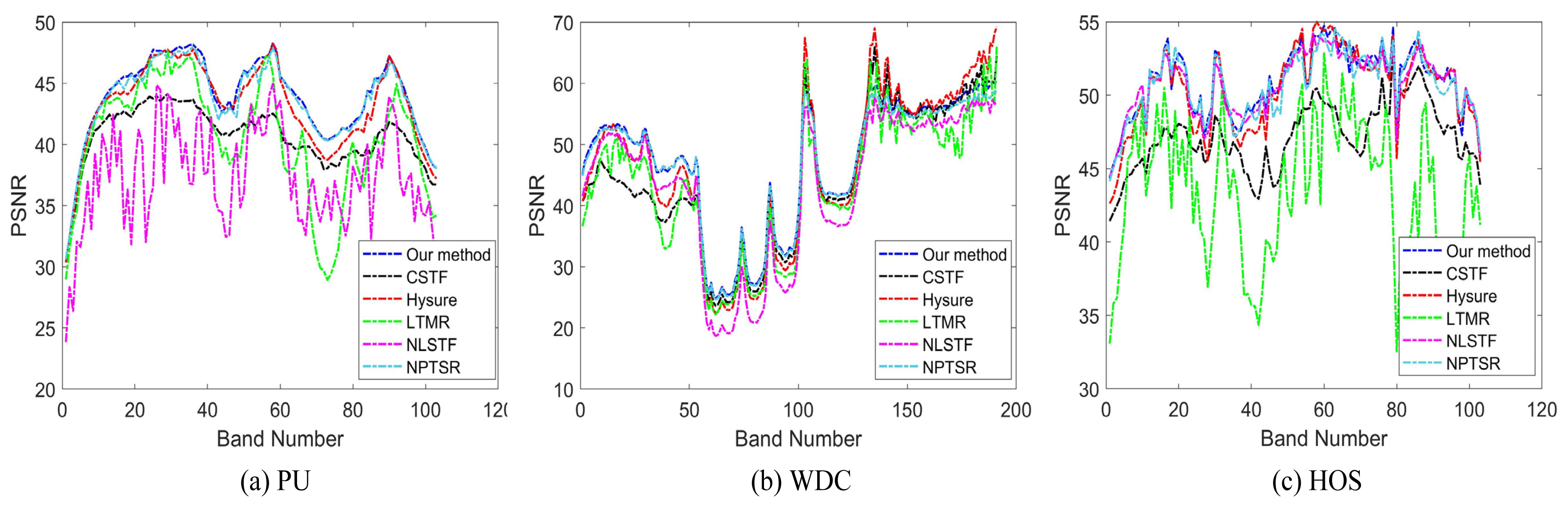
Quantitative indicators and time complexity comparison. As can be seen from Table 1, on the PU dataset, our method achieves a leading position in all indicators, and on the WDC dataset, although the three indicators of SAM, CC, and ERGAS slightly lag behind Hysure and NPTSR, our PSNR, SSIM, UIQI values are still leading, and on the HOS dataset, all indicators of our method once again rank first. It needs to be mentioned that all methods have similar SSIM values on HOS dataset, so the results of this indicator are not listed. Taken together, the average PSNR of our method on the three datasets is 0.63 dB, 2.85 dB, 4.53 dB, 9.84 dB, 2.33 dB, 0.33 dB higher than Hysure, CSTF, LTMR, LTTR, NLSTF, NPTSR, respectively, which verifies the superiority of our method. In addition, we also give a comparison of PSNR in each band for all methods on the three datasets in Figure 9. As can be seen from Figure 9, our method outperforms other methods in most bands. Besides, the measurement of the ERGAS index indicates the spectral quality of the reconstructed image and the smaller the value, the better the spectral quality. The ERGAS value of our method is also state-of-the-art on three datasets. Although the designed regular terms can improve the performance of the method, they also consume more computing time. Our method has no advantage in the comparison of time complexity, so in future work, we will focus on optimizing our method to reduce the time complexity.
We also selected two deep learning methods [54,55] for comparison. Unfortunately, there was a lack of relevant codes. We directly quoted the results in the reference literature for quantitative comparison. For a fair comparison, we set the same conditions for the experiments. (1) The size and scope of HR-HSI and HR-MSI were the same. (2) We simulated and generated LR-HSI and HR-MSI according to the spatial-spectral degradation method described in the reference literature. (3) We selected the same quantitative indicator function. Specifically, compared with the HAM-MFN [54], the selected PU size was 260   ×   340   ×   103 , the upper left corner coordinate was (351, 1), the spectral degradation was simulated by the randomly generated spectral response function, and the spatial degradation was simulated by bicubic linear interpolation and the downsampling ratio was 4. Compared with the CNN-Fus [55], the selected PU size was 610   ×   340   ×   103 , the upper left corner coordinate was (0, 0), the spectral degradation was simulated by the spectral response function of the IKONOS sensor to generate HR-MSI, and the 7   ×   7 Gaussian filter with a standard deviation of 2 was used to simulate spatial degradation with a downsampling ratio of 4. As can be seen from Table 2, our method also showed certain advantages.
Table 1. Quantitative and complexity comparison in simulated PU, WDC and HOS data sets.
DatasetIndexBest ValuesHysure [17]CSTF    [37]LTMR [42]LTTR [41]NLSTF [38]NPTSR [45]SSTSR
PUPSNR+43.2640.7640.7135.5340.7043.5543.84
SAM02.59712.71893.75905.63042.88112.41492.4080
CC10.99460.99430.98680.97690.99150.99500.9951
ERGAS01.15191.20621.60032.39861.54211.12481.1071
SSIM10.93790.93080.90530.82610.93900.94380.9444
UIQI10.92570.91650.88960.80170.92710.93280.9335
TIME0433722017620280371
WDCPSNR+46.0544.6443.3236.7743.2846.4346.81
SAM06.63066.01776.84588.298910.54585.00795.0167
CC10.91770.91150.84170.65800.81670.90970.9150
ERGAS05.71057.453112.633330.802410.64219.03996.4304
SSIM10.73020.66520.55950.35640.64510.75760.7703
UIQI10.67970.71130.50060.32890.61050.71920.7286
TIME0434821035225489673
HOSPSNR+50.2447.1943.8139.6350.4650.4950.80
SAM01.41101.27613.48905.18021.37031.29141.2746
CC10.99800.99810.98900.97790.99820.99820.9983
ERGAS00.67270.64371.74942.29880.62460.61730.6111
SSIM1-------
UIQI10.98190.98100.92890.85620.98310.98380.9835
TIME043358017425271341
Table 2. Comparison of quantitative indicators between the proposed method and the deep learning methods.
DatasetMethodPSNRSAMERGASSSIM
PU (260 × 340 × 103)HAMMFN [54]40.86322.53081.80520.9776
SSTSR44.07462.36271.11560.9428
DatasetMethodPSNRSAMUIQISSIM
PU (610 × 340 × 103)CNN-Fus [55]43.01702.23500.99200.9870
SSTSR43.69802.41490.99320.9607
Table 3. The necessity of using spectral smooth and tubal row-sparse constraints.
ConstraintsPSNRSAMERGASCCUIQISSIM
Spectral Smooth46.575.15056.66250.91310.72430.7621
ine Tubal Sparsity46.505.04978.78550.90760.71640.7511
ine Both Constraints46.815.01676.34040.91500.72860.7703

4.5. Experimental Results on Real Dataset

The real data set was captured and formed from the scenes over Paris. Among them, the multi-spectral data was provided by The ALI Instrument, and the hyperspectral data was captured and formed by Hyperion. The size of HSI was 24   ×   24   ×   128 , the size of MSI was 72   ×   72   ×   9 . For the estimation of spectral response function and blurring kernel, we employed the algorithm proposed in [17] according to the input data. Similarly, for CSTF, we used a separable blurring kernel to guarantee the maximum fair comparison. Since there was no ground truth maps, we did not list the quantitative results. In Figure 10, we illustrated the images of band 90 of the competing algorithms for visual comparison, and it was clear that the results of the proposed SSTSR super-resolution method contained more fine details, as shown in the red rectangle.

5. Discussion

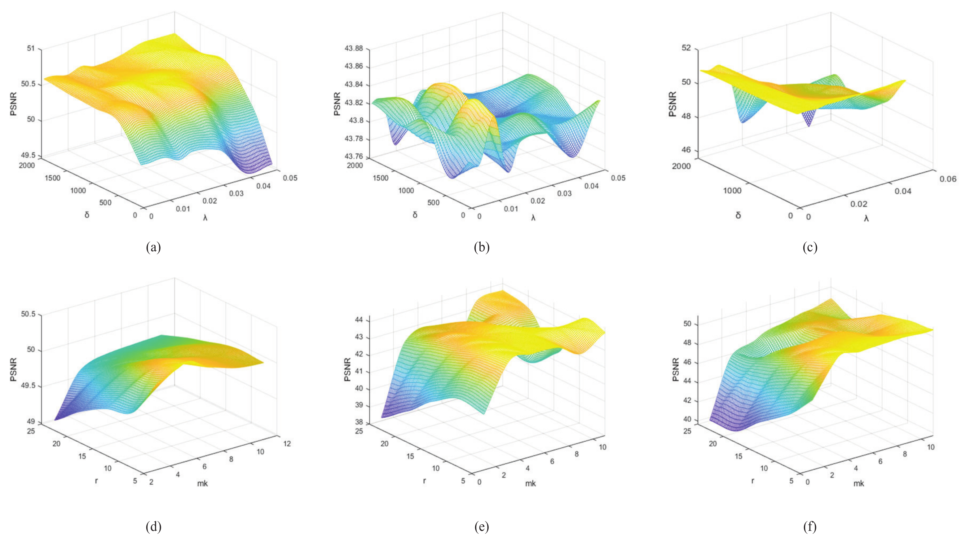
5.1. Parameters Selection

There are five important parameters for our proposed method, including δ , λ , τ , m k and r. δ weighs the relationship between the two fidelity terms. λ and τ are penalty factors for the two regular terms. m k determines the number of each cluster, and r determines the size of the tensor dictionary.
Figure 11a–c show the psnr values as a function of parameter δ and parameter λ on the simulated three data sets, respectively. For these experiments, δ was selected from [100 500 1000 1500 2000] and λ was chosen from [0.001 0.005 0.01 0.015 0.02 0.03 0.04 0.05]. It can be seen from Figure 11a–c that the values of parameters δ and λ do have a great influence on the experimental results. However, for the three data sets, when parameter δ   =   10 3 , the local optimal values of parameter λ may be reached. Therefore, we set λ   =   0.03 for PU, λ   =   0.01 for WDC, λ   =   0.01 for HOS, respectively. In addition, Figure 12a shows the psnr as a function of parameter τ on the WDC dataset. It could be seen that the proposed SSTSR exhibited stable performance when τ   = 10,000. Furthermore, we also found that setting τ   = 10,000 was also robust for both PU and HOS datasets.
Besides, we also discussed the number of nonlocal clusters m k and the number of dictionary atoms r. First, we set the range of [1 3 5 7 9 11] for m k . The selection of r should not only consider the reduction of the subspace dimension, but also ensure that enough spectral information was retained. The range of r was set to [5 10 15 20 25]. As can be seen in Figure 11d–f, the PSNR of the reconstructed images of the three datasets reached the maximum value when r   =   5 . Because of the difference of similar spatial information in each dataset, the values of m k for the three datasets were slightly different, so we set m k   =   5 for PU, m k = 5 for WDC, m k   =   9 for HOS, respectively. In addition, for the non-local clustering algorithm used in our method, the size of the nonlocal clustering patch was set to 20   ×   20 and the step size was set to 8.

5.2. Convergence Behavior

Taking University of Pavia and Washington DC Mall as examples, Figure 12b shows the relative error calculated by X ( i + 1 ) X ( i ) F / X ( i ) F of the reconstructed image as a function of iterations. It is clear that the relative error decreases sharply in the initial stage, and then continues to decrease in a relatively smooth trend until the relative error is close to 0. This verifies that our proposed SSTST method has strong convergence. When the number of iterations is 15, the tolerance threshold of the algorithm can be reached.

5.3. Effectiveness of the Spectral Smooth Prior and Tubal Sparsity Constraint

In this subsection, we discuss the influence of each regular term on the reconstructed results. First, we did the related experiments on data set 2. From Table 3, we can find that the ERGAS index with only the spectral smoothing constraint is lower than the ERGAS index without the spectral smoothing constraint, and the lower the ERGAS index, the better the fusion quality of the spectrum, which fully invalidates the effeciveness of the spectral smoothing constraint. By adding tube row-sparseness constraint on the basis, the PSNR increases by 0.3 dB, which validates that the constraints imposed on both dictionaries and coefficients are reasonable and effective.

6. Conclusions

In this article, we propose a SSTSR model for HSI super-resolution, which employs the tensor sparse representation framework based on t-product. The proposed SSTSR method puts forward continuity constraints on tensor dictionary to improve the spectral smoothness of HSI, and introduces tubal row-sparse constraints on tensor coefficients to exploit their inherent sparse structure. It fully considers the relationship between nonlocal modes and tensor decomposition factors. Besides, ADMM algorithm is used to efficiently solve our model. Extensive experimental results show that the SSTSR method can significantly improve the spatial resolution of LR-HSI while preserving the spectral curves.
In the near future, we will improve the performance of our method in three aspects. First, because the spectral reflectance of ground objects is non-negative, limiting the non-negativity of the dictionary has practical physical significance for hyperspectral image super-resolution. Second, our method relies on the estimation of the spectral subspace of the reconstructed nonlocal clustering tensor, and we subsequently consider speeding up the algorithm by adaptively choosing the subspace spectral dictionary size. Furthermore, we will refer to more efficient hyperparameter optimization methods to reduce the computational cost.

Author Contributions

Conceptualization, Funding acquisition, Methodology, Supervision, Validation, L.S.; Investigation, Software, Visualization, Writing–original draft, Q.C.; Major revision, L.S. and Z.C.; Experiment comparison, Response comments, Z.C. All authors have read and agreed to the published version of the manuscript.

Funding

This research was funded in part by the National Natural Science Foundation of China [61971233, 62076137], the Henan Key Laboratory of Food Safety Data Intelligence [KF2020Z-D01].

Institutional Review Board Statement

Not applicable.

Informed Consent Statement

Not applicable.

Data Availability Statement

All datasets used in this study can be found at the following link. The “University of Pavia” dataset is linked to http://www.ehu.eus/ccwintco/index.php/Hyperspectral_Remote_Sensing_Scenes. The “Washington DC Mall” dataset is linked to https://engineering.purdue.edu/~biehl/MultiSpec/hyperspectral.html. The “Houston” dataset is linked to http://www.grss-ieee.org/community/technical-committees/data-fusion, all link accessed on 29 January 2022.

Conflicts of Interest

The authors declare no conflict of interest.

References

  1. Sun, L.; He, C. Hyperspectral Image Mixed Denoising Using Difference Continuity-Regularized Nonlocal Tensor Subspace Low-Rank Learning. IEEE Geosci. Remote Sens. Lett. 2022, 19, 1–5. [Google Scholar] [CrossRef]
  2. Drumetz, L.; Meyer, T.R.; Chanussot, J.; Bertozzi, A.L.; Jutten, C. Hyperspectral Image Unmixing With Endmember Bundles and Group Sparsity Inducing Mixed Norms. IEEE Trans. Image Process. 2019, 28, 3435–3450. [Google Scholar] [CrossRef] [PubMed]
  3. Sun, L.; Zhao, G.; Zheng, Y.; Wu, Z. Spectral-Spatial Feature Tokenization Transformer for Hyperspectral Image Classification. IEEE Trans. Geosci. Remote Sens. 2022, 60, 1–14. [Google Scholar] [CrossRef]
  4. He, N.; Paoletti, M.E.; Haut, J.M.; Fang, L.; Li, S.; Plaza, A.; Plaza, J. Feature Extraction with Multiscale Covariance Maps for Hyperspectral Image Classification. IEEE Trans. Geosci. Remote Sens. 2019, 57, 755–769. [Google Scholar] [CrossRef]
  5. Song, X.; Zou, L.; Wu, L. Detection of Subpixel Targets on Hyperspectral Remote Sensing Imagery Based on Background Endmember Extraction. IEEE Trans. Geosci. Remote Sens. 2021, 59, 2365–2377. [Google Scholar] [CrossRef]
  6. Xu, Q.; Li, B.; Zhang, Y.; Ding, L. High-Fidelity Component Substitution Pansharpening by the Fitting of Substitution Data. IEEE Trans. Geosci. Remote Sens. 2014, 52, 7380–7392. [Google Scholar] [CrossRef]
  7. Jiao, J.; Wu, L. Image Restoration for the MRA-Based Pansharpening Method. IEEE Access 2020, 8, 13694–13709. [Google Scholar] [CrossRef]
  8. Leung, Y.; Liu, J.; Zhang, J. An Improved Adaptive Intensity–Hue–Saturation Method for the Fusion of Remote Sensing Images. IEEE Geosci. Remote Sens. Lett. 2014, 11, 985–989. [Google Scholar] [CrossRef]
  9. Duran, J.; Buades, A. Restoration of Pansharpened Images by Conditional Filtering in the PCA Domain. IEEE Geosci. Remote Sens. Lett. 2019, 16, 442–446. [Google Scholar] [CrossRef] [Green Version]
  10. Restaino, R.; Dalla Mura, M.; Vivone, G.; Chanussot, J. Context-Adaptive Pansharpening Based on Image Segmentation. IEEE Trans. Geosci. Remote Sens. 2017, 55, 753–766. [Google Scholar] [CrossRef] [Green Version]
  11. Restaino, R.; Vivone, G.; Addesso, P.; Chanussot, J. A Pansharpening Approach Based on Multiple Linear Regression Estimation of Injection Coefficients. IEEE Geosci. Remote Sens. Lett. 2020, 17, 102–106. [Google Scholar] [CrossRef]
  12. Vivone, G.; Marano, S.; Chanussot, J. Pansharpening: Context-Based Generalized Laplacian Pyramids by Robust Regression. IEEE Trans. Geosci. Remote Sens. 2020, 58, 6152–6167. [Google Scholar] [CrossRef]
  13. Dong, W.; Liang, J.; S, X. Saliency Analysis and Gaussian Mixture Model-Based Detail Extraction Algorithm for Hyperspectral Pansharpening. IEEE Trans. Geosci. Remote Sens. 2020, 58, 5462–5476. [Google Scholar] [CrossRef]
  14. Zheng, Y.; Li, J.; Li, Y.; Guo, J.; Wu, X.; Chanussot, J. Hyperspectral Pansharpening Using Deep Prior and Dual Attention Residual Network. IEEE Trans. Geosci. Remote Sens. 2020, 58, 8059–8076. [Google Scholar] [CrossRef]
  15. Huck, A.; Guillaume, M.; Blanc-Talon, J. Minimum Dispersion Constrained Nonnegative Matrix Factorization to Unmix Hyperspectral Data. IEEE Trans. Geosci. Remote Sens. 2010, 48, 2590–2602. [Google Scholar] [CrossRef]
  16. Yokoya, N.; Yairi, T.; Iwasaki, A. Coupled Nonnegative Matrix Factorization Unmixing for Hyperspectral and Multispectral Data Fusion. IEEE Trans. Geosci. Remote Sens. 2012, 50, 528–537. [Google Scholar] [CrossRef]
  17. Simões, M.; Bioucas-Dias, J.; Almeida, L.; Chanussot, J. A Convex Formulation for Hyperspectral Image Superresolution via Subspace-Based Regularization. IEEE Trans. Geosci. Remote Sens. 2015, 53, 3373–3388. [Google Scholar] [CrossRef] [Green Version]
  18. Zhang, K.; Wang, M.; Yang, S. Multispectral and Hyperspectral Image Fusion Based on Group Spectral Embedding and Low-Rank Factorization. IEEE Trans. Geosci. Remote Sens. 2017, 55, 1363–1371. [Google Scholar] [CrossRef]
  19. Akhtar, N.; Shafait, F.; Mian, A. Bayesian sparse representation for hyperspectral image super resolution. In Proceedings of the 2015 IEEE Conference on Computer Vision and Pattern Recognition (CVPR), Boston, MA, USA, 7–12 June 2015; pp. 3631–3640. [Google Scholar] [CrossRef]
  20. Dong, W.; Fu, F.; Shi, G.; Cao, X.; Wu, J.; Li, G.; Li, X. Hyperspectral Image Super-Resolution via Non-Negative Structured Sparse Representation. IEEE Trans. Image Process. 2016, 25, 2337–2352. [Google Scholar] [CrossRef]
  21. Han, X.; Wang, J.; Shi, B.; Zheng, Y.; Chen, Y. Hyper-spectral Image Super-resolution Using Non-negative Spectral Representation with Data-Guided Sparsity. In Proceedings of the 2017 IEEE International Symposium on Multimedia (ISM), 11–13 December 2017; pp. 500–506. [Google Scholar] [CrossRef]
  22. Han, X.; Yu, J.; Xue, J.H.; Sun, W. Hyperspectral and Multispectral Image Fusion Using Optimized Twin Dictionaries. IEEE Trans. Image Process. 2020, 29, 4709–4720. [Google Scholar] [CrossRef]
  23. Han, X.; Shi, B.; Zheng, Y. Self-Similarity Constrained Sparse Representation for Hyperspectral Image Super-Resolution. IEEE Trans. Image Process. 2018, 27, 5625–5637. [Google Scholar] [CrossRef] [PubMed]
  24. Wei, Q.; Bioucas-Dias, J.; Dobigeon, N.; Tourneret, J. Hyperspectral and Multispectral Image Fusion Based on a Sparse Representation. IEEE Trans. Geosci. Remote Sens. 2015, 53, 3658–3668. [Google Scholar] [CrossRef] [Green Version]
  25. Ye, Q.; Huang, P.; Zhang, Z.; Zheng, Y.; Fu, L.; Yang, W. Multiview Learning With Robust Double-Sided Twin SVM. IEEE Trans. Cybern. 2021, 1–14. [Google Scholar] [CrossRef] [PubMed]
  26. Xue, J.; Zhao, Y.Q.; Bu, Y.; Liao, W.; Chan, J.C.W.; Philips, W. Spatial-Spectral Structured Sparse Low-Rank Representation for Hyperspectral Image Super-Resolution. IEEE Trans. Image Process. 2021, 30, 3084–3097. [Google Scholar] [CrossRef]
  27. Sun, L.; Wu, F.; He, C.; Zhan, T.; Liu, W.; Zhang, D. Weighted Collaborative Sparse and L1/2 Low-Rank Regularizations With Superpixel Segmentation for Hyperspectral Unmixing. IEEE Geosci. Remote Sens. Lett. 2022, 19, 1–5. [Google Scholar] [CrossRef]
  28. Dong, C.; Loy, C.; He, K.; Tang, X. Image Super-Resolution Using Deep Convolutional Networks. IEEE Trans. Pattern Anal. Mach. Intell. 2016, 38, 295–307. [Google Scholar] [CrossRef] [Green Version]
  29. Palsson, F.; Sveinsson, J.; Ulfarsson, M. Multispectral and Hyperspectral Image Fusion Using a 3-D-Convolutional Neural Network. IEEE Geosci. Remote Sens. Lett. 2017, 14, 639–643. [Google Scholar] [CrossRef] [Green Version]
  30. Zhang, X.; Huang, W.; Wang, Q.; Li, X. SSR-NET: Spatial–Spectral Reconstruction Network for Hyperspectral and Multispectral Image Fusion. IEEE Trans. Geosci. Remote Sens. 2021, 59, 5953–5965. [Google Scholar] [CrossRef]
  31. Yang, J.; Zhao, Y.; Chan, J.W. Hyperspectral and Multispectral Image Fusion via Deep Two-branches Convolutional Neural Network. Remote Sens. 2018, 10, 800. [Google Scholar] [CrossRef] [Green Version]
  32. Wei, W.; Nie, J.; Li, Y.; Zhang, L.; Zhang, Y. Deep Recursive Network for Hyperspectral Image Super-Resolution. IEEE Trans. Comput. Imaging 2020, 6, 1233–1244. [Google Scholar] [CrossRef]
  33. Wang, Z.; Chen, B.; Lu, R.; Zhang, H.; Liu, H.; Varshney, P.K. FusionNet: An Unsupervised Convolutional Variational Network for Hyperspectral and Multispectral Image Fusion. IEEE Trans. Image Process. 2020, 29, 7565–7577. [Google Scholar] [CrossRef]
  34. Hu, J.; Tang, Y.; Fan, S. Hyperspectral Image Super Resolution Based on Multiscale Feature Fusion and Aggregation Network With 3-D Convolution. IEEE J. Sel. Top. Appl. Earth Obs. Remote Sens. 2020, 13, 5180–5193. [Google Scholar] [CrossRef]
  35. Zheng, K.; Gao, L.; Liao, W.; Hong, D.; Zhang, B.; Cui, X.; Chanussot, J. Coupled Convolutional Neural Network With Adaptive Response Function Learning for Unsupervised Hyperspectral Super Resolution. IEEE Trans. Geosci. Remote Sens. 2021, 59, 2487–2502. [Google Scholar] [CrossRef]
  36. He, C.; Sun, L.; Huang, W.; Zhang, J.; Jeon, B. TSLRLN: Tensor Subspace Low-Rank Learning with Non-local Prior for Hyperspectral Image Mixed Denoising. Signal Process. 2021, 184, 108060. [Google Scholar] [CrossRef]
  37. Li, S.; Dian, R.; Fang, L.; Bioucas-Dias, J. Fusing Hyperspectral and Multispectral Images via Coupled Sparse Tensor Factorization. IEEE Trans. Image Process. 2018, 27, 4118–4130. [Google Scholar] [CrossRef] [PubMed]
  38. Dian, R.; Li, S.; Fang, L.; Lu, T.; Bioucas-Dias, J. Nonlocal Sparse Tensor Factorization for Semiblind Hyperspectral and Multispectral Image Fusion. IEEE Trans. Cybern. 2020, 50, 4469–4480. [Google Scholar] [CrossRef]
  39. Wan, W.; Guo, W.; Huang, H.; Liu, J. Nonnegative and Nonlocal Sparse Tensor Factorization-Based Hyperspectral Image Super-Resolution. IEEE Trans. Geosci. Remote Sens. 2020, 58, 8384–8394. [Google Scholar] [CrossRef]
  40. Kanatsoulis, C.I.; Fu, X.; Sidiropoulos, N.D.; Ma, W.K. Hyperspectral Super-Resolution: A Coupled Tensor Factorization Approach. IEEE Trans. Signal Process. 2018, 66, 6503–6517. [Google Scholar] [CrossRef] [Green Version]
  41. Dian, R.; Li, S.; Fang, L. Learning a Low Tensor-Train Rank Representation for Hyperspectral Image Super-Resolution. IEEE Trans. Neural Netw. Learn. Syst. 2019, 30, 2672–2683. [Google Scholar] [CrossRef]
  42. Dian, R.; Li, S. Hyperspectral Image Super-Resolution via Subspace-Based Low Tensor Multi-Rank Regularization. IEEE Trans. Image Process. 2019, 28, 5135–5146. [Google Scholar] [CrossRef]
  43. Xu, H.; Qin, M.; Chen, S.; Zheng, Y.; Zheng, J. Hyperspectral-Multispectral Image Fusion via Tensor Ring and Subspace Decompositions. IEEE J. Sel. Top. Appl. Earth Obs. Remote Sens. 2021, 14, 8823–8837. [Google Scholar] [CrossRef]
  44. Kilmer, M.E.; Martin, C.D. Factorization Strategies for Third-order Tensors. Linear Algebra Its Appl. 2011, 435, 641–658. [Google Scholar] [CrossRef] [Green Version]
  45. Xu, Y.; Wu, Z.; Chanussot, J.; Wei, Z. Nonlocal Patch Tensor Sparse Representation for Hyperspectral Image Super-Resolution. IEEE Trans. Image Process. 2019, 28, 3034–3047. [Google Scholar] [CrossRef] [PubMed]
  46. Zhang, Z.; Aeron, S. Denoising and Completion of 3D Data via Multidimensional Dictionary Learning. arXiv 2015, arXiv.1512.09227. [Google Scholar] [CrossRef]
  47. Boyd, S.; Parikh, N.; Chu, E.; Peleato, B.; Eckstein, J. Distributed Optimization and Statistical Learning via the Alternating Direction Method of Multipliers. Found. Trends® Mach. Learn. 2011, 3, 1–122. [Google Scholar] [CrossRef]
  48. Kilmer, M.E.; Braman, K.; Hao, N.; Hoover, R.C. Third-order Tensors as Operators on Matrices: A Theoretical and Computational Framework with applications in imaging. SIAM J. Matrix Anal. Appl. 2013, 34, 148–172. [Google Scholar] [CrossRef] [Green Version]
  49. Ram, I.; Elad, M.; I, C. Image Processing Using Smooth Ordering of its Patches. IEEE Trans. Image Process. 2013, 22, 2764–2774. [Google Scholar] [CrossRef] [Green Version]
  50. Ye, Q.; Yang, J.; Liu, F.; Zhao, C.; Ye, N.; Yin, T. L1-Norm Distance Linear Discriminant Analysis based on an Effective Iterative Algorithm. IEEE Trans. Circuits Syst. Video Technol. 2018, 28, 114–129. [Google Scholar] [CrossRef]
  51. Ye, Q.; Zhao, H.; Li, Z.; Yang, X.; Gao, S.; Yin, T.; Ye, N. L1-Norm Distance Minimization-Based Fast Robust Twin Support Vector k -Plane Clustering. IEEE Trans. Neural Netw. Learn. Syst. 2018, 29, 4494–4503. [Google Scholar] [CrossRef]
  52. Liu, L.; Peng, G.; Wang, P.; Zhou, S.; Wei, Q.; Yin, S.; Wei, S. Energy-and Area-efficient Recursive-conjugate-gradient-based MMSE detector for Massive MIMO Systems. IEEE Trans. Signal Process. 2020, 68, 573–588. [Google Scholar] [CrossRef]
  53. Yokoya, N.; Grohnfeldt, C.; Chanussot, J. Hyperspectral and Multispectral Data Fusion: A comparative review of the recent literature. IEEE Geosci. Remote Sens. Mag. 2017, 5, 29–56. [Google Scholar] [CrossRef]
  54. Xu, S.; Amira, O.; Liu, J.; Zhang, C.X.; Zhang, J.; Li, G. HAM-MFN: Hyperspectral and Multispectral Image Multiscale Fusion Network With RAP Loss. IEEE Trans. Geosci. Remote Sens. 2020, 58, 4618–4628. [Google Scholar] [CrossRef]
  55. Dian, R.; Li, S.; Kang, X. Regularizing Hyperspectral and Multispectral Image Fusion by CNN Denoiser. IEEE Trans. Neural Netw. Learn. Syst. 2021, 32, 1124–1135. [Google Scholar] [CrossRef] [PubMed]
Figure 1. A tensor signal represented by a tensor-linear combination of i tensor dictionary atoms.
Remotesensing 14 02142 g001
Figure 2. Flowchart of SSTSR method.
Remotesensing 14 02142 g002
Figure 3. Spectral smoothing regularization term and restoration results of the spectrum at location (2,2). (a) Fidelity term with tensor decomposition X k = D k A k . (b) Image obtained by spectral difference operator. (c) Spectral smoothing regularization term on the sub-tensor D k . (d) spectral curve with spectral-smoothness constraint. (e) spectral curve without spectral-smoothness constraint.
Remotesensing 14 02142 g003
Figure 4. Tubal row-sparse constraints for coefficient tensor, the red tubes in the coefficient tensors stand for the non-zero tubes, and green ones are zero tubes. The image on the far right is the visualization matrix of A k expanded along the second dimension.
Remotesensing 14 02142 g004
Figure 5. The first and third rows show the false color images (composited by bands 70, 35, 5) of the comparison methods on the University of Pavia data set. The second and fourth rows show the normalized residual images of the comparison methods at band-50.
Remotesensing 14 02142 g005
Figure 6. The first and third rows show the false color images (composited by bands 65, 45, 5) of the comparison methods on the Washington DC Mall data set. The second and fourth rows show the normalized residual images of the comparison methods at band-50.
Remotesensing 14 02142 g006
Figure 7. The first and third rows show the false color images (composited by bands 70, 45, 5) of the comparison methods on the Houston data set. The second and fourth rows show the normalized residual images of the comparison methods at band-50.
Remotesensing 14 02142 g007
Figure 8. Spectral curve comparison and spectral curve residual comparison for three data sets.
Remotesensing 14 02142 g008
Figure 9. PSNR values against different spectral bands on three data sets.
Remotesensing 14 02142 g009
Figure 10. Super-resolution results of all comparison methods at band 90 on real data set.
Remotesensing 14 02142 g010
Figure 11. The first row shows the psnr as a function of parameter λ and parameter δ on three data sets. The second row shows the psnr as a function of parameter m k and parameter r on three data sets. (a,d) University of Pavia. (b,e) Washington DC Mall. (c,f) Houston.
Remotesensing 14 02142 g011
Figure 12. (a) PSNR as a function of parameter τ for Washington DC Mall. (b) Relative error of the reconstructed image for successive iterations for PU and WDC.
Remotesensing 14 02142 g012
Publisher’s Note: MDPI stays neutral with regard to jurisdictional claims in published maps and institutional affiliations.

