Article

Using Satellite-Based Data to Facilitate Consistent Monitoring of the Marine Environment around Ireland

1
National Centre for Geocomputation, Maynooth University, Maynooth, Co. Kildare, Ireland
2
Faculdade Ciências e Tecnologia, Universidade do Algarve, 8005-139 Faro, Portugal
3
CEAUL—Centro de Estatística e Aplicações, Faculdade de Ciências, Universidade de Lisboa, 1749-016 Lisboa, Portugal
*
Author to whom correspondence should be addressed.
Remote Sens. 2022, 14(7), 1749; https://doi.org/10.3390/rs14071749
Submission received: 26 February 2022 / Revised: 27 March 2022 / Accepted: 29 March 2022 / Published: 6 April 2022
(This article belongs to the Special Issue Remote Sensing for Shallow and Deep Waters Mapping and Monitoring)

Abstract

:
As an island nation, Ireland needs to ensure effective management measures to protect marine ecosystems and their services, such as the provision of fishery resources. The characterization of marine waters using satellite data can contribute to a better understanding of variations in the upper ocean and, consequently, the effect of their changes on species populations. In this study, nineteen years (1998–2016) of monthly data of essential climate variables (ECVs), chlorophyll (Chl-a), and the diffuse attenuation coefficient (K490) were used, together with previous analyses of sea surface temperature (SST), to investigate the temporal and spatial variability of surface waters around Ireland. The study area was restricted to specific geographically delineated divisions, as defined by the International Council of the Exploration of the Seas (ICES). The results showed that SST and Chl-a were positively and significantly correlated in ICES divisions corresponding to oceanic waters, while in coastal divisions, SST and Chl-a showed a significant negative correlation. Chl-a and K490 were positively correlated in all cases, suggesting an important role of phytoplankton in light attenuation. Chl-a and K490 had significant trends in most of the divisions, reaching maximum values of 1.45% and 0.08% per year, respectively. The strongest seasonal Chl-a trends were observed in divisions VIId and VIIe (the English Channel), primarily in the summer months, followed by northern divisions VIa (west of Scotland) and VIb (Rockall) in the winter months.

1. Introduction

The potential of the world’s oceans to provide food and nutrition for the growing global population is widely recognised [1], and it is expected to reach 9.7 billion people by 2050 (FAO, 2016). The seas around Ireland are considered one of the most productive and biologically sensitive areas in European Union (EU) waters. As an island nation, fishery resources are highly important to the economy and society. In 2020, Irish vessels landed a total of 188,994 tonnes of fish catch in Irish ports, with an estimated value of EUR 220.5 million [2], and with another EUR 31.5 million landed abroad [3]. According to the Irish Seafood Development Agency, Bord Iascaigh Mhara (BIM), 16,430 people were employed directly and downstream in the Irish seafood sector in 2020.
The value and importance of fishery resources make their responsible management essential. Despite remarkable progress in some areas, the overall downward trend in global marine fish stocks has not improved [1]. Previous attempts to manage either single- or multi-species fish stocks without considering their population dynamics and without accounting for environmental variability have systematically failed, sometimes with catastrophic ecological and economic consequences, such as global declines in fish populations [4] and the collapse of fisheries [5]. Widespread recognition of these shortcomings has led to the development of a set of principles, guidelines, and strategies, known as the Ecosystem Approach to Fisheries Management (EAFM) [6,7]. This approach explicitly recognises that fisheries are entities dependent on biological dynamics, which are strongly influenced by ecological, social, and economic elements and changes. EAFM aims to improve the understanding of the factors responsible for changes in abundance and spatial distribution of exploited fish stocks, to decouple the impacts of fisheries on the marine environment from natural environmental influences, and ultimately, to implement more effective management systems [8,9].
It is widely recognised that the physical and biological characteristics of pelagic habitats can influence the distribution and abundance of fish populations by affecting prey availability, larval distribution and survival, and migration patterns [10,11]. Over the years, it has been recognised that the key to understanding fish population variability lies in understanding the variables affecting the pelagic ecosystem when fish are in their larval stage [12]. Since the larval stage is generally planktonic, it is mostly a captive of its environment and cannot travel far to seek optimal survival conditions. Several studies address the effects of climate change on marine species and marine ecosystems as a whole [13,14], and directly link temporal and spatial changes in climate variables to fish abundance [15,16]. Global ocean warming increased by 0.13 °C per decade between 1971 and 2010 [17], and this rate is predicted to continue over the next 100 years [18]. The waters of the northeast Atlantic have warmed at a faster rate compared to the global ocean, and the distribution and changes in the relative abundance of various fish species have been observed at local, regional, and global scales [19,20]. Understanding the effects of environmental conditions and their changes on the abundance and distribution of exploited fish stocks is a key challenge for developing management strategies [21], especially under the influence of climate change effects. The use of environmental data (e.g., SST, Chl-a) in analysing, assessing, and predicting fishery health is therefore essential. The assessment of the status and appropriate management of living marine resources depend on a proper understanding of the complex relationship between marine environmental processes and biological dynamics [22].
A major barrier to the operational implementation of EAFM has been the sparse availability of information on the state of the broader marine ecosystem structure and processes [23]. In recent years, efforts to implement EAFM concepts have greatly increased [24,25], partly in response to legislation. However, actual implementation of EAFM strategies remains a challenge, with significant obstacles to overcome [26,27]. Satellite-based data offer great potential for applications in fisheries, including marine resource management, stock assessment, marine aquaculture site selection, detection of harmful algal blooms, or habitat change monitoring [12]. Remote sensing tools can provide a wide range of indicators of ecosystem health over large areas, including an accurate description of the pelagic ecosystem at a given time and location [28]. Advances in remote sensing technology and the efficient use of satellite-based data are proving to be resourceful and an integral component in implementing EAFM strategies at regional and global scales. Recent advances in satellite sensors and technologies under the Copernicus Programme, the EU’s Earth Observation Programme, has facilitated a new era of satellite data and the derivation of a variety of oceanic and atmospheric datasets, with high spatial and temporal resolutions that are freely available to potential users. Despite the current and future prospects for using satellite-based marine data to assess the functioning of marine ecosystems, satellite data remain underutilized by practitioners and policymakers in fishery management.
In this context, the main objective of this work is to strengthen the use of satellite data to provide reliable products for monitoring the marine environment. To this end, we will characterise the temporal and spatial variability of ECVs variables such as Chl-a and the diffuse attenuation coefficient for the downwelling spectral irradiance at 490 nm wavelength (K490), in specific areas around Ireland defined by the International Council for the Exploration of the Seas (ICES), extending previous work on the temporal and spatial variability of seasurface temperature (SST) [29].

2. Materials and Methods
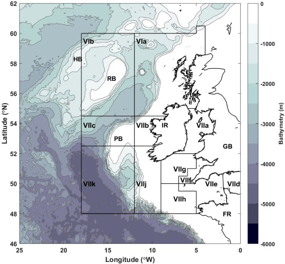
2.1. Study Area

The study area is composed by 12 ICES divisions known as the North Western Waters (NWW) (Figure 1). The study area includes sub-area VI composed of the ICES divisions VIa (west of Scotland) and VIb (Rockall), and sub-area VII formed by ICES divisions VIIa (Irish Sea), VIIb (west of Ireland), VIIc (Porcupine Bank), VIId (eastern English Channel), VIIe (western English Channel), VIIf (Bristol Channel), VIIg (north Celtic Sea), VIIh (south Celtic Sea), VIIj (southwest of Ireland—east), and VIIk (southwest of Ireland—west). The NWW covers approximately 1.15 million km2 and includes the entire exclusive economic zone (EEZ) of Ireland and part of the EEZs of the United Kingdom (UK) and France [30].
NWW waters are very productive, supporting a rich and diverse range of ecosystems, habitats, and species. Some of the most extensive and valuable sea fishery resources in Europe are found off the Irish coast, and the region is considered an ideal location for finfish, shellfish, and seaweed aquaculture [31]. The oceanographic characterisation of these economically important divisions, using satellite data, can contribute to a better understanding of upper ocean environmental changes and, consequently, the effects of these changes on species populations.

2.2. Satellite-Derived Essential Climate Variables (ECVs)

Nineteen years (January 1998–December 2016) of monthly chlorophyll-a (Chl-a) and diffuse attenuation coefficient for the downwelling spectral irradiance at 490 nm (K490) were used to assess the temporal and spatial variability within the surface waters surrounding Ireland. The Chl-a and K490 products were obtained from the Ocean Colour Climate Change Initiative (OC-CCI) dataset, version 3.1, with a spatial resolution of ~4 km/pixel. The OC-CCI dataset is based on ocean colour data, registered by MERIS, MODIS-Aqua and VIIRS, with band shifting, bias correction, and per-pixel uncertainty calculation applied to align the SeaWiFS bands to produce a consistent climate-quality dataset. The biases between sensors from different missions can generate a significant false trend, which could affect findings derived from time-series analysis [32]. Products from OC-CCI have been shown to be more consistent over time, compared to other multi-mission products, than single-mission and other merged ocean colour satellite products [33].
The generation of the OC-CCI v3.1 Chl-a algorithm involved the blending of the Ocean Colour Index (OCI) [34], the OC5 algorithm [35], adopted for coastal regions, and the OC3 [36] and OC4 [37] algorithms. The blended Chl-a algorithm, used in versions v3.0 and v3.1, attempts to weight the outputs of the best-performing algorithms (OC3, OCI (OC4 + CI), and OC5), which are based on the water types present, further improving performance in Case-2 waters compared to earlier versions, which were mainly open-ocean focused [38]. Some filters were applied to the products, considering the realistic values of each parameter. In the case of Chl-a, all the values less than 0.001 were set to 0.001 mg/m3, while the values greater than 100 mg/m3 were set to 100 mg/m3 [34]. The diffusive attenuation coefficient at 490 nm for downwelling irradiance (K490), which is an apparent optical property (AOP), was computed from the inherent optical properties (IOPs) at 490 nm using Lee et al.’s (2005) algorithm. K490 can be considered an indicator of turbidity, directly related to the presence of scattering particles in the water column. It indicates how strongly light is attenuated within the water column at a specific wavelength—in this case, 490 nm. Considering IOPs, all values greater than 10 (1/m) were discarded [34]. More detailed information about the OC-CCI v3.1 dataset can be found in the product user guide [38]. In November 2020, ESA Ocean Colour project released the v5.0 dataset, which incorporates Sentinel-3 A-OLCI data. The new v5.0 OC-CCI product extends the data availability until the end of June 2020, including associated per-pixel uncertainty information. The dataset used in this study does not correspond to the latest v5.0 version. However, this issue does not affect the application of our methodology and the results derived from it, as the main difference between both datasets corresponds to the time spans.
In addition to the Chl-a and K490 OC-CCI products (Figure 2), daily sea surface temperature (SST) data, covering the same nineteen years (January 1998–December 2016), were obtained from the NOAA Reynolds Optimal Interpolation SST (OISST) dataset, version v2.0, with a spatial resolution of 25 km. Selecting this dataset instead of the one produced by OC-CCI corresponds to a practical reason, since SST values had already been extracted and analysed for the same study area [29]. The OISST version v2.0 is a global dataset created using the International Comprehensive Ocean-Atmosphere Data Set (ICOADS) and AVHRR Pathfinder data. In this dataset, the operational AVHRR products were used along with in situ data from ships and buoys to allow for the large-scale adjustment of satellite biases [39]. More detailed information on this dataset can be found in previous studies [39,40,41,42].

2.3. Statistical Analyses

Firstly, an exploratory analysis was performed to summarise the main characteristics of the Chl-a, K490, and SST data in the study area. Subsequently, spatial and temporal variability analyses were performed with respect to the 19 years of monthly Chl-a and K490 data. Trend analyses were also performed for both parameters, complementing previous temporal and spatial SST analyses [29].

2.3.1. Time Series Decomposition

A time series can be defined as a collection of observations on a variable of interest. Most time-series analyses, based on remote sensing data, use the classical decomposition X = S + T + I, where S, T, and I represent the seasonal, trend, and irregular (or residual) components, respectively [43]. However, this approach does not allow for a flexible specification of the seasonal component, while the trend component is represented by a deterministic function of time that is easily affected by outlying observations. In this study, the time series were decomposed using the stl.fit () procedure [44,45], built on the Seasonal-Trend decomposition based on Loess (STL, local polynomial regression fitting) [46], where Loess is a nonlinear estimating method [46]. One of the advantages of the “stl.fit ()” function is its capability to identify a seasonal component that changes over time, responds to nonlinear trends, and is robust to outliers. This is achieved by smoothing the time series, using Loess, in two loops: an inner loop, which iterates between the seasonal and trend smoothing; and the outer loop, which minimises the effect of outliers, locating them in the irregular, or residual component [46]. The irregular/residual component is derived by subtracting the seasonal and trend time series components [46]. STL, as other non-parametric regression methods, requires the subjective selection of seasonal and trend smoothing parameters [46]. The Loess smoothing parameters, applicable to the STL analysis, must be defined in advance and set according to the user’s knowledge of the data [47,48]. The STL algorithm [44], applied in this study, allows a selective choice of the STL smoothing parameters and selects the best STL model based on the lowest error (in our case, the root mean squared error). This fact is beneficial for studies of time series that need to evaluate interannual variability. We direct the reader to previous studies for more information on the STL approach [44,45,46].

2.3.2. Non-Parametric Trend Analysis

Once the seasonal component was extracted, Sen’s slope was calculated using the Mann–Kendall test [49,50]. The Mann–Kendall test is used to statistically evaluate a monotonic upward or downward trend of the variable of interest over time. A monotonic upward (downward) trend means that the variable is consistently increasing (decreasing) over time; however, the trend may or may not be linear [49,50]. The Mann–Kendall test does not require a normal distribution of the residuals resulting from the fitted regression line [49,50]. Sen’s slope is a nonparametric estimator that uses a median value to estimate the slope and is quite robust in the presence of outliers.
Additionally, to identify cases where structural changes (i.e., points where the changes are more pronounced) might occur, we used the statistical R package “strucchange” [51] and its “breakpoints ()” function. The “breakpoints ()” function allows to identify breakpoints that minimise the residual sum of squares of a linear model with m + 1 segments. The optimal number of structural breaks is determined using the Bayesian information criterion (BIC) [51]. This analysis allowed the identification of significant changes (e.g., trend shifts) in the time series of each ICES division.
Monthly trends and significance levels were also calculated, using the “wql” R package [52] and the “seasonTrend ()” function, which calculates the signs and magnitudes of trends for individual months [53]. “SeasonTrend ()” is based on the Mann–Kendall test and calculates the actual and relative Sen´s slope, the p-values for the trend, and the fraction of missing slopes encompassing the first and last fifths of the data [53]. This analysis can be informative because some time series may not show a significant trend overall but may show a significant trend for individual months, such that the direction of the trend varies from month to month.

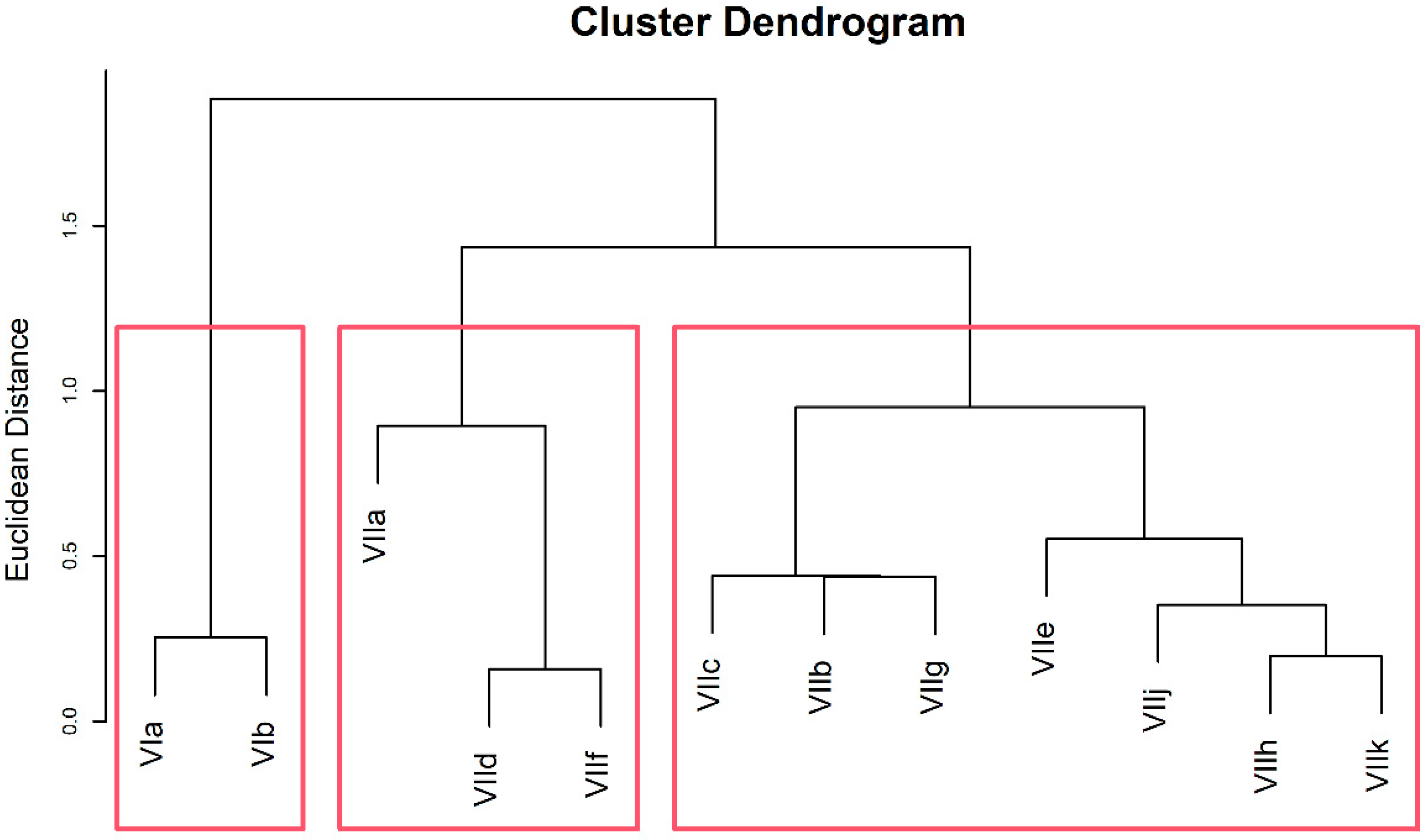
2.3.3. Similarities between ICES Divisions

To examine similarities among divisions with respect to Chl-a, K490, and SST, an agglomerative hierarchical cluster analysis using the climatology values for each ICES division was performed. In hierarchical cluster analysis, data are grouped into homogeneous clusters by merging data points, or classes, one at a time in a series of sequential steps [54,55]. Here, we use agglomerative hierarchical cluster analysis, also known as bottom-up clustering. In the initial stage of the algorithm, each n data point is considered as a single cluster [56]. Then, in each step, the two most similar data points or clusters are combined into a larger cluster, resulting in n − 1 clusters [56]. Similarities or proximities are determined by a distance function, in our case the Euclidean distance, which corresponds to the squared distance between data points or vectors. For details on agglomerative hierarchical algorithms, we refer the reader to previous overviews [57].

3. Results

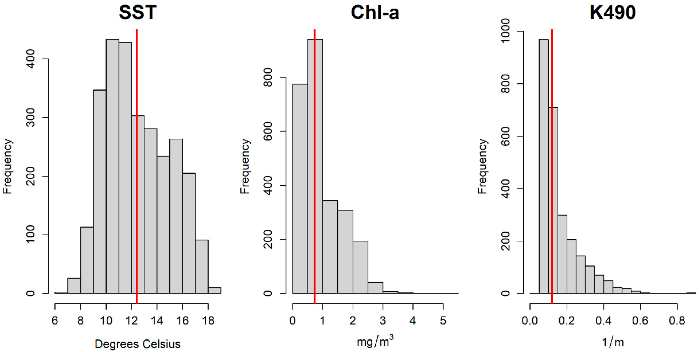
3.1. Exploratory Statistical Analyses

Exploratory analysis, including all ICES divisions (Figure 3), showed a median SST of 12.04 °C, with the most common values between 9 °C and 12 °C (Figure 3). The data distribution considerably changed in the case of Chl-a and K490. Both variables showed a highly skewed distribution to the right with a median value of 0.74 mg/m3 for Chl-a and 0.12 1/m for K490. The most common values for Chl-a in the time series were lower than 1 mg/m3, while for K490, the most common values were lower than 0.1 1/m, indicating a general first optical depth (Z90 = 1/K490) of 10 m. This value (Z90) represents the layer depth from which 90% of the water leaves radiance that the satellite register comes from.
The three ECVs—Chl-a, K490, and SST—showed a significant correlation in almost all divisions (Table 1). SST and Chl-a showed significant correlation in all divisions except for division VIIj (southwest of Ireland—east). In most cases, there is an inverse relationship between SST and Chl-a. Significant and positive SST-Chl-a correlations were found within oceanic divisions, such as divisions VIa (west of Scotland) and VIb (Rockall), as well as in ICES divisions located on the west coast of Ireland such as divisions VIIc (Porcupine Bank) and VIIk (south of Ireland—west) (Table 1). The highest SST-Chl-a correlations were negative and found in divisions VIIa (Irish Sea), VIIg (north Celtic Sea), and VIIf (Bristol Channel), all of them highly influenced by coastal processes and dynamics (e.g., tidal mixing, stratification intensity, freshwater input/river runoff). Overall, SST and K490 showed a significant positive correlation in most of the divisions, except for divisions located in more oceanic waters, where the relationship was primarily negative. Chl-a and K490 showed significant and positive relations in all ICES divisions, suggesting that the attenuation of light in the first meters of the water column could mainly depend on phytoplankton biomass.

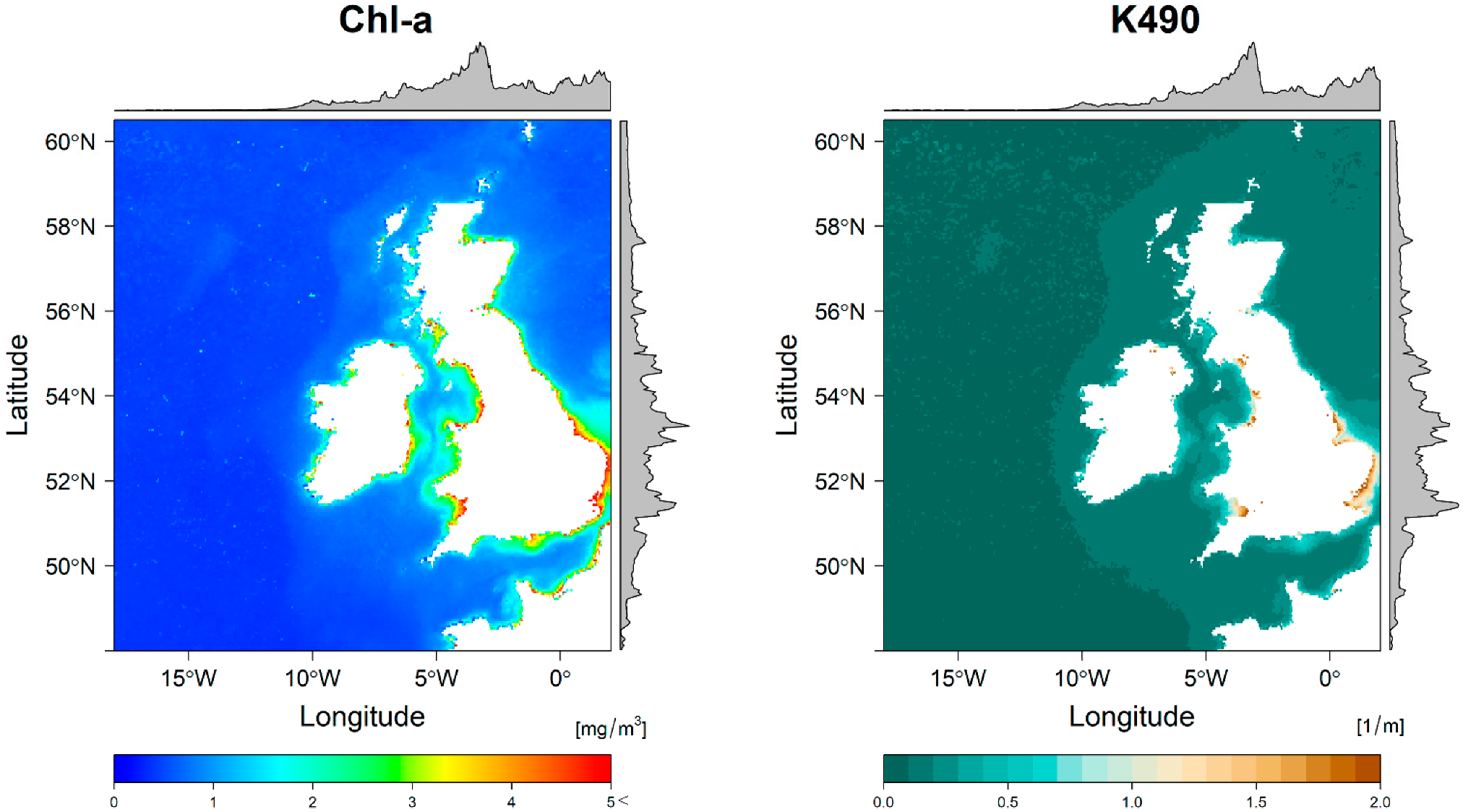
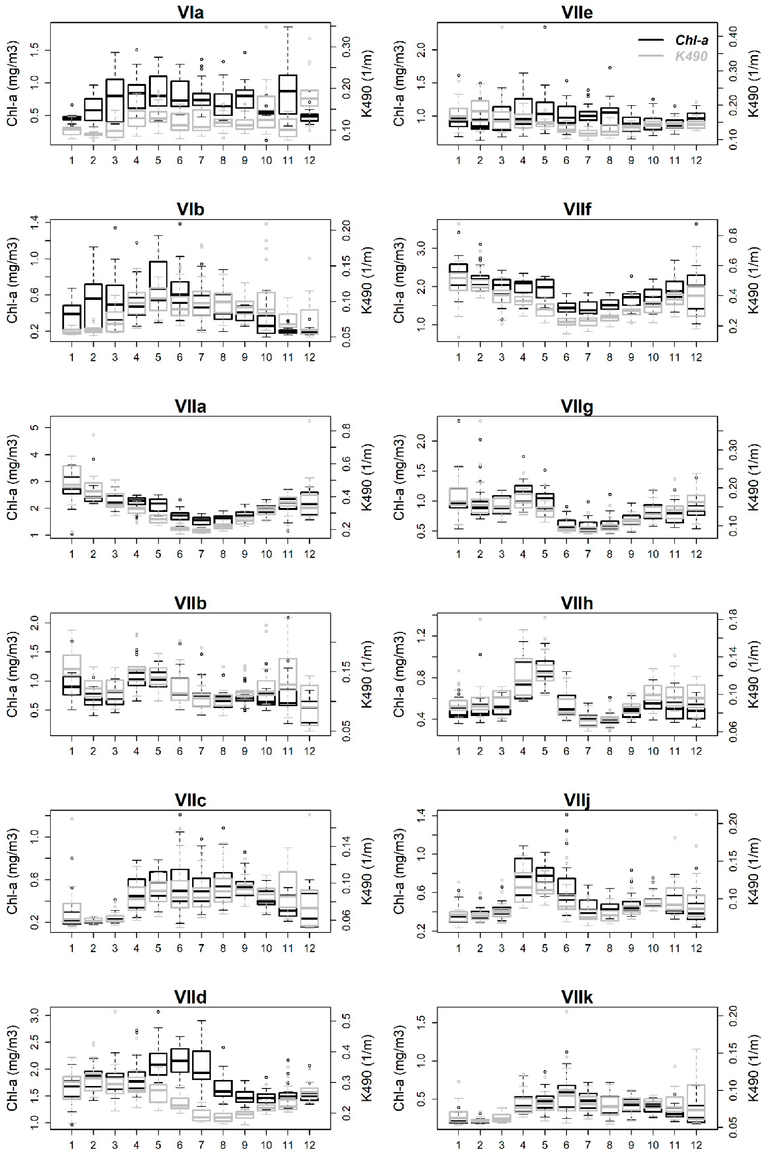
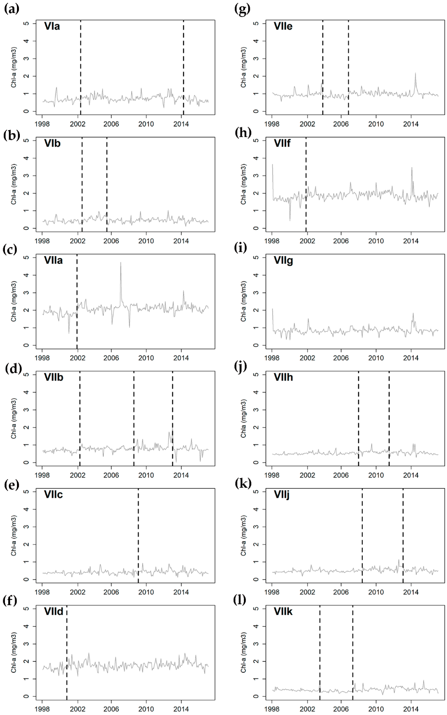
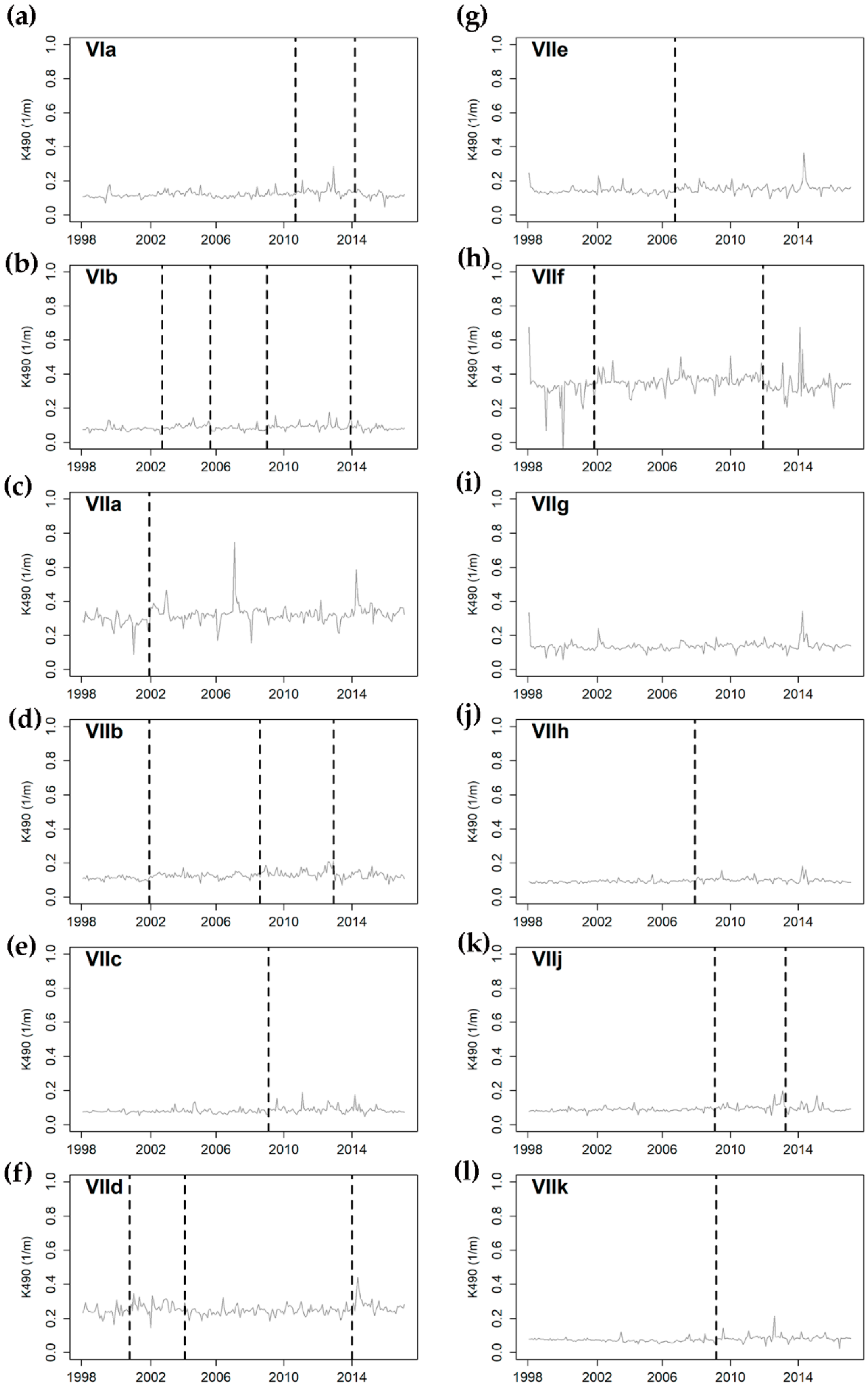
3.2. Chl-a and K490 Temporal and Spatial Variability

The Chl-a distribution, in the nineteen-year monthly climatology, showed a clear seasonal variation that was spatially dependent (Figure 4). The ICES divisions that showed the highest Chl-a concentrations (median ± standard deviation) corresponded to VIIa (2.00 ± 0.51 mg/m3), VIIf (1.81 ± 0.43 mg/m3), and VIId (1.73 ± 0.35 mg/m3), while the lowest Chl-a concentrations were found on VIIk (0.36 ± 0.22 mg/m3), VIIc (0.39 ± 0.28 mg/m3), and VIb (0.42 ± 0.39 mg/m3). Considering annual values, the highest Chl-a values (median ± standard deviation) were found in 2009 (0.87 ± 0.84 mg/m3), 2011 (0.87 ± 0.95 mg/m3), and 2012 (0.86 ± 0.86 mg/m3), while the lowest values were found in 2016 (0.60 ± 0.91 mg/m3), 1998 (0.60 ± 0.88 mg/m3), and 2001 (0.63 ± 0.73 mg/m3). The highest monthly Chl-a values were found in May (0.96 ± 0.43 mg/m3), while the lowest Chl-a values were found in February (0.59 ± 0.48 mg/m3).
The nineteen-year monthly climatology of K490 showed consistency with the Chl-a spatial distribution, indicating a well-delimited differentiation between coastal and more open waters (Figure 4). The spatial distribution of K490 showed the highest values (>1 1/m) in areas near the coast, mostly in the bays. Considering the different ICES divisions, the highest values were found in VIIf (0.33 ± 0.11 1/m), VIIa (0.29 ± 0.11 1/m) and VIId (0.24 ± 0.15 1/m), while the lowest values were in VIIk (0.07 ± 0.015 1/m), VIIc (0.08 ± 0.023 1/m), and VIb (0.08 ± 0.03 1/m). The annual values (median ± standard deviation) were the highest in 2009 (0.14 ± 0.10 1/m), 2012 (0.13 ± 0.10 1/m), and 2014 (0.13 ± 0.12 1/m), while 2016 (0.11 ± 0.12 1/m), 1998, and 2001 (0.10 ± 0.10 1/m) showed the lowest values. The highest K490 monthly values were detected in wintertime—December (0.16 ± 0.11 1/m) and January (0.15 ± 0.10 1/m)—whereas the lowest K490 values were observed in the summertime—July and August (0.10 ± 0.04 1/m). The finding of the highest K490 values in the winter months is not surprising since, for example, higher amounts of terrestrial runoff increase the amount of resuspended material and tidal-driven turbidity within coastal/nearshore areas. However, K490 values in winter should be treated with caution, as cloud cover and light conditions may affect absolute values due to data gaps.

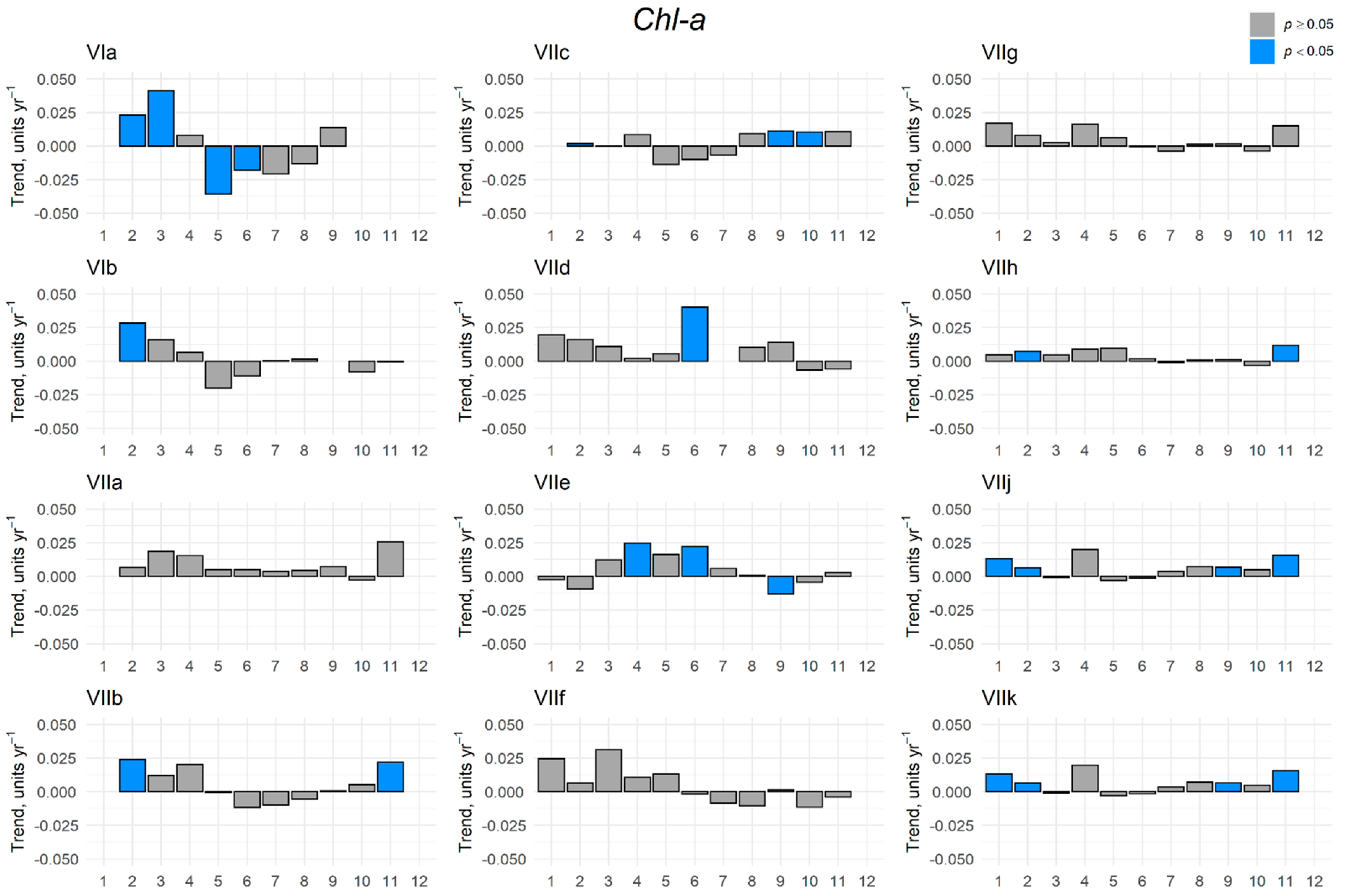
3.3. Chl-a Temporal Trends

Nineteen years of monthly data (January 1998–December 2016) were used to determine temporal trends of Chl-a in each of the ICES divisions. Most of the ICES divisions showed a significant (p-value ≤ 0.05) and positive trend, indicating an increase in Chl-a concentration (Table 2). The strongest trends were observed in ICES divisions located in the southeastern part of the study area, VIIa (Irish Sea) and VIId (eastern English Channel), with a Sen’s Slope (SS) of 0.014 mg/m3/year and 0.010 mg/m3/year, respectively. The lowest values were found in ICES divisions located in the most western areas such as VIIc (Porcupine Bank) with a trend of 0.004 mg/m3/year followed by the ICES divisions VIIk (southwest of Ireland—west) and VIIh (south Celtic Sea) with a trend of 0.005 mg/m3/year in both cases. ICES divisions located in the northern areas, VIa (west of Scotland) and VIb (Rockhall), did not show any significant Chl-a trend.
Most of the ICES divisions showed at least one structural change in Chl-a concentration (Figure 5), except division VIIg (north Celtic Sea), which did not present any. The largest number of breakpoints was found in VIIb (west of Ireland), indicating a high variability in this area.
The signs and magnitudes of trends for individual months were also computed because they may behave differently from the general computed trend (Figure 6). The monthly analysis can provide a more comprehensive idea of how Chl-a values behave between seasons. The ICES divisions VIIa (Irish Sea), VIIf (Bristol Channel), and VIIg (north Celtic Sea), all of them located close to each other, did not show any significant trend between seasons. The ICES divisions VIIb (west of Ireland) and VIIh (south Celtic Sea) showed the same pattern with positive trends in the winter months. Similar behaviour was found in VIIj (southwest of Ireland—east) and VIIk (southwest of Ireland—west), but these ICES divisions also showed a significant and positive trend in late summer (September). The ICES divisions located in northern areas, VIa (west of Scotland) and VIb (Rockall), showed increasing Chl-a values in winter months. However, VIa (west of Scotland) showed a significant negative trend in late spring–early summer. The ICES divisions corresponding to the English Channel showed different behaviour between them. VIId (western English Channel), most influenced by surrounding coastal areas, showed a significant and positive trend in summer months, whereas VIIe (eastern English Channel) showed positive trends in spring and summer months but negative trends in autumn (September).
The magnitude of Chl-a trends was different between ICES divisions. The strongest trends were found in ICES divisions VIId and VIIe (the English Channel), mainly in summer months, followed by the northern ICES divisions VIa (west of Scotland) and VIb (Rockhall) in winter months. High increments in Chl-a trend values were also found in the west of Ireland (VIIb) in the summer months.

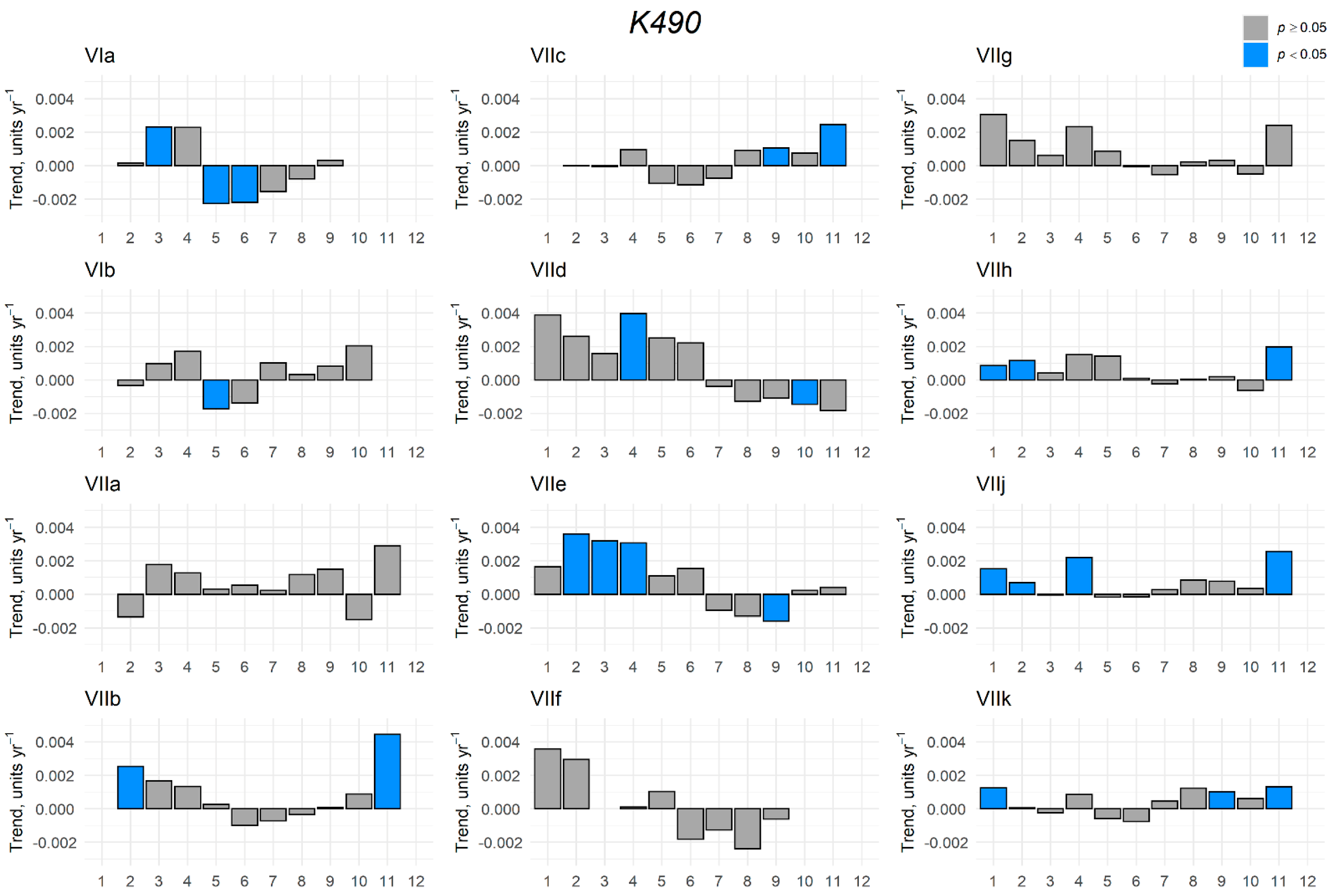
3.4. K490 Temporal Trends

As in the case of Chl-a, 19 years of monthly data (January 1998–December 2016) were used to extract the temporal trends of K490 in each of the ICES divisions. A significant K490 trend was detected in almost all divisions, except for VIIa (Irish Sea), VIId (eastern English Channel), and VIIf (Bristol Channel). Due to the nature of the data (very low values), the percentage per year was used for comparison (Table 3). The highest trends were found in division VIIe (eastern English Channel) with 0.125% per year, followed by VIIg (north Celtic Sea) and VIIj (south of Ireland—east) with 0.078% per year, respectively (Table 3). The lowest significant trends in K490 values were found in divisions VIIh (south Celtic Sea) with a trend of 0.040% per year and VIIc (Porcupine Bank) and VIIb (Rockall) with a value of 0.042% per year. All significant trends were positive, indicating an increment of K490 values and, consequently, a decrease in the attenuation depth and water quality.
The monthly K490 time series were also analysed to detect unusual shifts in K490 values (Figure 7). Only in division VIIg (north Celtic Sea) was no shift in K490 values detected, as was the case for Chl-a, indicating temporal stability in this area. The behaviour of K490 in the remaining ICES divisions was quite variable, but one or two breakpoints were observed in most of them. Breakpoints in K490 trends were found in coastal divisions, such as VIIa (Irish Sea), VIIf (Bristol Channel), and VIId (eastern English Channel). The breakpoints occurred at different times, suggesting that they could be caused by local conditions. Most of the K490 breakpoints were coincident with the ones obtained for Chl-a values. However, new breakpoints were found for in VIIf (Bristol Channel) and VIId (eastern English Channel). These results suggest that factors other than phytoplankton concentration influence the water attenuation and turbidity. Light penetration is strongly attenuated by particulate and dissolved matter originating from river runoff, or which could be re-suspended from the seabed due to strong vertical tidal mixing [58]. The Bristol Channel and its adjacent coastal seas, for example, are considered to be one of the most energetic European continental shelf areas, exhibiting some of the largest spring tides and tide ranges, which contribute to sediment resuspension [59].
Analysis of monthly trends for K490 showed variability among ICES divisions (Figure 8). As with the Chl-a time series analysis, there were no significant trends for K490 in some ICES divisions. These divisions were VIIa (Irish Sea), VIIf (Bristol Channel), and VIIg (north Celtic Sea). ICES divisions located in the southwest of Ireland such as VIIb (west of Ireland), VIIc (Porcupine), VIIh (south Celtic Sea), VIIj (southwest of Ireland—east), and VIIk (southwest of Ireland—west) showed positive and significant trends (p-value ≤ 0.05) in winter months, with some slight differences between them. Moreover, ICES divisions located in oceanic waters such as VIa (west of Scotland) and VIb (Rockall) showed negative and significant trends in summer months. In the case of VIa (west of Scotland), it showed negative trends in summer and positive trends in spring and autumn. This could indicate a possible reduction in the summer phytoplankton bloom in this area and a shift to the spring and autumn months, as Chl-a and K490 parameters are strongly correlated in this ICES division (r = 0.86, p-value ≤ 0.001). A significant and positive trend was observed in spring in the case of VIId and VIIe, both corresponding to the English Channel, while a negative and significant trend was observed in autumn. In the case of VIIe (eastern English Channel), the results were coincident with the trends of Chl-a. The strongest trends were found in spring in the English Channel and west of Ireland.

4. Discussion

Chl-a, K490, and SST parameters can provide a comprehensive picture of the biophysical properties of both oceanic and coastal surface waters, e.g., [11,60,61]. Chl-a and SST are considered ECVs, which, together with turbidity, are used by the Marine Strategy Framework Directive (MSDF) for assessing the Good Environmental Status (GES). In addition, SST, Chl-a, and K490 are among the marine biophysical parameters strongly influencing the distribution of pelagic fish, e.g., due to their effects on, for example, recruitment, survival conditions, distribution, migration patterns, feeding rate, or spawning, e.g., [60,61,62,63,64,65,66,67,68].
As previously mentioned, pelagic fisheries such as mackerel, herring, and blue whiting are among Ireland´s most important seafood resources. Ireland’s 2020 environmental assessment, conducted by the Environmental Protection Agency (EPA), reported that the status of commercial fish and shellfish stocks was not fully compatible with Good Environmental Status [69]. The Irish Fisheries Ecosystems Advisory Services (FEAS) found that the number of sustainably fished stocks has slightly decreased, and 13 stocks remained overfished in 2020 [70]. On the other hand, fisheries are one of the economic sectors that will be most affected by Brexit. More than 70% of the total Irish fishing fleet over 12 m in length, which operate in both whitefish and pelagic fisheries, would be affected by the loss of access to UK waters [71]. Therefore, understanding species distribution is key to optimizing fishing efforts and the sustainability of these resources in the future.
Satellite imagery has been used as a tool to support fish population studies and their changes, e.g., [7,11,72]. This study showed that SST was significantly and negatively related to Chl-a in most of the ICES divisions, indicating a decrease in Chl-a concentration with an increase in SST. This relationship was more pronounced in divisions located close to the coast, such as divisions VIIa (Irish Sea), VIIf (Bristol Channel), and VIId (eastern English Channel). The most likely cause of this relationship could be an increase in the stratification and a deepening of the thermocline leading to a reduction in nutrients in the euphotic zone [73]. Significant and positive correlations between SST and Chl-a were detected in oceanic divisions, such as VIa (west of Scotland) and VIb (Rockall), and in divisions located off the west coast of Ireland, such as VIIc (Porcupine Bank) and VIIk (southwest of Ireland—west). The significant positive correlations between SST and Chl-a could be explained by the temporal cycles of phytoplankton, which strongly depend on seasonal changes in the vertical water column structure, e.g., [74,75]. Seasonal solar stratification plays a crucial role in determining the light and nutrient requirements for phytoplankton growth and the onset of blooms throughout the year, e.g., [74]. As the spring season progresses, solar heating generates a buoyance flux that stabilizes the water column and, together with increased solar radiation, triggers the spring phytoplankton bloom in waters around Ireland, e.g., [72,74]. However, prolonged stratification would impair nutrient regeneration and thus negatively affect primary production. Significant increases in SST have been observed in some areas around Ireland [29], with trends ranging from 0.28 °C to 0.20 °C per decade [29]. If this warming trend continues in the future, it could lead to persistent stratification of the water column, resulting in a decrease in Chl-a concentration and, consequently, affecting local phytoplankton abundance and the food web that depends on it.
The results presented in this study also showed that surface waters around Ireland exhibit high spatial variability in Chl-a and K490 values. The highest Chl-a and K490 values were found in coastal divisions, such as divisions VIIa (Irish Sea), VIIf (Bristol Channel), and VIId (eastern English Channel). These results were consistent with in situ oceanographic data obtained through scientific surveys, e.g., the PELTIC12 survey [76]. Coastal areas are highly influenced by terrestrial runoff and associated inputs of nutrients, such as nitrogen and phosphorus, which can lead to increases in phytoplankton biomass. High Chl-a levels often indicate poor water quality, and the long-term persistence of these high values is considered an indicator of an environmental problem such as eutrophication [77]. Other studies, e.g., [78], have also found an increase in Chl-a levels in the northeast Atlantic between 52° N and 58° N since the mid-1980s. Our study suggests that this trend is continuing, and that Chl-a values are increasing in these areas.
Seasonal variability of Chl-a in Irish waters shows a high peak in spring and a low peak in autumn [75]. In winter, low light conditions inhibit phytoplankton growth, but in spring (March to April), phytoplankton biomass increases in response to increasing solar irradiance levels [75]. After the spring bloom, Chl-a levels decrease due to a combination of factors, including zooplankton grazing, nutrient depletion, and sedimentation [75]. An autumn bloom, which is shorter and less intense than a spring bloom, usually marks the end of the autumn seasonal growing period [75]. In our analysis, this pattern was evident in divisions VIIg and VIIh (the Celtic Sea), VIIb, (west of Ireland), and VIIj (southwest of Ireland—east). However, other patterns were also detected. Several ICES divisions were characterised by a single and prolonged peak in Chl-a values with its maximum detected in spring and summer months. The areas that showed this behaviour mainly corresponded to ICES divisions located in the west of Ireland, such as the divisions VIb (Rockall), VIIc (Porcupine Bank), and VIIk (southwest of Ireland—west). This single and long-lasting peak could be explained by a succession of different phytoplankton groups, such as the abundance of diatoms in spring and autumn and the dominance of dinoflagellates in summer [75]. Other authors have described the same behaviour in Chl-a values in the eastern Atlantic Ocean (a single peak in summer months), caused by above-average concentrations of particulate inorganic carbon (PIC) [79]. In coastal ICES divisions, such as divisions VIIa (the Irish Sea) and VIId (Bristol Channel), Chl-a did not show any particular patterns, except for minimum Chl-a values detected during the summer months. These coastal divisions often receive a considerable amount of terrestrial and riverine runoff, most notably in winter months, resulting in nutrient enrichment. Other studies reported different behaviour of Chl-a values in these areas. For example, some authors [80] reported an increase in Chl-a concentrations in the spring in the Irish Sea, which corresponds to division VIIa in this study. These authors reported that Chl-a levels in the Irish Sea reach a peak between March and May, or June, with concentrations higher than 40 mg/m3 [80]. In this study, we did not find such high concentrations, probably because we used monthly averages rather than isolated in situ measurements, or due to recent and continuous changes in environmental conditions.
Both Chl-a and K490 showed significant increasing trends in most ICES divisions. This result differs from our preliminary analyses [81], which found no trends in Chl-a values, using the same time series of data. This fact highlights the importance of considering the presence of outliers when calculating temporal trends of oceanographic variables such as Chl-a. To decompose the Chl-a and K490 time series and extract the temporal trends, the Seasonal and Trend decomposition using Loess (STL), incorporated in the R software function “stl.fit ()” [44], was used. The STL method has been shown to be robust to extreme values and unusual observations, i.e., outliers, and avoids effects on seasonal and trend components without reducing the size of the dataset [44]. The significant trends reported in this study were based on a nineteen-year, monthly time series. However, some studies have reported that a minimum length of the Chl-a time series is required to obtain a reliable trend value. For example, Beaulieu et al. [33] considered that continuous Chl-a time series of at least 27 years are required, while Henson et al. [82] estimated the minimum period to be 39 years. Beaulieu et al. [33] also stated that a minimum period of 43 years is required if the time series is interrupted. In any case, satellite data time series are constantly growing, and new missions will continue to maintain the temporal continuity of these data in the future, offering an unprecedented source of information for trend analysis.
One of the most important ecological insights from multidecadal observations is that changes can occur abruptly as discrete shifts from one state to another [53]. These changes can reveal important information about trends that cannot be detected with simple trend analysis [83]. In our case, most of the ICES divisions exhibited some structural change during these 19 years, with the exception of division VIIg (north Celtic Sea). This fact could be explained by the oceanographic nature of the Celtic Sea, which is surrounded by several fronts, such as the Irish Sea Front to the north, and the Ushant Front to the east. These fronts, along with the continental shelf in the southern part and some eddies produced by tidal currents, may provide some stability to this area. Even these assumptions should be studied in more detail, it is known that oceanographic fronts can separate water masses that may change little over hundreds of kilometres.
The highest number of structural changes was detected in division VIIb (west of Ireland). This high variability could be explained by the influence of freshwater input and nutrients from the Shannon, Clare (Corrib), and Laune rivers. In some ICES divisions, which include oceanic or intermediate depth waters, Chl-a exhibited multiple structural changes that coincided in time. In general, most Chl-a breakpoints within oceanic divisions were found in wintertime, between October and December. However, it is quite difficult to determine the causes of these shifts due to the lack of comprehensive monitoring programmes that would allow in-depth investigation of specific processes. For example, the observed structural Chl-a change between October and December 2002 spans over divisions VIa (west of Scotland), VIb (Rockall), VIIa (Irish Sea), VIIb (west of Ireland), and VIIf (Bristol Channel), indicating a relatively large-scale process. The mixing of upper ocean waters is strongly stimulated by the passage of weather systems during winter and early spring, disrupting the development of water-column stratification, bringing up nutrients, and thus influencing the timing of the seasonal increase in phytoplankton [84]. The variability and intensity of such mixing events are associated with atmospheric synoptic events, or storms [84], which would directly affect the variability and intensity of phytoplankton blooms. A chain of low-pressure systems (a persistent large low-pressure system) have been recorded in October 2002 [85]. The passage of these low-pressure systems could have initiated and promoted phytoplankton blooms over an extensive area, resulting in the observed October–December 2002 Chl-a breakpoints. The breakpoints in both the K490 and Chl-a time series were coincident in time, suggesting, as previously discussed, a direct relationship between both parameters and dependence between water attenuation and Chl-a values.
As expected, the analyses presented here have shown that Chl-a and K490 exhibit similar cycles and patterns in different ICES divisions, generally within divisions that are spatially close to each other. Marine waters are a fluid and ever-changing environment that do not fit strictly within the boundaries of the ICES-defined divisions and sub-areas, primarily outlined as geo-political delaminations. Considering Chl-a, K490, and SST parameters, a hierarchical cluster analysis revealed that the divisions considered could be categorised into three main groups (Figure 9). Two of the main groups could be classified as oceanic (VIa and VIb) and coastal (VIIa, VIIf, and VIId) waters, while the largest number of divisions could be designated as intermediate waters (VIIb, VIIc, VIIe, VIIg, VIIh, VIIj, and VIIk). This fact suggests that considering each division as an isolated and discrete management area could lead to a mismatch between environmental processes and associated fish population behaviour.
The transition from single-species fishery management to an ecosystem approach continues to progress, as environmental factors are incorporated into fish stock assessments, resulting in more appropriate and more effective management tools and systems, e.g., [7]. EAFM implementation requires a high temporal frequency of sampling, often over large regions. This study demonstrates that satellite data can provide a cost-effective and time-efficient approach to qualitatively and quantitatively assessing biophysical conditions and changes in the marine surface waters. SST trends are already influencing the onset of spawning, migration, and distribution of blue whiting, northeast Atlantic mackerel, and western horse mackerel as well as the recruitment of some gadoids in the Irish Sea, Celtic Sea, and west of Scotland [86]. The recently reported SST increase in surface waters around Ireland over the period 1982–2015 [29] and the changes in Chl-a trends reported in this study may already have implications for the life cycles and dynamics of fish populations. Pelagic fish species, such as herring, blue whiting, northeast Atlantic mackerel, and horse mackerel, are keystones of the food web, and changes in their abundance can have significant impacts throughout the marine food chain.
A systematic monitoring of biophysical changes and trends in the marine environments will be key to understanding the complex dynamics of marine ecosystems, especially bottom-up (primary production) forcing. Satellite-based data, in conjunction with conventional ship-based data, will enable the development and use of informative and reliable marine ecosystem indicators and variables (e.g., SST, Chl-a, turbidity) and support continuous assessment of the biotic and abiotic components of the marine ecosystem. Despite the recognised interactions between marine species and their environment, spatial management approaches remain largely limited to static boundaries and isolated sampling stations [87]. Consequently, any introduced fixed-time area closures would not always encompass the core habitat of species of concern and could unjustifiably restrict (or allow) fishing activity [87]. Static or seasonal area closures are usually based on historical data on species distribution, thus putting these areas at risk of losing ecological relevance as species’ distributions shift with changing climate and human activity [87]. Satellite data could add value to species distribution models, where the major focus is to identify spatial patterns in datasets [88]. In addition, satellite-based data could be useful in developing ecological response models to better understand the responses of species to changes in environmental variables [89,90].

5. Conclusions

In recent years, legislation and policy sectors have emphasised the need for a holistic approach to decision making for the protection and management of marine areas and living resources. The primary goal of EAFM is to maintain the health of marine ecosystems while ensuring appropriate use of marine resources for the benefit of present and future generations. A major limitation in the practical implementation of EAFM for fishery management is the sparse availability of information on the status of the overall ecosystem structure and processes. To overcome this limitation, some countries have made significant investments to support and maintain routine monitoring of the marine environment and fish populations.
In this context, satellite-based information can help fill existing data gaps and facilitate surface water assessment and monitoring. No other observational strategy can provide synoptic views of upper ocean optical properties with such a high spatial and temporal resolution and extent. This study demonstrates the advantages and benefits of satellite-based data in providing up-to-date knowledge of the ecosystem status of Irish waters, confided within ICES-defined divisions. The study also contribute to promote the incorporation of satellite-based data into living marine resource management, such as fishery management.

Author Contributions

Conceptualization, G.C. and C.C.; methodology, G.C. and C.C.; formal analysis, G.C.; investigation, G.C. and C.C.; resources, G.C. and C.C.; writing—original draft preparation, G.C.; writing—review and editing, G.C., C.C. and T.M.; funding acquisition, G.C. and T.M. All authors have read and agreed to the published version of the manuscript.

Funding

G.C. and T.M. were supported by the European Union’s Horizon 2020 research and innovation programme under grant agreement No 869710, corresponding to the project Marine Coastal Ecosystems Biodiversity and Services in a Changing World (MaCoBioS). C.C. was partially financed by national funds through FCT—Fundação para a Ciência e a Tecnologia under the project UIDB/00006/2020. GC received the Marine Institute Networking and Travel grant NT/18/22 to visit the University of Algarve.

Data Availability Statement

The data used in this study are openly available via http://www.oceancolour.org (accessed on 31 January 2022). The data can be directly downloaded from ftp://oc-cci-data:ELaiWai8ae@oceancolour.org (accessed on 31 January 2022).

Acknowledgments

The authors acknowledge the Ocean Colour Climate Change Initiative and the European Space Agency for the OC-CCI dataset. We are thankful to Angelina Smilenova for her comments and suggestions, and the design of Figure 1.

Conflicts of Interest

The authors declare no conflict of interest. The funders had no role in the design of the study; in the collection, analyses, or interpretation of data; in the writing of the manuscript, or in the decision to publish the results.

References

  1. FAO. The State of World Fisheries and Aquaculture 2016. Contributing to Food Security and Nutrition for All; Food and Agriculture Organization of the United Nations: Rome, Italy, 2016. [Google Scholar]
  2. ICES. The Stock Book 2020: Annual Review of Fish Stocks in 2020 with Management Advice for 2021; Marine Institute: Galway, Ireland, 2020. [Google Scholar]
  3. ICES. The Stock Book. Report to the Minister for Agriculture, Food, and the Marine. Annual Review of Fish Stocks in 2021 with Management Advice for 2022; Marine Institute: Galway, Ireland, 2021. [Google Scholar]
  4. Juan-Jordá, M.J.; Mosqueira, I.; Cooper, A.B.; Freire, J.; Dulvy, N.K. Global population trajectories of tunas and their relatives. Proc. Natl. Acad. Sci. USA 2011, 108, 20650–20655. [Google Scholar] [CrossRef] [PubMed] [Green Version]
  5. Dickey-Collas, M.; Nash, R.D.M.; Brunel, T.; van Damme, C.J.G.; Marshall, C.T.; Payne, M.R.; Corten, A.; Geffen, A.J.; Peck, M.A.; Hatfield, E.M.C.; et al. Lessons learned from stock collapse and recovery of North Sea herring: A review. ICES J. Mar. Sci. 2010, 67, 1875–1879. [Google Scholar] [CrossRef] [Green Version]
  6. Morishita, J. What is the ecosystem approach for fisheries management? Mar. Policy 2008, 32, 19–26. [Google Scholar] [CrossRef]
  7. Chassot, E.; Bonhommeau, S.; Reygondeau, G.; Nieto, K.; Polovina, J.J.; Huret, M.; Dulvy, N.K.; Demarcq, H. Satellite remote sensing for an ecosystem approach to fisheries management. ICES J. Mar. Sci. 2011, 68, 651–666. [Google Scholar] [CrossRef] [Green Version]
  8. Garcia, S.M.; Zerbi, A.; Chi, D.T.; Lasserre, G. The Ecosystem Approach to Fisheries. Issues, Terminology, Principles, Institutional Foundations, Implementation and Outlook; FAO Fisheries Technical Paper: Rome, Italy, 2003; p. 443. [Google Scholar]
  9. Cury, P.; Shin, Y.-J.; Planque, B.; Durant, J.-M.; Fromentin, J.-M.; Kramer-Schadt, S.; Stenseth, N.C.; Travers, M.; Grimm, V. Ecosystem oceanography for global change in fisheries. Trends Ecol. Evol. 2008, 23, 338–346. [Google Scholar] [CrossRef]
  10. Juan-Jordá, M.J.; Barth, J.A.; Clarke, M.E.; Wakefield, W.W. Groundfish species associations with distinct oceanographic habitats in the Northern California Current. Fish. Oceanogr. 2009, 18, 1–19. [Google Scholar] [CrossRef]
  11. Falcini, F.; Palatella, L.; Cuttitta, A.; Buongiorno-Nardelli, B.; Lacorata, G.; Lanotte, A.S.; Patti, B.; Santoreli, R. The role of hydrodynamic processes on anchovy eggs and larvae distribution in the Sicily Channel (Mediterranean Sea): A case study for the 2004 data set. PLoS ONE 2015, 10, e0123213. [Google Scholar] [CrossRef]
  12. Stuart, V.; Platt, T.; Sathyendranath, S. The future of fisheries science in management: A remote-sensing perspective. ICES J. Mar. Sci. 2011, 68, 644–650. [Google Scholar] [CrossRef] [Green Version]
  13. Boyce, D.G.; Lewis, M.R.; Worm, B. Global phytoplankton decline over the past century. Nature 2010, 466, 591–596. [Google Scholar] [CrossRef]
  14. Mills, K.E.; Pershing, A.J.; Brown, C.J.; Chen, Y.; Chiang, F.S.; Holland, D.S.; Lehuta, S.; Nye, J.A.; Sun, J.C.; Thomas, A.C.; et al. Fisheries management in a changing climate: Lessons from the 2012 ocean heat wave in the Northwest Atlantic. Oceanography 2013, 26, 191–195. [Google Scholar] [CrossRef] [Green Version]
  15. Bellido, J.M.; Pierce, G.J.; Wang, P.J. Modelling intra-annual variation in abundance of squid Loligo forbesi in Scottish waters using generalised additive models. Fish. Res. 2001, 52, 23–39. [Google Scholar] [CrossRef]
  16. Cheung, W.W.L.; Oyinlola, M.A. Vulnerability of flatfish and their fisheries to climate change. J. Sea Res. 2018, 140, 1–10. [Google Scholar] [CrossRef]
  17. Hoegh-Guldberg, O.; Cai, R.; Poloczanska, E.; Brewer, P.; Sundby, S.; Hilmi, K. The Ocean Climate Change 2014: Impacts, Adaptation, and Vulnerability Part B: Regional Aspects Contribution of Working Group II to the Fifth Assessment Report of the Intergovernmental Panel on Climate Change; Barros, V., Field, C., Dokken, D., Mastrandrea, M., Mach, K., Bilir, T., Eds.; Cambridge University Press: Cambridge, NY, USA, 2014; pp. 1655–1731. [Google Scholar]
  18. Phillipart, C.J.M.; Anadón, R.; Donavaro, R.; Dippner, J.W.; Drinkwater, K.F.; Hawkins, S.J.; Oguz, T.; O’Sullivan, G.; Reid, P.C. Impacts of climate change on European marine ecosystems. J. Exp. Mar. Biol. Ecol. 2011, 400, 52–69. [Google Scholar] [CrossRef]
  19. Nye, J.A.; Link, J.S.; Hare, J.A.; Overholtz, W.J. Changing spatial distribution of fish stocks in relation to climate and population size on the Northeast United States continental shelf. Mar. Ecol. Prog. Ser. 2009, 393, 111–129. [Google Scholar] [CrossRef] [Green Version]
  20. Simpson, S.D.; Jennings, S.; Johnson, M.P.; Blanchard, J.L.; Schön, P.J.; Sims, D.W.; Genner, M. Continental shelf-wide response of a fish assemblage to rapid warming of the sea. Curr. Biol. 2011, 21, 1565–1570. [Google Scholar] [CrossRef]
  21. Hofmann, E.E.; Powell, T.M. Environmental variability effects on marine fisheries: Four case studies. Ecol. Appl. 1998, 8, S23–S32. [Google Scholar] [CrossRef] [Green Version]
  22. Makris, N.C.; Ratilal, P.; Jagannathan, S.; Gong, Z.; Andrews, M.; Bertsatos, I.; Godo, O.R.; Nero, R.W.; Jech, J.M. Critical population density triggers rapid formation of vast oceanic fish shoals. Science 2009, 323, 1734–1737. [Google Scholar] [CrossRef] [Green Version]
  23. IOCCG. Remote Sensing in Fisheries and Aquaculture; Forget, M.H., Stuart, V., Platt, T., Eds.; Reports of the International Ocean-Colour Coordinating Group 8: Dartmouth, NS, Canada, 2009. [Google Scholar]
  24. Borja, A.; Elliott, M.; Andersen, J.H.; Berg, T.; Carstensen, J.; Halpern, B.S.; Heiskanen, A.S.; Korpinen, S.; Lowndes, J.S.S.; Martin, G.; et al. Overview of integrative assessment of marine systems: The ecosystem approach in practice. Front. Mar. Sci. 2016, 3, 1–20. [Google Scholar] [CrossRef] [Green Version]
  25. Trochta, J.T.; Pons, M.; Rudd, M.B.; Dirgbaum, M.; Tanz, A.; Hilborn, R. Ecosystem-based fisheries management: Perception on definitions, implementations and aspirations. PLoS ONE 2018, 13, e0190467. [Google Scholar] [CrossRef]
  26. Borja, A.; Galparsoro, I.; Irigoien, X.; Iriondo, A.; Menchaca, I.; Muxika, I.; Pascual, M.; Quincoces, I.; Revilla, M.; Germán Rodríguez, J.; et al. Implementation of the European Marine Strategy Framework Directive: A methodological approach for assessment of environmental status, from the Basque Country (Bay of Biscay). Mar. Pollut. Bull. 2011, 62, 889–904. [Google Scholar] [CrossRef]
  27. Juan-Jordá, M.J.; Murua, H.; Arrizabalaga, H.; Dulvy, N.K.; Restrepo, V. Report card on ecosystem-based fisheries management in tuna regional fisheries management organisations. Fish Fish. 2018, 19, 321–339. [Google Scholar] [CrossRef]
  28. Platt, T.; Sathyhendranath, S. Ecological indicators for the pelagic zone of the ocean from remote sensing. Remote Sens. Environ. 2008, 112, 3426–3436. [Google Scholar] [CrossRef]
  29. Casal, G.; Lavender, S. Spatio-temporal variability of sea surface temperature (SST) in Irish waters (1982–2015) using AVHRR sensor. J. Sea Res. 2017, 129, 89–104. [Google Scholar] [CrossRef]
  30. Dransfeld, L.; Maxwell, H.W.; Moriarty, M.; Nolan, C.; Kelly, E.; Pedreschi, D.; Slattery, N.; Connolly, P. North Western Waters Atlas, 3rd ed.; Marine Institute: Galway, Ireland, 2014. [Google Scholar]
  31. Gerritsen, H.; Kelly, E. Atlas of Commercial Fisheries around Ireland; Marine Institute: Galway, Ireland, 2009. [Google Scholar]
  32. Beaulieu, C.; Henson, S.A.; Sarmiento, J.L.; Dunne, J.P.; Doney, S.C.; Rykaczewski, R.R.; Bopp, L. Factors challenging our ability to detect long-term trends in ocean chlorophyll. Biogeosciences 2013, 10, 2711–2724. [Google Scholar] [CrossRef] [Green Version]
  33. Belo-Couto, A.; Brotas, V.; Mélin, F.; Groom, S.; Sathyendranath, S. Inter-comparison of OC-CCI chlorophyll-a estimates with precursor data sets. Int. J. Remote Sens. 2016, 37, 4337–4355. [Google Scholar] [CrossRef]
  34. Hu, C.; Lee, Z.P.; Franz, B. Chlorophyll algorithms for oligotrophic oceans: A novel approach based on three-band reflectance difference. J. Geophys. Res. 2012, 117, C01011. [Google Scholar] [CrossRef] [Green Version]
  35. Gohin, F.; Druon, J.N.; Lampert, L. A five-channel chlorophyll concentration algorithm applied to SeaWiFS data processed by SeaDAS in coastal waters. Int. J. Remote Sens. 2002, 23, 1639–1661. [Google Scholar] [CrossRef]
  36. O’Reilly, J.E.; Maritorena, S.; Mitchell, B.G.; Siegel, D.A.; Carder, K.L.; Garver, S.A.; Kahru, M.; McClain, C. Ocean Color Chlorophyll Algorithms for SeaWiFS. J. Geophys. Res. 1998, 103, 24937–24953. [Google Scholar] [CrossRef] [Green Version]
  37. O’Reilly, J.E.; Maritorena, S.; O’Brien, M.C.; Siegel, D.A.; Toole, D.; Menzies, D. Ocean color chlorophyll a algorithms for SeaWiFS, OC2, and OC4: Version 4. In SeaWiFS Post Launch Calibration and Validation Analyses: Part 3; Hooker, S.B., Firestone, E.R., Eds.; NASA Tech. Memo. 2000–206892; NASA Goddard Space Flight Centre: Greenbelt, MD, USA, 2000; Volume 11, pp. 9–23. [Google Scholar]
  38. Sathyendranath, S.; Grant, M.; Brewin, R.J.W.; Brockmann, C.; Brotas, V.; Chuprin, A.; Doerffer, R.; Dowell, M.; Farman, A.; Groom, S.; et al. ESA Ocean Colour Climate Change Initiative (Ocean_Colour_CCI): Global Chlorophyll-a Data Products Gridded on a Geographic Projection, Version 3.1, 2018, Centre for Environmental Data Analysis. Available online: https://catalogue.ceda.ac.uk/uuid/12d6f4bdabe144d7836b0807e65aa0e2 (accessed on 31 January 2022).
  39. Reynolds, R.W.; Smith, T.M.; Liu, C.; Chelton, D.B.; Casey, K.S. Daily High-Resolution-Blended Analyses for Sea Surface Temperature. J. Clim. 2007, 20, 5473–5496. [Google Scholar] [CrossRef]
  40. May, D.A.; Parmeter, M.M.; Olszewski, D.S.; McKenzie, B.D. Operational processing of satellite sea surface temperature retrievals at the Naval Oceanographic Office. Bull. Amer. Meteor. Soc. 1998, 79, 397–407. [Google Scholar] [CrossRef] [Green Version]
  41. Reynolds, R.W. What’s New in Version 2. 2009. Available online: https://www.ncdc.noaa.gov/sites/default/files/attachments/Reynolds2009_oisst_daily_v02r00_version2-features.pdf (accessed on 31 January 2022).
  42. Casey, K.S.; Brandon, T.B.; Cornillon, P.; Evans, R.H. The past, present and future of the AVHRR pathfinder SST Program. In Oceanography from the Space: Revisited; Berale, V., Gower, J.F.R., Albertoranza, L., Eds.; Springer: Berlin/Heidelberg, Germany, 2010. [Google Scholar]
  43. Shiskin, J. Seasonal adjustment of sensitive indicators. In Seasonal Analysis of Economic Time Series; Zeller, A., Ed.; National Bureau of Economic Research: Cambridge, MA, USA, 1978; pp. 97–103. [Google Scholar]
  44. Cristina, S.; Cordeiro, C.; Lavender, S.; Costa Goela, P.; Icely, J.; Newton, A. MERIS phytoplankton time series products from the SW Iberian Peninsula (Sagres) using seasonal-trend decomposition based on Loess. Remote Sens. 2016, 8, 449. [Google Scholar] [CrossRef] [Green Version]
  45. Cordeiro, C. stl.fit(): Function Developed in Cristina et al. 2016. Available at GitHub repository. Available online: https://github.com/ClaraCordeiro/stl.fit (accessed on 31 January 2022).
  46. Cleveland, R.B.; Cleveland, W.S.; McRae, J.E.; Terpenning, I. STL: A seasonal-trend decomposition procedure based on loess. J. Off. Stat. 1990, 6, 3–73. [Google Scholar]
  47. Qian, S.S.; Borsuk, M.E.; Stow, C.A. Seasonal and long-term nutrient trend decomposition along a spatial gradient in the Neuse River watershed. Environ. Sci. Technol. 2000, 34, 4474–4482. [Google Scholar] [CrossRef]
  48. Jiang, B.; Liang, S.; Wang, J.; Xiao, Z. Modelling MODIS LAI time series using three statistical methods. Remote Sens. Environ. 2010, 114, 1432–1444. [Google Scholar] [CrossRef]
  49. Mann, H.B. Nonparametric Tests against Trend. Econometrica 1945, 13, 245. [Google Scholar] [CrossRef]
  50. Kendall, M.G. Rank Correlation Methods, 4th ed.; Charles Griffin: London, UK, 1975. [Google Scholar]
  51. Zeileis, A.; Leisch, F.; Hornik, K.; Kleiber, C. Strucchange: An R Package for Testing for Structural Change in Linear Regression Models. J. Stat. Softw. 2002, 7, 1–38. [Google Scholar] [CrossRef] [Green Version]
  52. Jassby, A.D.; Cloern, J.E. wql: Some Tools for Exploring Water Quality Monitoring Data. R package Version 0.4.9. 2017. Available online: https://cloud.r-project.org/web/packages/wql/index.html (accessed on 31 January 2022).
  53. Cloern, J.E. Patterns, pace, and processes of water-quality variability in a long-studied estuary. Limnol. Oceanogr. 2019, 64, 192–208. [Google Scholar] [CrossRef] [Green Version]
  54. Blei, D.M.; Lafferty, J.D. A correlated topic model of science. Annu. Appl. Stat. 2007, 1, 17–35. [Google Scholar] [CrossRef] [Green Version]
  55. Blei, D.M.; Lafferty, J.D. Topic models. In Chapman and Hall/CRC. Data Mining and Knowledge Discovery Series; Srivastava, A., Sahami, M., Eds.; Taylor and Francis Group, LLC: New York, NY, USA, 2009; 71p. [Google Scholar]
  56. Bergman, L.R.; Magnusson, D. Person-centered Research. In International Encyclopedia of the Social & Behavioral Sciences; Elsevier: Amsterdam, The Netherlands, 2001; pp. 11333–11339. [Google Scholar]
  57. Murtagh, F.; Contreras, P. Algorithms for hierarchical clustering: An overview. WIREs Data Mining Knowl. Discov. 2012, 2, 86–97. [Google Scholar] [CrossRef]
  58. Hopkins, J.E.; Palmer, M.R.; Poulton, A.J.; Hickman, A.E.; Sharples, J. Control of a phytoplankton bloom by wind-driven vertical mixing and light availability. Limnol. Oceanogr. 2021, 66, 1926–1949. [Google Scholar] [CrossRef]
  59. Uncles, R.J. Physical properties and processes in the Bristol Channel and Severn Estuary. Mar. Pollut. Bull. 2010, 61, 5–20. [Google Scholar] [CrossRef] [PubMed]
  60. Sánchez-Carnero, N.; Couñago, E.; Rodríguez-Pérez, D.; Freire, J. Exploiting oceanographic satellite data to study the small scale coastal dynamics in a NE Atlantic open embayment. J. Mar. Syst. 2011, 87, 123–132. [Google Scholar] [CrossRef]
  61. Chollett, I.; Mumby, P.; Muller-Karger, F.E.; Hu, C. Physical environments of the Caribbean Sea. Limnol. Oceanogr. 2012, 57, 1233–1244. [Google Scholar] [CrossRef]
  62. Hobday, A.J.; Young, J.W.; Moeseneder, C.; Dambacher, J.M. Defining dynamic pelagic habitats in ocean waters off eastern Australia. Deep-Sea Res. II 2011, 58, 734–745. [Google Scholar] [CrossRef]
  63. Deward, H.; Prince, E.D.; Musyl, M.K.; Brill, R.W.; Sepulveda, C.; Luo, J.; Foley, D.; Orbesen, E.S.; Domeier, L.; Nasby-Lucas, N.; et al. Movements and behaviors of swordfish in the Atlantic and Pacific Oceans examined using pop-up satellite archival tags. Fish. Oceanogr. 2011, 20, 219–241. [Google Scholar] [CrossRef]
  64. Bachiller, E.; Cotano, U.; Boyra, G.; Irigoien, X. Spatial distribution of the stomach weights of juvenile anchovy (Eugraulis encrasicolus L.) in the Bay of Biscay. ICES J. Mar. Sci. 2013, 70, 362–378. [Google Scholar] [CrossRef] [Green Version]
  65. Solanki, H.U.; Bhatpuria, D.; Chauhan, P. Signature analysis of Satellite derived SSHA, SST and Chlorophyll Concentration and their linkage with marine fishery resources. J. Mar. Syst. 2015, 150, 12–21. [Google Scholar] [CrossRef]
  66. Bacha, M.; Jeyid, M.A.; Vantrepotte, V.; Dessilly, D.; Amara, R. Evnironmental effects on the spatio-temporal patters of abundance and distribution of Sardina pilchardus and sardinella off the Mauritanian coast (North-West Africa). Fish. Oceanogr. 2017, 26, 282–298. [Google Scholar] [CrossRef]
  67. Nurdin, S.; Mustapha, M.A.; Lihan, T.; Zainudding, M. Applicatility of remote sensing oceanographic data in the detection of potential fishing grounds of Rastrelliger kanagurta in the archipelagic waters of Spermonde, Indonesia. Fish. Res. 2017, 196, 1–12. [Google Scholar] [CrossRef]
  68. Kizenga, H.J.; Jebri, F.; Shaghude, Y.; Raitsos, D.E.; Srokosz, M.; Jacobs, Z.L.; Nencioli, F.; Shalli, M.; Kyewalyanga, M.S.; Popova, E. Variability of mackerel fish catch and remotely-sensed biophysical controls in the eastern Pemba Channel. Ocean Coast. Manag. 2021, 207, 105593. [Google Scholar] [CrossRef]
  69. EPA. Ireland´s Environment—An Integrated Assessment 2020; Environmental Protection Agency: Wexford, Ireland, 2000; 460p, ISBN 978-1-84095-953-6.
  70. ICES. Celtic Sea mixed fisheries considerations. In Report of the ICES Advisory Committee; International Council for the Exploration of the Sea: Copenhagen, Denmark, 2021. [Google Scholar]
  71. DEFRA. Annual Review and Outlook for Agriculture, Food and the Marine 2020; Department of Agriculture, Food and the Marine: London, UK, 2020.
  72. Harvey, E.T.; Kratzer, S.; Philipson, P. Satellite-based water quality monitoring for improved spatial and temporal retrieval of chlorophyll-a in coastal waters. Remote Sens. Environ. 2015, 158, 417–430. [Google Scholar] [CrossRef]
  73. Roxy, M.K.; Modi, A.; Murtugudde, R.; Valsala, V.; Panickal, S.; Kumar, S.P.; Ravichandran, M.; Vichi, M.; Lévy, M. A reduction in marine primary productivity driven by rapid warming over the tropical Indian Ocean. Geophys. Res. Lett. 2016, 43, 826–833. [Google Scholar] [CrossRef] [Green Version]
  74. Wihsgott, J.U.; Sharples, J.; Hopkins, J.E.; Woodward, E.M.S.; Hull, T.; Greenwood, N.; Sivyer, D.B. Observations of vertical mixing in autumn and its effect on the autumn phytoplankton bloom. Prog. Oceanogr. 2019, 177, 102059. [Google Scholar] [CrossRef]
  75. O’Boyle, J.; Silke, J. A review of phytoplankton ecology in estuarine and coastal waters around Ireland. J. Plankton Res. 2010, 32, 99–118. [Google Scholar] [CrossRef] [Green Version]
  76. Van der Kooij, J.; Capuzzo, E.; da Silva, J.; Brereton, T. PELTIC12: Small Pelagic Fish in the Coastal Waters of the Eastern Channel and Celtic Sea. 2012. Available online: https://www.bodc.ac.uk/resources/inventories/cruise_inventory/reports/endeavour18_12.pdf (accessed on 31 January 2022).
  77. Newton, A.; Icely, J.D.; Falcao, M.; Nobre, A.; Nunes, J.P.; Ferreira, J.G.; Vale, C. Evaluation of eutrophication in the Ria Formosa coastal lagoon. Cont. Shelf Res. 2003, 23, 1945–1961. [Google Scholar] [CrossRef]
  78. Reid, P.C.; Edwards, M.; Hunt, H.G.; Warner, A.J. Phytoplankton change in the North Atlantic. Nature 1998, 391, 546. [Google Scholar] [CrossRef]
  79. Painter, S.C.; Finlay, M.; Hemsley, V.S.; Martin, A.P. Seasonality, phytoplankton succession and the biogeochemical impacts of an autumn storm in the northeast Atlantic Ocean. Prog. Oceanogr. 2016, 142, 72–104. [Google Scholar] [CrossRef] [Green Version]
  80. Gowen, R.J.; Mills, D.K.; Trimmer, M.; Nedwell, D.B. Production and its fate in two coastal regions of the Irish Sea: The influence of anthropogenic nutrients. Mar. Ecol. Prog. Ser. 2000, 208, 51–64. [Google Scholar] [CrossRef]
  81. Casal, G. Spatial and temporal variability of sea surface temperature (SST) and chlorophyll-a (Chl-a) in the coast of Ireland. In Proceedings of the ESA Living Planet Symposium, Prague, Czech Republic, 9–13 May 2016; Volume SP-740. [Google Scholar]
  82. Henson, S.A.; Sarmiento, J.L.; Dunne, J.P.; Bopp, L.; Lima, I.; Doney, S.C.; John, J.; Beaulieu, C. Detection of anthropogenic climate change in satellite records of ocean chlorophyll and productivity. Biogeosciences 2010, 7, 621–640. [Google Scholar] [CrossRef] [Green Version]
  83. Zeileis, A.; Kleiber, C.; Kramer, W.; Hornik, K. Testing and dating of structural changes in practice. Comput. Stat. Data Anal. 2003, 44, 109–123. [Google Scholar] [CrossRef] [Green Version]
  84. Ueyama, R.; Monger, B.C. Wind-induced modulation of seasonal phytoplankton blooms in the North Atlantic derived from satellite observations. Limnol. Oceanogr. 2005, 50, 1820–1829. [Google Scholar] [CrossRef]
  85. MET Office, UK, 2022, Past Weather Events. Available online: https://www.metoffice.gov.uk/weather/learn-about/past-uk-weather-events#y2002 (accessed on 31 January 2022).
  86. ICES. Celtic Seas Ecoregion-Ecosystem Overview. In ICES Ecosystem Overviews 2020. Available online: https://www.ices.dk/sites/pub/Publication%20Reports/Advice/2019/2019/EcosystemOverview_CelticSeas_2019.pdf (accessed on 31 January 2022).
  87. Hazen, E.L.; Scales, K.L.; Maxwell, S.M.; Briscoe, D.K.; Welch, H.; Bograd, S.J.; Bailey, H.; Benson, S.R.; Eguchi, T.; Dewar, H.; et al. A dynamic ocean management tool to reduce bycatch and support sustainable fisheries. Sci. Adv. 2018, 4, eaar3001. [Google Scholar] [CrossRef] [PubMed] [Green Version]
  88. Bryn, A.; Bekby, T.; Rinde, E.; Gundersen, H.; Halvorsen, R. Reliability in Distribution Modeling—A Synthesis and Step-by-Step Guidelines for Improved Practice. Front. Ecol. Evol. 2021, 9, 658713. [Google Scholar] [CrossRef]
  89. Pérez-Jorge, S.; Tobeña, M.; Prieto, R.; Vandeperre, F.; Calmetters, B.; Lehodey, P.; Silva, M.A. Environmental drivers of large-scale movements of baleen whales in the mid-North Atlantic Ocean. Biodivers. Res. 2020, 26, 683–698. [Google Scholar] [CrossRef] [Green Version]
  90. Belkin, I.M. Remote Sensing of Ocean Fronts in Marine Ecology and Fisheries. Remote Sens. 2021, 13, 883. [Google Scholar] [CrossRef]
Figure 1. Study area, where Roman numerals denote ICES divisions considered in this study. Letter abbreviations are as follows: IR-Ireland, GB—Great Britain, FR-France, PB-Porcupine Bank, RB-Rockall Bank, HB-Hatton Bank.
Remotesensing 14 01749 g001
Figure 2. Chl-a and K490 climatologies derived from the nineteen-year OC-CCI dataset (1998–2016).
Remotesensing 14 01749 g002
Figure 3. Frequency histograms of sea surface temperature (SST), chlorophyll-a concentration (Chl-a) and diffuse attenuation coefficient at 490 nm (K490). Red lines indicate the median.
Remotesensing 14 01749 g003
Figure 4. Seasonal variation for Chl-a (mg/m3) and K490 (1/m) considering the nineteen-year time series. Note that the y-axis scale is not the same to better illustrate monthly variability and temporal differences between ICES divisions. The size of the boxes indicates the interquartile range (IQR), and the horizontal line inside represents the median. The vertical lines indicate the variability outside the upper and lower quartiles, while the individual points beyond the vertical lines represent the outliers.
Remotesensing 14 01749 g004
Figure 5. Seasonally adjusted chlorophyll (Chl-a) time series for each ICES division. Structural breakpoints were identified in the following dates: (a) May 2002 and February 2014; (b) July 2002 and May 2005; (c) December 2001; (d) April 2002, June 2008; (e) December 2008; (f) October 2000; (g) October 2003 and September 2006; (h) October 2001; (j) November 2007; (k) April 2008 and December 2012; (l) June 2003, March 2007.
Remotesensing 14 01749 g005
Figure 6. Monthly trends for the different ICES divisions. Bar heights measure trend magnitude for each month (Sen’ slope) over the period 1998–2016. Blue bars are significant trends (p < 0.05) based on the Mann-Kendall test. The bar is omitted if the proportion of missing values in the first and last fifths of the data is less than 0.5.
Remotesensing 14 01749 g006
Figure 7. Seasonally adjusted K490 time series for each ICES division. Structural breakpoints were found in the following dates: (a) June 2010, January 2014; (b) September 2002, July 2005, November 2008, October 2013 (c) December 2001; (d) December 2001, June 2008, October 2012; (e) December 2008; (f) October 2000; January 2004; November 2013; (g) August 2006; (h) November 2001, October 2011; (j) October 2007; (k) December 2008; February 2013; (l) January 2009.
Remotesensing 14 01749 g007
Figure 8. Trends by months for the different ICES divisions. Bar heights measure trend magnitude for each month and the Sen slope over the period 1998–2016. Blue bars are significant trends (p < 0.05) based on Mann-Kendall test. The bar is omitted if the proportion of missing values in the first and last fifths of the data is less than 0.5.
Remotesensing 14 01749 g008
Figure 9. Cluster groups of ICES divisions considering Chl-a, K490, and SST values.
Remotesensing 14 01749 g009
Table 1. Pearson correlation coefficients for each pair of variables in each ICES division. Significance levels of p-values ≤ 0.001 (***) and p-values ≤ 0.05 (**) are indicated by asterisks. p-values indicate the probability that an observed difference could have arisen by chance. The lower a p-value is, the greater the statistical significance.
ICES AreaArea NameSST-Chl-aSST-K490Chl-a-K490
VIaWest of Scotland0.20 **0.040.86 ***
VIbRockall0.44 ***0.110.41 ***
VIIaIrish Sea−0.58 ***−0.56 ***0.86 ***
VIIbWest of Ireland−0.23 ***−0.27 ***0.74 ***
VIIcPorcupine Bank0.42 ***0.32 ***0.86 ***
VIIdEastern English Channel−0.53 ***−0.62 ***0.64 ***
VIIeWestern English Channel−0.2 **−0.33 ***0.70 ***
VIIfBristol Channel−0.55 ***−0.58 ***0.89 ***
VIIgNorth Celtic Sea−0.56 ***−0.51 ***0.84 ***
VIIhSouth Celtic Sea−0.34 ***−0.37 ***0.70 ***
VIIjSouthwest of Ireland—East−0.07−0.19 **0.64 ***
VIIkSouthwest of Ireland—West0.31 ***0.080.59 ***
Table 2. Chl-a trend values resulting for each ICES division. SS—Sen slope (mg/m3/year), %SS (in percentage per year), S—Kendall’s S, VarS—variance of S. In bold: p-value ≤ 0.05.
ParameterICES AreaArea NameSS%SSp-Value
VIaWest of Scotland0.0030.2900.170
VIbRockall0.0010.1300.395
VIIaIrish Sea0.0141.4460.000
VIIbWest of Ireland0.0070.7140.000
VIIcPorcupine Bank0.0040.3640.001
Chl-aVIIdEastern English Channel0.0101.0000.000
VIIeWestern English Channel0.0040.4120.002
VIIfBristol Channel0.0040.3530.113
VIIgNorth Celtic Sea0.0040.4200.003
VIIhSouth Celtic Sea0.0050.4910.000
VIIjSouthwest of Ireland—East0.0060.5840.000
VIIkSouthwest of Ireland—West0.0050.4740.000
Table 3. K490 trend values resulting for each ICES division. SS-Sen slope (1/m/year), %SS (in percentage per year), S-Kendall’s S. In bold: p-value ≤ 0.05.
ParameterICES AreaArea NameSS%SSp-Value
VIaWest of Scotland0.0010.0630.002
VIbRockall0.0000.0420.004
VIIaIrish Sea0.000−0.0150.758
VIIbWest of Ireland0.0010.0630.009
VIIcPorcupine Bank0.0000.0420.001
K490VIIdEastern English Channel0.0010.0590.056
VIIeWestern English Channel0.0010.1250.000
VIIfBristol Channel0.000−0.0110.818
VIIgNorth Celtic Sea0.0010.0780.000
VIIhSouth Celtic Sea0.0000.0410.001
VIIjSouthwest of Ireland—East0.0010.0700.000
VIIkSouthwest of Ireland—West0.0000.0490.001
Publisher’s Note: MDPI stays neutral with regard to jurisdictional claims in published maps and institutional affiliations.

