Article

A Novel Method for Mapping Lake Bottom Topography Using the GSW Dataset and Measured Water Level

1
School of Remote Sensing and Information Engineering, Wuhan University, Wuhan 430079, China
2
Hubei Provincial Water Resources and Hydropower Planning Survey and Design Institute, Wuhan 430070, China
*
Author to whom correspondence should be addressed.
Remote Sens. 2022, 14(6), 1423; https://doi.org/10.3390/rs14061423
Submission received: 9 February 2022 / Revised: 11 March 2022 / Accepted: 12 March 2022 / Published: 15 March 2022
(This article belongs to the Special Issue Remote Sensing for Shallow and Deep Waters Mapping and Monitoring)

Abstract

:
Lake bottom topography is a basic parameter that reflects the elevation of all lake bottom geographical locations. In this study, a novel method was proposed for mapping lake bottom topography by combining the water occurrence map from the Global Surface Water (GSW) dataset with long-term measured water levels. This method took advantage of the following feature: the rapid change in water level of a lake’s dynamic inundation area leads to a different water occurrence frequency and, therefore, put forward the concept of lake water level frequency, which refers to the frequency at which the water level is higher than or equal to a specified elevation. As water occurs more frequently in lake bottoms with lower elevations and less frequently in lake bottoms with higher elevations, we assume that lake water level frequency is identical to the water occurrence frequency over a long time. The water level frequency curve of all the measured water level data was generated through the P-III distribution function, and the elevation values from the water level frequency curve were assigned to pixels with the same frequency in the water occurrence map in order to generate the lake bottom topographic map. A case study was conducted on Poyang Lake in China to demonstrate the performance of the method. The derived bottom topographic map of Poyang Lake was verified by four measured sections. The results showed that the proposed method was feasible and could well reflect the bottom topography of Poyang Lake. The absolute error was mostly less than 0.5 m, the mean relative error was 7.4%, and the root mean square error was 0.99 m. The proposed method enriches the mapping means of lake bottom topography and has the potential to become a useful tool with a broad application prospect.

1. Introduction

Lakes are an important part of the hydrological cycle and an important water source for earth organisms [1]. In recent years, influenced by both climate changes and human activities, many lakes in China have been shrinking in area and decreasing in water level, which has had a profound impact on local economic development and ecological changes [2,3]. Lake bottom topography is a basic parameter for lake characteristics, as it represents the elevation of all lake bottom geographical locations within a lake’s maximum inundation area. Lake bottom topography is an important foundation for quantifying the impact of lake water resources on the global water cycle, establishing hydrological and hydrodynamic models, and evaluating the evolution of the water ecological environment [4,5,6]. Mapping lake bottom topography can help monitor long-term changes in lake water volume and predict the impact of global changes on water resources [7,8].
The traditional methods for bottom topography mapping mainly rely on sonar or airborne lidar on a ship-/boat-based platform or on unmanned surface vehicles [9,10,11,12]. These methods are usually subject to various kinds of constraints, with the disadvantages of long measurement period and high cost [13,14,15]. For example, for high-altitude lakes, such as the Qinghai Lake, transportation in these areas is inconvenient, and it is quite difficult to carry masses of large measuring instruments to these places, which makes carrying out an in-situ survey in such remote area challenging [16]. For lakes greatly affected by human activities, such as Poyang Lake, the water level and inundation area vary greatly in a year, and the water body is often separated by sandbars, making it almost impossible to obtain the bottom topography of the entire lake in a short time [17]. Therefore, the traditional mapping methods are affected by many factors, which limit their use at a larger scale.
The development of remote sensing technology has provided a fast and effective alternative for mapping the bottom topography of lakes [18,19]. In the past decades, satellite remote sensing data have been widely used to obtain bottom topography data in shallow lakes due to their high spatial resolution, long period of data availability, and open access, which makes up for the deficiency of in situ surveys to a considerable extent [20,21,22]. Based on the assumption that the lake boundaries, at different times with different water levels, can be regarded as isobaths of the underwater topography, many scholars were committed to mapping the lake bottom topography by combining water level data and the corresponding lake boundaries extracted from multi-source satellite images [17,23,24,25]. Such methods usually require a large amount of remote sensing images, and the accuracy of the boundary extraction procedure has a critical impact on the derived bottom topography. As for lakes affected by human activities, these lake boundaries are always complex and discontinuous, which results in a large amount of manual modification and may involve uncertainties caused by extraction errors [26]. In addition, some studies combined active (such as ICESat-2 altimetry data) and passive (multispectral satellite imagery) spaceborne data to achieve lake bottom topography by estimating the relationship between the multispectral bands and elevations derived from laser altimeter in recent years [27,28,29,30]. However, these methods are restricted to clean shallow lakes due to the limited ability of laser footpoints to penetrate the water surface [31,32]. In turbid waters, they are generally not applicable.
The Global Surface Water (GSW) dataset concentrates on long-term global surface water observations based on more than 4 million Landsat images from 1984 to 2020 [33]. Due to its high accuracy and global coverage, GSW dataset products have been widely used in research on lakes [3,27,34,35]. The GSW dataset contains different thematic maps, including water cccurrence, seasonality, transitions, etc., which provide the long-term observation information about surface water changes at the global scale. The value of each pixel in the water occurrence map represents the frequency of the pixel observed as water from 1984 to 2020. Over a long period, there exists a corresponding relationship between the lake bottom elevation and water occurrence frequency. Water occurs more frequently in lake bottoms with lower elevations, while water occurs less frequently in lake bottoms with higher elevations. Since the water level at a certain time can be regarded as the bottom elevation along a lake boundary, lake bottom elevation can be derived continuously with the water level of a lake fluctuating over time. By means of the long-term statistics on the surface water dynamics provided by the GSW dataset and the daily measured water level data, we took full advantage of the relationship between bottom elevations and the water occurrence frequency and found a new approach for mapping lake bottom topography.
Aiming to provide an efficient alternative for lake bottom topography mapping, we combined the GSW dataset and the long-term measured water level data to propose a novel method, in this paper, with the following objectives:
  • To develop a novel method for mapping the bottom topography of lakes with periodically significant spatiotemporal variations and sufficient measured water level data.
  • To conduct a case study on Poyang Lake, the largest freshwater lake in China with great seasonal variations [36], in order to demonstrate the performance of the proposed method. The derived bottom topographic map of Poyang Lake can be used as baseline data for further studies on area variation monitoring and water volume estimation.
  • To have a preliminary discussion about the advantages, the limitations, and the application prospect for the proposed method.
The manuscript is organized as follows: In Section 2, the general situation of Poyang Lake is introduced, then the data used in this research are presented, and, finally, the method proposed in this paper is described in detail. In Section 3, the main results are demonstrated, and the verification is conducted. In Section 4, the efficiency of the proposed method is exhibited by conducting a simple analysis on the spatiotemporal variations of Poyang Lake based on the derived bottom topography, and then the advantages, the limitations, and the application prospect for the method are discussed. In Section 5, the conclusions are presented.

2. Materials and Methods
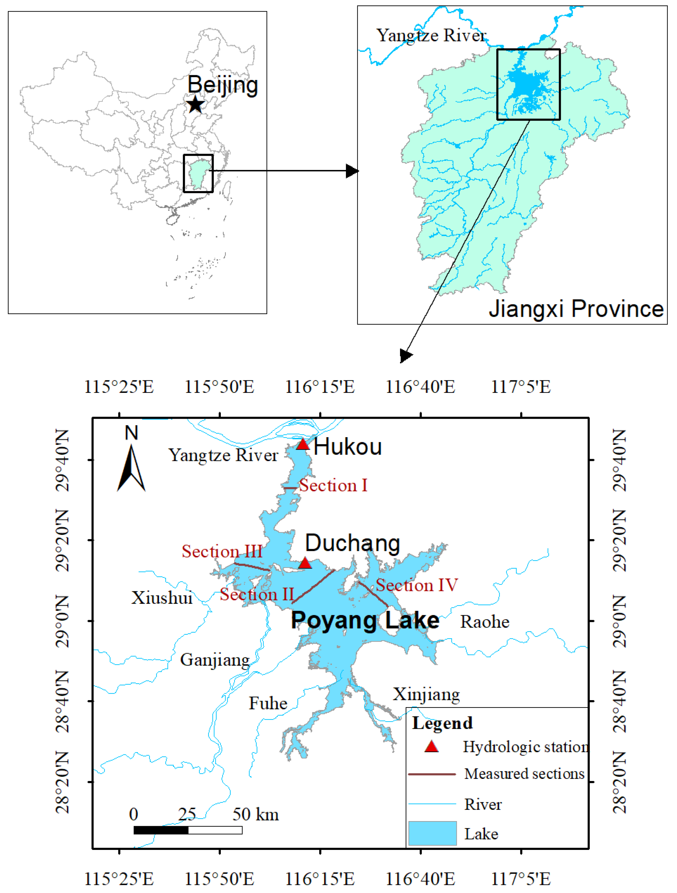
2.1. Study Area

Poyang Lake, with a surface area of over 4125 km2 and a water volume of 27.6 billion m3, is the largest freshwater lake in China. Poyang Lake is located in the north of Jiangxi Province and the south bank of the middle and lower reaches of the Yangtze River between 28°11′~29°51′ N and 115°49′~116°49′ E. The watershed of Poyang Lake covers an area of 162,225 km2, which accounts for about 97% of the total area of Jiangxi Province [37]. Poyang Lake is an important wetland in the world. It is one of the top ten ecological function reserves in China and one of the important ecological areas in the world; this is recognized by the World Wide Fund for Nature (WWFN).
The subtropical monsoon climate in this area gives rise to mild and humid weather, with an annual average temperature of 17.1 °C and an annual average precipitation measurement of 1570 mm. The water level of Poyang Lake shows significant seasonal changes due to seasonal variations in precipitation, as well as the alternation of flood and dry seasons in the upper reaches of the Yangtze River. Consequently, significant variations in the surface area of the lake can be noted during the year. During the flood season, the water level of Poyang Lake reaches the yearly maximum, together with a maximum surface area of over 4125 km2. During the dry season, the lake’s minimum surface area is only about 500 km2. In recent years, the hydrological situation of Poyang Lake has varied greatly since the Three Gorges Project (TGP), the largest water conservancy hub project in the world, came into operation in 2003.
As shown in Figure 1, water from rivers, including the Xiushui, Ganjiang, Fuhe, Xinjiang, and Raohe, flows through Poyang Lake into the Yangtze River. Poyang Lake is divided into two parts by Songmen Mountain. The southern part contains the main lake area where the lake is wide and shallow. The northern part contains the channel into the Yangtze River where the lake is narrow and deep. The whole lake tilts from the southeast to the northwest.

2.2. Materials

2.2.1. Global Surface Water Dataset

The GSW dataset contains maps of the location and temporal distribution of surface water on the global scale and provides statistics on the extent and change in the global water surfaces [33]. The dataset was produced by the European Commission’s Joint Research Centre (JRC) and Google using 4,453,989 scenes from Landsat 5, 7, and 8 acquired between 16 March 1984 and 31 December 2020. Each pixel in the mapping layers of the GSW dataset was individually classified into water/non-water using an expert system [33]. The GSW dataset maps different facets of the spatial and temporal distribution of surface water over the last 37 years and contains seven bands, including water cccurrence, seasonality, recurrence, transitions, etc. The GSW dataset can be accessed and used on the Google Earth Engine (GEE) platform (https://earthengine.google.com/ accessed on 1 August 2021).
The water occurrence thematic map in the GSW dataset contains the main supporting data for this study and acts as the base map of the final bottom topographic map. This water occurrence map, with a spatial resolution of 30 m, shows where surface water occurred between 1984 and 2020 and provides information concerning the overall water dynamics. The discrete value of each pixel in the water occurrence map ranges from 1 to 100, and it reflects the proportion (or frequency) of the pixel observed as water in all available Landsat observations without clouds and shadows from 1984 to 2020. The water occurrence in a month ( W O m o n t h ) can be calculated as follows [33]:
W O m o n t h =   W D m o n t h   V O m o n t h
where W D m o n t h and V O m o n t h refer to water detections and valid observations from the same months, respectively. The long-term overall surface water occurrence was obtained by averaging the results of all monthly W O m o n t h calculations.

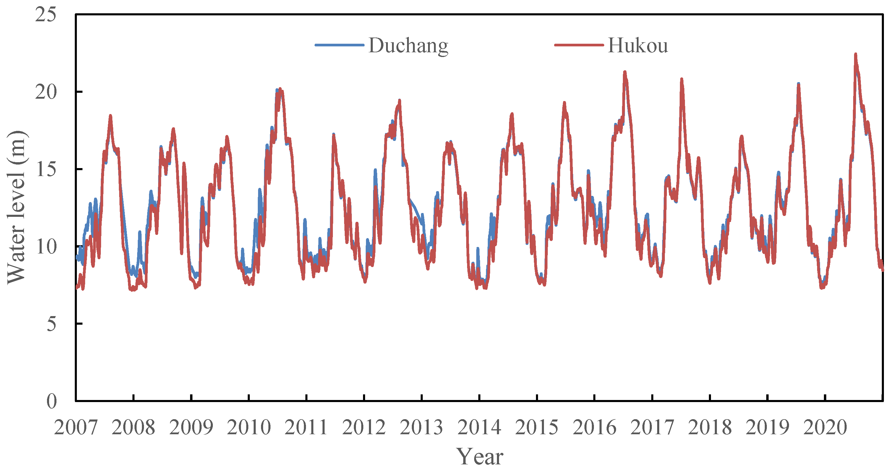
2.2.2. Lake Water Level Data

In this study, the daily water levels of Poyang Lake from the Hukou station and the Duchang station from 1993 to 2020 were used as the measured data. These water level data were calibrated against the elevation reference of Woosung Horizontal Zero (W.H.Z.) [38] and were downloaded from the National Water and Rainfall Information Network (http://xxfb.mwr.cn/ accessed on 1 July 2021). Water level data before 1993 are not available currently. The distributions of the hydrologic stations are shown in Figure 1.

2.2.3. Measured Lake Topographic Data
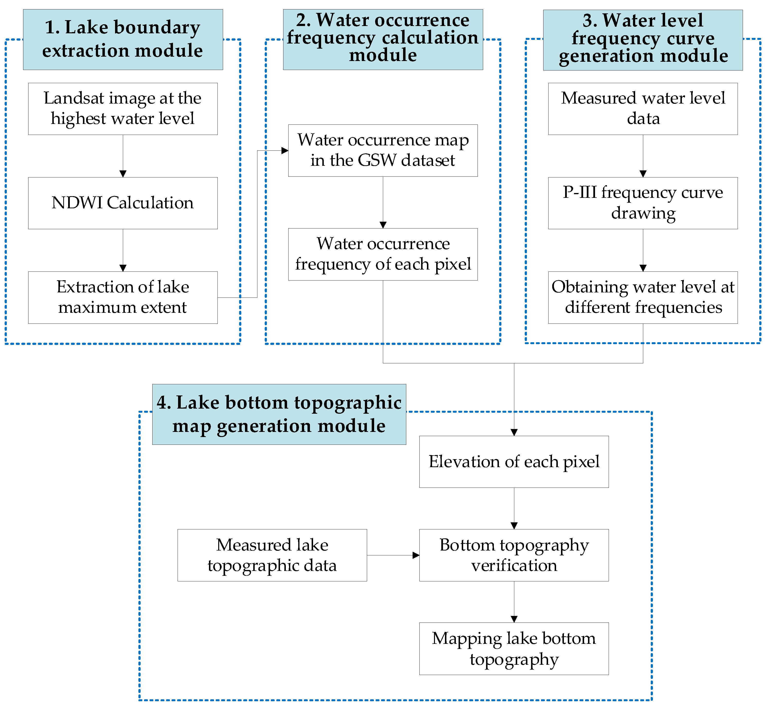
The measured topographic data of four sections of Poyang Lake in 2010 were used for verification in this paper. These topographic data were measured by digital depth sounder and GPS on a remote monitoring ship, and the measured points were arranged along the section every 100~2000 m. The topographic data, including the longitude, the latitude, and the elevation referenced against the W.H.Z. of the measured points, were obtained from the Jiangxi Hydrological Bureau, and the locations of the sections are shown in Figure 1.

2.3. Methods

In this study, a novel method for lake bottom topography mapping was proposed by combining the water occurrence map from the GSW dataset and the daily measured water level data. The core concept of this method can be described as follows: The water level at a specific time can be regarded as the elevation along the water/land boundary [17]. As the water level of a lake fluctuates over time, the bottom elevation within the lake’s dynamic inundation area can be derived continuously. Over a long temporal span, there exists a corresponding relationship between the water occurrence frequency and the bottom elevation. Bottoms with lower elevations may be inundated more frequently, while bottoms with higher elevations may be inundated less frequently. In other words, higher water occurrence frequency corresponds to a lower elevation, while lower water occurrence frequency corresponds to a higher elevation. Referring to the definition of hydrologic frequency in hydrology, we put forward the concept of lake water level frequency in this paper, which refers to the frequency at which the lake water level is higher than or equal to a specified elevation. As for any part of the lake bottom, if water occurred there more frequently, we can infer that it was inundated more frequently, which is to say that the water level was higher than its bottom elevation more frequently. Therefore, we can assume that the water level frequency is identical to the water occurrence frequency over a long period. If we pair the water level frequency with the water occurrence frequency and assign the water level (elevation) value to each pixel with the same frequency in the water occurrence map, then the bottom topographic map can be generated.
As some parts of the lake bottom are covered by water all the year round, the proposed method in this paper can only map the bottom topography of a lake’s dynamic inundation area, and the elevations of lake bottom covered by permanent water (locations with the water occurrence frequency of 100%) are still undetermined. In addition, the proposed method is mainly applicable to large lakes, whose inundation area varies greatly and whose water level changes rapidly in a year. For lakes with minor water level variations, this proposed method may not work well.
The method in this paper consists of four parts. The lake boundary extraction module (LBEM) is used to extract the maximum extent of the lake, namely, the inundation area when the lake reached its highest water level. The water occurrence frequency calculation module (WOFCM) retrieves the GSW dataset to obtain the water occurrence frequency of each pixel within the lake’s maximum inundation area. The water level frequency curve generation module (WLFCGM) is intended to generate a reasonable water level frequency curve of all the measured water level data using the P-III distribution function, which is a commonly used mathematical distribution in hydrologic statistics [39,40]. The lake bottom topographic map generating module (LBTMGM) is used to assign the elevation value to each pixel and generate the lake bottom topographic map by integrating the elevation value and coordinates of each pixel. A flowchart of this method is illustrated in Figure 2.
  • Lake boundary extraction module
Firstly, the Landsat image (Row = 121, Path = 40) acquired on the day when the lake reached its highest water level between 1984 and 2020 is downloaded from the U.S. Geological Survey (http://glovis.usgs.gov/ accessed on 1 June 2021). Then, the normalized difference water index (NDWI) method [41] is used to extract the boundary as the lake’s maximum extent. The NDWI proposed by McFeeters in 1996 aims at detecting surface waters in wetland environments [41]. It has been widely used to extract water from remote sensing images in recent years [42,43,44]. The NDWI can be calculated as follows:
NDWI = Green     NIR Green   +   NIR
where Green is the TOA reflectance value of the Green band (Band 2 for Landsat TM & ETM+ data, Band 3 for Landsat OLI data) and NIR is the TOA reflectance value of the near-infrared band (Band 4 for Landsat TM & ETM+ data, Band 5 for Landsat OLI data). The range of the NDWI is from −1 to 1. The threshold value of the lake water boundary is 0; the area with an NDWI greater than 0 is water surfaces; and the area with an NDWI less than or equal to 0 is non-water surfaces [41]. Finally, visual examination and manual modification were conducted on the extracted boundary.
2.
Water occurrence frequency calculation module
According to the lake’s maximum extent, the water occurrence frequency of pixels within the extent can be extracted from the water occurrence map in the GSW dataset, which represents the frequency with which water was present on the surface from 1984 to 2020 [33].
3.
Water level frequency curve generation module
In the WLFCGM, the historical measured water levels of the lake are firstly obtained, then the empirical frequency of each water level value is calculated, and the empirical points are generated. The P-III distribution function is utilized to draw the theoretical frequency curve. The theoretical frequency curve is adjusted according to the fitting degree between the empirical points and the theoretical frequency curve, and the final adjusted theoretical frequency curve is taken as the water level frequency curve of the lake.
(1)
Empirical frequency calculation
All of the lake’s measured water level values are arranged and numbered in a sequence in order from large to small (x1x2 ≥ ... xm ≥ ... ≥ xn), where x1 and xn represent the highest and lowest water level values of all the measured water level data (m), respectively; xm {xn, x1} represents a certain water level value in the sequence (m), n represents the total number of the measured water level data, and m {1, n} represents the sequence number of a certain water level value.
For a certain water level xm, the empirical frequency Pm (%) can be calculated by Equation (3):
P m = m n + 1  
where the empirical points are obtained by taking the empirical frequency Pm as the x-axis and the water level value xm as the y-axis on the Hazen probability paper.
(2)
P-III distribution function
The frequency density function of the P-III distribution curve is as follows:
f ( x ) = β α Γ ( α ) ( x a 0 ) α 1 e β ( x a 0 )   ( x   >   a 0 ,   α   >   0 ,   β   >   0 )
where a 0 represents location parameters (m) and β and α are scale parameters and shape parameters, respectively. They can be calculated as follows:
a 0 = x ¯ ( 1 2 C v C s )
α = 4 C s 2
β = 2 x ¯ C v C s
where x ¯ represents the mean of the water level sequence (m) and C v and C s represent the variation coefficient and skewness coefficient of the water level sequence, respectively.
(3)
Parameter estimation
The method of moments is used to estimate the three parameters of the P-III distribution function. The mean ( x ¯ ), variation coefficient ( C v ), and skewness coefficient ( C s ) can be calculated as follows:
x ¯ = 1 n   x i
C v = 1 n 1   ( x i x ¯ 1 ) 2
C s =   ( x i x ¯ 1 ) 3 ( n 3 ) C v 3
where xi (i {1, n}) represents each water level value in the sequence (m).
(4)
Curve fitting
The deviation coefficient ( Φ ) values corresponding to different frequencies (P), Cv, and Cs can be found from the Φ table of the P-III distribution function. The x values, namely the water level values to derive (m), corresponding to each frequency (P) under a certain Cv can be calculated according to Equation (11).
x = x ¯ ( 1 + C v Φ )
Draw the points (P, x) on the Hazen probability paper, and then connect these points with a smooth curve as the theoretical frequency curve. Adjust the values of Cv and Cs according to the fitting between the theoretical frequency curve and the empirical points until the curve fits well with the empirical points.
4.
Lake bottom topographic map generating module
The water level values in the water level frequency curve are stored in a frequency-elevation table. From 1% to 100%, each frequency value corresponds to an elevation (water level) value. The water cccurrence map is used as the base map. For each pixel in the water occurrence map, use the frequency value of the pixel to retrieve from the frequency-elevation table and receive the corresponding elevation value. Then, assign the derived elevation value to the pixel. Loop until all the pixels in the map are assigned; then, the lake bottom topographic map can be generated automatically in TIF format. These procedures are implemented automatically by coding with the Geospatial Data Abstraction Library (GDAL) in Python 2.7.
Based on the derived bottom topographic map, lake water volume can be estimated with a corresponding water level value using the “Surface Volume” function of the 3D Analyst Tool in ArcMap 10.8, and the lake inundation range can be extracted with a corresponding water level value using the “Reclass” function of the Spatial Analyst Tool in ArcMap 10.8.
The mean relative error (MRE) and the root mean square error (RMSE) are used to verify the derived results of lake bottom topography. The MRE (%) and RMSE (m) can be calculated as follows:
MRE = i = 1 N abs ( x i y i ) / y i N  
  RMSE = i = 1 N ( x i y i ) 2 N
where xi is the calculated value (m), yi is the true value (m), and n is the number of samples.

3. Results

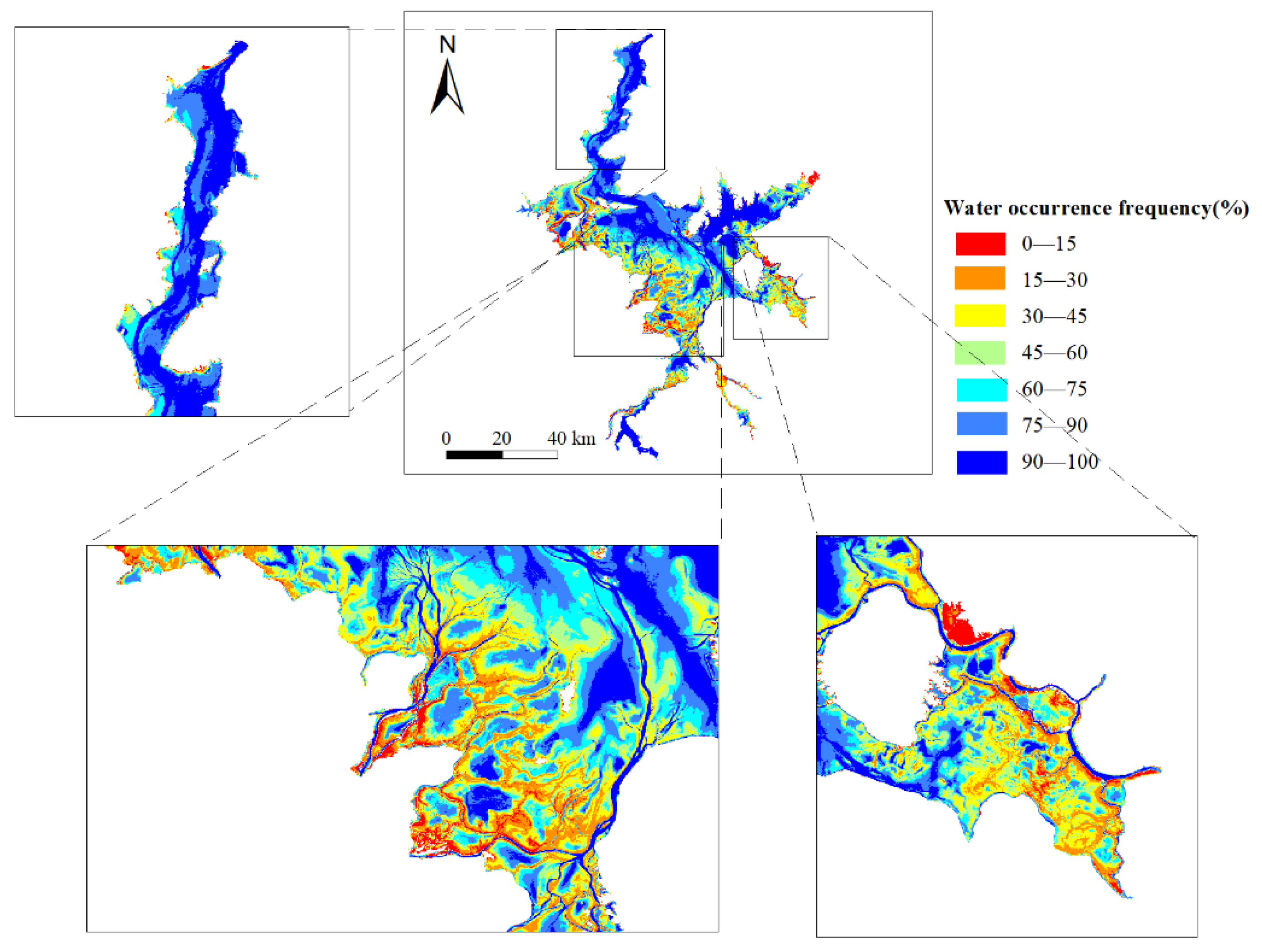
3.1. Water Occurrence Frequency of Poyang Lake

The highest water level of Poyang Lake from 1993 to 2020 occurred on 12 July 2020. The boundary of Poyang Lake on this day was extracted as the maximum extent of Poyang Lake. The water occurrence frequency of Poyang Lake was extracted from the water occurrence map of the GSW dataset, as shown in Figure 3. Percentages of each interval were counted, as shown in Figure 4. On the whole, the water occurrence frequency in the northern part of Poyang Lake is higher than that in the southern part. By adding up the area of all the pixels with a frequency equal to or greater than 1%, we can calculate that the maximum area of Poyang Lake is 4187.79 km2. Similarly, the lake area varied from 575.76 to 4187.79 km2 from 1984 to 2020. The area with a water occurrence frequency greater than or equal to 95% is 734.9 km2, which accounts for 17.5% of the total area of Poyang Lake, indicating that 17.5% of the lake is almost covered by water all the year round. The area with a water occurrence frequency of 91~100% is 1351.43 km2, which accounts for 32.3% of the total area of Poyang Lake. The area with a water occurrence frequency of 51~100% is 3104.95 km2, which accounts for 74.1% of the total area of Poyang Lake. The area with a water occurrence frequency less than 50% is 1082.84 km2, which accounts for 25.9% of the total area of Poyang Lake, indicating that 25.9% of the lake bed is dry for half of the time.

3.2. Water Level Frequency Curve of Poyang Lake

A comparison of water level records in the Hukou station and the Duchang station from 2007 to 2020 is shown in Figure 5. The lowest water levels of Poyang Lake ever recorded in the Duchang station and the Hukou Station were 7.47 m and 7.15 m, respectively, occurring on 1 February 2014 and 21 December 2007, respectively, and the highest water levels ever recorded in these two stations were 22.42 m and 22.49 m, respectively, both occurring on 12 July 2020. As can be seen in Figure 5, the seasonal variations in Poyang Lake’s water level during a year are significant. From January to February, the water level rises gradually; the annual highest water level mostly occurs between June and July, and the water level gradually decreases from July to January of the next year. In the dry season, the water level of the Duchang station is higher than that of the Hukou station, and the maximum height difference is 2.73 m, while there is little difference between the water level of the Duchang station and the Hukou station in the flood season. Under normal circumstances, Poyang Lake flows into the Yangtze River from south to north, and, therefore, the water level in the south is higher than that in the north. However, in the flood season, due to the backwater of the Yangtze River [45], the water flow reverses from north to south, and the water level of the whole lake is almost the same.
The P-III distribution function was used to generate a reasonable water level frequency distribution curve. The mean value, variation coefficient, and skewness coefficient of the water level series calculated by the method of moments were used as the initial values, and then, these statistical parameters were continuously adjusted by the curve fitting method until the theoretical frequency curve fits well with the empirical points. The adjusted water level frequency curves of the Hukou station and the Duchang station are shown in Figure 6. The water levels corresponding to the water level frequency, ranging from 1% to 100%, were calculated, as shown in Figure 7. It can be seen that a higher water level frequency corresponds to a lower water level, whereas a lower water level frequency corresponds to a higher water level. When the frequency is greater than 30%, the water levels of the Duchang station are greater than those of the Hukou station. When the frequency is less than 30%, there are small differences between the water levels of the Hukou station and the Duchang station.

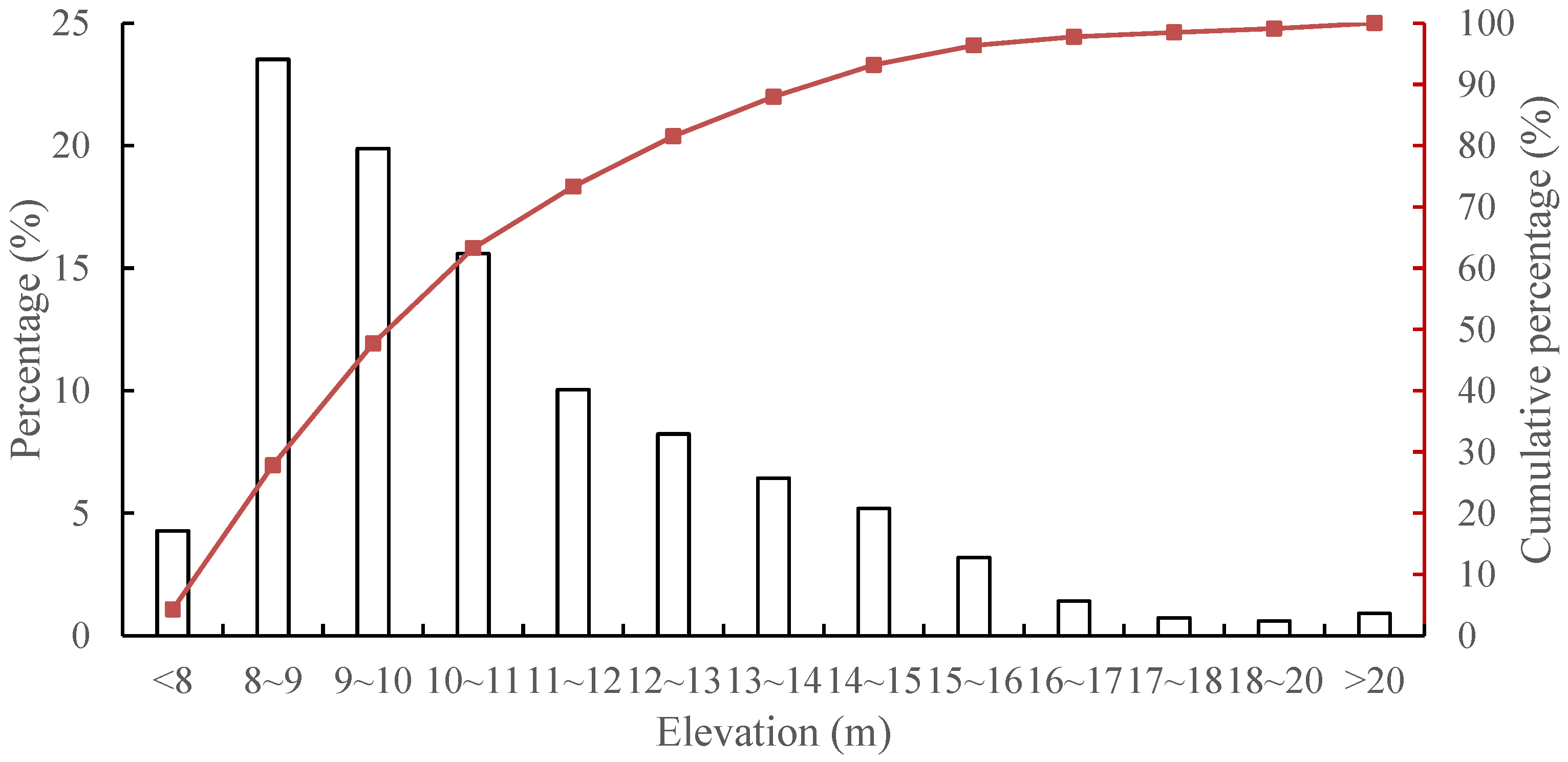
3.3. Bottom Topographic Map of Poyang Lake

The water level frequency in the northern part of Poyang Lake was determined according to the water level sequence of the Hukou station, and the water level frequency in the southern part of the lake was determined according to the water level sequence of the Duchang Station. Based on the water occurrence frequency and the water level frequency curve of Poyang Lake, the elevation of each pixel within the water occurrence map was assigned according to elevation values in the water level frequency curve, and the bottom topographic map of Poyang Lake was drawn, as shown in Figure 8. The spatial resolution of the derived bottom topographic map is 30 m, and the bottom elevation is against the elevation reference of W.H.Z. The entire bottom elevation of Poyang Lake is lower than 23.5 m, showing a decreasing trend from south to north. At the northern outlet and the center of the lake, the elevation is mostly lower than 10 m, while the elevation of the southern lake area is mostly 10~23.5 m. As can be seen from the elevation distribution histogram in Figure 9, the area with bottom elevations lower than 13 m accounts for 81.5% of the total area of Poyang Lake, among which the area with elevations between 8~9 m accounts for 59.0%. The area with bottom elevations higher than 15 m accounts for only 6.83% of the total area. It should be pointed out that the method in this paper can only map the lake bottom topography with an elevation higher than the lowest water level ever recorded. For the part of the lake which is covered by water all the year round, namely the pixels with a water occurrence frequency of 100%, we can not determine accurate elevation values.

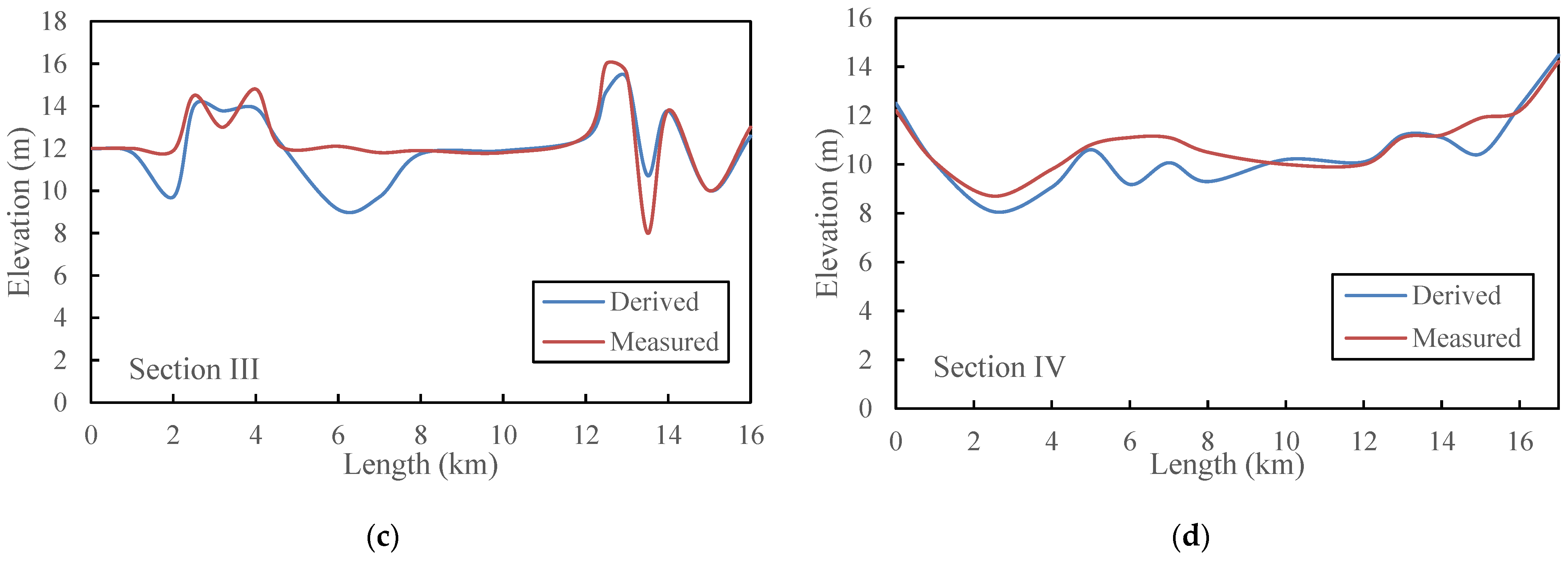
3.4. Verification of the Proposed Method

The accuracy of the derived topographic data was verified according to the measured elevation data of four sections of the Poyang Lake. Based on the longitude and latitude of the measured points, these points were added as a layer in ArcMap 10.8 using the WGS 1984 Geographic Coordinate System and overlapped on the derived bottom topographic map. Then, the measured elevations and the elevations in the derived topographic map can be compared. The comparison of the measured and derived elevation values of Sections I to IV is shown in Figure 10 and Figure 11. It can be seen that the derived elevation values fit well with the measured values. The absolute error is mostly less than 0.5 m, and the MRE and RMSE of all the four sections are 7.4% and 0.99 m, respectively, indicating that the method proposed in this paper has high accuracy and can be used to reflect the bottom topography of the lake. However, large relative differences can be observed in Section I and Section III, which are located in the northern outlet, as shown in Table 1. The MRE and RMSE of Section I are 17.24% and 1.37 m, respectively, and the MRE and RMSE of Section III are 7.14% and 1.27 m, respectively. Since the water occurrence frequency used in this paper covers 37 years of data, it may indicate changes in lake bottom topography at the northern outlet caused by sedimentation, scouring, and human activities between 1984 and 2020.

4. Discussion

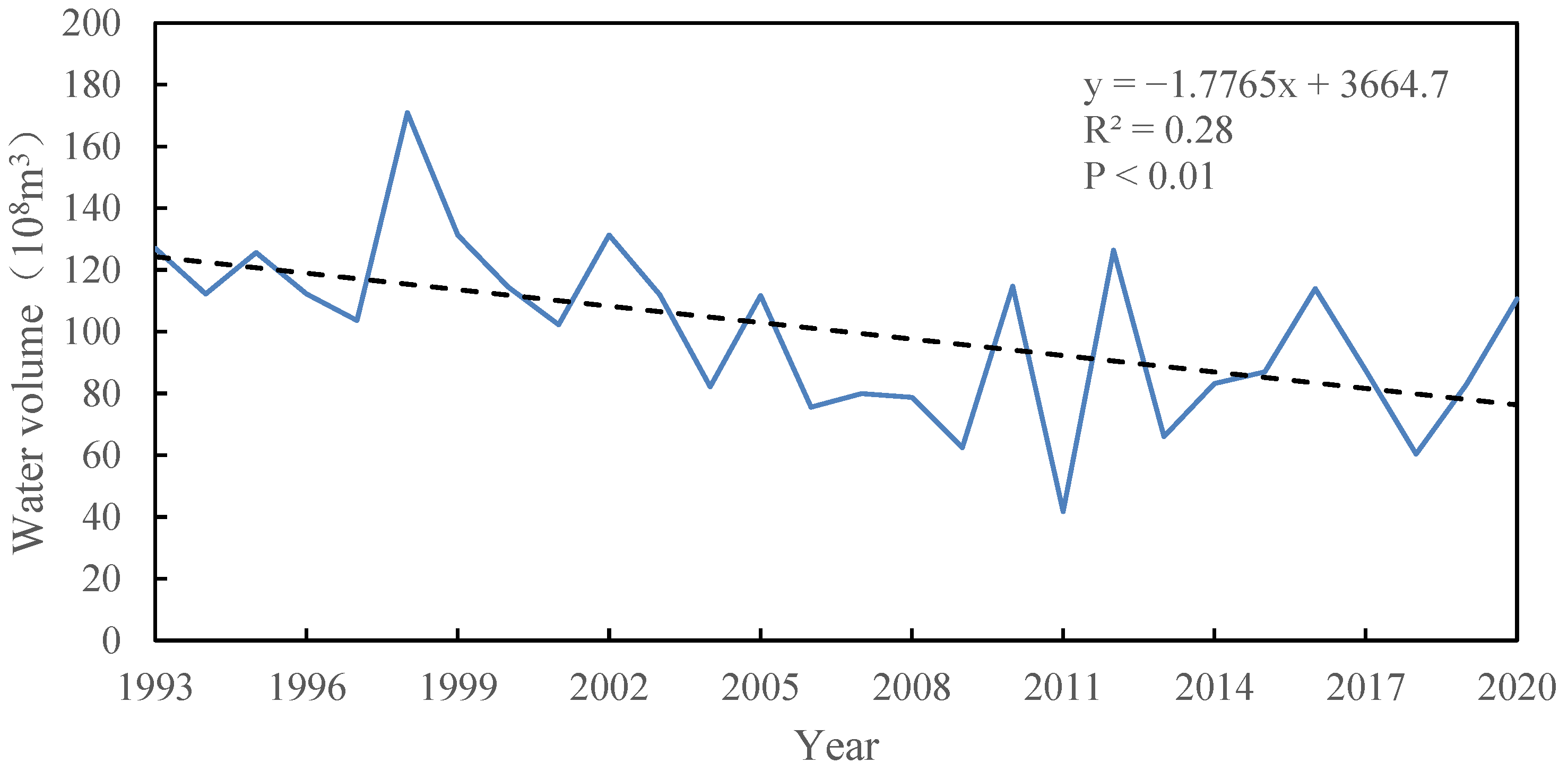
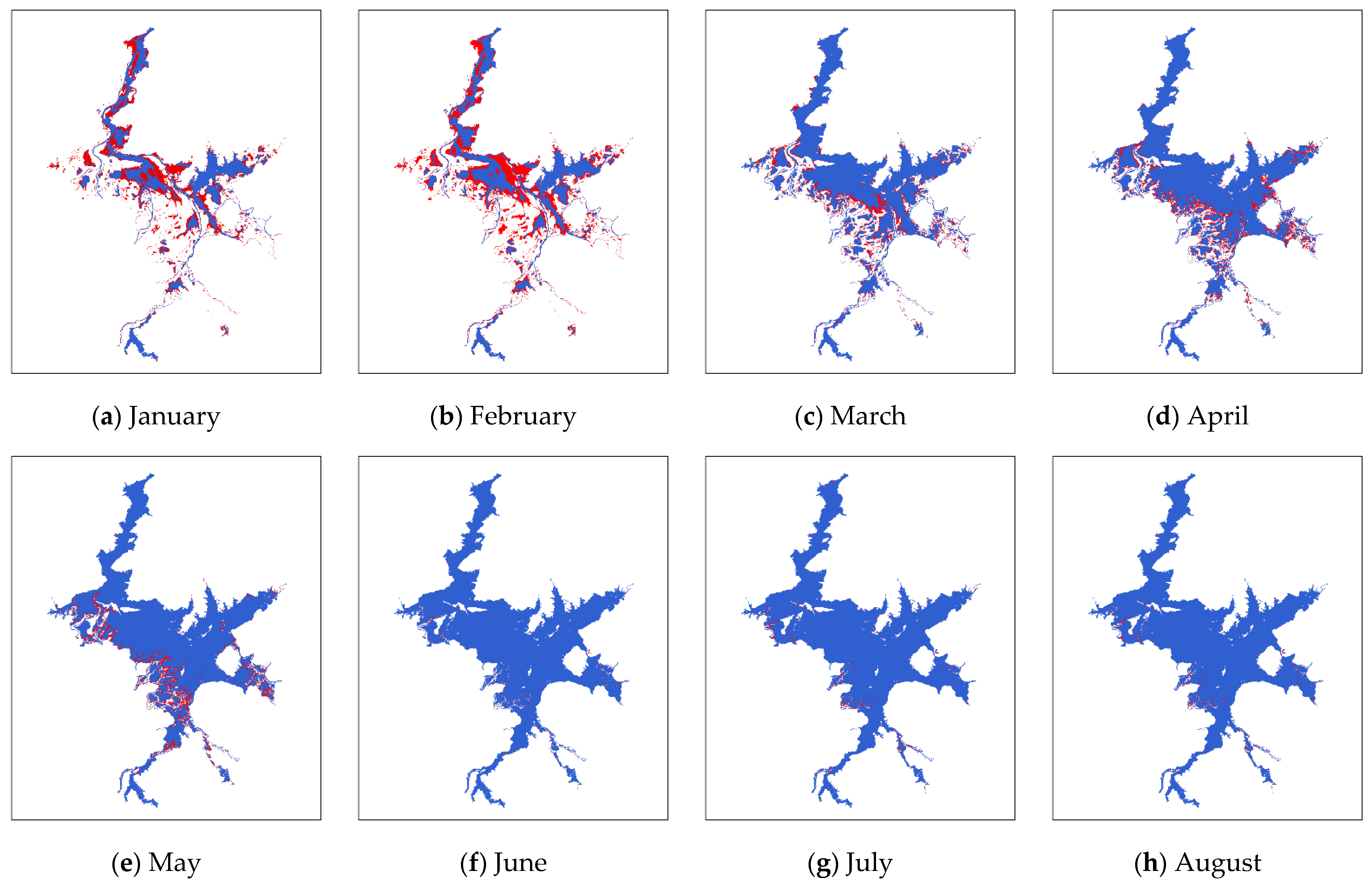
4.1. The Spatiotemporal Variations of Poyang Lake Based on the Derived Bottom Topography

Based on the bottom topographic map drawn in this paper and the water level data, the corresponding inundation range and water volume of the lake can be obtained efficiently with fewer procedures. Based on the annual average water levels from 1993 to 2020, the inter-annual variations of Poyang Lake’s water volume were calculated, as shown in Figure 12. It can be seen that the water volume of Poyang Lake shows a significant decreasing trend during the past 28 years, with an average decreasing rate of 1.78 × 10⁸ m3/yr. The average annual water volume before the TGP (1993~2002) was 123.08 × 10⁸ m3, and the average annual water volume after the TGP (2003~2020) was 87.61 × 10⁸ m3, 28.8%, which is lower than that before the TGP.
Based on the monthly average water levels from 1993 to 2020, the monthly variations of Poyang Lake’s inundated area before and after the TGP are exhibited in Figure 13. The area of Poyang Lake varied significantly during different seasons within a year. The monthly average maximum area is 4070.1 km2 in July, and the monthly average minimum area is 1149.1 km2 in January, as shown in Figure 14. Compared with the area before the TGP, the area decreased every month after the TGP. The monthly differences in area are more obvious in the dry season, during which the area decreased by 921.3 km2 in February. In the flood season, there were little differences in Poyang Lake’s area before and after the TGP.
The spatiotemporal dynamics of Poyang Lake were influenced by many factors, including climate changes, the TGP regulation, human activities, etc. In recent years, a decrease in precipitation directly affected runoff into the lake, which resulted in a reduction in the water volume and shrinkage of the area [46]. In addition, the impoundment of the TGP, in June 2003, changed the hydrological relationship between the Yangtze River and Poyang Lake, resulting in a decline in both the flow and water level in the lower reaches of the river [17]. Besides, human activities, such as heavy sand mining and water withdrawal, have also contributed to the reduction in lake water volume [47]. However, the main driving forces of Poyang Lake’s spatiotemporal variations are still unclear, and quantitative analysis of the contribution of each factor is still insufficient, thus requiring further research in the future.

4.2. Advantages of the Proposed Method

Lake bottom topography is a fundamental parameter for characterizing lakes and is also highly associated with variations in water levels and volumes [18]. Consequently, it is necessary to obtain accurate and timely information on lake bottom topography. However, the scarcity of publicly available datasets on lake bottom topography makes it difficult for us to carry out research relevant to lakes or have a further understanding of the lake dynamics and the hydrologic cycle [25]. Traditional methods rely on large measuring instruments and are of high-cost and intensive labor, which limits their use at a larger scale. Our study provides an advanced and feasible approach to map the lake bottom topography without in situ survey. By taking advantage of the rapid change in water level in the lake’s dynamic inundation area, the water level frequency curve was drawn, the relationship between the lake bottom elevation and the water occurrence frequency was established, and finally the bottom topographic map was generated.
Mapping lake bottom topography with remote sensed data has gained much attention over the past few years. Some publications focused on bottom topography estimation by combining satellite altimetry data with satellite image data. Compared with these approaches, the proposed method has the advantages of less computation, higher accuracy, and easier data acquisition. The GSW dataset maps and offers statistics on the spatiotemporal dynamics of global surface water over the past 37 years with a spatial resolution of 30 m, which covers 99.95% of the landmass [33]. This means that with sufficient water level data available, we can obtain the bottom topographic data of lakes with significant variations in different regions of the world. In addition, the classifier of the GSW dataset has been proven robust and accurate, with less than 1% of false water detections and less than 5% omissions [33]. Therefore, we can infer that the influence of classification errors in the GSW dataset on the final bottom topography is very limited.

4.3. Limitations of the Proposed Method

Some limitations exist in the proposed method.
Firstly, the proposed method does not fully apply to all kinds of lakes. This method takes advantage of the feature that the rapid change in water level in a lake’s dynamic inundation area leads to a different water occurrence frequency. Therefore, this method is mainly applicable to large lakes with periodically significant water level changes. For lakes with minor spatiotemporal variations, e.g., lakes whose area changes a little and whose water level fluctuates within a small range during a year, it seems that this method does not make much sense, as a large part of these lake bottoms are covered by permanent water. The derived bottom topography using this method may only cover a tiny fraction of the whole lake bottom.
Secondly, the proposed method cannot map the bottom topography of an entire lake. It can only map the bottom topography within a lake’s dynamic inundation area. The measured water level values are used to represent the lake bottom elevations in this study. As some parts of the lake bottom are covered by water throughout the year, we cannot obtain the specific elevation value of the bottoms covered by permanent water, and we can only determine that the elevation of these bottoms is lower than the lowest water level ever recorded. From this perspective, the method in this paper may be more helpful for shallow lakes.
Thirdly, we established the relationship between the lake bottom topographic elevation and water occurrence frequency from 1984 to 2020 based on the assumption that the lake bottom elevation was constant over time, which could inevitably lead to errors if the lake bottom topography changes significantly. Previous studies [17,48,49] have shown that significant inter-annual variabilities have been found in part of Poyang Lake’s bottom topography in recent decades due to the combined influence of climate change and human activities (sand dredging, the TGP, etc.). This may explain the large errors between the derived elevation and the measured elevation at Sections I and III in the case study.

4.4. Application Prospect

It has been proven that the novel method proposed in this paper enriches the mapping means of lake bottom topography and provides strong technical support for the analysis of lake hydrological features. This study demonstrates the effectiveness of combining the GSW dataset and the measured water level data on lake bottom topography estimation, which is conducive to the application of remote sensing in the field of hydrology. Good agreements in the verification indicate that our method has the potential to become a useful tool with broad application prospect and can be further applied to monitor and analyze the long-term dynamic changes in water depth and lake water volume.
In some remote areas, such as the Tibetan Plateau, there are only a few hydrologic stations. The scarcity and discontinuity of measured water levels makes it difficult for the extension and application of the lake bottom topography mapping method proposed in this paper. Fortunately, the development of satellite altimetry technology provides a fast and effective evaluation method for monitoring and analyzing lake water level variations [50,51,52,53]. For lakes with incomplete water level data, we can make full use of the state-of-the-art altimetry missions, including ICESat-2, Sentinel-3 & 6, and SWOT (targeted for launch later this year), in order to obtain water level observation results with high accuracy. Then, we can achieve a long-term water level series based on the empirical relationship between the area and water level [54] or by interpolating between the derived water levels [55].
With the development of remote sensing technology and the improvement of the spatial and temporal resolutions of remote sensed data, a series of surface water data sets have been generated and updated, including the Global Lakes and Wetlands Database (GLWD) [56], the Hydroweb Database (HD) [57], the Database for Hydrological Time Series of Inland Waters (DAHITI) [58], the Global Reservoir and Dam Database (GRanD) [59], etc. These data sets provide the basic attributes of surface water, including geographical location, range, area, water level, etc. However, few of them include lake bottom topography. The method proposed in this paper can be widely used to map the bottom topography of lakes, especially the unmeasured areas, and can enrich regional and even global lake bottom topography data sets.

5. Conclusions

In this paper, we proposed a novel method to map lake bottom topography using the GSW dataset and measured water level data. Concretely, this method consists of four parts. First, the lake’s maximum inundation area, corresponding to the highest water level, is extracted from the Landsat image using the NDWI method. Second, the water occurrence frequency of each pixel within the lake’s maximum inundation area is extracted from the GSW dataset. Then, the P-III distribution function is used to draw the water level frequency curve of all the measured water levels. Finally, elevation values from the water level frequency curve are assigned to pixels with the same frequency in the water occurrence map, and the bottom topographic map of the lake is generated.
As Poyang Lake is the largest freshwater lake in China and is a typical lake with great seasonal variations, we established a test case for bottom topography mapping over Poyang Lake. The derived lake bottom topography was verified by four measured sections of Poyang Lake, and the results demonstrated that the proposed method was feasible and could well reflect the bottom topography of Poyang Lake. Most of the absolute errors were less than 0.5 m, and the MRE and RMSE of all the four sections were 7.4% and 0.99 m, respectively.
The proposed method provides a reliable alternative for mapping lake bottom topography, with the advantages of simple calculation, convenient data acquisition, and high efficiency. However, the proposed method also has some limitations. The method in this paper is more suitable for large lakes with seasonal inundation area variations and significant water level changes. Besides, the method cannot map the bottom elevation of the whole lake as permanent water exists in the lake bottom. In summary, through the combination of long-term remote sensed data and measured data, the proposed method with good robustness and high accuracy has a promising application prospect and can provide strong technical support for the analysis of lake hydrological features.

Author Contributions

Conceptualization, Y.L. and W.Y.; methodology, Y.L. and L.M.; software, W.Y.; validation, Y.L., W.Y. and Z.Z.; investigation, J.L.; data curation, Z.Z.; writing—original draft preparation, Y.L. and W.Y.; writing—review and editing, Y.L., W.Y., J.L., Z.Z. and L.M.; supervision, L.M.; project administration, Y.L. and L.M.; funding acquisition, L.M. All authors have read and agreed to the published version of the manuscript.

Funding

This work was funded by the National High-Resolution Earth Observation System Projects (civil part): Hydrological monitoring system by high spatial resolution remote sensing image (second phase) (Grant No.08-Y30F02-9001-20/22) and the National Key Research and Development Program of China (No.2021YFB3900603).

Institutional Review Board Statement

Not applicable.

Informed Consent Statement

Not applicable.

Data Availability Statement

Not applicable.

Acknowledgments

We thank the JRC and Google for providing the GSW dataset and the National Water and Rainfall Information Network for providing water level data. We also thank the anonymous reviewers for their detailed comments and suggestions.

Conflicts of Interest

The authors declare no conflict of interest.

References

  1. Verpoorter, C.; Kutser, T.; Seekell, D.A.; Tranvik, L.J. A global inventory of lakes based on high-resolution satellite imagery. Geophys. Res. Lett. 2014, 41, 6396–6402. [Google Scholar] [CrossRef]
  2. Lee, H.; Durand, M.; Jung, H.C.; Alsdorf, D.; Shum, C.K.; Sheng, Y. Characterization of surface water storage changes in Arctic lakes using simulated SWOT measurements. Int. J. Remote Sens. 2010, 31, 3931–3953. [Google Scholar] [CrossRef]
  3. Fang, Y.; Li, H.; Wan, W.; Zhu, S.; Wang, Z.; Hong, Y.; Wang, H. Assessment of Water Storage Change in China’s Lakes and Reservoirs over the Last Three Decades. Remote Sens. 2019, 11, 1467. [Google Scholar] [CrossRef] [Green Version]
  4. Gao, J. Bathymetric mapping by means of remote sensing: Methods, accuracy and limitations. Prog. Phys. Geogr. 2009, 33, 103–116. [Google Scholar] [CrossRef]
  5. Allen, S.E. On subinertial flow in submarine canyons: Effect of geometry. J. Geophys. Res. Ocean. 2000, 105, 1285. [Google Scholar] [CrossRef]
  6. Dawe, J.T.; Allen, S.E. Solution convergence of flow over steep topography in a numerical model of canyon upwelling. J. Geophys. Res. Ocean. 2010, 115. [Google Scholar] [CrossRef] [Green Version]
  7. Sima, S.; Tajrishy, M. Using satellite data to extract volume–area–elevation relationships for Urmia Lake, Iran. J. Great Lakes Res. 2013, 39, 90–99. [Google Scholar] [CrossRef]
  8. Qiao, B.J.; Zhu, L.P.; Wang, J.B.; Ju, J.T.; Ma, Q.F.; Huang, L.; Chen, H.; Liu, C.; Xu, T. Estimation of lake water storage and changes based on bathymetric data and altimetry data and the association with climate change in the central Tibetan Plateau. J. Hydrol. 2019, 578, 124052. [Google Scholar] [CrossRef]
  9. Yang, F.; Su, D.; Yue, M.; Feng, C.; Yang, A.; Wang, M. Refraction Correction of Airborne LiDAR Bathymetry Based on Sea Surface Profile and Ray Tracing. IEEE Trans. Geoence Remote Sens. 2017, 55, 6141–6149. [Google Scholar] [CrossRef]
  10. Kiss, T.; Sipos, G. Braid-scale channel geometry changes in a sand-bedded river: Significance of low stages. Geomorphology 2007, 84, 209–221. [Google Scholar] [CrossRef]
  11. Kurowski, M.; Thal, J.; Damerius, R.; Korte, H.; Jeinsch, T. Automated Survey in Very Shallow Water using an Unmanned Surface Vehicle—ScienceDirect. IFAC-PapersOnline 2019, 52, 146–151. [Google Scholar] [CrossRef]
  12. Zwolak, K.; Wigley, R.; Bohan, A.; Zarayskaya, Y.; Abou-Mahmoud, M.E.E. The Autonomous Underwater Vehicle Integrated with the Unmanned Surface Vessel Mapping the Southern Ionian Sea. The Winning Technology Solution of the Shell Ocean Discovery XPRIZE. Remote Sens. 2020, 12, 1344. [Google Scholar] [CrossRef] [Green Version]
  13. Flener, C.; Lotsari, E.; Alho, P.; Kyhk, J. Comparison of empirical and theoretical remote sensing based bathymetry models in river environments. River Res. Appl. 2012, 28, 118–133. [Google Scholar] [CrossRef]
  14. Senet, C.M.; Seemann, J.; Flampouris, S.; Ziemer, F. Determination of Bathymetric and Current Maps by the Method DiSC Based on the Analysis of Nautical X-Band Radar Image Sequences of the Sea Surface (November 2007). IEEE Trans. Geosci. Remote Sensing. 2008, 46, 2267–2279. [Google Scholar] [CrossRef]
  15. Gao, H. Satellite remote sensing of large lakes and reservoirs: From elevation and area to storage. Wiley Interdiscip. Rev. Water 2015, 2, 147–157. [Google Scholar] [CrossRef]
  16. Gao, L.; Liao, J.; Shen, G. Monitoring lake-level changes in the Qinghai-Tibetan Plateau using radar altimeter data (2002–2012). J. Appl. Remote Sens. 2013, 7, 073470. [Google Scholar] [CrossRef]
  17. Feng, L.; Hu, C.; Chen, X.; Li, R.; Tian, L.; Murch, B. MODIS observations of the bottom topography and its inter-annual variability of Poyang Lake. Remote Sens. Environ. 2011, 115, 2729–2741. [Google Scholar] [CrossRef]
  18. Cretaux, J.F.; Abarca-Del-Rio, R.; Berge-Nguyen, M.; Arsen, A.; Drolon, V.; Clos, G.; Maisongrande, P. Lake Volume Monitoring from Space. Surv. Geophys. 2016, 37, 269–305. [Google Scholar] [CrossRef] [Green Version]
  19. Lei, Z.; Xianyou, M.; Honglan, J.I.; Baosen, Z. Research on water depth inversion in reservoir area based on multi band remote sensing data. J. Hydraul. Eng. 2018, 49, 639–647. [Google Scholar]
  20. Wang, J.; Chen, M.; Zhu, W.; Hu, L.; Wang, Y. A Combined Approach for Retrieving Bathymetry from Aerial Stereo RGB Imagery. Remote Sens. 2022, 14, 760. [Google Scholar] [CrossRef]
  21. Randazzo, G.; Barreca, G.; Cascio, M.; Crupi, A.; Fontana, M.; Gregorio, F.; Lanza, S.; Muzirafuti, A. Analysis of Very High Spatial Resolution Images for Automatic Shoreline Extraction and Satellite-Derived Bathymetry Mapping. Geosciences 2020, 10, 172. [Google Scholar] [CrossRef]
  22. Kim, J.S.; Baek, D.; Seo, I.W.; Shin, J. Retrieving shallow stream bathymetry from UAV-assisted RGB imagery using a geospatial regression method. Geomorphology 2019, 341, 102–114. [Google Scholar] [CrossRef]
  23. Shen, X.; Ouyang, Z.; Leeuw, J.D. Constructing A DEM of Baiyang Lake Area from A Series of Landsat Images. Geogr. Geo-Inf. Sci. 2005, 21, 16–19. [Google Scholar]
  24. Duan, Z.; Bastiaanssen, W.G.M. Estimating water volume variations in lakes and reservoirs from four operational satellite altimetry databases and satellite imagery data. Remote Sens. Environ. 2013, 134, 403–416. [Google Scholar] [CrossRef]
  25. Changming, Z.; Xin, Z.; Ming, L.; Jiancheng, L. Lake Storage Change Automatic Detection by Multi-source Remote Sensing without Underwater Terrain Data. Acta Geod. Et Cartogr. Sin. 2015, 44, 309. [Google Scholar]
  26. Specht, M.; Specht, C.; Lewicka, O.; Makar, A.; Dbrowski, P.S. Study on the Coastline Evolution in Sopot (2008-2018) Based on Landsat Satellite Imagery. J. Mar. Sci. Eng. 2020, 8, 464. [Google Scholar] [CrossRef]
  27. Xu, N.; Ma, Y.; Zhou, H.; Zhang, W.; Zhang, Z.; Wang, X.H. A Method to Derive Bathymetry for Dynamic Water Bodies Using ICESat-2 and GSWD Data Sets. IEEE Geosci. Remote Sens. Lett. 2020, 19, 1–5. [Google Scholar] [CrossRef]
  28. Ma, Y.; Xu, N.; Liu, Z.; Yang, B.; Yang, F.; Wang, X.H.; Li, S. Satellite-derived bathymetry using the ICESat-2 lidar and Sentinel-2 imagery datasets. Remote Sens. Environ. 2020, 250, 112047. [Google Scholar] [CrossRef]
  29. Fair, Z.; Flanner, M.; Brunt, K.M.; Fricker, H.A.; Gardner, A. Using ICESat-2 and Operation IceBridge altimetry for supraglacial lake depth retrievals. Cryosphere 2020, 14, 4253–4263. [Google Scholar] [CrossRef]
  30. Wang, J.; Zhu, L.; Daut, G.; Ju, J.; Lin, X.; Wang, Y.; Zhen, X. Investigation of bathymetry and water quality of Lake Nam Co, the largest lake on the central Tibetan Plateau, China. Limnology 2009, 10, 149–158. [Google Scholar] [CrossRef]
  31. Li, C.Y.; Sun, B.; Gao, Z.Y.; Zhang, S. Retrieval model of water depth in Hulun Lake using multi-spectral remote sensing. Shuili Xuebao/J. Hydraul. Eng. 2011, 42, 1423–1431. [Google Scholar]
  32. Bagheri, S.; Stein, M.; Dios, R. Utility of hyperspectral data for bathymetric mapping in a turbid estuary. Int. J. Remote Sens. 1998, 19, 1179–1188. [Google Scholar] [CrossRef]
  33. Pekel, J.F.; Cottam, A.; Gorelick, N.; Belward, A.S. High-resolution mapping of global surface water and its long-term changes. Nature 2016, 540, 418–422. [Google Scholar] [CrossRef] [PubMed]
  34. Busker, T.; de Roo, A.; Gelati, E.; Schwatke, C.; Adamovic, M.; Bisselink, B.; Pekel, J.-F.; Cottam, A. A global lake and reservoir volume analysis using a surface water dataset and satellite altimetry. Hydrol. Earth Syst. Sci. 2019, 23, 669–690. [Google Scholar] [CrossRef] [Green Version]
  35. Xu, N.; Ma, X.; Ma, Y.; Zhao, P.; Yang, J.; Wang, X.H. Deriving Highly Accurate Shallow Water Bathymetry From Sentinel-2 and ICESat-2 Datasets by a Multitemporal Stacking Method. IEEE J. Sel. Top. Appl. Earth Obs. Remote Sens. 2021, 14, 6677–6685. [Google Scholar] [CrossRef]
  36. Lian, F.; Hu, C.; Chen, X.; Cai, X.; Tian, L.; Gan, W. Assessment of inundation changes of Poyang Lake using MODIS observations between 2000 and 2010. Remote Sens. Environ. 2012, 121, 80–92. [Google Scholar]
  37. Shankman, D.; Liang, Q. Landscape Changes and Increasing Flood Frequency in China’s Poyang Lake Region. Prof Geogr. Prof. Geogr. 2003, 55, 434–445. [Google Scholar] [CrossRef]
  38. Woosung Horizontal Zero. Available online: http://baike.baidu.com/view/173481.htm (accessed on 6 March 2022).
  39. Weiya, M. Study on The Application of Excel to Pearson Type III Distribution Multi-samples Parameter Estimation in Hydrology. Agric. Technol. 2005, 25, 93–95. [Google Scholar]
  40. Lin, L.; Wang, L. Estimation of Annual Maximum Diurnal Precipitation for Reappearance Periods with Pearson-III Distribution. Meteorol. Sci. Technology. 2005, 33, 314–317. [Google Scholar]
  41. McFeeters, S.K. The use of the normalized difference water index (NDWI) in the delineation of open water features. Int. J. Remote Sens. 1996, 17, 1425–1432. [Google Scholar] [CrossRef]
  42. Wang, B.; Miao, F.; Chen, J. The construction and application of normalized difference water index (NDWI) based on the ASTER image. Sci. Surv. Mapp. 2008, 33, 177–179. [Google Scholar]
  43. Zhang, J.; Kuligowski, R.J.; Parihar, J.S.; Guo, W.; Saito, G. Quantitative retrieval of crop water content under different soil moistures levels. Proc. Spie 2006, 6411, 85–93. [Google Scholar]
  44. Gautam, V.K.; Gaurav, P.K.; Murugan, P.; Annadurai, M. Assessment of Surface Water Dynamicsin Bangalore Using WRI, NDWI, MNDWI, Supervised Classification and K-T Transformation. Aquat. Procedia 2015, 4, 739–746. [Google Scholar] [CrossRef]
  45. Shankman, D.; Keim, B.D.; Song, J. Flood frequency in China’s Poyang Lake region: Trends and teleconnections. Int. J. Climatol. 2006, 26, 1255–1266. [Google Scholar] [CrossRef] [Green Version]
  46. Mei, X.; Dai, Z.; Du, J.; Chen, J. Linkage between Three Gorges Dam impacts and the dramatic recessions in China’s largest freshwater lake, Poyang Lake. Sci. Rep. 2015, 5, 18197. [Google Scholar] [CrossRef] [PubMed] [Green Version]
  47. Min, Q.; Zhan, L. Characteristics of low-water changes in Lake Poyang during 1952-2011. J. Lake Sci. 2012, 24, 675–678. [Google Scholar]
  48. Xingwang, W.G.L.Y.F. Bottom topography change patterns of the Lake Poyang and their influence mechanisms in recent 30 years. J. Lake Sci. 2015, 27, 1168–1176. [Google Scholar]
  49. Jiuwei, H.; Dunyin, W.; Rongfang, L. Analysis of Fluvial Process of Hukou Reach in Poyang Lake Basin. J. China Hydrol. 2011, 31, 46–49. [Google Scholar]
  50. Song, C.; Ye, Q.; Sheng, Y.; Gong, T. Combined ICESat and CryoSat-2 Altimetry for Accessing Water Level Dynamics of Tibetan Lakes over 2003–2014. Water 2015, 7, 4685–4700. [Google Scholar] [CrossRef] [Green Version]
  51. Zhang, G.; Xie, H.; Kang, S.; Yi, D.; Ackley, S.F. Monitoring lake level changes on the Tibetan Plateau using ICESat altimetry data (2003–2009). Remote Sens. Environ. 2011, 115, 1733–1742. [Google Scholar] [CrossRef]
  52. Kleinherenbrink, M.; Lindenbergh, R.C.; Ditmar, P.G. Monitoring of lake level changes on the Tibetan Plateau and Tian Shan by retracking Cryosat SARIn waveforms. J. Hydrol. 2015, 521, 119–131. [Google Scholar] [CrossRef]
  53. Jiang, L.; Nielsen, K.; Andersen, O.B.; Bauer-Gottwein, P. Monitoring recent lake level variations on the Tibetan Plateau using CryoSat-2 SARIn mode data. J. Hydrol. 2017, 544, 109–124. [Google Scholar] [CrossRef] [Green Version]
  54. Zhu, W.B.; Jia, S.F.; Lv, A.F. Monitoring the Fluctuation of Lake Qinghai Using Multi-Source Remote Sensing Data. Remote Sens. 2014, 6, 10457–10482. [Google Scholar] [CrossRef] [Green Version]
  55. Xu, Y.; Li, J.; Wang, J.; Chen, J.; Ke, C. Assessing water storage changes of Lake Poyang from multi-mission satellite data and hydrological models. J. Hydrol. 2020, 590, 125229. [Google Scholar] [CrossRef]
  56. Lehner, B.; Doll, P.P. Development and validation of a global database of lakes, reservoirs and wetlands. J. Hydrol. Amst. 2004, 296, 1–22. [Google Scholar] [CrossRef]
  57. Crétaux, J.F.; Arsen, A.; Calmant, S.; Kouraev, A.; Vuglinski, V.; Bergé-Nguyen, M.; Gennero, M.C.; Nino, F.; Abarca Del Rio, R.; Cazenave, A.; et al. SOLS: A lake database to monitor in the Near Real Time water level and storage variations from remote sensing data. Adv. Space Res. 2011, 47, 1497–1507. [Google Scholar] [CrossRef]
  58. Schwatke, C.; Dettmering, D.; Bosch, W.; Göttl, F.; Boergens, E. Database for Hydrological Time Series of Inland Waters (DAHITI). In Proceedings of the Ocean Surface Topography Science Team Meeting, Lake Constance, Germany, 28–31 October 2014. [Google Scholar]
  59. Bernhard, L.; Reidy, L.C.; Carmen, R.; Charles, V.; Balazs, F.; Philippe, C.; Petra, D.; Marcel, E.; Karen, F.; Jun, M.; et al. High-resolution mapping of the world’s reservoirs and dams for sustainable river-flow management. Front. Ecol. Environ. 2011, 9, 494–502. [Google Scholar]
Figure 1. Location of the Poyang Lake, China: The red triangle represents the hydrologic stations. The blue area is Poyang Lake. The blue line represents the river, and the red lines are the four topographic monitoring sections of the lake.
Remotesensing 14 01423 g001
Figure 2. Flowchart of the proposed method to estimate bottom topography of lakes: the method consists of four modules.
Remotesensing 14 01423 g002
Figure 3. The water occurrence frequency of Poyang Lake. Source: EC JRC/Google.
Remotesensing 14 01423 g003
Figure 4. Distribution of Poyang Lake’s water occurrence frequency: the black boxes are the percentages for each interval, and the red line is the cumulative percentage.
Remotesensing 14 01423 g004
Figure 5. Comparison of water level between the Hukou station and the Duchang station from 2007 to 2020: the red line represents water level of the Hukou station, and the blue line represents water level of the Duchang station.
Remotesensing 14 01423 g005
Figure 6. P-III water level frequency curves of (a) Hukou station and (b) Duchang station: the purple dots represent empirical points, and the brown lines represent theoretical frequency curves.
Remotesensing 14 01423 g006
Figure 7. Comparison of water level frequency between the Hukou station and the Duchang station: the red line represents the water level frequency curve of the Hukou station, and the blue line represents the water level frequency curve of the Duchang station.
Remotesensing 14 01423 g007
Figure 8. Bottom topographic map of Poyang Lake derived from the proposed method.
Remotesensing 14 01423 g008
Figure 9. The distribution histogram of Poyang Lake’s bottom topography: the black boxes are the percentages for each interval, and the red line is the cumulative percentage.
Remotesensing 14 01423 g009
Figure 10. Comparisons between the measured and derived topographic data of Sections I to IV: The black line is the 1:1 line. N is the total number of the measured points.
Remotesensing 14 01423 g010
Figure 11. Comparisons between the measured and derived topographic data in (a) Section I, (b) Section II, (c) Section III, and (d) Section IV: the red lines are the measured topographic line, whereas the blue line corresponds to the derived topographic line.
Remotesensing 14 01423 g011aRemotesensing 14 01423 g011b
Figure 12. The inter-annual variations of Poyang Lake’s water volume from 1993 to 2020: the blue line is the water volume, and the black dotted line is the linear regression line.
Remotesensing 14 01423 g012
Figure 13. The spatiotemporal variations of Poyang Lake before (red) and after (blue) the TGP.
Remotesensing 14 01423 g013aRemotesensing 14 01423 g013b
Figure 14. The monthly area variations of Poyang Lake before (red) and after (blue) the TGP.
Remotesensing 14 01423 g014
Table 1. The MRE and RMSE of the four sections.
SectionNumber of PointsMRE (%)RMSE (m)
Section I1417.241.37
Section II253.410.49
Section III187.141.27
Section IV155.200.80
Publisher’s Note: MDPI stays neutral with regard to jurisdictional claims in published maps and institutional affiliations.

