Article

Multi-Source Precipitation Data Merging for Heavy Rainfall Events Based on Cokriging and Machine Learning Methods

1
College of Earth Science, Chengdu University of Technology, Chengdu 610059, China
2
Guangdong Province Engineering Laboratory for Geographic Spatio-Temporal Big Data, Key Laboratory of Guangdong for Utilization of Remote Sensing and Geographical Information System, Guangdong Open Laboratory of Geospatial Information Technology and Application, Guangzhou Institute of Geography, Guangdong Academy of Sciences, Guangzhou 510070, China
3
Southern Marine Science and Engineering Guangdong Laboratory (Guangzhou), Guangzhou 511458, China
4
Guangdong Meteorological Observation Data Center, Guangzhou 510080, China
*
Author to whom correspondence should be addressed.
Remote Sens. 2022, 14(7), 1750; https://doi.org/10.3390/rs14071750
Submission received: 25 February 2022 / Revised: 30 March 2022 / Accepted: 2 April 2022 / Published: 6 April 2022
(This article belongs to the Topic Advanced Research in Precipitation Measurements)

Abstract

:
Gridded precipitation data with a high spatiotemporal resolution are of great importance for studies in hydrology, meteorology, and agronomy. Observational data from meteorological stations cannot accurately reflect the spatiotemporal distribution and variations of precipitation over a large area. Meanwhile, radar-derived precipitation data are restricted by low accuracy in areas of complex terrain and satellite-based precipitation data by low spatial resolution. Therefore, hourly precipitation models were employed to merge data from meteorological stations, Radar, and satellites; the models used five machine learning algorithms (XGBoost, gradient boosting decision tree, random forests (RF), LightGBM, and multiple linear regression (MLR)), as well as the CoKriging method. In the north of Guangdong Province, data of four heavy rainfall events in 2018 were processed with geographic data to obtain merged hourly precipitation data. The CoKriging method secured the best prediction of spatial distribution of accumulated precipitation, followed by the tree-based machine learning (ML) algorithms, and significantly, the prediction of MLR deviated from the actual pattern. All machine learning methods showed poor performances for timepoints with little precipitation during the heavy rainfall events. The tree-based ML method showed poor performance at some timepoints when precipitation was over-related to latitude, longitude, and distance from the coast.

Graphical Abstract

1. Introduction

Precipitation is a key meteorological parameter that influences the global water cycle and surface environmental conditions. It is a crucial component of the water cycle and an avenue of energy exchange in the climate system [1,2], making it an essential indicator for characterizing climate change. Gridded precipitation estimates with a high spatial resolution are crucial for scientific research in various fields (e.g., hydrology, meteorology, climatology, and agronomy). Ground-based meteorological measurements are the most direct method of acquiring precipitation data, providing the highest single-point accuracy over relatively long periods [3,4]. However, this method is limited by the density and spatial distribution of observation stations, making it difficult to accurately capture spatiotemporal distribution and variations [5,6,7]. Precipitation data with a high spatiotemporal resolution can be obtained through ground-based radar observations, but data accuracy is easily affected by complex terrain [8]. Satellite-based precipitation measurement techniques have developed from infrared/visible light sensing to passive and active microwave sensing, with the most recent satellite-based efforts attempting to integrate the advantages of infrared and microwave sensing [9,10,11]. These merging projects include pioneering efforts such as the CPC Merged Analysis of Precipitation (CMAP), the Global Precipitation Climatology Project (GPCP) [12], and the Tropical Rainfall Measuring Mission (TRMM), operating since 1997. The current standard for such projects is the Global Precipitation Measurement (GPM) mission, which forms the basis for two widely used data products: Integrated Multi-satellite Retrievals for GPM (IMERG) and Global Satellite Mapping of Precipitation (GSMaP). IMERG can provide good half-hourly precipitation estimates with a spatial resolution of 0.1° × 0.1 ° , but some studies of extreme weather have found this resolution too coarse [13]. GSMaP data outperform IMERG for extreme precipitation events [14], but they are likewise limited by low resolution. There may be a significant systematic deviation between individual satellite-derived and radar-derived precipitation data, and the utility of satellite and radar data can be greatly enhanced by merging them with station data for correction and calibration [15,16].
In recent years, methods have been developed to merge precipitation data from different sources in order to improve spatiotemporal resolution and combine the advantages of the different sources [17]. Various methods have been introduced for merging precipitation data from meteorological stations and satellites, including artificial neural networks [18,19], optimal interpolation [20], the Filtersim multiple-point statistics method [21], convolutional neural network–long short-term memory (CNNLSTM) deep fusion modeling [22], and geographically weighted ridge regression [23]. The ordinary Kriging [24,25], CoKriging [26], and spatial–temporal local weighted linear regression Kriging (STLWLRK) [27] methods have been developed for merging data from meteorological stations and ground-based radar. Multilayer perceptron networks [28] and the MetNet neural weather model [29] can be used to merge satellite and ground-based radar data. To further improve spatial resolution without reducing accuracy, researchers have introduced the high-resolution spatial structure analysis of radar precipitation data based on techniques of merging station and satellite data, as well as developing methods for merging data from all three sources (stations, satellite, and radar), including Monte Carlo-based multi-objective optimization [30], Bayesian averaging [31], geographically weighted regression, and artificial neural networks [32].
Despite the progress in developing methods for daily precipitation estimation based on multi-source data merging, the use of daily precipitation as an indicator of precipitation intensity remains a potential source of bias. The intensity of prolonged light precipitation may be overestimated, while the intensity of brief heavy precipitation may be underestimated, and two different intensity figures may be reported for a single precipitation event spanning two days [33]. Using hourly data provides a more accurate indicator of the actual precipitation intensity, reducing the sampling error while recording more details regarding each precipitation event [34]. Compared to normal rainfall events, heavy rainfall events are associated with higher precipitation values and more pronounced spatial differences in precipitation, leading to lower data accuracy. In addition, there is a need to test the applicability of multi-source hourly precipitation data merging for studying different types of heavy rainfall events, such as monsoon rainstorms and typhoons. Therefore, in this study, we analyzed the correlations between selected variables and the hourly precipitation observed at 250 meteorological stations in the mountainous areas of Northern Guangdong Province during four heavy rainfall events in 2018 (event I, 23–27 April; event II, 7–10 May; event III, 26–30 August; and event IV, 16 and 17 September). The auxiliary data analyzed included radar precipitation data, satellite precipitation data, elevation, distance from the coastline, and latitude and longitude. In addition, we sought to determine the optimal multi-source precipitation data merging method under the theoretical framework of machine learning and geostatistics. Accordingly, we analyzed the heavy rainfall events by data merging using five machine learning algorithms (XGBoost, GBDT, RF, LightGBM, and MLR) and the CoKriging precipitation merging model, then compared the results.

2. Materials and Methods

2.1. Study Area and Data Sources

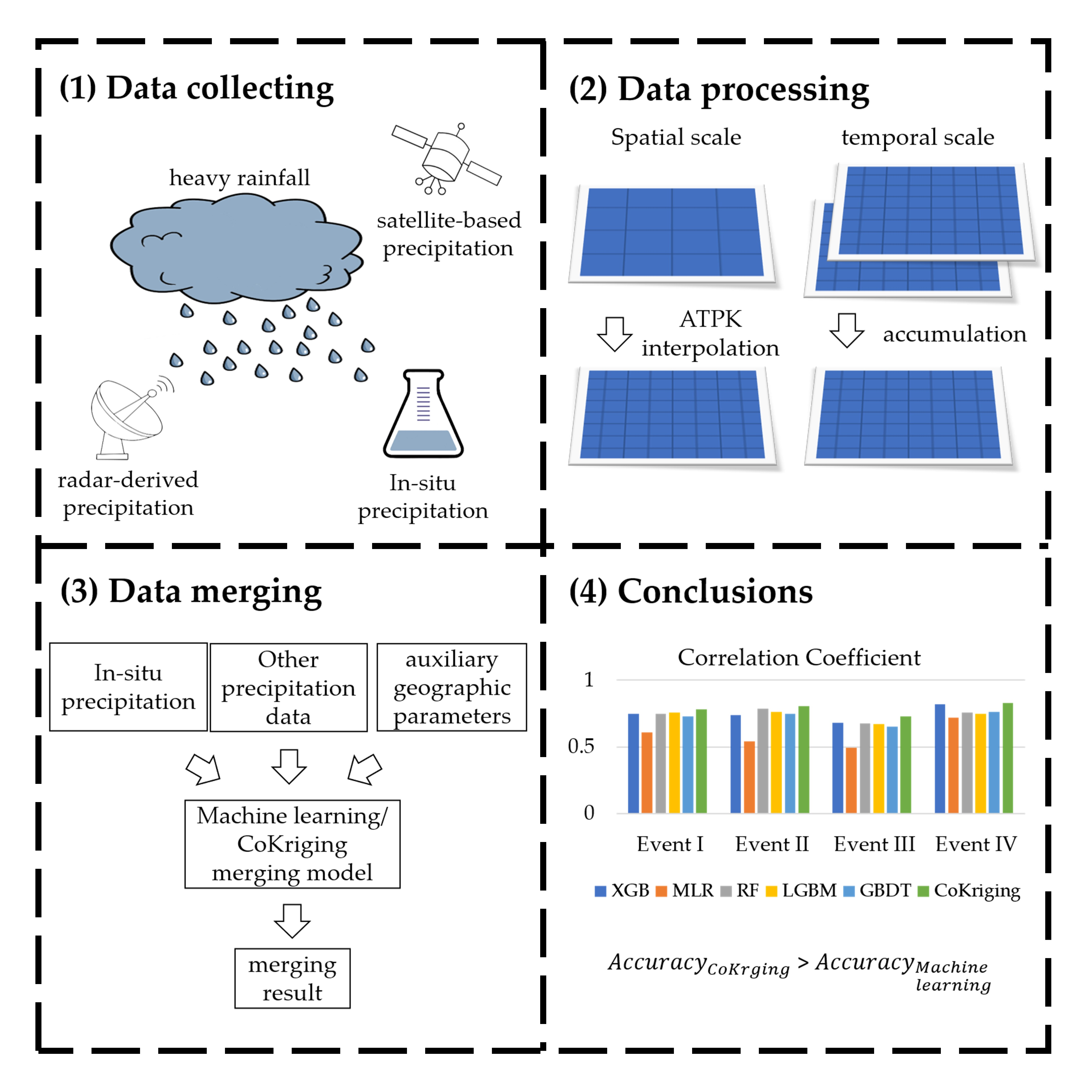
Overview of the Study Area

The study area is located in the mountainous area of Northern Guangdong Province, with a latitude range of 23°33′16″ to 24°33′16″ N and a longitude range of 112°18′2″ to 114°18′38″ E. It includes most areas of Qingyuan City and parts of Zhaoqing, Guangzhou, Huizhou, and Shaoguan, as shown in Figure 1. The eastern and western parts of the study area are mainly composed of mountain ranges, so the overall terrain is high in the east and west and low in the middle, with a maximum elevation difference of 1421 m. The area of lowest elevation is the Beijiang River Valley in Yingde, Qingxin, and Qingcheng in the southeast of Qingyuan, mostly below 20 m. The study area is in a subtropical monsoon climate zone, with an average annual temperature between 18.9 °C and 22 °C. Rainfall is abundant, with an average annual precipitation of 1631.4–2149.3 mm and an annual average of 160–173 days with precipitation (daily precipitation ≥ 0.1 mm/d). The area is located in one of the three belts of heavy rainfall in Guangdong Province and is typical of the parts of Guangdong known as “rain nests” [35]. The heaviest rainfall in the study area is concentrated in Southeastern Qingyuan, Northeastern Guangzhou, Southern Shaoguan, and Northern Huizhou.

2.2. Research Data

Surface topography has a significant effect on precipitation [36]. Therefore, the research data also included auxiliary geographic parameters. Precipitation data were observed at meteorological stations by radar and by satellite; the auxiliary geographic parameters included elevation, distance to the coastline, and latitude and longitude.

2.2.1. Precipitation Data

The station-observed precipitation data used in this study were obtained from the Guangdong Meteorological Bureau (http://data.cma.cn/wa accessed on 1 April 2020). We selected quality-controlled hourly precipitation data, deleting implausible values (data is null or out of reasonable range), obtained from 250 meteorological stations in the study area (Figure 1) for four heavy rainfall events in 2018: event I (monsoon rainstorm, 23 April), event II (monsoon rainstorm, 7–10 May), event III (extreme monsoon rainstorm, 26–30 August), and event IV (Typhoon Mangkhut, 16 and 17 September). Hourly radar-derived precipitation data for the four heavy rainfall events were also used in this study. We used the radar-based quantitative precipitation estimation (RQPE) product provided by the Guangdong Meteorological Bureau, with a spatial resolution of 1 km and a temporal resolution of 6 minutes. First, the reflectivity (Z) during 6-minute volume scans and the corresponding hourly precipitation intensity (I) were used to construct a model of the Z–I relationship, and the 6-minute radar precipitation estimates were inverted; then, the radar data were calibrated by the station data, and the cumulative sum method was used to calculate radar-derived hourly precipitation data with a spatial resolution of 1 km. Satellite precipitation data were obtained from IMERG [37] and GSMaP [38], which use data from GPM mission. GPM is a new-generation global precipitation measurement program, the successor to TRMM and jointly implemented by the National Aeronautics and Space Administration (NASA) and Japan Aerospace Exploration Agency (JAXA) in 2014. Both IMERG and GSMaP are among the most widely used data products currently [39]. This study used IMERG Final Run data with a temporal resolution of half an hour and a spatial resolution of 0.1°. GSMaP precipitation data represent a reanalyzed version of data from the near-real-time Global Rainfall Watch (conducted by JAXA for meteorological and climate research) [40], with a temporal resolution of 1 h and a spatial resolution of 0.1°. GSMaP and IMERG data were downscaled to a spatial resolution of 0.01° and a temporal resolution of 1 h by interpolation using the area-to-point Kriging (ATPK) [41] method and a cumulative summation of the IMERG data.

2.2.2. Auxiliary Geographic Parameters

Elevation was determined based on global digital surface model (DSM) data with a spatial resolution of 30 m, provided by Advanced Land Observing Satellite, Panchromatic Remote-sensing Instrument for Stereo Mapping (ALOS PRISM) (https://www.eorc.jaxa.jp/ALOS/en/aw3d30/index.html accessed on 10 June 2019). ALOS DSM data are produced based on the ALOS panchromatic three-line array imagery (front view, vertical view, and rear view) with a resolution of 2.5 m and global coverage. Their horizontal and vertical accuracy can reach 10 m, and they are widely used to monitor the progress of urban construction and forest growth. By aggregating and averaging the DSM and cropping based on the vector boundaries of study area, a digital elevation model with a spatial resolution of 1 km was obtained.
Data on distance from the coastline were extracted from 2017 Worldview-3 high-resolution remote sensing images through human–computer interactive vectorization. Based on the spatial analysis method, the coordinates of the center point of each 1-km grid in the study area were extracted, and the closest distance from these center points to the coastline was calculated, giving the distance to the coastline of each 1-km grid.

2.3. Methodology

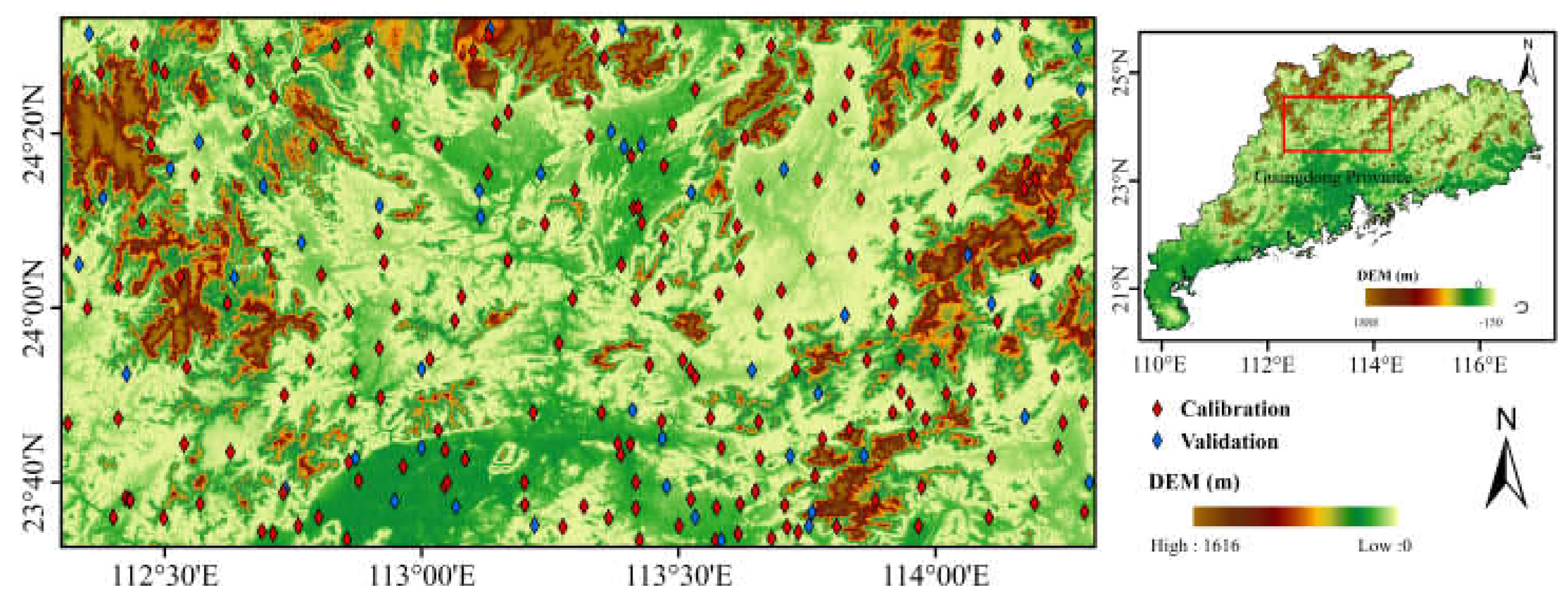
2.3.1. Multi-Source Precipitation Data Merging Methods

We constructed station–radar–satellite hourly precipitation merging models based on machine learning algorithms and geostatistical methods, together with auxiliary geographic parameters, including topography, latitude and longitude, and distance from the coastline. Additionally, to facilitate the high-accuracy merging of multi-source precipitation data, we developed a CoKriging data merging model with station-observed precipitation as the primary variable and the radar precipitation data as a covariate. Finally, merged hourly precipitation data with a spatial resolution of 1 km were obtained. A flowchart of the hourly precipitation data merging methods in this study is shown in Figure 2. There were four main steps: First, IMERG and GSMaP data with a spatial resolution of 0.1° were spatially downscaled using the geostatistical ATPK method, respectively. Second, a regression prediction model was constructed using machine learning algorithms based on the correlation of station precipitation data with radar precipitation data, satellite precipitation data, and auxiliary geographic variables. Third, the residuals between the model estimates and station observations were interpolated using the ordinary Kriging interpolation algorithm. Fourth, the model prediction results were corrected using the interpolated model residuals, producing high-accuracy hourly precipitation merging data with a spatial resolution of 1 km.

2.3.2. Machine Learning-Based Hourly Precipitation Data Merging Models

In this study, five machine learning algorithms (GBDT, XGBoost, LightGBM, RF, and MLR) were used to construct regression models for station precipitation data, radar precipitation data, and auxiliary geographic parameters. The model estimates were compared with CoKriging interpolation results, as shown in Equations (1) and (2). In Equation (1),
P r e c ^ M L = f M L R a d a r ,   I M E R G ,   G s M a P ,   L o n ,   L a t ,   D E M ,   C o a s t l i n e
where P r e c ^ M L denotes precipitation data predicted by a machine learning algorithm; f M L denotes a regression model constructed based on machine learning algorithms; R a d a r , I M E R G , and G s M a P denote radar and satellite precipitation data; L o n and L a t denote latitude and longitude, respectively; D E M denotes elevation; and C o a s t l i n e denotes distance from the coastline. The inputs of the constructed machine learning model were radar precipitation data (spatial resolution of 1 km) and the auxiliary geographic variables, and the output was predicted precipitation data (spatial resolution of 1 km). Then, the residuals of the model were interpolated using the ordinary Kriging interpolation algorithm, as shown in Equation (2):
ε ^ M L x = i = 1 n λ i ε M L X i
where ε ^ M L x is the ordinary Kriging estimate for the residual of the machine learning model at spatial location   x , and λ i denotes the weight of the ordinary Kriging interpolation method. Thus, to obtain high-accuracy precipitation merging data with a spatial resolution of 1 km, it is recommended to use the interpolation results of the model residuals to correct the 1-km precipitation prediction results.

2.3.3. GBDT

The gradient boosting decision tree (GBDT) is an iterative decision tree model, based on a boosting algorithm, that achieves classification and regression by continuously reducing residuals. The GBDT algorithm generates a weak learner with each iteration, and each learner is trained with the residuals of the learner in the previous round until a strong classifier is finally obtained. The core concept of the GBDT algorithm is to let each tree fit the residuals generated by the previous tree and use the cumulative results for all the trees as the final prediction output through formula calculations.

2.3.4. XGBoost

XGBoost is an integrated learning algorithm based on the method of boosting [42]. It is an optimized ensemble tree-based algorithm, improved and extended from the GBDT algorithm. Its main idea is to use feature splitting to grow trees continuously, with each generated tree representing a new function used to fit the residuals of the previous tree; finally, the calculated value of each leaf node is added to obtain the final predictive value:
y ^ i = K = 1 K f k X i ,   f k F
where y ^ i is the model-predicted value, K denotes the number of trees, F is the ensemble space of the regression tree (also known as CART), and X i denotes the feature vector of the i-th data point. F = {   f X = w q X } q : R m T , w R T , where q denotes the structure of each tree by which the examples are mapped to the corresponding leaf indices, T is the number of leaves on the tree, and f k corresponds to the structure q and the leaf weight w of   k -th independent tree. Each regression tree contains consecutive scores on each leaf, and the score on the i -th leaf is denoted by w i . The objective function of the XGBoost algorithm includes a loss function and a regularization term:
L = i l y ^ i , y i + k Ω f k
Ω f = γ T + 1 2 λ | | w | | 2
where l y ^ i , y i denotes the training error between the predicted value y ^ i and true value of the target y i . The regularization term Ω penalizes the complexity of the model to smooth the final learned weight and avoid overfitting, and γ and λ denote the penalty coefficients of the model.

2.3.5. LightGBM

Light Gradient Boosting Machine (LightGBM) is a GBDT variation for big data processing that balances efficiency and accuracy [43]. The characteristics of the LightGBM algorithm are as follows: (1) A leaf-wise algorithm with a depth limit is adopted to replace the level-wise strategy used by most GBDT tools, (2) data volume and accuracy are balanced using a gradient-based one-sided sampling (GOSS) algorithm that can exclude most samples with small gradients and calculate information gain using the remaining samples, and (3) the exclusive feature bundling (EFB) method is used to reduce the data volume by reducing the number of features. LightGBM uses a histogram algorithm to reduce the memory occupied by the method and the complexity of the data separation. Its core idea is to convert continuous features into discrete values and construct a histogram, and the cumulative statistics of each discrete value in the histogram are counted by traversing the training data. During feature selection, the optimal splitting point can be determined by simply traversing the discrete values in the histogram. Moreover, the histogram can be accelerated by the difference. Leaf nodes with large histograms can be obtained based on histogram differences between the small leaf nodes, thus minimizing the computational effort of obtaining histograms for each leaf nodes.

2.3.6. RF

Random forest (RF) is a combination of decision trees where each tree depends on a random vector value with the same distribution as the forest [44]. RF is a product of integrated learning, which combines the integrated Bagging (bootstrap aggregating) [44] and classification and regression tree (CART) algorithms. The idea of RF is to randomly select N samples from the original training sample set repeatedly with replacements to form the sample subsets and then generate N decision trees based on the subsets. Each decision tree is judged to obtain N classification results, and the final classification is determined by voting. RF has the following characteristics: (1) the subsets are independent of each other, which enables parallel computing and ensures high efficiency; (2) because of the Bagging method, the decision tree is not too complex and does not require pruning; and (3) the existence of out-of-bag (oob) data makes it unnecessary to select a validation set separately.

2.3.7. MLR

Based on linear relationships between the precipitation data from meteorological stations, radar precipitation data, and auxiliary geographic parameters, we constructed a multi-source precipitation data merging model based on the multiple linear regression (MLR) method. The parameters of the MLR model were solved by the least squares method to fulfill the requirement that the residual sum of squares Q = i = 1 m P r e c i P r e c ^ i 2 be minimized.

2.4. CoKriging-Based Hourly Precipitation Merging Model

The CoKriging interpolation method interpolates one or more target variables based on several variable data and their spatial and intervariable correlations [45]. In this study, CoKriging interpolation was performed with station-observed precipitation as the primary variable and radar precipitation data as the covariate, as shown in Equation (6):
Z g a u g e , C K * x 0 = i = 1   N 1 λ 1 i Z g a u g e x i + j = 1 N 2 λ 2 j Z r a d a r x j
where   Z g a u g e , C K * x 0 is the estimated value at x 0 ; Z g a u g e x i is the value of the primary variable, station-observed precipitation; Z r a d a r x j is the value of the covariate, the radar precipitation data; λ 1 i and λ 2 j are the weights of Z g a u g e and Z r a d a r , respectively; i = 1   N 1 λ 1 i = 1 ; and j = 1 N 2 λ 2 j = 0 . The CoKriging method uses the variance function and covariance function to perform unbiased optimal estimations according to the following formulae:
γ g a u g e h = 1 2 N h i = 1 N h Z g a u g e x i Z g a u g e x i + h 2
γ g a u g e , r a d a r h = 1 2 N h i = 1 N h Z g a u g e x i Z g a u g e x i + h · Z r a d a r x i Z r a d a r x i + h
where   N ( h ) is the number of samples used to calculate the variance function, and h is the sample distance.

2.5. Evaluation Method

The merging results were evaluated based on precipitation observations from the test stations, and the evaluation indices included the correlation coefficient (CC), root mean square error (RMSE), and mean absolute error (MAE):
C C = i = 1 m P r e c ^ i P r e c ¯ ^ P r e c i P r e c ¯ i = 1 m P r e c ^ i P r e c ¯ ^ 2 i = 1 m P r e c i P r e c ¯ 2
R M S E = 1 m i = 1 m P r e c i P r e c ^ i 2
M A E = 1 m i = 1 m P r e c i P r e c ^ i
where m is the number of stations, P r e c i denotes the precipitation data from the i -th ground-based meteorological station, P r e c ^ i denotes the multi-source precipitation merging data, P r e c ¯ denotes the average station-observed precipitation, and P r e c ¯ ^ denotes the average of the multi-source merging precipitation.

3. Results

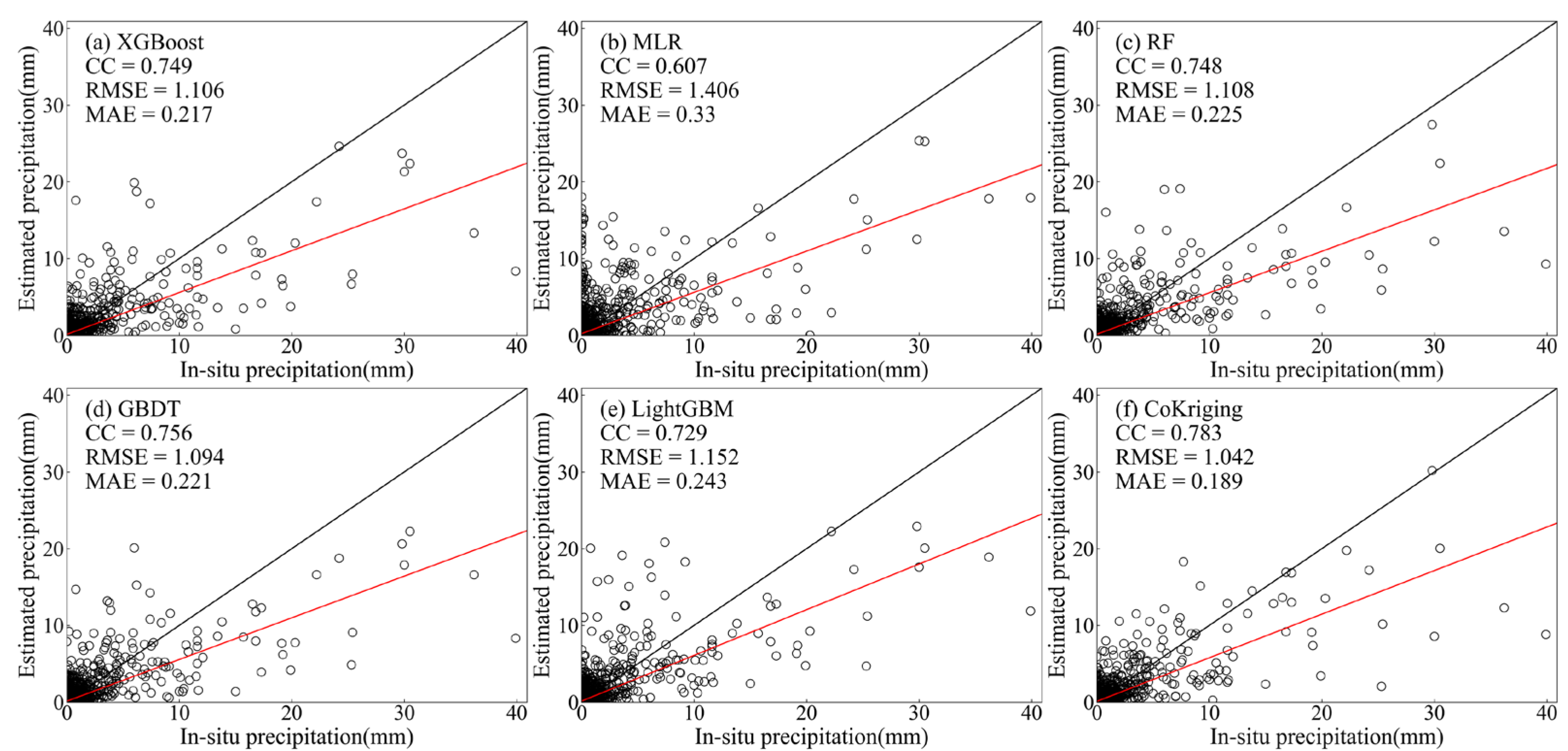
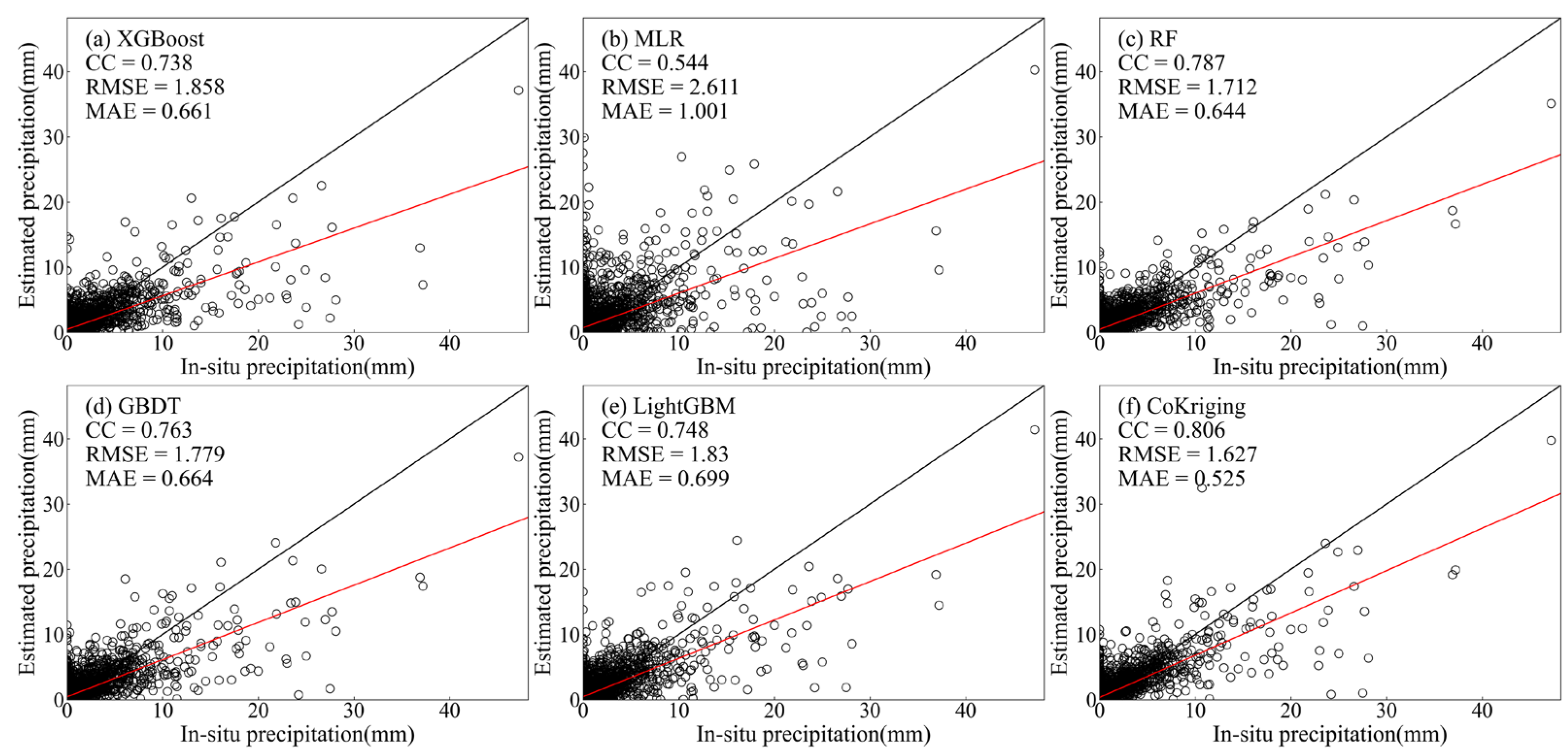
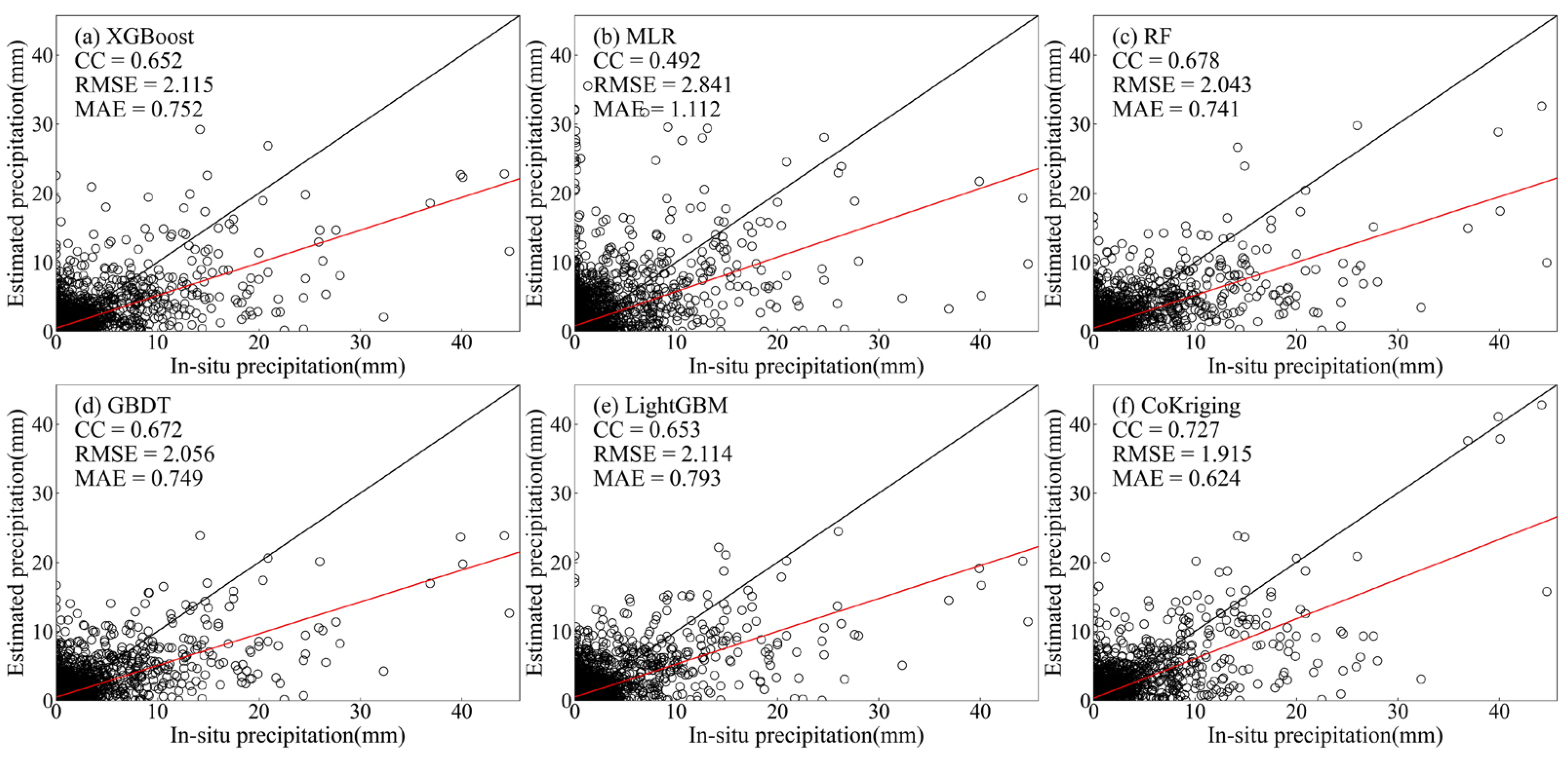
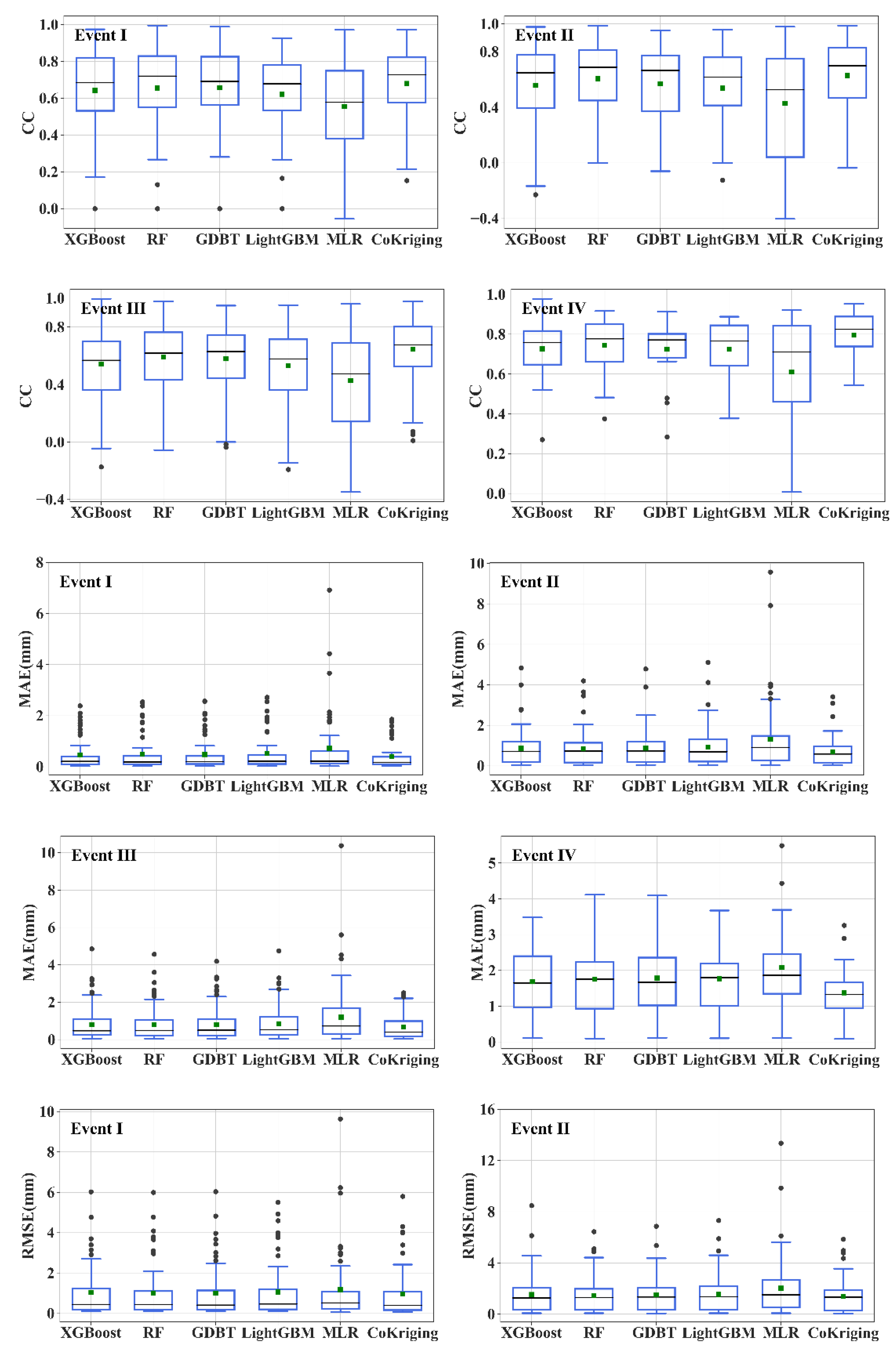
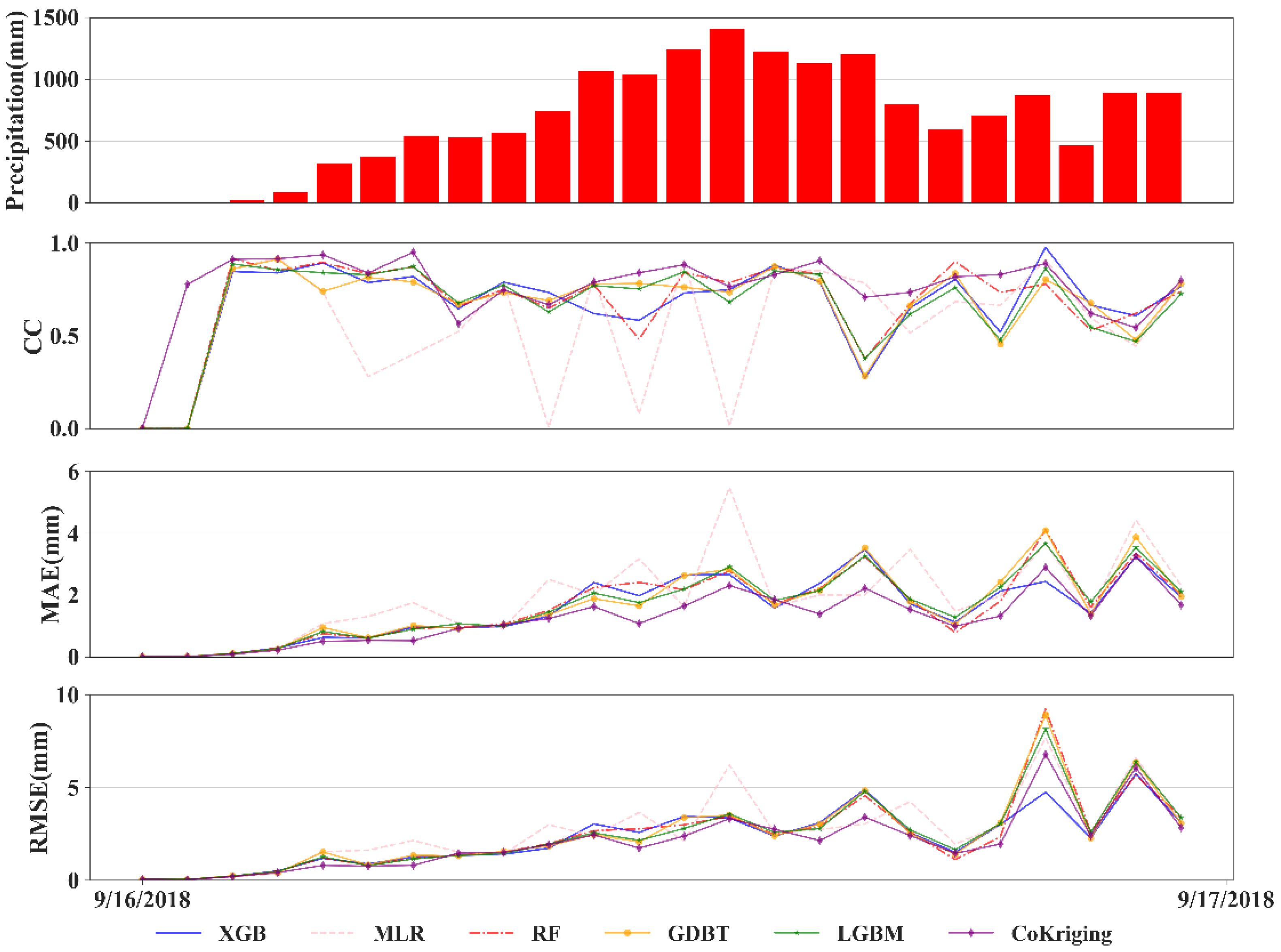
3.1. Evaluation of the Accuracy of Merging Results

Hourly precipitation observations were selected from 20% of the meteorological stations (50 stations), which were evenly distributed over the study area and varied at each timepoint (Figure 1), to evaluate the accuracy of the merged hourly multi-source precipitation data for four heavy rainfall events in terms of the three indices (CC, RMSE, and MAE).
Figure 3, Figure 4, Figure 5 and Figure 6 present the merged precipitation data obtained for the four heavy rainfall events by the six merging methods. The scatterplots show that the main errors were underestimation for high-precipitation timepoints and overestimation for low- or no-precipitation timepoints. CoKriging produced fewer errors in both cases than the machine learning methods, so it was considered the most accurate, giving CC values for the four heavy rainfall events of 0.783, 0.806, 0.727, and 0.828, respectively. Comparing the different machine learning algorithms, GBDT and XGBoost had the best performances for events I (CC = 0.756) and IV (CC = 0.820), respectively, whereas RF provided the highest CC for events II (CC = 0.787) and III (CC = 0.678). MLR resulted in the lowest CC and the highest RMSE and MAE, indicating the lowest accuracy. Moreover, MLR provided the most severe overestimation for the low- and no-precipitation timepoints during events I, II, and III.
Figure 7 shows the boxplots of the evaluation indices for the precipitation timepoints during each heavy rainfall event (when the sum of the observations at the 250 stations was greater than 10 mm). CoKriging produced the highest average and median CC for all four events, as well as the lowest the RMSE and MAE, indicating that CoKriging had the highest merging accuracy. MLR produced the lowest CC distribution and the highest MAE and RMSE. Among the machine learning methods, RF produced the highest upper limit of CC for event I, but its lower limit was still lower than that of CoKriging. For all methods, CC was the lowest for event III compared with the other heavy rainfall events, and the mean CC was below 0.6, except with CoKriging, indicating that the merging performance was worst for event III. The CC values of event IV were generally high, with relatively small variations, and the merging effect was the best, which is because event IV involved high cumulative precipitation, and the rainfall was continuous without abrupt declines (e.g., the periods from 00:00 on 24 April to 23:00 on 25 April, 19:00 on 7 May to 22:00 on 9 May, and 15:00 to 20:00 on 26 August).
Figure 8, Figure 9, Figure 10 and Figure 11 demonstrate the time series of the evaluation indices of the hourly precipitation merging data for the four heavy rainfall events and the sum of the observed hourly precipitation data from all ground-based stations at the corresponding time. It can be seen that CoKriging provides highly accurate hourly precipitation merging data for the four heavy rainfall events, with the CC accounting for over 39%, much higher than that of the five machine learning methods. In addition, the RMSE and MAE of the four heavy rainfall events are highly correlated with the variations of the precipitation values, with basically consistent trends of increases and decreases.
As shown in Figure 8, the accumulated precipitation at the stations for event I started to increase at 12:00 on 23 April and reached the peak of the entire event of about 800 mm at 18:00 on that day. After a pause of two days, the precipitation reached two small peaks at 0:00 on the last two days, respectively; the accuracy of CoKriging for event I was generally higher than that of the other methods. However, there were cases when CoKriging was inferior to other methods. For example, the CC of CoKriging was much lower than that of the other five methods for the timepoint of 23:00 on 26 April. The reasons may be that the precipitation at that timepoint was relatively low and that the rainfall centers were far apart. Thus, the spatial correlation between the precipitation data was relatively weak, making the accuracy of CoKriging lower than that of the machine learning methods. Figure 8 also shows that the CC of MLR was 0 for the timepoint of 18:00 on 23 April when the accumulated precipitation at the stations reached its peak, and the corresponding RMSE and MAE indices were very high. The comparison between MLR merging results plotted in Figure 12 and Figure 13 and the merging results of the other methods revealed that this result was caused by a miscalculation of the precipitation centers with MLR.
As shown in Figure 9, the accumulated precipitation at the stations increased from 100 mm to more than 1500 mm within five hours and then dropped to less than 100 mm in 1 h on the first day of event II. After that, the precipitation continued from 0:00 on 9 May to 10:00 on 10 May, during which it tended to be stable, basically between 200 mm and 600 mm. It could be seen that the CC, RMSE, and MAE of CoKriging were generally better than the other methods for event II. In particular, the accuracy of CoKriging was significantly higher than that of the machine learning methods for the precipitation period from 23:00 on 8 May to 13:00 on 10 May. In addition, for some periods during this heavy rainfall event, the CC of MLR was particularly low, while the RMSE and MAE were notably high.
As shown in Figure 10, event III contained many precipitation peaks with relatively short precipitation intervals, which was quite different from the characteristics of the other monsoon rainstorm events, I and II. For event III, the five machine learning methods all had a CC dominance ratio of about 10%, and CoKriging was still the one with the highest overall accuracy. The advantage of CoKriging was especially pronounced for the period from 0:00 on 26 August to 0:00 on 27 August at the beginning of the heavy rainfall event.
As shown in Figure 11, during event IV, the accumulate precipitation at the stations began to increase from 3:00 on 16 September and peaked at 13:00 on that day. After that, the precipitation continually decreased, showing a normal distribution trend in general. The evaluation indices CC, RMSE, and MAE were still optimal for CoKriging for event IV, yet the ratio of CoKriging dominance decreased compared with the first three heavy rainfall events. In addition, the CC of all the methods except for MLR mostly exceeded 0.5, indicating that the overall merging performance for event IV was better.

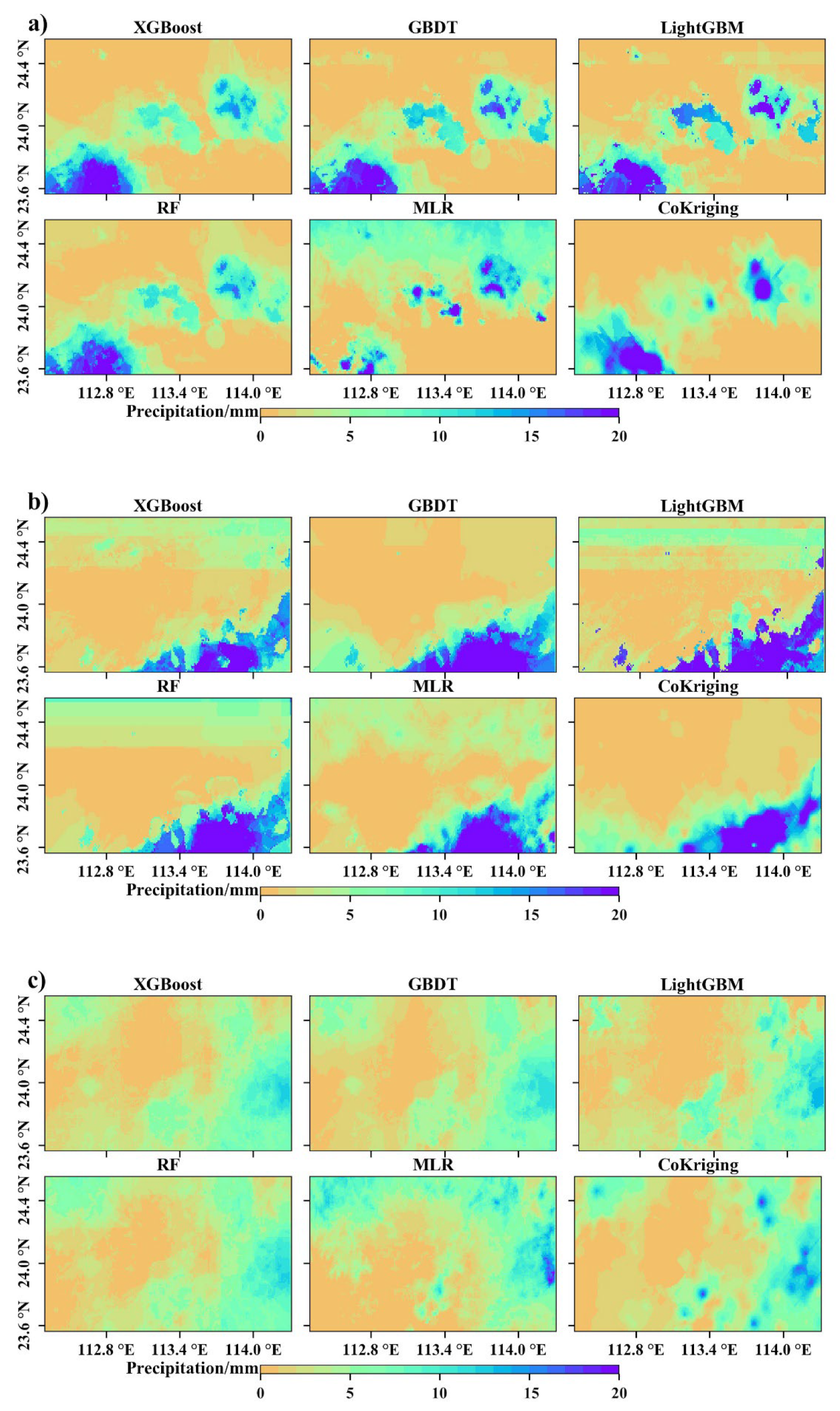
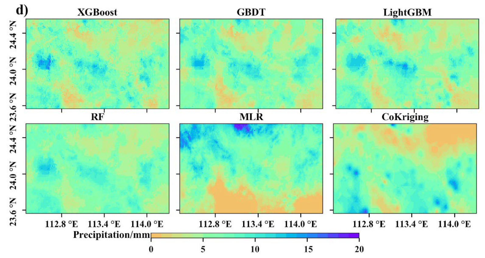
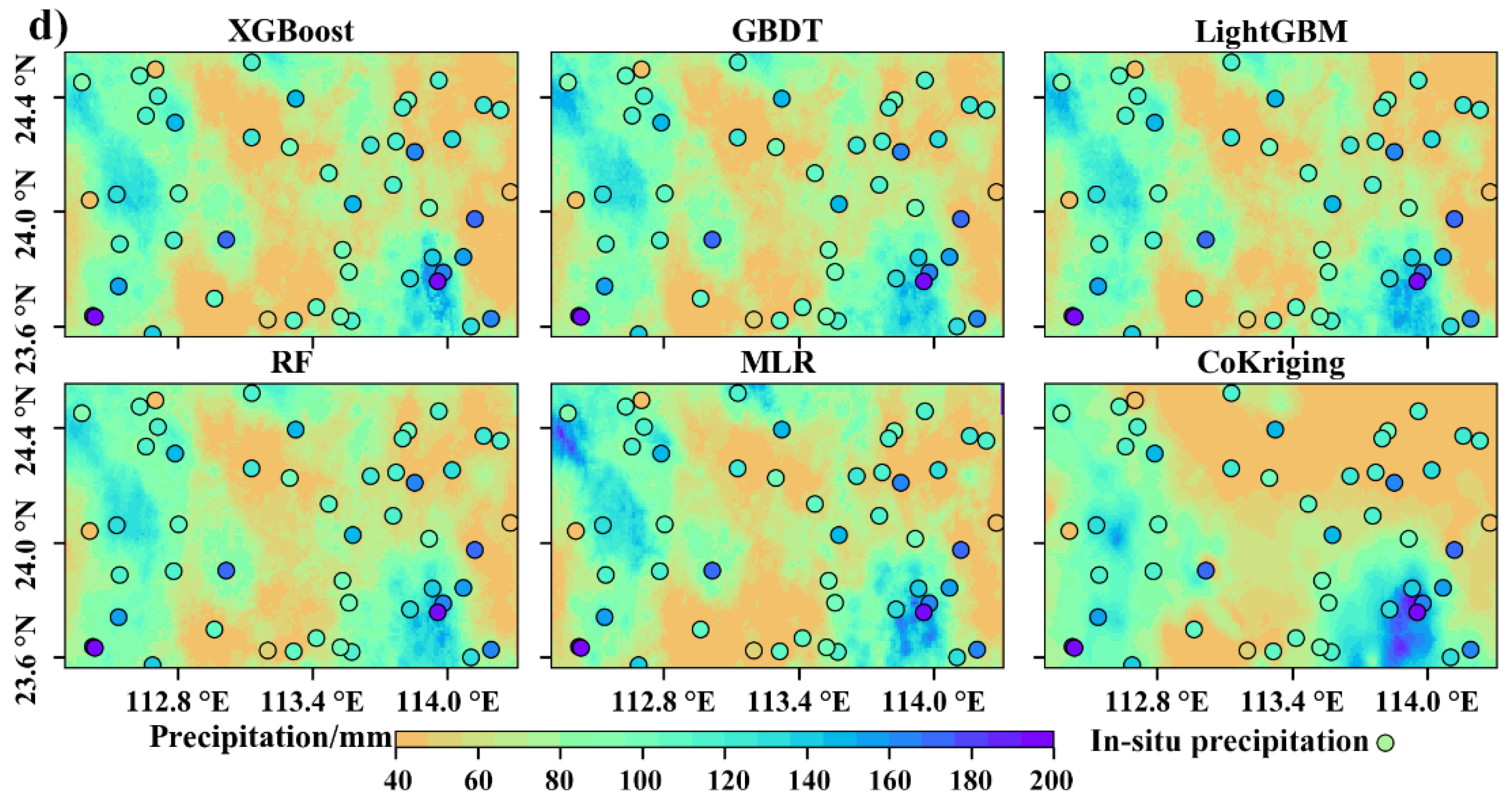
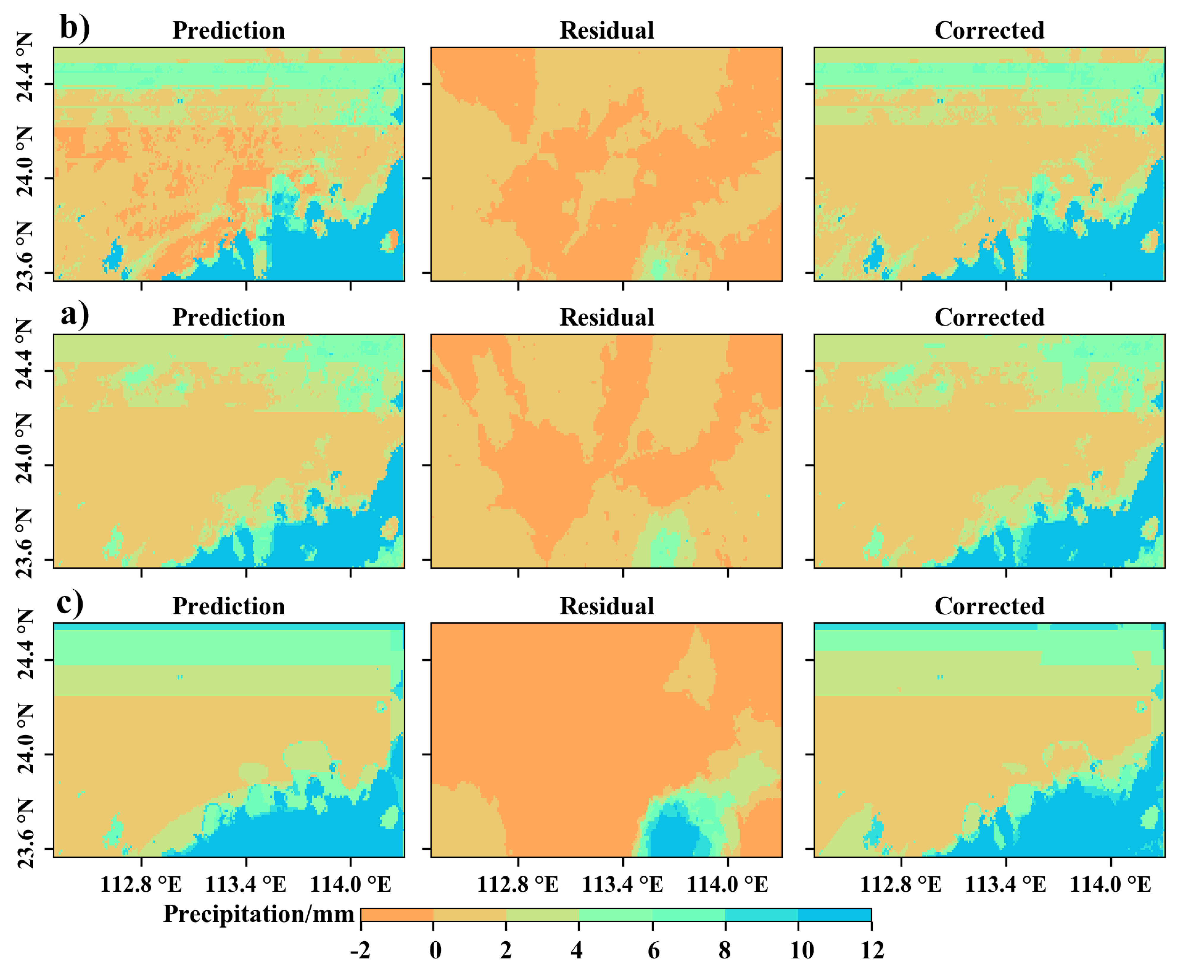
3.2. Merging Result Demonstration

It can be seen from Figure 8, Figure 9, Figure 10 and Figure 11 that the precipitation merging accuracy was not low at timepoints with high observed precipitation during the events, and the precipitation distribution of the peak timepoints was representative. Therefore, Figure 12 demonstrates the merging results of the timepoints with the maximum precipitation in the four heavy rainfall events. Among these, the precipitation was more concentrated at the timepoints of 18:00 on 23 April 2018 and 9:00 on 7 May 2018 than at 7:00 on 30 August 2018 and 13:00 on 16 September 2018 in the merging results. The precipitation distribution of the MLR merging results was significantly different from the results of the other methods at three timepoints: 18:00 on 23 April 2018, 7:00 on 30 August 2018, and 13:00 on 16 September 2018. Referring to the characteristics of the CC, RMSE, and MAE indices of the MLR precipitation merging results at these three timepoints in Figure 8, Figure 9, Figure 10 and Figure 11, we can confirm that MLR miscalculated the precipitation distribution. The reason for this problem was that MLR only considered the linear relationship between the features, and the error was relatively large for some heavy rainfall timepoints. The merging performance of MLR was not as good as the nonlinear machine learning models [46]. The stripes in Figure 12b occur with XGBoost, LightGBM, and RF, and this feature will be discussed in Section 4.3.

4. Discussion

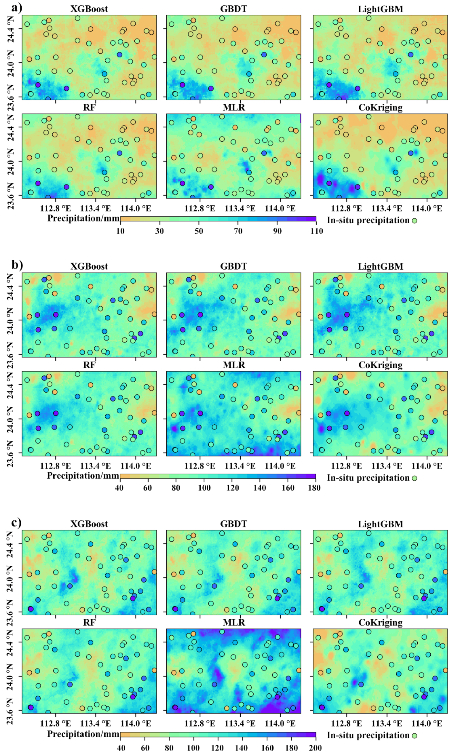
4.1. Spatial Distribution Characteristics of Accumulated Precipitation

Figure 13 shows the spatial distribution of accumulated precipitation obtained by the different merging methods for the four heavy rainfall events in 2018. It can be seen that the accumulated precipitation as determined by the four tree-based machine learning models GBDT, XGBoost, LightGBM, and RF has similar spatial distribution characteristics that are significantly different from those obtained by CoKriging and MLR. Among them, the range of areas with high accumulated precipitation in the results of the RF method is smaller than that for GBDT, XGBoost, and LGBM; the accumulated precipitation results of the XGBoost method are not smooth, with prominent precipitation variations; and the accumulated precipitation results of CoKriging are obviously jagged, which is characteristic of the interpolation method. Finally, the accumulated precipitation results of MLR have a significantly different spatial distribution from the results of the other methods, and the accumulated precipitation values are much higher than the other methods; these are consistent with the hourly prediction results of MLR. The evaluation indices in Figure 3, Figure 4, Figure 5 and Figure 6 and the comparison between the merging results and station-observed precipitation in Figure 13 reveal that the spatial distribution of accumulated precipitation predicted by CoKriging agrees the best with the actual pattern, followed by the results of the tree-based machine learning methods. Furthermore, the distribution characteristics of the accumulated precipitation of the MLR significantly deviate from the actual pattern, showing obvious problems in events II and III.

4.2. Accuracy Analysis

It can be seen from Figure 3, Figure 4, Figure 5 and Figure 6, Figure 7, and Figure 8, Figure 9, Figure 10 and Figure 11 that CoKriging provides the highest CC between the observed and estimated precipitation during the heavy rainfall events, as well as the highest ratio of the timepoints with the best CC performance in the heavy rainfall events, which is sufficient to show that the accuracy of CoKriging is the highest. We believe that there are two main reasons for the high accuracy of the CoKriging merging results. One is that precipitation during the heavy rainfall events has a high spatial autocorrelation, and the other is that CoKriging introduces the highly correlated radar precipitation data as covariate. The dependence on the covariate makes CoKriging less accurate when the correlation between the covariate and station-observed precipitation is relatively low. Among the hourly precipitation merging results for each heavy rainfall event, the CC of MLR is the lowest, and its RMSE and MAE are the highest. The accuracy of MLR is the lowest among the six methods, and its merging results are significantly different from the other methods. The main reason is that MLR only considers the linear relationship of the observed precipitation from the meteorological stations to the radar precipitation data, satellite precipitation data, and auxiliary geographic variables and cannot capture the nonlinear relationship between them, resulting in the miscalculation of the precipitation values and precipitation distribution for some timepoints. For the four heavy rainfall events, the accuracy of each merging method is the lowest for event III, probably because the cumulative value of precipitation from each station in this event is lower than those in events II and IV. In addition, the peak accumulated precipitation is only 1000 mm. There were many timepoints when the accumulated precipitation was relatively little (accumulated precipitation greater than 10 mm and less than 100 mm) during the heavy rainfall event in August, because the little precipitation was only observed by a small number of meteorological stations. The prediction results for such timepoints are poor.
From Figure 8, Figure 9, Figure 10 and Figure 11, it can be seen that the monsoon rainstorms in the mountainous areas of Northern Guangdong Province lasted longer than the typhoon, with more precipitation intervals and more complex temporal precipitation distribution patterns. For the monsoon rainstorm events (events I, II, and III), the machine learning methods with the highest hourly precipitation merging accuracy are GBDT, RF, and RF, respectively, and the merging accuracy of the RF for event I is close to that of GBDT (with CC lower than that of GBDT by 0.007); for the typhoon event (event IV), the machine learning method with the highest merging accuracy is XGBoost, whose merging accuracy is higher than that of LightGBM in second place by 0.06. Therefore, the RF-based hourly precipitation merging model is suitable for analyzing monsoon rainstorm events, and the XGBoost-based hourly precipitation merging model is suitable for analyzing typhoon events.
As can be seen from Figure 12 and Figure 13, the CC of machine learning methods is mostly 0 for the timepoints with little precipitation (from 9:00 on 27 April to 23:00 on 27 April and 20:00 on 7 May to 23:00 on 8 May), while the CC of CoKriging is much higher. This is because the relatively little precipitation was only observed by a small number of meteorological stations. Such cases when few stations observe very little precipitation can only be considered as intermittent precipitation, no longer heavy rainfall. Secondly, it is difficult for the model to extract a precipitation pattern when too few stations have precipitation records. Hence, the model treats such cases as global non-precipitation, but the interpolation results of CoKriging still present some correlation.
Chao [47] used the multiscale geographically weighted regression (MGWR) method to perform hourly precipitation data merging for the Ziwu River Basin, and the CC of the merging result was 0.724. Li [48] applied the space–time multiscale analysis system (STMAS), a multigrid variational analysis technique, to merge hourly precipitation data during the heavy precipitation period in Jiangxi Province from May to June 2019, and the CC of the merging result was 0.76. Figure 3, Figure 4, Figure 5 and Figure 6 show the hourly precipitation merging accuracy of six methods for four heavy rainfall events, where the CC values of the merging results of CoKriging for events I, II, and IV (0.783, 0.806, and 0.828) are higher than the CC of the methods in the two studies mentioned above. The CC of CoKriging for event III (0.726) is also similar to that of GWR and STMAS, and the machine learning methods RF and XGBoost with the highest merging accuracy for events II and IV also provide higher CC results of 0.787 and 0.82. Therefore, the merging results for the four heavy rainfall events in this paper have application and reference values.

4.3. Defects of the Merging Results

There are horizontal stripes in the merging results of the tree-based machine learning methods for some timepoints. Figure 14 shows the merging results of XGBoost, LightGBM, and RF for the rainfall-concentrated timepoint 9:00 on 7 May 2018, where striped areas appear in the regions without concentrated precipitation (the GBDT results do not have stripes at this timepoint, but they are present at other precipitation timepoints). First, the precipitation patterns of these striped areas are obviously inconsistent with the actual precipitation distribution. The correlation coefficients of the observed precipitation from the meteorological stations at 9:00 on 7 May 2018 with the radar precipitation data, GSMaP, IMERG, longitude, latitude, DEM, and distance from the coastline are 0.57, 0.62, 0.62, 0.21, −0.55, −0.15, and −0.62, respectively. It can be seen that the correlation between station-observed precipitation and latitude and distance from the coastline is very high for this timepoint, leading to the overemphasis of XGBoost, LightGBM, and RF on the influence of latitude and distance from the coastline; the striped regions are all high-latitude areas far from the coastline. The striped regions at high latitudes appear under the joint effects of high weights and high eigenvalues. These striped regions do not have particularly large regional residual values, indicating that station-observed precipitation values within the striped regions do not differ significantly from the predicted precipitation values for these regions, but the striped regions cannot be removed simply by residual correction.
Although CoKriging has the highest precipitation merging accuracy, its modeling time is also longer than the machine learning methods. Considering the issues of accuracy and time, we suggest that spatial and temporal autocorrelation parameters should be introduced into machine learning models in further studies and that the influences of ambient precipitation and precipitation at previous timepoints on the modeling results should be fully considered. In addition, the accuracy of the multi-source precipitation data merging model could be improved by incorporating more satellite precipitation data into the model.

5. Conclusions

We selected the mountainous area of Northern Guangdong Province as the study area and used data from four heavy rainfall events during the 2018 flood season (23–27 April, 7–10 May, 26–30 August, and 16 September) to establish precipitation data merging models suitable for the area based on XGBoost, GBDT, LightGBM, RF, MLR, and CoKriging. The residuals of these machine learning models were corrected with the ordinary Kriging method to obtain hourly precipitation merging data with a spatial resolution of 1 km, and the merging results were assessed and analyzed based on the spatial precipitation distribution and accuracy indices. The research conclusions are as follows:
(1)
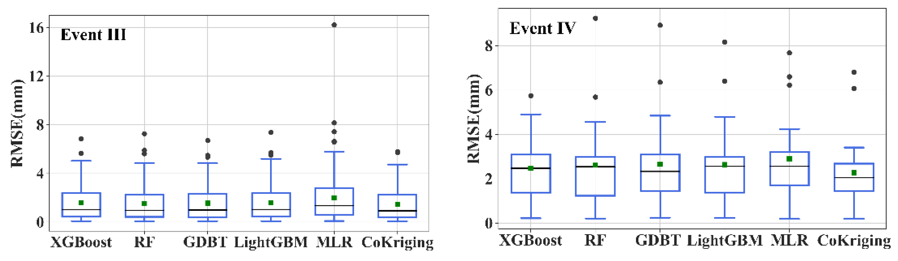
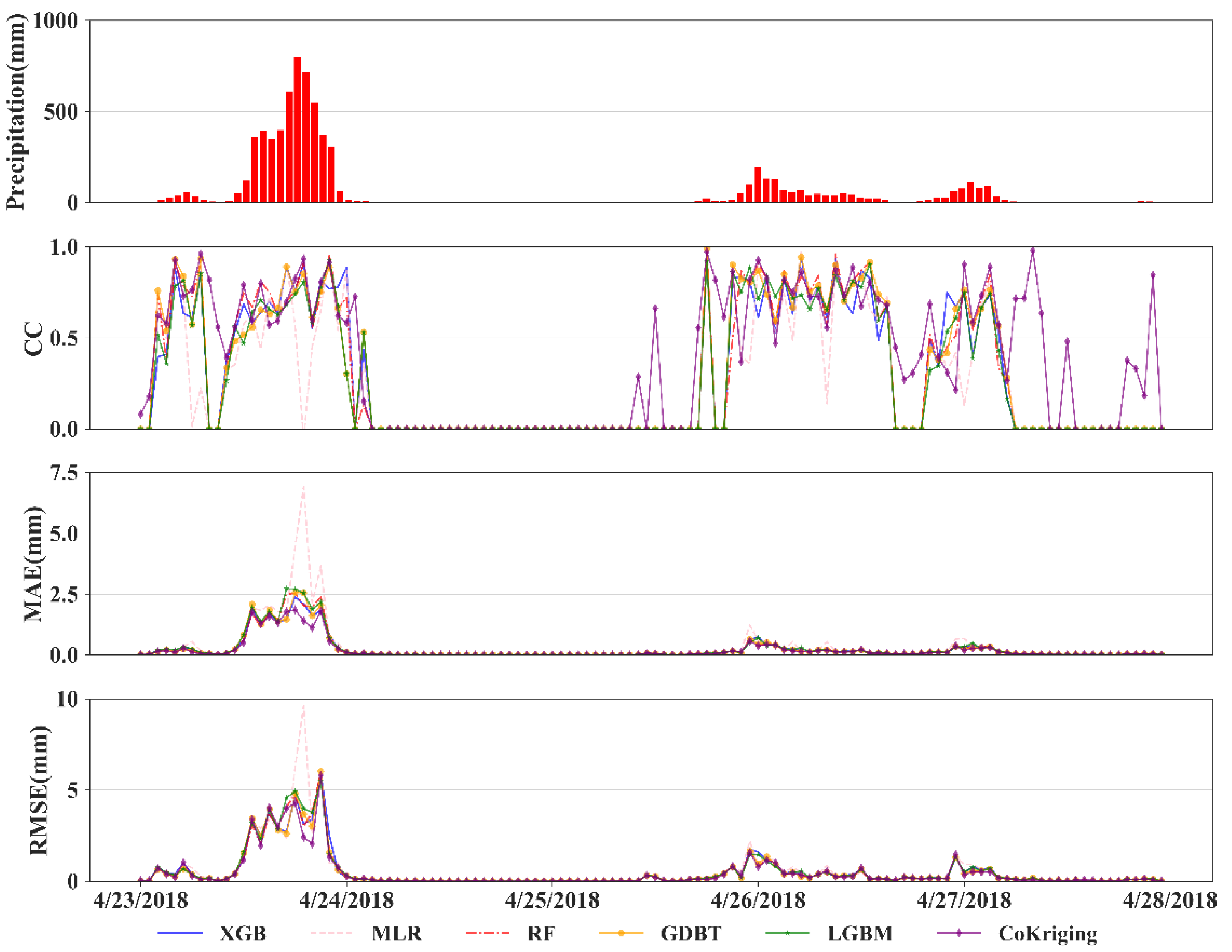
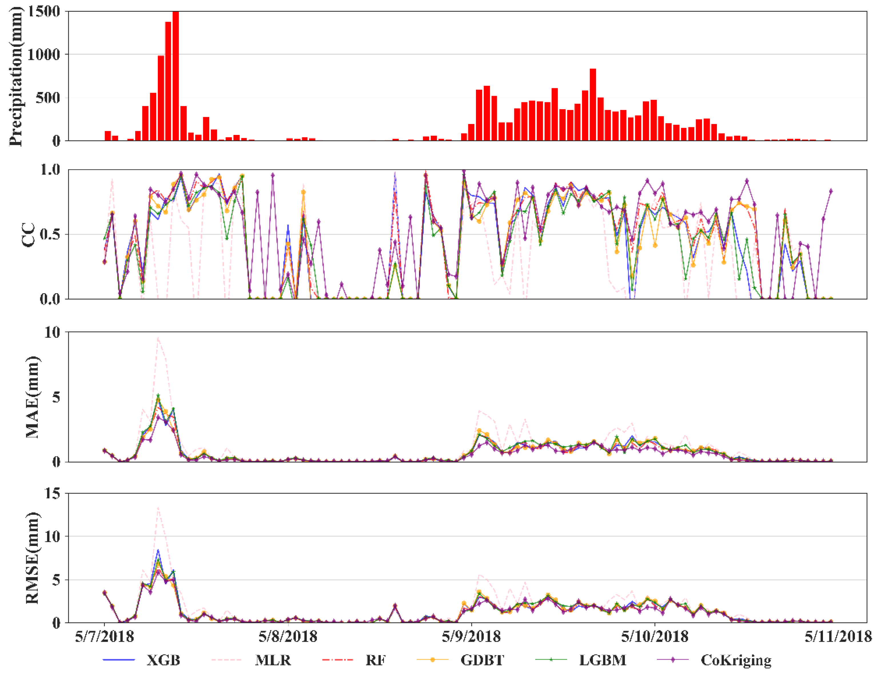
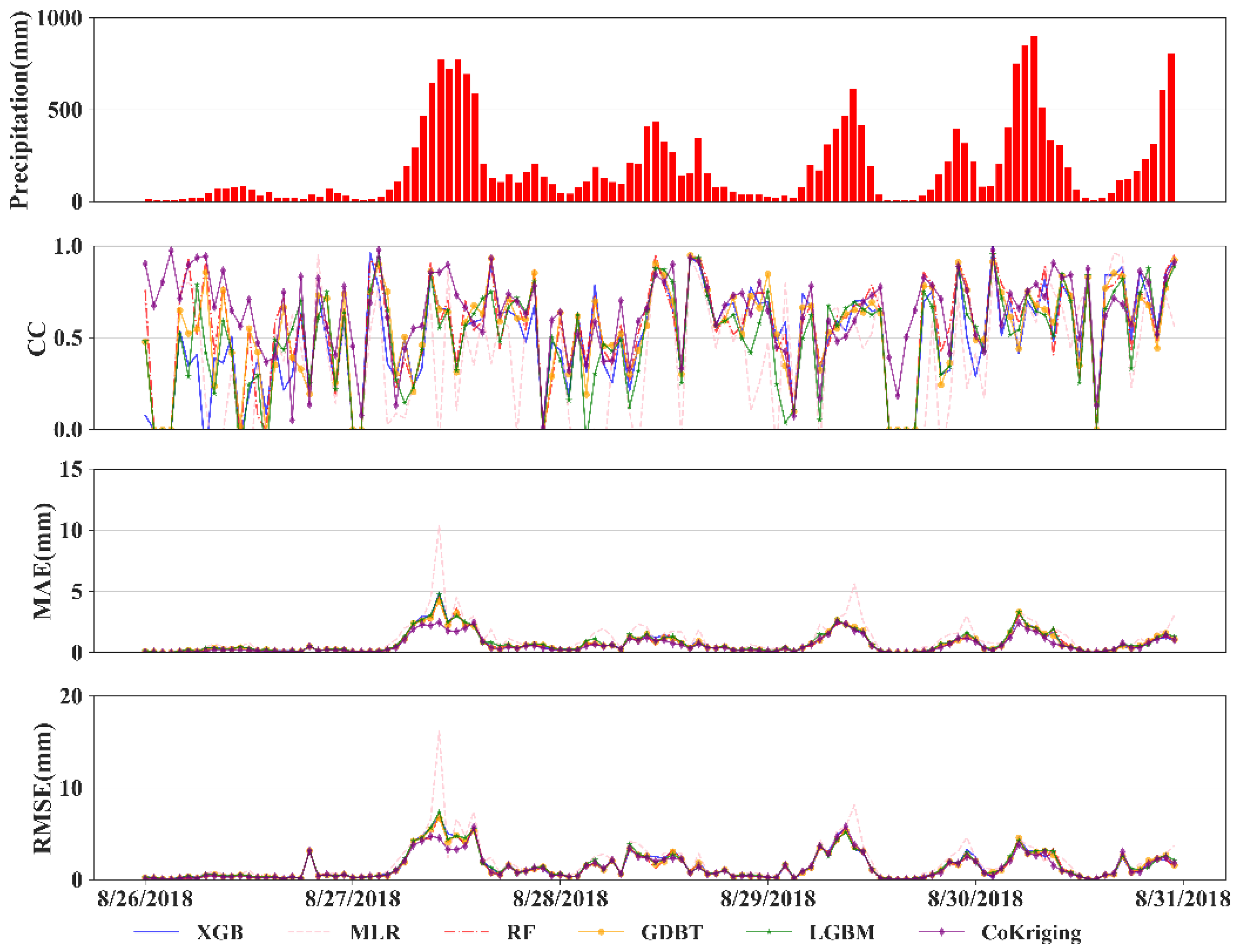
The errors in these precipitation merging results mainly involve underestimations for high-precipitation timepoints and overestimations for low- or no-precipitation timepoints.
(2)
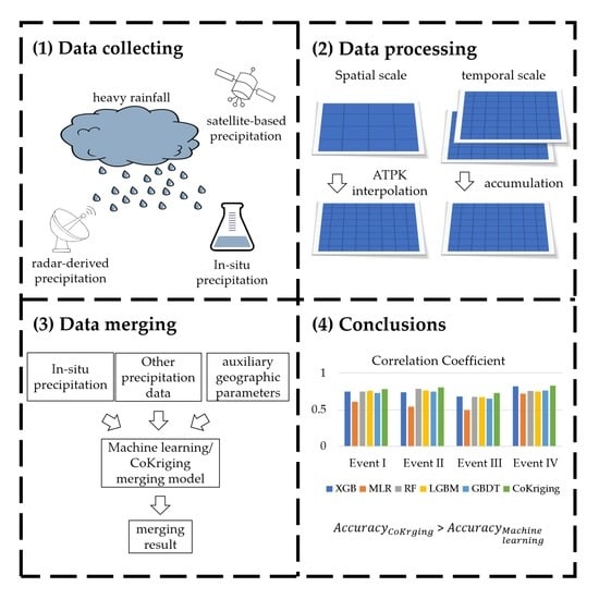
The spatial distribution of the accumulated precipitation predicted by CoKriging agrees the best with the actual pattern, followed by the results of the tree-based machine learning methods, whereas the distribution of accumulated precipitation predicted by MLR is significantly different from the actual pattern. The merging results of CoKriging have a higher accuracy than the machine learning methods, because precipitation during heavy rainfall events has pronounced spatial autocorrelation, and radar precipitation data as a covariate are highly correlated with the station-observed precipitation.
(3)
Different machine learning methods are applicable for different types of heavy rainfall events. The RF-based hourly precipitation merging model is suitable for analyzing monsoon rainstorm events, and the XGBoost-based hourly precipitation merging model is suitable for analyzing typhoon events.
(4)
The merging performance of the machine learning methods is relatively poor for the timepoints, with little precipitation during the heavy rainfall event. One reason is that the models have difficulty in extracting features when a small number of meteorological stations observe little precipitation; another one is the models do not capture the temporal variability of precipitation well, while constant rain is always observed the easiest.
(5)
The hourly merging results of the tree-based machine learning models contain striped textures at some timepoints, which is caused by an excessively high correlation between the precipitation at these timepoints and latitude and distance from the coastline; the MLR method showed miscalculations for the precipitation values and locations and overestimates the accumulated precipitation for heavy rainfall events II, III, and IV.
In summary, the hourly precipitation merging models proposed in this paper can provide high-accuracy gridded precipitation data for heavy rainfall events in the mountainous areas of Northern Guangdong Province. The models combine the advantages of different types of precipitation data by merging precipitation observed from meteorological stations with radar and satellite precipitation data, which is essential for studying different types of heavy rainfall events in mountainous regions. One of their shortcomings is that CoKriging has obvious advantages for the heavy rainfall events in South China, but its applicability in other regions needs further research; the other is that they fail to consider the spatiotemporal autocorrelation of precipitation during heavy rainfall events and that the results for the spatial distribution of precipitation produced by the machine learning methods have certain defects at some timepoints. The models need to be improved in further studies.

Author Contributions

Conceptualization, J.X.; Methodology, J.Z. and J.X.; Software, J.Z.; Validation, J.Z. and H.R.; Formal Analysis, J.Z., J.X. and X.D.; Investigation, J.X. and J.Z.; Resources, H.R. and W.J.; Data Curation, J.X.; Writing—Original Draft Preparation, J.Z.; Writing—Review and Editing, J.X., X.D. and X.L.; Visualization, J.Z.; and Supervision and Project Administration, J.X. All authors have read and agreed to the published version of the manuscript.

Funding

This research was jointly funded by the National Natural Science Foundation of China, grant number 41901371; the Science and Technology Planning Project of Guangdong Province, grant number 2018B020207012; the Key Special Project for Introduced Talents Team of Southern Marine Science and Engineering Guangdong Laboratory (Guangzhou), grant number GML2019ZD0301; the Guangdong Innovative and Entrepreneurial Research Team Program, grant number 2016ZT06D336; the GDAS’ Project of Science and Technology Development, grant number 2019GDASYL-0301001; and the Science and Technology Program of Guangdong, grant number 2021B1212100006.

Institutional Review Board Statement

Not applicable.

Informed Consent Statement

Not applicable.

Data Availability Statement

Not applicable.

Acknowledgments

The authors would like to thank the anonymous reviewers for their constructive comments. We also thank the Geographical Science Data Center of the Greater Bay Area for providing the relevant data in this study.

Conflicts of Interest

The authors declare no conflict of interest.

References

  1. Sapiano, M.; Arkin, P.A. An intercomparison and validation of high-resolution satellite precipitation estimates with 3-hourly gauge data. J. Hydrometeorol. 2009, 10, 149–166. [Google Scholar] [CrossRef]
  2. Taylor, C.M.; de Jeu, R.A.; Guichard, F.; Harris, P.P.; Dorigo, W.A. Afternoon rain more likely over drier soils. Nature 2012, 489, 423–426. [Google Scholar] [CrossRef] [PubMed] [Green Version]
  3. Jieru, Y.; András, B. Short time precipitation estimation using weather radar and surface observations: With rainfall displacement information integrated in a stochastic manner. J. Hydrol. 2019, 574, 672–682. [Google Scholar]
  4. Tapiador, F.J.; Turk, F.J.; Walt, P.; Arthur, Y.H.; Eduardo, G.; Luiz, A.T.M.; Carlos, F.A.; Paola, S.; Chris, K.; George, J.H.; et al. Global precipitation measurement: Methods, datasets and applications. Atmos. Res. 2012, 104, 70–97. [Google Scholar] [CrossRef]
  5. Kidd, C.; Becker, A.; Huffman, G.J.; Muller, C.L.; Joe, P.; Skofronick-Jackson, G.; Kirschbaum, D.B. So, how much of the Earth’s surface is covered by rain gauges? Bull. Am. Meteorol. Soc. 2017, 98, 69–78. [Google Scholar] [CrossRef]
  6. Rana, S.; McGregor, J.; Renwick, J. Precipitation seasonality over the Indian subcontinent: An evaluation of gauge, reanalyses, and satellite retrievals. J. Hydrometeorol. 2015, 16, 631–651. [Google Scholar] [CrossRef]
  7. Xie, P.; Arkin, P.A. Analyses of global monthly precipitation using gauge observations, satellite estimates, and numerical model predictions. J. Clim. 1996, 9, 840–858. [Google Scholar] [CrossRef] [Green Version]
  8. Yilmaz, K.K.; Adler, R.F.; Tian, Y.; Hong, Y.; Pierce, H.F. Evaluation of a satellite-based global flood monitoring system. Int. J. Remote Sens. 2010, 31, 3763–3782. [Google Scholar] [CrossRef]
  9. Arkin, P.A.; Meisner, B.N. The relationship between large-scale convective rainfall and cold cloud over the western hemisphere during 1982-84. Mon. Weather. Rev. 1987, 115, 51–74. [Google Scholar] [CrossRef] [Green Version]
  10. Berg, W.; Chase, R. Determination of mean rainfall from the Special Sensor Microwave/Imager (SSM/I) using a mixed lognormal distribution. J. Atmos. Ocean. Technol. 1992, 9, 129–141. [Google Scholar] [CrossRef] [Green Version]
  11. Xie, P.; Arkin, P.A. Global precipitation: A 17-year monthly analysis based on gauge observations, satellite estimates, and numerical model outputs. Bull. Am. Meteorol. Soc. 1997, 78, 2539–2558. [Google Scholar] [CrossRef]
  12. Huffman, G.J.; Adler, R.F.; Arkin, P.; Chang, A.; Ferraro, R.; Gruber, A.; Janowiak, J.; McNab, A.; Rudolf, B.; Schneider, U. The global precipitation climatology project (GPCP) combined precipitation dataset. Bull. Am. Meteorol. Soc. 1997, 78, 5–20. [Google Scholar] [CrossRef]
  13. Ziqiang, M.; Jintao, X.; Kang, H.; Xiuzhen, H.; Qingwen, J.; TseChun, W.; Wentao, X.; Yang, H. An updated moving window algorithm for hourly-scale satellite precipitation downscaling: A case study in the Southeast Coast of China. J. Hydrol. 2020, 581, 124378. [Google Scholar]
  14. Gao, Y.; Xu, H.; Liu, G. Evaluation of the GSMaP Estimates on Monitoring Extreme Precipitation Events. Remote sensing Technology and Application. Remote Sens. Technol. Appl. 2019, 34, 1121–1132. [Google Scholar]
  15. Michaelides, S.; Levizzani, V.; Anagnostou, E.; Bauer, P.; Kasparis, T.; Lane, J.E. Precipitation: Measurement, remote sensing, climatology and modeling. Atmos. Res. 2009, 94, 512–533. [Google Scholar] [CrossRef]
  16. Zhang, J.; Howard, K.; Langston, C.; Kaney, B.; Qi, Y.; Tang, L.; Grams, H.; Wang, Y.; Cocks, S.; Martinaitis, S. Multi-Radar Multi-Sensor (MRMS) quantitative precipitation estimation: Initial operating capabilities. Bull. Am. Meteorol. Soc. 2016, 97, 621–638. [Google Scholar] [CrossRef]
  17. Shen, Y.; Zhao, P.; Pan, Y.; Yu, J. A high spatiotemporal gauge-satellite merged precipitation analysis over China. J. Geophys. Res. Atmos. 2014, 119, 3063–3075. [Google Scholar] [CrossRef]
  18. Alharbi, R.; Hsu, K.; Sorooshian, S. Bias adjustment of satellite-based precipitation estimation using artificial neural networks-cloud classification system over Saudi Arabia. Arab. J. Geosci. 2018, 11, 1–17. [Google Scholar] [CrossRef] [Green Version]
  19. Xu, G.; Wang, Z.; Xia, T. Mapping Areal Precipitation with Fusion Data by ANN Machine Learning in Sparse Gauged Region. Applied Sciences. 2019, 9, 2294. [Google Scholar] [CrossRef] [Green Version]
  20. Shen, Y.; Pan, S.; Xu, B.; Y, J. Parameter Improvements of Hourly Automatic Weather Stations Precipitation Analysis by Optimal Interpolation over China. J. Chengdu Univ. Technol. 2012, 27, 219–224. [Google Scholar]
  21. Kunwei, L.; Xiong, Y.; Xin, Z.; Fen, T. Multi-source Precipitation Data Fusion Method Based on Filtersim. J. Syst. Simul. 2019, 31, 1232. [Google Scholar]
  22. Wu, H.; Yang, Q.; Liu, J.; Wang, G. A spatiotemporal deep fusion model for merging satellite and gauge precipitation in China. J. Hydrol. 2020, 584, 124664. [Google Scholar] [CrossRef]
  23. Chen, S.; Xiong, L.; Ma, Q.; Kim, J.; Chen, J.; Xu, C. Improving daily spatial precipitation estimates by merging gauge observation with multiple satellite-based precipitation products based on the geographically weighted ridge regression method. J. Hydrol. 2020, 589, 125156. [Google Scholar] [CrossRef]
  24. Delrieu, G.; Wijbrans, A.; Boudevillain, B.; Faure, D.; Bonnifait, L.; Kirstetter, P. Geostatistical radar–raingauge merging: A novel method for the quantification of rain estimation accuracy. Adv. Water Resour. 2014, 71, 110–124. [Google Scholar] [CrossRef]
  25. Sideris, I.V.; Gabella, M.; Sassi, M.; Germann, U. Real-Time Spatiotemporal Merging of Radar and Raingauge Precipitation Measurements in Switzerland. In Proceedings of the 9th International Workshop on Precipitation in Urban Areas, St. Moritz, Switzerland, 6–9 December 2012. [Google Scholar]
  26. Azimi-Zonooz, A.; Krajewski, W.F.; Bowles, D.S.; Seo, D.J. Spatial rainfall estimation by linear and non-linear co-kriging of radar-rainfall and raingage data. Stoch. Hydrol. Hydraul. 1989, 3, 51–67. [Google Scholar] [CrossRef]
  27. Zhang, G.; Tian, G.; Cai, D.; Bai, R.; Tong, J. Merging radar and rain gauge data by using spatial–temporal local weighted linear regression kriging for quantitative precipitation estimation. J. Hydrol. 2021, 601, 126612. [Google Scholar] [CrossRef]
  28. Chen, H.; Chandrasekar, V.; Cifelli, R.; Xie, P. A Machine Learning System for Precipitation Estimation Using Satellite and Ground Radar Network Observations. IEEE Trans. Geosci. Remote 2019, 58, 982–994. [Google Scholar] [CrossRef]
  29. Sønderby, C.K.; Espeholt, L.; Heek, J.; Dehghani, M.; Oliver, A.; Salimans, T.; Agrawal, S.; Hickey, J.; Kalchbrenner, N. Metnet: A neural weather model for precipitation forecasting. arXiv 2020, arXiv:2003.12140. [Google Scholar]
  30. Hazra, A.; Maggioni, V.; Houser, P.; Antil, H.; Noonan, M. A Monte Carlo-based multi-objective optimization approach to merge different precipitation estimates for land surface modeling. J. Hydrol. 2019, 570, 454–462. [Google Scholar] [CrossRef]
  31. Pang, Y.; Shen, Y.; Yu, J.; Xiong, A. An experiment of high-resolution gauge-radar-satellite combined precipitation retrieval based on the Bayesian merging method. Acta Meteorol. Sin. 2015, 73, 177–186. [Google Scholar]
  32. Wehbe, Y.; Temimi, M.; Adler, R.F. Enhancing precipitation estimates through the fusion of weather radar, satellite retrievals, and surface parameters. Remote Sens.-Basel 2020, 12, 1342. [Google Scholar] [CrossRef] [Green Version]
  33. Li, J.; Yu, R.; Sun, W. Duration and seasonality of the hourly extreme rainfall in the central-eastern part of China. Acta Meteorol. Sin. 2013, 71, 652–659. [Google Scholar]
  34. Trenberth, K.E.; Dai, A.; Rasmussen, R.M.; Parsons, D.B. The changing character of precipitation. Bull. Am. Meteorol. Soc. 2003, 84, 1205–1218. [Google Scholar] [CrossRef]
  35. Li, D.; Chen, W.; Ye, A. Climatic characteristics and forecast focus of heavy rain in Qingyuan. Guangdong Meteorol. 1999, 2, 8–10. [Google Scholar]
  36. Roe, G.H. Orographic precipitation. Annu. Rev. Earth Planet. Sci. 2005, 33, 645–671. [Google Scholar] [CrossRef]
  37. Huffman, G.J.; Bolvin, D.T.; Braithwaite, D.; Hsu, K.; Joyce, R.; Xie, P.; Yoo, S. NASA global precipitation measurement (GPM) integrated multi-satellite retrievals for GPM (IMERG). Algorithm Theor. Basis Doc. ATBD Version 2015, 4, 26. [Google Scholar]
  38. Shige, S.; Yamamoto, T.; Tsukiyama, T.; Kida, S.; Ashiwake, H.; Kubota, T.; Seto, S.; Aonashi, K.; Okamoto, K. The GSMaP precipitation retrieval algorithm for microwave sounders—Part I: Over-ocean algorithm. IEEE Trans. Geosci. Remote 2009, 47, 3084–3097. [Google Scholar] [CrossRef]
  39. Hou, A.Y.; Kakar, R.K.; Neeck, S.; Azarbarzin, A.A.; Kummerow, C.D.; Kojima, M.; Oki, R.; Nakamura, K.; Iguchi, T. The global precipitation measurement mission. Bull. Am. Meteorol. Soc. 2014, 95, 701–722. [Google Scholar] [CrossRef]
  40. Ushio, T.; Sasashige, K.; Kubota, T.; Shige, S.; Okamoto, K.; Aonashi, K.; Inoue, T.; Takahashi, N.; Iguchi, T.; Kachi, M. A Kalman filter approach to the Global Satellite Mapping of Precipitation (GSMaP) from combined passive microwave and infrared radiometric data. J. Meteorol. Soc. Jpn. Ser. II. 2009, 87, 137–151. [Google Scholar] [CrossRef] [Green Version]
  41. Kyriakidis, P.C. A geostatistical framework for area-to-point spatial interpolation. Geogr. Anal. 2004, 36, 259–289. [Google Scholar] [CrossRef]
  42. Chen, T.; Guestrin, C. Xgboost: A Scalable Tree Boosting System. In Proceedings of the 22nd ACM SIGKDD International Conference on Knowledge Discovery and Data Mining, San Francisco, CA, USA, 13–17 August 2016; pp. 785–794. [Google Scholar]
  43. Ke, G.; Meng, Q.; Finley, T.; Wang, T.; Chen, W.; Ma, W.; Ye, Q.; Liu, T. Lightgbm: A highly efficient gradient boosting decision tree. Adv. Neural Inf. Processing Syst. 2017, 30, 3146–3154. [Google Scholar]
  44. Breiman, L. Bagging predictors. Mach. Learn. 1996, 24, 123–140. [Google Scholar] [CrossRef] [Green Version]
  45. Zhang, R. Spatial Variation Theory and Applications; Science Press: Beijing, China, 2005. [Google Scholar]
  46. Huang, X.; He, L.; Zhao, H.; Huang, Y.; Wu, Y. Prediction model based on the Laplacian eigenmap method combined with a random forest algorithm for rainstorm satellite images during the first annual rainy season in South China. Nat. Hazards 2021, 107, 331–353. [Google Scholar] [CrossRef]
  47. Chao, L.; Zhang, K.; Li, Z.; Zhu, Y.; Wang, J.; Yu, Z. Geographically weighted regression based methods for merging satellite and gauge precipitation. J. Hydrol. 2018, 558, 275–289. [Google Scholar] [CrossRef]
  48. Li, X.; Wei, Z.; Shaoping, H.; Weihua, D.; Xueying, Z. Analysis of fusion test results on hourly precipitation from meteorological and hydrological stations and radar. Torrential Rain Disasters 2020, 39, 276–284. [Google Scholar]
Figure 1. Study area and the distribution of the meteorological stations.
Remotesensing 14 01750 g001
Figure 2. Flow chart of multi-source precipitation data merging.
Remotesensing 14 01750 g002
Figure 3. Comparison of the observed and estimated precipitation for heavy rainfall event I: (a) XGBoost, (b) MLR, (c) RF, (d) GBDT, (e) LightGBM, (f) CoKriging (the red line represents the fitted curve between in-situ and estimated precipitation; the black line represents that the ratio of in-situ precipitation to estimate precipitation is 1:1).
Remotesensing 14 01750 g003
Figure 4. Comparison of the observed and estimated precipitation for heavy rainfall event II: (a) XGBoost, (b) MLR, (c) RF, (d) GBDT, (e) LightGBM, (f) CoKriging (the red line represents the fitted curve between in-situ and estimated precipitation; the black line represents that the ratio of in-situ precipitation to estimate precipitation is 1:1).
Remotesensing 14 01750 g004
Figure 5. Comparison of the observed and estimated precipitation for heavy rainfall event III: (a) XGBoost, (b) MLR, (c) RF, (d) GBDT, (e) LightGBM, (f) CoKriging (the red line represents the fitted curve between in-situ and estimated precipitation; the black line represents that the ratio of in-situ precipitation to estimate precipitation is 1:1).
Remotesensing 14 01750 g005
Figure 6. Comparison of the observed and estimated precipitation for heavy rainfall event IV: (a) XGBoost, (b) MLR, (c) RF, (d) GBDT, (e) LightGBM, (f) CoKriging (the red line represents the fitted curve between in-situ and estimated precipitation; the black line represents that the ratio of in-situ precipitation to estimate precipitation is 1:1).
Remotesensing 14 01750 g006
Figure 7. Boxplots of the evaluation indices for the four heavy rainfall events: event I, 23–27 April; event II, 7–10 May; event III, 26–30 August; and event IV, 16 and 17 September.
Remotesensing 14 01750 g007aRemotesensing 14 01750 g007b
Figure 8. Evaluation indices of heavy rainfall event I.
Remotesensing 14 01750 g008
Figure 9. Evaluation indices of heavy rainfall event II.
Remotesensing 14 01750 g009
Figure 10. Evaluation indices of heavy rainfall event III.
Remotesensing 14 01750 g010
Figure 11. Evaluation indices of heavy rainfall event IV.
Remotesensing 14 01750 g011
Figure 12. Distribution of the merging results based on the XGBoost, GBDT, LightGBM, RF, and MLR algorithms and the CoKriging interpolation results: (a) 18:00 on 23 April 2018, (b) 9:00 on 7 May 2018, (c) 7:00 on 30 August 2018, and (d) 13:00 on 16 September 2018.
Remotesensing 14 01750 g012aRemotesensing 14 01750 g012b
Figure 13. Spatial distribution of the accumulated precipitation merging results of different merging methods for the four heavy rainfall events: (a) heavy rainfall event I, (b) heavy rainfall event II, (c) heavy rainfall event III, and (d) heavy rainfall event IV.
Remotesensing 14 01750 g013aRemotesensing 14 01750 g013b
Figure 14. Residual correction for the results of the XGBoost, LightGBM, and RF methods at 9:00 on 7 May 2018: (a) XGBoost, (b) LightGBM, and (c) RF.
Remotesensing 14 01750 g014
Publisher’s Note: MDPI stays neutral with regard to jurisdictional claims in published maps and institutional affiliations.

