Machine Learning for Defining the Probability of Sentinel-1 Based Deformation Trend Changes Occurrence

Abstract

The continuous monitoring of displacements occurring on the Earth surface by exploiting MTInSAR (Multi Temporal Interferometry SAR) Sentinel-1 data is a solid reality, as testified by the ongoing operational ground motion service in the Tuscany region (Central Italy). In this framework, anomalies of movement, i.e., accelerations or deceleration as seen by the time series of displacement of radar targets, are identified. In this work, a Machine Learning algorithm such as the Random Forest has been used to assess the probability of occurrence of the anomalies induced by slope instability and subsidence. About 20,000 anomalies (about 7000 and 13,000 for the slope instability and the subsidence, respectively) were collected between 2018 and 2020 and were used as input, while ten different variables were selected, five related to the morphological and geological setting of the study area and five to the radar characteristics of the data. The resulting maps may provide useful indications of where a sudden change of displacement trend may occur, analyzing the contribution of each factor. The cross-validation with the anomalies collected in a following timespan (2020–2021) and with official landslide and subsidence inventories provided by the regional authority has confirmed the reliability of the final maps. The adoption of a map for assessing the probability of the occurrence of MTInSAR anomalies may serve as an enhanced geohazard prevention measurement, to be periodically updated and refined in order to have the most precise knowledge possible of the territory.

1. Introduction

The detection and mapping of geological hazards are paramount activities for land management and risk reduction policies. Indeed, geohazards can result in the loss of human lives, extensive physical damage to buildings and critical infrastructure. According to the Emergency Events Database (https://public.emdat.be/, accessed on 18 February 2022), in 2021 about 250 geohazards have occurred worldwide, claiming the lives of more than 150 people and affecting almost 20 million people in total, while Franceschini, et al. [1] found that over 13,000 landslide events were reported in Italy from 2010 to 2019, with more than 300 of these in the Tuscany region. Ground motion events, such as landslides and subsidence, can be easily monitored by a wide spectrum of techniques, depending on the scale of analysis and the intensity of the deformation. Earth observation spaceborne practices, and especially InSAR and MTInSAR methods (Interferometry Synthetic Aperture Radar and Multi-Temporal InSAR), have demonstrated their suitability for a wide range of slow-moving ground motion phenomena and the variety of scale of analysis, i.e., continental [2,3], national [4,5,6,7], regional [8,9,10,11,12,13] and very local [14,15,16,17,18], performing very well either for the monitoring and analysis of subsidence [19,20] or landslides [21,22,23]. The present abundance of SAR imagery, the simultaneous activity of many SAR systems and the shortening of the revisit time, in particular with the launch of the Sentinel-1 (S-1) constellation (six days with the dual system), along with the improvement of very precise and fast delivering processing techniques, such as the SqueeSAR [24] and the P-SBAS [25], enabled the development of continuous monitoring services relying on spaceborne InSAR data. Indeed, the Tuscany Region, followed by Valle d’Aosta and Veneto (Central, NW and NE Italy, respectively), started an operational service based exclusively on S-1 data, that benefitted from regularly updated deformation maps (every 12 days) and identified the so-called anomalies of deformation, i.e., trend variations in the time series of displacement. This service is implemented as a tool to support the regional authorities in charge of the geological risks. More detail of the procedure can be found in Raspini, et al. [26], Del Soldato, et al. [27] and in Confuorto, et al. [28], who provided critical analysis of the distribution of the anomalies collected in the three regions. However, the monitoring systems both detect and follow a certain displacement event, without having the ability to estimate the propensity of a territory to be affected by deformation or an acceleration of movements.

In this work, an assessment of the Probability of Occurrence (PO) of the MTInSAR anomalies is provided, through the use of a Machine Learning (ML) algorithm in order to analyze the main factors, which lead to changes in the deformation trends. The expression PO is used here to distinguish this concept from the classical susceptibility, referred to as the spatial occurrence of natural hazards such as landslides. The use of ML approaches has widely demonstrated their suitability in many scientific fields, including landslide susceptibility modeling, since they are characterized by high accuracy and specific advantages in different study areas and for different sets of factors [29,30]. Many ML methods have been widely implemented for the generation of susceptibility maps [31], such as Random Forest [32], Support Vector Machine [33], Artificial Neural Network [34,35] or MaxEnt [36,37] and many others. Several works have jointly used InSAR data and ML models, such as InSAR data to map subsiding areas, and ML for modeling the susceptibility to subsidence [38,39,40] or landslides [41,42,43]. However, no standard methodology to assess the probability of areas to experience a change in deformation trends, highlighted by InSAR technologies, has ever been established. In this work, the Random Forest [44], based on classification trees, was adopted. This approach was already implemented for the classification of remote sensing data [45] and landslide susceptibility evaluation [32,46,47,48]. This study aims to assess the areas most likely to detect displacement trend anomalies, according to several characteristics, either of the territory or of the radar system. The Tuscany Region was selected as study area as it was the first to embrace the monitoring system and therefore had a robust database of anomalies. Four different spatial probability maps were generated; two related to Slope Instabilities (SI), one for the ascending, and one for descending geometry, and two to Subsidence (S) anomalies, one for each orbit. To create them, ten environmental variables were selected; five connected to the radar data, and five to the morphology and geology of the study area. Finally, ascending and descending anomalies Probability of Occurrence (PO) maps were merged to have a single final map of the PO of SI and S anomaly events.

The resulting maps may provide useful indications of where a sudden change in displacement trends may occur, according to the characteristic of the territory and of the radar data by MTInSAR data. This information could be a valuable support for the territory screening activities by the regional authorities, in order to have an evaluation of the areas potentially affected by accelerating displacement events. Moreover, the methodology can be also implemented at a national scale, as the used data is easily accessible.

2. Materials and Methods

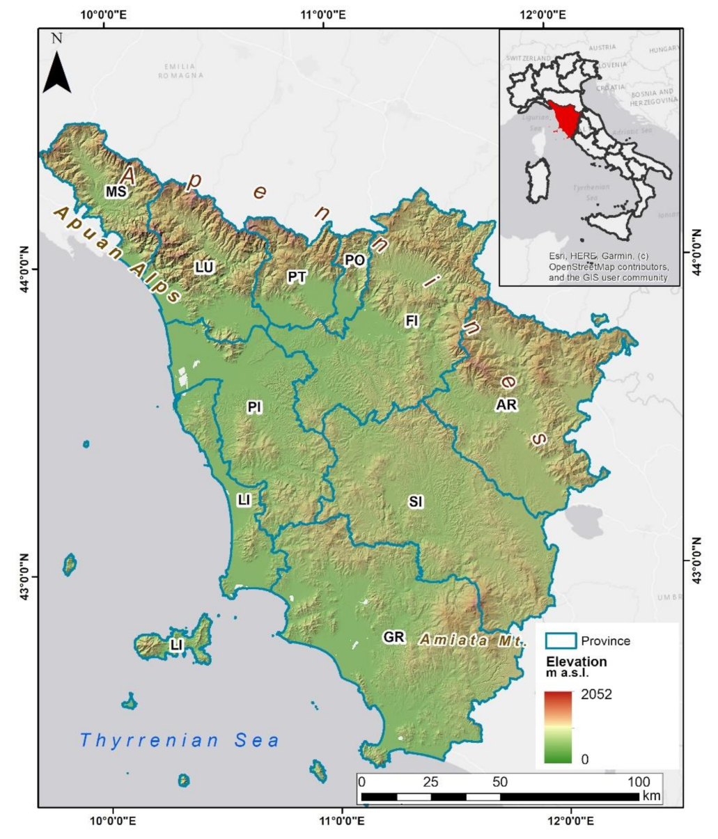
2.1. Tuscany Region

Tuscany is one of the biggest regions in Italy, covering almost 23,000 km² in the central part of the country, between the Emilia–Romagna, Umbria, Marche, and Lazio regions, and extending along the Tyrrhenian coast (Figure 1). The Tuscany region includes the Tuscan Archipelago, formed by seven islands, with Elba and Giglio islands being the largest ones. The geomorphological setting of Tuscany is extremely variegated, presenting wide plains, along the coast, such as in the area of Grosseto (SW) or Pisa (NW), and the main rivers (the Firenze–Prato–Pistoia plain, along the Arno river, in the Northern part, and Val di Chiana, between the Siena and Arezzo provinces, in the SE sector), hilly areas, in the central sector embracing all the provinces and counting for more than 60% of the territory, and, along the E flank, the mountainous sector represented by the Apennine ridge, running from NW to SE and reaching heights greater than 2000 m a.s.l. The morphology of the territory in Tuscany is a clear reflection of the tectonic history of the area. Indeed, the Northern Apennine consists of a NE-oriented fold-and-thrust belt, that originated during the Cretaceous [49]. The Apennines Mountain range is the result of the overlap of three main geological units: the Ligurian, the Tuscan and the Umbro–Marchigian units [50,51]. The Ligurian units are made from the remains of the oceanic crust and their sedimentary cover; the Tuscan domain is basically composed of two units, the metamorphic and the non-metamorphic units; the Umbro–Tuscan unit consists of a thick sedimentary sequence of carbonate and silicoclastic deposits. The geomorphological and geological settings, combined with the variety of climatic seasons, make the Tuscan territory prone to ground deformational phenomena: different types of landslides can be experienced, according to the lithology and the morphology [52,53], as well as plain areas being, at times, affected by subsidence, such as the Florence–Prato–Pistoia and Chiana plains, mostly due to water over-exploitation, and the Larderello geothermal site [54,55,56,57].

2.2. Input Data

The data used for the application of the Random Forest (RF) model can be split into two groups: the anomalies inventory; and the environmental and radar variables used as predisposing factors (PF). The flowchart in Figure 2 summarizes the use of the input data within the implemented model and provides a conceptual model of the work carried out.

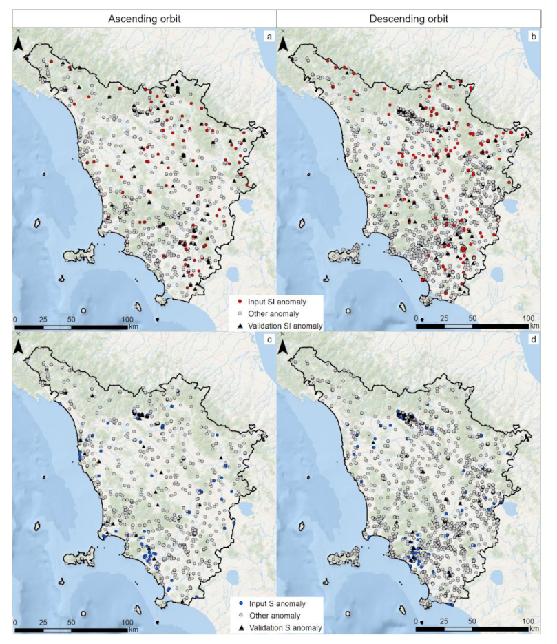
2.2.1. Anomalies Inventory

The regional continuous monitoring services benefit from Sentinel-1 (both A and B) data. The initial analysis was conducted by acquiring and processing, through the usage of SqueeSAR technique [24], a second-generation PSInSAR algorithm capable of processing long temporal stacks of SAR images, and, acquired over the same area, the entire ESA images archive of Sentinel-1 imagery. Unlike the PSInSAR approach, however, the SqueeSAR technique allows one to measure displacements by exploiting both point-wise coherent scatterers (i.e., the Persistent Scatterers, PS) and partially coherent Distributed Scatterers (DS). The basic idea of SqueeSAR is to identify sets of pixels that share the same kind of radar backscattered signal, i.e., statistically homogeneous pixels identified through statistical tests. SqueeSAR analysis is designed to identify a sparse grid of measurement points (MP), for which it is possible to estimate the following parameters: displacement time series (TS) along the satellite line of sight (LOS), displacement rate (in mm/year) and a set of quality parameters. The time series (TS) of displacement is generated, and abrupt changes in the trend (as shown further), i.e., the anomalies, are identified and evaluated. Datasets used in this service include Sentinel-1 C-band images (central frequency 5.4 GHz and wavelength 5.6 cm) acquired in both ascending and descending geometry, with the right-side looking configuration of the SAR system. The TS screening activity, necessary to identify the anomalies, is based on the addition of two consecutive S-1 images, thus every 12 days. After the latest S-1 acquisition, the TS of each measurement point is calculated and any trend changes are recognized if there is a difference due to a certain velocity variation (Δv), higher than a selected threshold in a given temporal window (Δt). Four different trend changes are detected: accelerating and decelerating trends with movements towards or away from the satellite view. The Δt was set in 150-days and the velocity thresholds Δv at 10 mm/year after a tuning period. The anomaly generation starts from a SqueeSAR dataset of more than 900,000 MP, acquired along the LOS direction for each geometry of acquisition (Figure 3). Further details about the processing and the anomalies generation can be found in Raspini, et al. [26], where the algorithm is thoroughly described, and in Confuorto, et al. [28], where a summary of one year of operational service in Tuscany is reported. The final stage of the operational service is the interpretation of the anomaly, according to the main triggers. For this work, anomalies collected over the whole Tuscan territory between 1 January 2018 and April 2021 have been used. As previously mentioned, SI and S anomalies have been taken into consideration (excluding Mining Activity, MA, Geothermal Activity, GA, Uplift, U, Dump Site, D, Not Determined, ND, and Noisy, R, anomalies, see Confuorto, et al. [28] for further details about the classification), for a total of 7175 points for the first category (2962 along the ascending and 4213 along the descending orbit, Figure 4a,b) and 13,971 for the second (3758 ascending and 10,213 descending, Figure 4c,d). In order to validate the probability of occurrence maps with a statistically independent sub-dataset, part of the databases have been extrapolated. In detail, SI anomalies collected after January 2020, for a total of 1087 (727 + 360, Figure 4a,b), and S anomalies between May 2020 and April 2021, counting 327 points (121 + 206, Figure 4c,d), were used for statistically assessing the consistency of each final map of this study. All the anomalies not belonging to the category of the assigned input data, (e.g., for SI anomalies used as input, all the remnant anomalies classified differently, including thus S, MA, GA, U, D, ND and R anomalies) were used as absence data in the RF algorithm, counting for about 29,000 points in the case of subsidence and about 26,000 in the case of landslides. In

Table 1. Summary of the number of anomalies considered for each stage of the Random Forest application.

	Total Number of Anomalies	Input Anomalies for RF	Validation Anomalies	“Absence” Anomalies
Slope Instability (SI)	7175 (January 2018–April 2021)	6088 (January 2018–December 2019)	1087 (January 2020–April 2021)	25,447 (January 2018–April 2021)
Subsidence (S)	13,971 (January 2018–April 2021)	13,644 (January 2018–April 2020)	327 (May 2020–April 2021)	29,735 (January 2018–April 2021)

a summary of all the above-mentioned figures is reported.

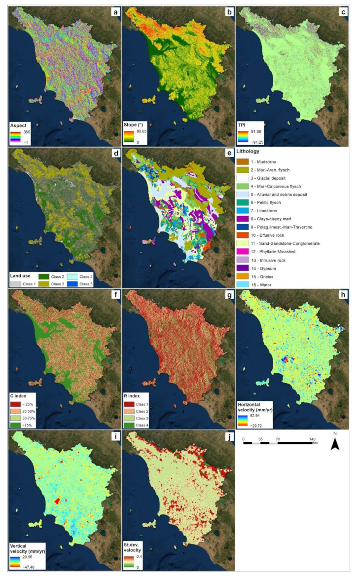
2.2.2. Predisposing Factors (PF)

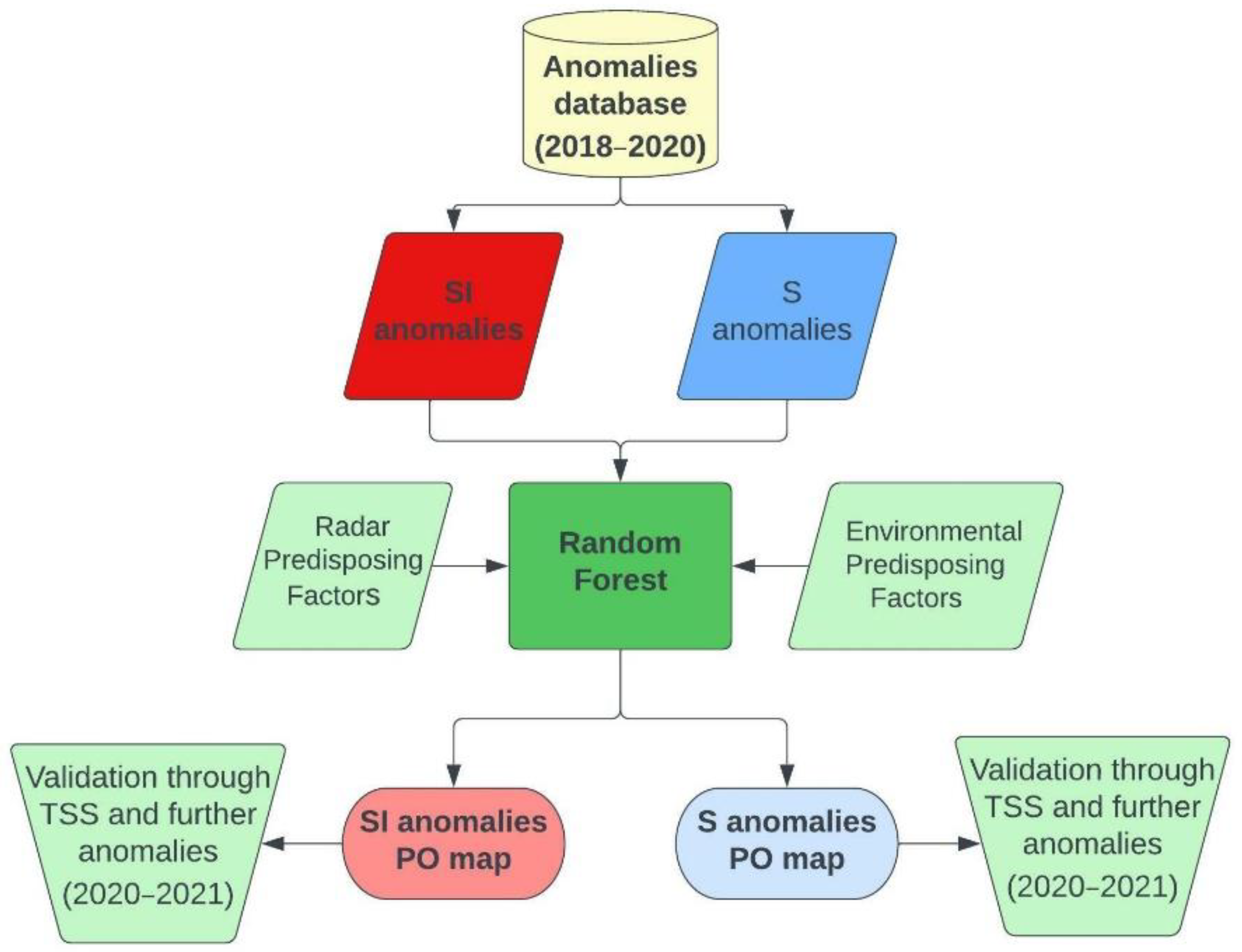
According to the morphological setting of the Tuscan territory and the main characteristic of the SAR system used to monitor the deformational scenario, ten PFs have been selected; five related to the first category and five to the second one. Namely, they are: Slope Aspect, Slope gradient, Topographic Position Index, Land Use and Lithology for the first class; and C-index, R-Index, Horizontal EW Velocity of displacement, Vertical velocity of displacement and Standard Deviation of the velocity of displacement for the second class (Figure 5).

The slope aspect (Figure 5a) is defined as the orientation of the Earth’s surface with respect to the sun. It is measured clockwise in degrees from 0 to 360, where 0 is north-facing, 90 is east-facing, 180 is south-facing, and 270 is west-facing. Flat areas have a value of −1. The slope aspect can play an important role in many factors controlling slope stability. Here, the slope aspect is also used to discriminate between flat and hilly areas, differentiating between subsidence and slope deformations.

The slope angle expresses the degree of incline of the topographic surface and may be one of the most significant factors for slope instabilities (Figure 5b).

The Topographic Position Index (TPI) is defined as the difference in elevation between a central pixel and the mean of its surrounding cells [58] (Figure 5c).

Land use–land cover corresponds to the ground surface cover (with natural or human-modified elements), which is connected with natural dynamics and human activities acting on the territory. The CORINE Land Cover (CLC) map of 2018 (the most updated available version) has been adopted for this work (Figure 5d). The third level products (the most detailed) have been used to be as precise as possible. To make the figure visible, the legend of Figure 5d is referred to in the first level. Class 1 indicates the artificial surfaces, class 2 the agricultural areas, class 3 the forest and semi-natural area, while classes 4 and 5 indicate the wetlands and the water bodies, respectively.

The lithological map has been taken from the regional cartographic service, available on the webGIS of the Tuscany region (Figure 5e).

The C-Index (Figure 5f), defined also as a visibility map [59], is a parameter expressing the percentage of the detectable movement by the SAR spaceborne systems. It can be calculated by applying the following formula [60], based on the geometric features of the slopes and the satellites (Equation (1)):

$$C = \left[N \times \cos S \times \sin \left(A - \pi /2\right)\right] + \left[\left(E \times (-1 \times \cos S \times \cos A - \pi /2)\right)+\left[H \times \cos S\right]\right]$$

(1)

where S is the slope angle while A is the slope aspect, and N, E and H are the LOS (Line Of Sight) directional cosines and can be calculated using the incidence angle and the LOS azimuth through the following formulas (Equation (2)):

$$\begin{gathered} E = \cos (\pi /2 - \theta )\times \cos (3\pi /2 - \alpha ) \\ N = \cos \left(\pi /2 - \theta \right) \times \cos (\pi - \alpha ) \\ H = \cos \theta \end{gathered}$$

(2)

where θ is the incidence angle and α is the satellite ground track angle. The four classes, as shown in Figure 5f, express the percentage of visibility (Class 1, with C values below 25%; Class 2, C values between 25 and 50%; Class 3 with C values between 50 and 75% and finally Class 4 with values > 75%).

The R-Index (Figure 5g) provides an estimation of the radar visibility of an area, by taking into account the radar geometry, the slope angle and slope orientation [61,62]. It is calculated as the ratio between the slant range and the ground range, starting from the geometry of the sensor and the geometry of the surface under analysis. The following equation (Equation (3)) defines the R-Index:

$$\mathrm{R} = -\sin \left(\arctan \left(\tan S \times \sin A\right) - \theta \right)$$

(3)

where S is the slope angle, A is the aspect and θ is the incident angle of the LOS. Class 1 of the R-index expresses those areas affected by a very low visibility, with distortion effects such as layover, foreshortening and shadow. Class 2 indicates R-Index < 30%, with a low amount of PSs (due to topographic effects); Class 3 and Class 4 are related to values of the R-Index between 30–50%, and over 50% (average and high amount of PSs), respectively.

The horizontal component (Figure 5h), along the EW direction, of the velocity of displacement (V_h) can be obtained through the combination of ascending and descending data, through the following equation (Equation (4)):

$$V_h = \frac{V_{asc}\cos {\theta }_{desc} - V_{desc}\cos {\theta }_{asc}}{\sin {\theta }_{asc} \cos {\theta }_{desc} - \sin {\theta }_{desc}\cos {\theta }_{asc}}$$

(4)

Furthermore, the vertical component (Figure 5i) can be obtained by combining the ascending and descending velocities of displacement, through the following equation (Equation (5)):

$$V_v = \frac{V_{asc}\sin {\theta }_{desc} - V_{desc}\sin {\theta }_{asc}}{\cos {\theta }_{asc}\sin {\theta }_{desc} - \cos {\theta }_{desc}\sin {\theta }_{asc}}$$

(5)

where V_asc, V_desc is the velocity from the ascending and descending geometries. V_v, V_h are the vertical and east–west values, θ_asc, θ_desc are the incidence angles for the ascending and descending orbits.

The standard deviation of the LOS velocity expresses the dispersion of the velocity from the mean value of the whole dataset (Figure 5j).

All the above-mentioned maps were rasterized with a 50 m cell size, which can be considered a good and balanced cell size for regional-scale studies and has already been adopted in the Tuscany region for landslide susceptibility [32].

2.3. Random Forest

RF is a nonparametric multivariate technique based on an ML algorithm [44]. It is a powerful method implemented in various scientific segments, such as economics, medicine, psychology, and in recent years has also been utilized in environmental modeling, for instance in the modeling of species distribution [63], and landslide susceptibility modeling [32,64]. The algorithm is based on the concepts of bootstrap aggregation (bagging) and classification or regression trees. Bootstrap aggregation takes uniform samples from an original dataset of predictors to create a subset of data that is allowed to have duplicated samples. From each sample, a tree is generated, thus splitting the data into subsets. However, in the RF algorithm, only a certain number of randomly selected points in the set are used to be split into subsets. In this way, the RF technique takes several bagged subsets from an original dataset and creates a certain amount of trees that are grown by randomly sampling points at each node. Once all the trees are grown, and a new value needs to be predicted, the values calculated by all the regression trees are averaged, assembling the final result. Indeed, each tree is developed to minimize classification errors, however the random selection influences the results, thus making a single-tree classification very unstable. For this reason, the RF-type methods make use of an ensemble of trees (the so-called “forest”), thereby ensuring model stability [32]. RF is an established and widely used technique in landslide studies as it outperforms traditional statistical methods, and it can be as effective as other ML methods [65,66,67]. Moreover, the RF technique is acknowledged for several advantages such as the joint use of categorical and numerical variables, the unnecessity of assumptions on the statistical distribution of the data and the capability of providing the statistical weight of each variable implemented. In this work, the RF algorithm implemented on the SDM (Spatial Distribution Modeling) package [68] on the R platform was adopted.

2.4. Modeling Validation

In order to validate the RF final products, the predictive accuracy of the model was assessed numerically by using the TSS (True Skill Statistic); TSS is a test that takes into account errors of omission and commission and ranges from −1 to +1, where the latter indicates a perfect performance [69]. The TSS method combines sensitivity and specificity so that both omission and commission errors are accounted for. This statistic compares the number of correct forecasts, minus those attributable to random guessing, to that of a hypothetical set of perfect forecasts [58]. For a 2 × 2 confusion matrix, TSS is defined as (Equation (6)):

$$\mathrm{TSS} = \frac{ad - bc}{\left(a + c\right)\left(b + d\right)} = \mathrm{Sensitivity} + \mathrm{Specificity} - 1$$

(6)

It can also be seen that TSS is not affected by the size of the validation set, and that two methods of equal performance have equal TSS scores. A further validation of the final modeled maps was performed by using a subset of the anomalies collected after 2020 (as described in Section 2.1). In this case, the anomalies were used and compared with the PO classes as determined by the RF model (see Section 3.4 for further information).

3. Results

RF modeling has been implemented in four different runs, by using the four datasets of anomalies, ascending and descending SI anomalies and ascending and descending S anomalies, while other anomalies are used as absence data. For the generation of the model, 10 environmental variables were adopted as PFs, as mentioned in Section 2.2. In addition, an eleventh parameter defined through the generation of random values all over the Tuscan territory, was created as a benchmark control variable to assess the significance of each PF. If the statistical weight of the random variable is higher than any other PF, the latter is discarded. In no cases, among the different runs, was the random map importance higher than the other PFs employed, thus confirming the whole selection. True Skill Statistic (TSS) has been considered to measure the accuracy of the RF model showing a good performance; in particular, an average value of 0.9 for landslides and 0.96 for subsidence has been obtained combining the results of the values of the ascending and descending orbits.

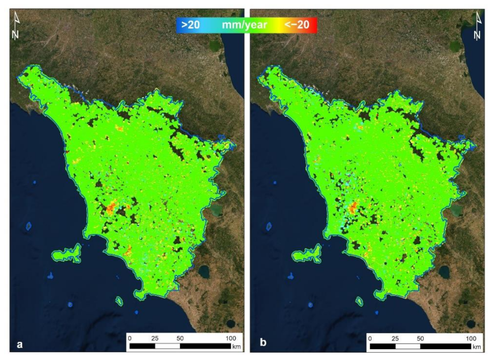
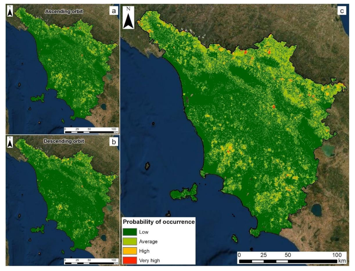
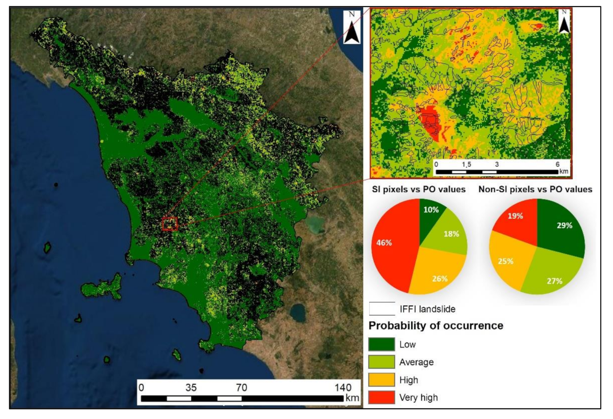
3.1. Slope Instability Anomalies Probability of Occurrence Map

As previously mentioned, two different SI anomalies Probability of Occurrence maps were generated, one using ascending anomalies and one for the descending, combined with the environmental and radar PFs. Both maps have values of PO between zero and one (Figure 6a,b), as computed by the Random Forest algorithm. These values have been divided into four classes: low probability (between 0 and 0.25); average (>0.25 and <0.5); high (>0.5 and <0.75); and very high (>0.75) for better visualization purposes and to compare with the control anomalies subset. The highest values of probability of occurrence of SI anomalies can be found over the main reliefs of the Apennine sector (especially over the Firenze and Pistoia side, with some spots over the Arezzo side), the Siena hilly area and the Mt. Amiata (Grosseto province) slopes. Especially in the descending map, some areas with higher values of probability can be found over the Apuan Alps (Massa–Carrara province). The RF algorithm is also capable of providing an assessment of the statistical weight of each PF within the model (

Table 2. Statistical weight of the predisposing factors.

Predisposing Factors	SI anomalies		S anomalies
	Ascending	Descending	Ascending	Descending
Aspect	1.95	2.78	0.84	0.51
C index	7.22	2.75	2.56	1.52
Lithology	7.25	15.88	1.90	3.74
Horizontal velocity	8.77	23.43	3.95	0.90
Land use	3.91	5.62	1.90	3.74
R index	1.53	1.91	0.84	0.42
Slope	14.12	9.04	12.65	11.83
St.dev. velocity	8.70	3.72	1.49	1.22
TPI	2.22	2.19	0.83	0.48
Vertical velocity	5.68	6.50	26.96	40.19

). As regards the ascending dataset map, the “heaviest” parameters are the slope gradient, followed by the horizontal velocity and the standard deviation of the velocity, while the R-Index, Slope Aspect and TPI show the lowest value. In the descending map, the horizontal velocity, lithology and slope gradient show the highest weight, and conversely, the R-Index, TPI and C-index show the lowest. A final SI anomalies probability of occurrence map has been produced by combining the ascending- and descending-related maps (Figure 6c). For the combination, the highest value of each cell has been taken and reported in the new map, so as to be more conservative and cautious. The spatial pattern of the different values of PO is extremely similar to that reported for the “single” maps.

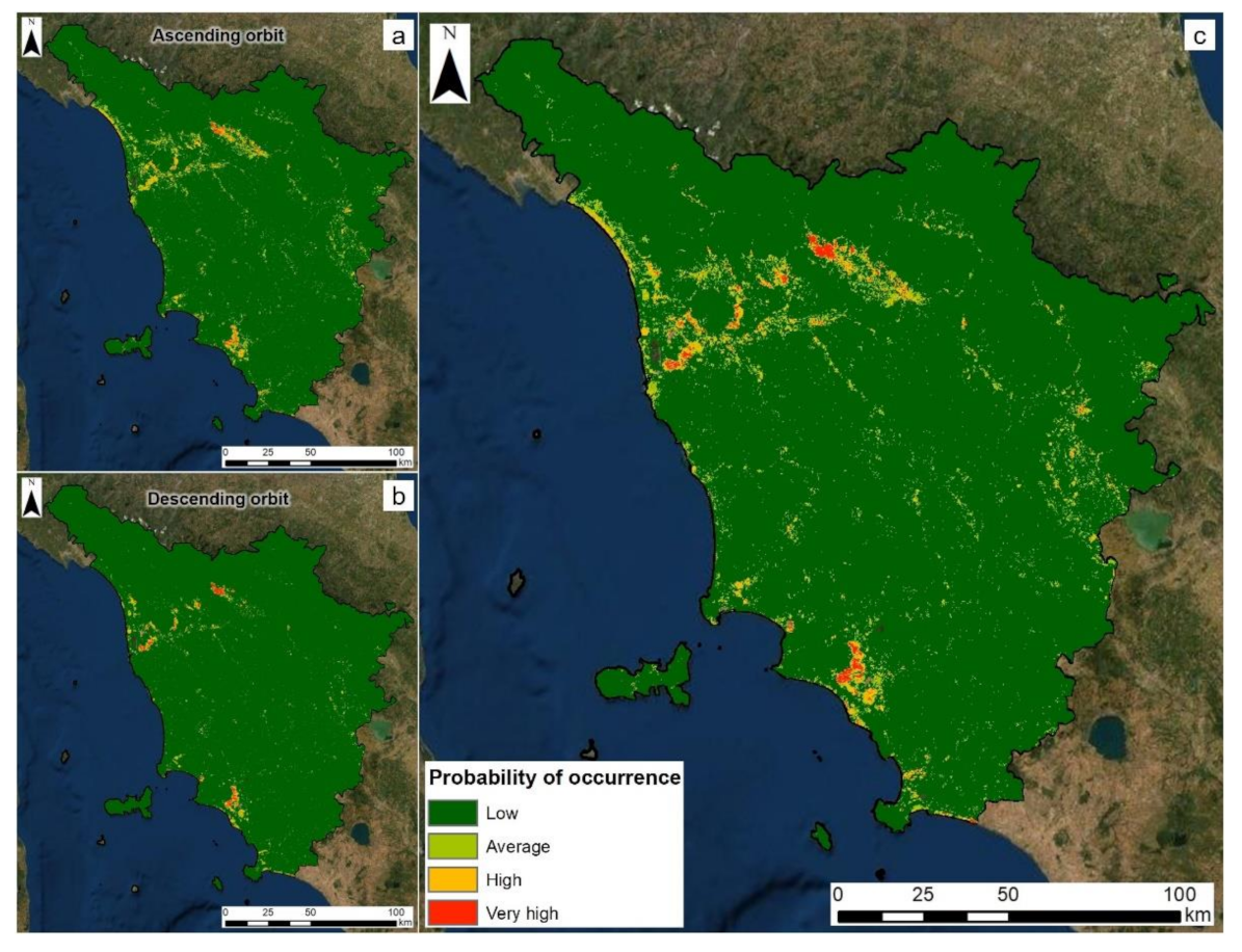
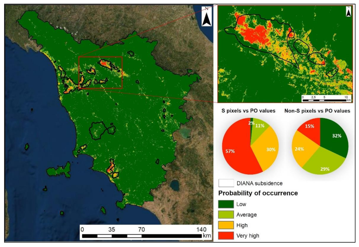
3.2. Subsidence Anomalies Probability of Occurrence Map

For the subsidence anomalies, PO two maps were redacted as well, according to the ascending and descending anomalies and radar-based PFs (Figure 7a,b). Furthermore, in this case, values range between zero and one and have been subdivided into four classes. The distribution of the different values of PO is more or less similar between the ascending and the descending map, as expected for subsidence phenomena, with extensive higher values over the main plains, in particular over the Firenze–Prato–Pistoia plain and the Pisa-Livorno and Grosseto coastal sectors. As for the parameter weight (Table 2), as assessed by the RF model, in the ascending map the role of Vertical Velocity, Land Cover and slope gradient is higher than the rest of the PFs, while the R-Index and aspect do not show any relative importance; in the descending map, the main role is given by the vertical velocity, followed by the slope and land cover, while no significance is given by the R-Index and TPI. The two-orbit maps were combined to get a final map, which has the same spatial class distribution pattern (Figure 7c).

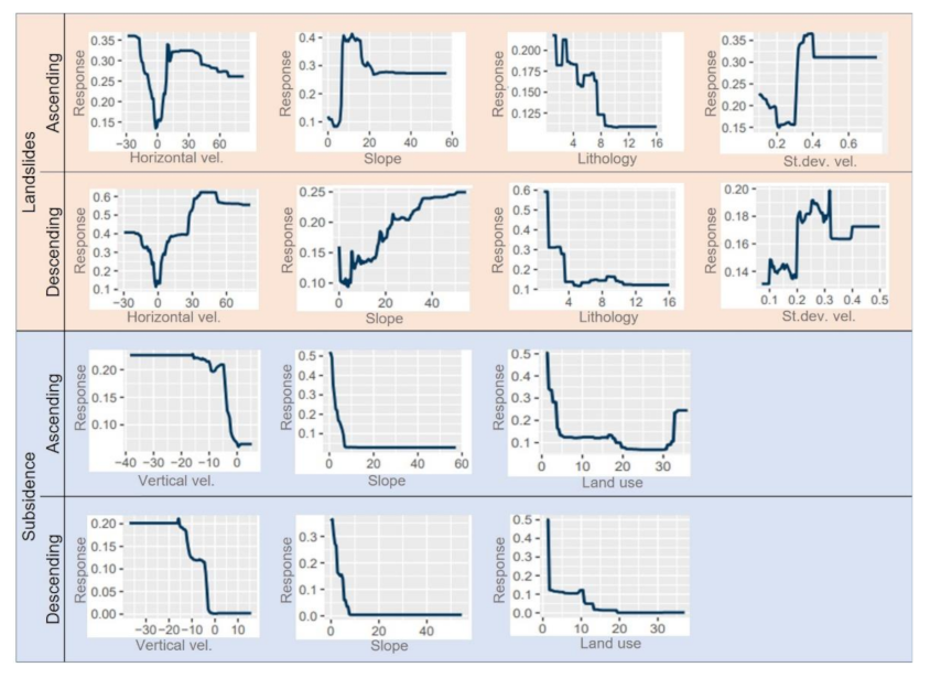
3.3. Response Curves

One of the abilities of the RF application is to represent the response curves of each model. A response curve is used to quantify the behavior of variables and to recognize the relationships between each conditioning factor and the modeling [70]. In the case of the SI probability of occurrence map, the response curves of the most valuable PFs, i.e., horizontal velocity, slope gradient, lithology and velocity standard deviation, show a higher response of some values with respect to others (Figure 8). For instance, in the descending map, the horizontal velocities with a higher response are those > +30 mm/year, while in the ascending map a higher response is given by the velocities < −25 mm/year. The slope gradient response curves show higher values between 10 and 20° in the case of the ascending map, while higher than 30° for the descending one. Instead, the standard deviation of the ascending map has a peak with the value of 0.4; the lithologies with a higher response in the descending PO map are the mudstone and marly arenaceous flysch formations. For the subsidence PO map, the main role, as evidenced in Section 3.2, is provided by three PFs, the vertical velocity, the slope gradient and the land cover. The response curves of these three parameters are very similar between the ascending and the descending map (Figure 8): the vertical velocity curve shows a higher response with values < −10 mm/year, as well as generally low slope values (below 5°) that give a better response. Finally, the classes of land cover showing a high response are those related to the artificial surfaces (class 1 of the Corine Land Cover classification) in both maps.

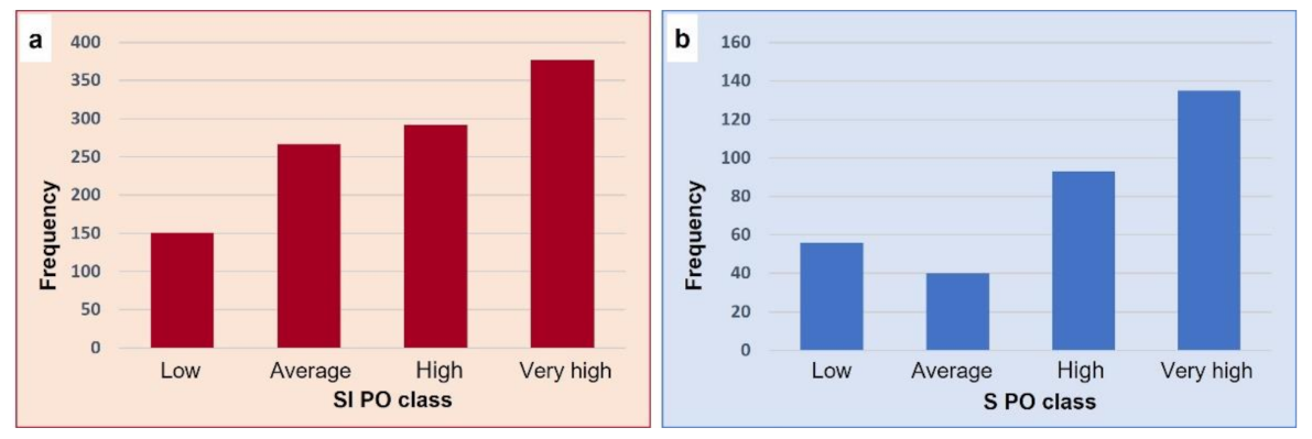
3.4. Cross-Validation of PO Maps

As described in Section 2.2.1, 1087 SI anomalies collected between January 2020 and April 2021 have been used to validate the final PO maps (Figure 9). An increasing trend can be observed in the numerical distribution. The highest frequency is seen in the very high PO class (377 out of 1087), followed by high PO, with 27% (292), average PO, with about 25% (267) and, lastly, low PO with 14% (151). On the other hand, 327 S anomalies between May 2020 and April 2021 were used to validate the merged final maps. In detail, 138 anomalies fall within the very high PO class, representing about 42% of the total, 93 in the class high PO (28%), while the average and low PO classes count 40 and 56 anomalies, respectively (12 and 17% of the total).

To evaluate the spatial distribution of the various PO classes, a cross-comparison with official landslide and subsidence inventories was performed. Indeed, IFFI landslide (Inventario dei Fenomeni Franosi in Italia, Landslide Inventory in Italy) [71,72] and DIANA subsidence (Dati Interferometrici per l’ANalisi Ambientale—Interferometric data for environmental analysis [54,73]) inventories were intersected with the pixels of the SI and S PO maps, respectively. In the first case (SI anomalies PO map), the number of pixels within and outside the inventoried landslide was evaluated, analyzing the number of cells for each class of PO (Figure 10). The total number of PO pixels within landslide polygons is 982,906, of which 12,413 (1.26% of the total number) have a value of PO between 0.75–1 (very high), 47,801 are high (4.86%), 440,518 in the average class (44.82%) and 482,174 (49.06%) in the low class. The same analysis was performed on the non-landslide cells, and a very low percentage of cells falls within the higher PO classes (0.24% and 2.15% for classes very high and high, respectively), while much higher concentrations can be found over the lower classes (30.47 and 67.13% for class average and low, respectively). The number of cells for each PO class was also analyzed according to the total number of cells for the whole Tuscany territory (i.e., dividing the number of pixels with a certain PO class within the landslide and the total number of pixels with a certain PO value). Such analysis has revealed that, in the case of the SI PO cells overlapped on landslide polygons, the higher “influence” is related to the very high class (46.24% of the total), thus these values decrease proportionally with the class values. Conversely, the cells over the non-landslide areas show a balance among the different classes of probability of occurrence, with a percentage lower than 30% in all four classes (19 and 25% over the very high and high classes).

The same analysis was performed on the S PO cells over the subsidence areas as defined by the DIANA inventory (Figure 11). As regards the pixels over the subsidence areas, the highest percentage is given by the PO low class (55.66%) and the lowest by PO very high class (10.61%), however, normalizing this value with the total number of cells in Tuscany, the trend becomes the opposite, with the highest weight given by very high class (57.36%) and the lowest by the low class (1.57%). A similar trend can be observed in the overlap between S PO pixels and non-subsiding areas: analyzing the concentration of pixels in non-subsiding areas, 95% fall within the lowest class (values of PO between 0–0.25), however, normalizing the number of these pixels with the total number of pixels, the percentages are balanced between the different classes of PO. A summary of the comparison between PO cells and landslide and subsidence inventories is reported in

Table 3. Summary of the results of the comparison between PO cell values and landslide and subsidence inventories.

	SI PO Class
	Low Probability (0–25%)	Average Probability (25–50%)	High Probability (50–75%)	Very High Probability (75–100%)
Landslide inventory	9.77%	18.16%	25.83%	46.24%
No Landslide inventory	28.99%	26.79%	24.78%	19.43%
	S PO Class
	Low Probability (0–25%)	Average Probability (25–50%)	High Probability (50–75%)	Very High Probability (75–100%)
Subsidence inventory	1.57%	10.56%	30.51%	57.36%
No Subsidence inventory	31.99%	29.31%	23.36%	15.35%

.

4. Discussion

The joint use of advanced Earth Observation products, fostered by the launch of groundbreaking spaceborne missions such as the Sentinel-1, and Machine Learning algorithms, is gaining much more consideration in studies dealing with the analysis of geohazards. The use of remote sensing SAR data, in particular of continuous information such as in the case of the Tuscany region, is a valid support for the constant and up-to-date near-real-time monitoring of wide areas. On the other hand, the implementation of statistical-probabilistic methodologies, such as Random Forest, is a considerable development for the preparation of highly accurate provisional models. In recent years, the combination of these two techniques has provided significant results for landslide susceptibility mapping, as represented by the works of [41], which used the SBAS data to refine a susceptibility model of landslides along the Karakorum highway (Chinese Himalaya), or Ilia, et al. [74,75], which investigated the relationship between land subsidence and the spatiotemporal pattern of groundwater in western Thessaly (Greece).

In this work, RF and InSAR data have been jointly used for the assessment of the probability of occurrence of anomalies of movement, i.e., acceleration of deceleration of displacement as detected by SAR satellites. Since the launch of the continuous monitoring system in October 2016, based on the exclusive use of Sentinel-1 data for the whole territory of Tuscany, more than 50,000 anomalies were collected and interpreted. In Confuorto, et al. [28], an analysis was conducted on the distribution of one year (July 2019–July 2020) of anomalies in three Italian regions (including Tuscany) where the operational service was active. The results showed a substantial connection between the spatial disposition of the anomalies and the physiographic, environmental, and geological settings of each region. Following these outcomes, the objective of this work has been to set up a methodology, which allows us to identify the main factors and the main processes that lead to the changes in the displacement trend and to estimate the occurrence probability of anomalies of movement, and thus, identify the most prone areas.

The RF model was selected for this aim since it is capable of producing good predictions, handling large datasets efficiently and with a high level of accuracy, as testified by the different validation approaches tested in this work. Indeed, TSS test values showed a good performance of the RF model (TSS = 0.9 for landslides and TSS = 0.96 for subsidence); additionally, the anomalies collected in a second phase (between May 2020 and April 2021 for S and between January 2020 and April 2021 for SI) were used to validate the PO models. The cross-validation revealed that generally about 70% of these anomalies fall within the higher classes of PO, thus demonstrating the good predictive performance of the maps and that the anomalies are very often recurrent and persistent in space and over time.

Another key aspect of RF is the capability of estimating the variable importance, providing valuable insights that help us to interpret the models. In this work, classical environmental and geomorphological features, the expression of the territory under analysis, were coupled with radar features, typical of the SAR data from which the anomalies were generated. These parameters can be considered a synthesis of the main aspects leading to the anomaly’s generation, the latter being dependent on either the territory physiography, or geology and land use, as well as the radar visibility and characteristics. In the case of SI anomalies, the most significant factors are the slope gradient, which is undoubtedly a diffuse conditioning element for landsliding, and the horizontal projection of the LOS velocity, confirming that the major component of the movement is along the horizontal axis (even if with SAR, only the E-W component can be obtained). The lithology also assumes a certain role, thus confirming the geological control over the landslide displacements and their acceleration, as well as the standard deviation of the velocity, which implies that the higher this value is, the more likely it is that an abrupt acceleration can be connected with a sudden reactivation of a mass movement along a hillslope or mountainside. With regard to the S anomalies PO map, three factors are the most important: the vertical velocity, the slope gradient, and the land use. In both cases (ascending and descending map), the first is the factor with the highest weight, which is used by the RF algorithm to identify subsidence phenomena as they are essentially a vertical displacement. The significance of the slope gradient is given by the flat morphology (thus very low values of slope), where generally subsidence occurs. Finally, the land use assumes a notable function, since most of the anomalies are verified in an urban setting, where most of the accelerations have a seasonal character and are mostly due to overexploitation of underground resources (such as in the cases of Montemurlo, Prato province, as highlighted by Del Soldato, et al. [27]) or where the building load induces severe settlements (e.g., in Pisa, [76], or on the freight terminal of Guasticce, Livorno province [77]).

The role of each PF and the value of each variable can also be estimated through the response curves, as seen in Section 3.3. Their implementation provides a valuable support for the understanding of the model and of the variables. In the SI PO map, the response curves of the most significant PF, highlight that SI anomalies generally occur in areas with high horizontal velocities of displacement (higher than 20 mm/year), and with a variable slope gradient (between 10 and 30°); as regards the lithology, the mudstone and the flysch formations give a higher response, since landslides occur very often in Tuscany and are more sensitive to acceleration in such terrains, as in the case of Carpineta (Pistoia province, Raspini, et al. [77]) and as observed by Rosi, et al. [53] across the entire Tuscan regional territory. For the S PO map, the response curves highlighted that generally the vertical velocity values should not be necessarily very high, and furthermore, S anomalies are likely to occur over flat areas (as testified by the higher response of very low slope gradient values). As previously mentioned, as concerns the land use, generally SI anomalies are more likely to occur over urban areas, as is evident from the response curve of the CLC map.

Finally, the comparison of the anomalies PO map values with the existing landslide and subsidence inventories demonstrated that SI anomalies may not necessarily only occur in already inventoried landslides, but they may also be generated in unknown slopes (almost 45% of the non-landslide pixels have high and very high PO values).The S anomalies show a great percentage of the pixel within subsidence inventoried areas having high and very high PO values (about 90%), while a minor percentage of non-subsidence pixels (about 38%) are found. This result is also significant, considering that the subsidence inventory is dated back to 2013, and thus has not been updated. This confirms that accelerations due to SI may take place in many slope sectors and that inventories should be updated frequently, while subsidence accelerations very often occur in well-known areas, and they are induced by seasonal fluctuations or by settlements due to the urban sprawl.

5. Conclusions

The availability of an unprecedented amount of spaceborne information, as represented by the Sentinel-1 imagery, is a turning point for the monitoring of geohazards, and along with a reduced revisit time of up to six days, made possible the beginning of operational continuous monitoring services based exclusively on SAR (Synthetic Aperture Radar) data. Tuscany is at the forefront in this sense as it was the first region to rely on this kind of service, which is based on the identification of the so-called anomalies of movement, i.e., measurement points, derived from MTInSAR (Multi Temporal Interferometry SAR) techniques, by means of a changing deformation trend through a data-mining algorithm. In this work, the probability of occurrence of landslide- and subsidence-related anomalies was assessed through the adoption of Machine Learning Random Forest algorithms. Two maps were generated, one estimating the probability of occurrence for Tuscany to have Slope Instability (SI) anomalies, and one Subsidence (S) anomalies. A total of ten environmental factors were selected and included in the modeling; five connected to the radar data and five to the morphology and geology of the study area. The final maps were validated through the overlap with further and subsequent anomalies and compared with the landslide and subsidence inventories available. In the first case, more than 70% of the control anomalies fall within the higher classes of probability of occurrence, both for SI and for S. As for the second case, the comparison of SI probability of occurrence values with inventoried landslide showed that anomalies can be generated even in non-inventoried areas (as testified by almost 45% of the non-landslide pixels having high and very high probability of occurrence values); in the case of S anomalies, a minor percentage of non-subsidence pixels (about 38%) were found, showing that most of the accelerations were within well-known subsiding areas. The adoption of a ML method also enabled us to comprehend the main driving forces that lead to the changes in the deformation trends, highlighting the major role of predisposing factors such as the slope gradient, the horizontal or vertical projection of the velocity of displacement, the land cover and the lithology. Further improvements can be made regarding the choice of the parameters to consider, whose selection could be extended to other environmental factors, as well as the replication of the analysis, even with other ML methods, over other Italian regions. The adoption of a map for assessing the probability of occurrence of MTInSAR anomalies may represent a step forward for the understanding of deformational phenomena and may serve as an enhanced geohazard prevention measurement, to be periodically updated and refined in order to have the most precise as possible knowledge of the territory.

References

1. Franceschini, R.; Rosi, A.; Catani, F.; Casagli, N. Exploring a landslide inventory created by automated web data mining: The case of Italy. Landslides 2022, 19, 1–13. [Google Scholar] [CrossRef]
2. Lanari, R.; Bonano, M.; Casu, F.; Luca, C.D.; Manunta, M.; Manzo, M.; Onorato, G.; Zinno, I. Automatic generation of sentinel-1 continental scale DInSAR deformation time series through an extended P-SBAS processing pipeline in a cloud computing environment. Remote Sens. 2020, 12, 2961. [Google Scholar] [CrossRef]
3. Crosetto, M.; Solari, L.; Mróz, M.; Balasis-Levinsen, J.; Casagli, N.; Frei, M.; Oyen, A.; Moldestad, D.A.; Bateson, L.; Guerrieri, L. The evolution of wide-area dinsar: From regional and national services to the European ground motion service. Remote Sens. 2020, 12, 2043. [Google Scholar] [CrossRef]
4. Costantini, M.; Ferretti, A.; Minati, F.; Falco, S.; Trillo, F.; Colombo, D.; Novali, F.; Malvarosa, F.; Mammone, C.; Vecchioli, F. Analysis of surface deformations over the whole Italian territory by interferometric processing of ERS, Envisat and COSMO-SkyMed radar data. Remote Sens. Environ. 2017, 202, 250–275. [Google Scholar] [CrossRef]
5. Di Martire, D.; Paci, M.; Confuorto, P.; Costabile, S.; Guastaferro, F.; Verta, A.; Calcaterra, D. A nation-wide system for landslide mapping and risk management in Italy: The second Not-ordinary Plan of Environmental Remote Sensing. Int. J. Appl. Earth Obs. Geoinf. 2017, 63, 143–157. [Google Scholar] [CrossRef]
6. Novellino, A.; Cigna, F.; Brahmi, M.; Sowter, A.; Bateson, L.; Marsh, S. Assessing the Feasibility of a National InSAR Ground Deformation Map of Great Britain with Sentinel-1. Geosciences 2017, 7, 19. [Google Scholar] [CrossRef] [Green Version]
7. Kalia, A.; Frei, M.; Lege, T. A Copernicus downstream-service for the nationwide monitoring of surface displacements in Germany. Remote Sens. Environ. 2017, 202, 234–249. [Google Scholar] [CrossRef]
8. Zhang, Y.; Meng, X.; Jordan, C.; Novellino, A.; Dijkstra, T.; Chen, G. Investigating slow-moving landslides in the Zhouqu region of China using InSAR time series. Landslides 2018, 15, 1–17. [Google Scholar] [CrossRef]
9. Montalti, R.; Solari, L.; Bianchini, S.; Del Soldato, M.; Raspini, F.; Casagli, N. A Sentinel-1-based clustering analysis for geo-hazards mitigation at regional scale: A case study in Central Italy. Geomat. Nat. Hazards Risk 2019, 10, 2257–2275. [Google Scholar] [CrossRef] [Green Version]
10. Bekaert, D.P.S.; Handwerger, A.L.; Agram, P.; Kirschbaum, D.B. InSAR-based detection method for mapping and monitoring slow-moving landslides in remote regions with steep and mountainous terrain: An application to Nepal. Remote Sens. Environ. 2020, 249, 111983. [Google Scholar] [CrossRef]
11. Liu, L.M.; Yu, J.; Chen, B.B.; Wang, Y.B. Urban subsidence monitoring by SBAS-InSAR technique with multi-platform SAR images: A case study of Beijing Plain, China. Eur. J. Remote Sens. 2020, 53, 141–153. [Google Scholar] [CrossRef] [Green Version]
12. Meng, Q.; Confuorto, P.; Peng, Y.; Raspini, F.; Bianchini, S.; Han, S.; Liu, H.; Casagli, N. Regional recognition and classification of active loess landslides using two-dimensional deformation derived from Sentinel-1 interferometric radar data. Remote Sens. 2020, 12, 1541. [Google Scholar] [CrossRef]
13. Crippa, C.; Valbuzzi, E.; Frattini, P.; Crosta, G.B.; Spreafico, M.C.; Agliardi, F. Semi-automated regional classification of the style of activity of slow rock-slope deformations using PS InSAR and SqueeSAR velocity data. Landslides 2021, 18, 2445–2463. [Google Scholar] [CrossRef]
14. Bozzano, F.; Mazzanti, P.; Perissin, D.; Rocca, A.; De Pari, P.; Discenza, M.E. Basin Scale Assessment of Landslides Geomorphological Setting by Advanced InSAR Analysis. Remote Sens. 2017, 9, 267. [Google Scholar] [CrossRef] [Green Version]
15. Confuorto, P.; Di Martire, D.; Centolanza, G.; Iglesias, R.; Mallorqui, J.J.; Novellino, A.; Plank, S.; Ramondini, M.; Thuro, K.; Calcaterra, D. Post-failure evolution analysis of a rainfall-triggered landslide by multi-temporal interferometry SAR approaches integrated with geotechnical analysis. Remote Sens. Environ. 2017, 188, 51–72. [Google Scholar] [CrossRef]
16. Dong, J.; Liao, M.; Xu, Q.; Zhang, L.; Tang, M.; Gong, J. Detection and displacement characterization of landslides using multi-temporal satellite SAR interferometry: A case study of Danba County in the Dadu River Basin. Eng. Geol. 2018, 240, 95–109. [Google Scholar] [CrossRef]
17. Ezquerro, P.; Del Soldato, M.; Solari, L.; Tomás, R.; Raspini, F.; Ceccatelli, M.; Fernández-Merodo, J.A.; Casagli, N.; Herrera, G. Vulnerability assessment of buildings due to land subsidence using InSAR data in the ancient historical city of Pistoia (Italy). Sensors 2020, 20, 2749. [Google Scholar] [CrossRef]
18. Tzouvaras, M.; Danezis, C.; Hadjimitsis, D.G. Differential SAR Interferometry Using Sentinel-1 Imagery-Limitations in Monitoring Fast Moving Landslides: The Case Study of Cyprus. Geosciences 2020, 10, 236. [Google Scholar] [CrossRef]
19. Tomás, R.; Romero, R.; Mulas, J.; Marturià, J.J.; Mallorquí, J.J.; Lopez-Sanchez, J.M.; Herrera, G.; Gutiérrez, F.; González, P.J.; Fernández, J. Radar interferometry techniques for the study of ground subsidence phenomena: A review of practical issues through cases in Spain. Environ. Earth Sci. 2014, 71, 163–181. [Google Scholar] [CrossRef] [Green Version]
20. Dong, S.C.; Samsonov, S.; Yin, H.W.; Ye, S.J.; Cao, Y.R. Time-series analysis of subsidence associated with rapid urbanization in Shanghai, China measured with SBAS InSAR method. Environmental Earth Sciences 2014, 72, 677–691. [Google Scholar] [CrossRef]
21. Dong, J.; Zhang, L.; Tang, M.; Liao, M.; Xu, Q.; Gong, J.; Ao, M. Mapping landslide surface displacements with time series SAR interferometry by combining persistent and distributed scatterers: A case study of Jiaju landslide in Danba, China. Remote Sens. Environ. 2018, 205, 180–198. [Google Scholar] [CrossRef]
22. Solari, L.; Del Soldato, M.; Raspini, F.; Barra, A.; Bianchini, S.; Confuorto, P.; Casagli, N.; Crosetto, M. Review of satellite interferometry for landslide detection in Italy. Remote Sens. 2020, 12, 1351. [Google Scholar] [CrossRef]
23. Wang, Y.; Liu, D.; Dong, J.; Zhang, L.; Guo, J.; Liao, M.; Gong, J. On the applicability of satellite SAR interferometry to landslide hazards detection in hilly areas: A case study of Shuicheng, Guizhou in Southwest China. Landslides 2021, 18, 2609–2619. [Google Scholar] [CrossRef]
24. Ferretti, A.; Fumagalli, A.; Novali, F.; Prati, C.; Rocca, F.; Rucci, A. A new algorithm for processing interferometric data-stacks: SqueeSAR. IEEE Trans. Geosci. Remote Sens. 2011, 49, 3460–3470. [Google Scholar] [CrossRef]
25. Casu, F.; Elefante, S.; Imperatore, P.; Zinno, I.; Manunta, M.; De Luca, C.; Lanari, R. SBAS-DInSAR parallel processing for deformation time-series computation. IEEE J. Sel. Top. Appl. Earth Obs. Remote Sens. 2014, 7, 3285–3296. [Google Scholar] [CrossRef]
26. Raspini, F.; Bianchini, S.; Ciampalini, A.; Del Soldato, M.; Solari, L.; Novali, F.; Del Conte, S.; Rucci, A.; Ferretti, A.; Casagli, N. Continuous, semi-automatic monitoring of ground deformation using Sentinel-1 satellites. Sci. Rep. 2018, 8, 1–11. [Google Scholar] [CrossRef] [Green Version]
27. Del Soldato, M.; Solari, L.; Raspini, F.; Bianchini, S.; Ciampalini, A.; Montalti, R.; Ferretti, A.; Pellegrineschi, V.; Casagli, N. Monitoring ground instabilities using SAR satellite data: A practical approach. ISPRS Int. J. Geo-Inf. 2019, 8, 307. [Google Scholar] [CrossRef] [Green Version]
28. Confuorto, P.; Del Soldato, M.; Solari, L.; Festa, D.; Bianchini, S.; Raspini, F.; Casagli, N. Sentinel-1-based monitoring services at regional scale in Italy: State of the art and main findings. Int. J. Appl. Earth Obs. Geoinf. 2021, 102, 102448. [Google Scholar] [CrossRef]
29. Zhao, G.; Pang, B.; Xu, Z.; Peng, D.; Xu, L. Assessment of urban flood susceptibility using semi-supervised machine learning model. Sci. Total. Environ. 2019, 659, 940–949. [Google Scholar] [CrossRef]
30. Youssef, A.M.; Pradhan, B.; Jebur, M.N.; El-Harbi, H.M. Landslide susceptibility mapping using ensemble bivariate and multivariate statistical models in Fayfa area, Saudi Arabia. Environ. Earth Sci. 2015, 73, 3745–3761. [Google Scholar] [CrossRef]
31. Merghadi, A.; Yunus, A.P.; Dou, J.; Whiteley, J.; ThaiPham, B.; Bui, D.T.; Avtar, R.; Abderrahmane, B.J.E.-S.R. Machine learning methods for landslide susceptibility studies: A comparative overview of algorithm performance. Earth-Sci. Rev. 2020, 207, 103225. [Google Scholar] [CrossRef]
32. Catani, F.; Lagomarsino, D.; Segoni, S.; Tofani, V. Landslide susceptibility estimation by random forests technique: Sensitivity and scaling issues. Nat. Hazards Earth Syst. Sci. 2013, 13, 2815–2831. [Google Scholar] [CrossRef] [Green Version]
33. Marjanović, M.; Kovačević, M.; Bajat, B.; Voženílek, V. Landslide susceptibility assessment using SVM machine learning algorithm. Eng. Geol. 2011, 123, 225–234. [Google Scholar] [CrossRef]
34. Ermini, L.; Catani, F.; Casagli, N. Artificial neural networks applied to landslide susceptibility assessment. Geomorphology 2005, 66, 327–343. [Google Scholar] [CrossRef]
35. Wang, Y.; Fang, Z.; Hong, H. Comparison of convolutional neural networks for landslide susceptibility mapping in Yanshan County, China. Sci. Total. Environ. 2019, 666, 975–993. [Google Scholar] [CrossRef]
36. Felicísimo, Á.M.; Cuartero, A.; Remondo, J.; Quirós, E. Mapping landslide susceptibility with logistic regression, multiple adaptive regression splines, classification and regression trees, and maximum entropy methods: A comparative study. Landslides 2013, 10, 175–189. [Google Scholar] [CrossRef]
37. Raso, E.; Di Martire, D.; Cevasco, A.; Calcaterra, D.; Scarpellini, P.; Firpo, M. Evaluation of prediction capability of the MaxEnt and Frequency Ratio methods for landslide susceptibility in the Vernazza catchment (Cinque Terre, Italy). In Applied Geology; Springer: Berlin/Heidelberg, Germany, 2020; pp. 299–316. [Google Scholar]
38. Bianchini, S.; Solari, L.; Del Soldato, M.; Raspini, F.; Montalti, R.; Ciampalini, A.; Casagli, N. Ground Subsidence Susceptibility (GSS) Mapping in Grosseto Plain (Tuscany, Italy) Based on Satellite InSAR Data Using Frequency Ratio and Fuzzy Logic. Remote Sens. 2019, 11, 2015. [Google Scholar] [CrossRef] [Green Version]
39. Hakim, W.L.; Achmad, A.R.; Lee, C.W. Land Subsidence Susceptibility Mapping in Jakarta Using Functional and Meta-Ensemble Machine Learning Algorithm Based on Time-Series InSAR Data. Remote Sens. 2020, 12, 3627. [Google Scholar] [CrossRef]
40. Mohammady, M.; Pourghasemi, H.R.; Amiri, M. Land subsidence susceptibility assessment using random forest machine learning algorithm. Environ. Earth Sci. 2019, 78, 1–12. [Google Scholar] [CrossRef]
41. Zhao, F.; Meng, X.; Zhang, Y.; Chen, G.; Su, X.; Yue, D. Landslide susceptibility mapping of karakorum highway combined with the application of SBAS-InSAR technology. Sensors 2019, 19, 2685. [Google Scholar] [CrossRef] [Green Version]
42. Ciampalini, A.; Raspini, F.; Lagomarsino, D.; Catani, F.; Casagli, N. Landslide susceptibility map refinement using PSInSAR data. Remote Sens. Environ. 2016, 184, 302–315. [Google Scholar] [CrossRef]
43. Novellino, A.; Cesarano, M.; Cappelletti, P.; Di Martire, D.; Di Napoli, M.; Ramondini, M.; Sowter, A.; Calcaterra, D. Slow-moving landslide risk assessment combining Machine Learning and InSAR techniques. Catena 2021, 203, 105317. [Google Scholar] [CrossRef]
44. Breiman, L. Random forests. Mach. Learn. 2001, 45, 5–32. [Google Scholar] [CrossRef] [Green Version]
45. Duro, D.C.; Franklin, S.E.; Dubé, M.G. A comparison of pixel-based and object-based image analysis with selected machine learning algorithms for the classification of agricultural landscapes using SPOT-5 HRG imagery. Remote Sens. Environ. 2012, 118, 259–272. [Google Scholar] [CrossRef]
46. De Oliveira, G.G.; Ruiz, L.F.C.; Guasselli, L.A.; Haetinger, C. Random forest and artificial neural networks in landslide susceptibility modeling: A case study of the Fão River Basin, Southern Brazil. Nat. Hazards 2019, 99, 1049–1073. [Google Scholar] [CrossRef]
47. Sun, D.; Xu, J.; Wen, H.; Wang, D. Assessment of landslide susceptibility mapping based on Bayesian hyperparameter optimization: A comparison between logistic regression and random forest. Eng. Geol. 2021, 281, 105972. [Google Scholar] [CrossRef]
48. Canavesi, V.; Segoni, S.; Rosi, A.; Ting, X.; Nery, T.; Catani, F.; Casagli, N. Different approaches to use morphometric attributes in landslide susceptibility mapping based on meso-scale spatial units: A case study in Rio de Janeiro (Brazil). Remote Sens. 2020, 12, 1826. [Google Scholar] [CrossRef]
49. Boccaletti, M.; Guazzone, G. Remnant arcs and marginal basins in the Cainozoic development of the Mediterranean. Nature 1974, 252, 18–21. [Google Scholar] [CrossRef]
50. Bortolotti, V. The Tuscany–Emilian Apennine; BEMA Editrice: Milano, Italy, 1992; Volume 4. [Google Scholar]
51. Vai, F.; Martini, I.P. Anatomy of an Orogen: The Apennines and Adjacent Mediterranean Basins; Springer: Berlin/Heidelberg, Germany, 2013. [Google Scholar]
52. Segoni, S.; Battistini, A.; Rossi, G.; Rosi, A.; Lagomarsino, D.; Catani, F.; Moretti, S.; Casagli, N. An operational landslide early warning system at regional scale based on space–time-variable rainfall thresholds. Nat. Hazards Earth Syst. Sci. 2015, 15, 853–861. [Google Scholar] [CrossRef] [Green Version]
53. Rosi, A.; Tofani, V.; Tanteri, L.; Tacconi Stefanelli, C.; Agostini, A.; Catani, F.; Casagli, N. The new landslide inventory of Tuscany (Italy) updated with PS-InSAR: Geomorphological features and landslide distribution. Landslides 2018, 15, 5–19. [Google Scholar] [CrossRef] [Green Version]
54. Rosi, A.; Tofani, V.; Agostini, A.; Tanteri, L.; Stefanelli, C.T.; Catani, F.; Casagli, N. Subsidence mapping at regional scale using persistent scatters interferometry (PSI): The case of Tuscany region (Italy). Int. J. Appl. Earth Obs. Geoinf. 2016, 52, 328–337. [Google Scholar] [CrossRef]
55. Solari, L.; Ciampalini, A.; Raspini, F.; Bianchini, S.; Zinno, I.; Bonano, M.; Manunta, M.; Moretti, S.; Casagli, N. Combined Use of C-and X-Band SAR Data for Subsidence Monitoring in an Urban Area. Geosciences 2017, 7, 21. [Google Scholar] [CrossRef] [Green Version]
56. Del Soldato, M.; Farolfi, G.; Rosi, A.; Raspini, F.; Casagli, N. Subsidence Evolution of the Firenze-Prato-Pistoia Plain (Central Italy) Combining PSI and GNSS Data. Remote Sens. 2018, 10, 1146. [Google Scholar] [CrossRef] [Green Version]
57. Ceccatelli, M.; Del Soldato, M.; Solari, L.; Fanti, R.; Mannori, G.; Castelli, F. Numerical modelling of land subsidence related to groundwater withdrawal in the Firenze-Prato-Pistoia basin (central Italy). Hydrogeol. J. 2021, 29, 629–649. [Google Scholar] [CrossRef]
58. Wilson, J.P.; Gallant, J.C. Digital terrain analysis. Terrain Anal. Princ. Appl. 2000, 6, 1–27. [Google Scholar]
59. Plank, S.; Singer, J.; Minet, C.; Thuro, K. Pre-survey suitability evaluation of the differential synthetic aperture radar interferometry method for landslide monitoring. Int. J. Remote Sens. 2012, 33, 6623–6637. [Google Scholar] [CrossRef]
60. Notti, D.; Herrera, G.; Bianchini, S.; Meisina, C.; García-Davalillo, J.C.; Zucca, F. A methodology for improving landslide PSI data analysis. Int. J. Remote Sens. 2014, 35, 2186–2214. [Google Scholar] [CrossRef]
61. Notti, D.; Davalillo, J.; Herrera, G.; Mora, O. Assessment of the performance of X-band satellite radar data for landslide mapping and monitoring: Upper Tena Valley case study. Nat. Hazards Earth Syst. Sci. 2010, 10, 1865–1875. [Google Scholar] [CrossRef]
62. Del Soldato, M.; Solari, L.; Novellino, A.; Monserrat, O.; Raspini, F. A new set of tools for the generation of InSAR visibility maps over wide areas. Geosciences 2021, 11, 229. [Google Scholar] [CrossRef]
63. Evans, J.S.; Murphy, M.A.; Holden, Z.A.; Cushman, S.A. Modeling species distribution and change using random forest. In Predictive Species and Habitat Modeling in Landscape Ecology; Springer: Berlin/Heidelberg, Germany, 2011; pp. 139–159. [Google Scholar]
64. Trigila, A.; Iadanza, C.; Esposito, C.; Scarascia-Mugnozza, G. Comparison of Logistic Regression and Random Forests techniques for shallow landslide susceptibility assessment in Giampilieri (NE Sicily, Italy). Geomorphology 2015, 249, 119–136. [Google Scholar] [CrossRef]
65. Park, S.; Kim, J. Landslide susceptibility mapping based on random forest and boosted regression tree models, and a comparison of their performance. Appl. Sci. 2019, 9, 942. [Google Scholar] [CrossRef] [Green Version]
66. Reichenbach, P.; Rossi, M.; Malamud, B.D.; Mihir, M.; Guzzetti, F. A review of statistically-based landslide susceptibility models. Earth-Sci. Rev. 2018, 180, 60–91. [Google Scholar] [CrossRef]
67. Xiao, T.; Segoni, S.; Chen, L.; Yin, K.; Casagli, N. A step beyond landslide susceptibility maps: A simple method to investigate and explain the different outcomes obtained by different approaches. Landslides 2020, 17, 627–640. [Google Scholar] [CrossRef] [Green Version]
68. Naimi, B.; Araújo, M.B. sdm: A reproducible and extensible R platform for species distribution modelling. Ecography 2016, 39, 368–375. [Google Scholar] [CrossRef] [Green Version]
69. Allouche, O.; Tsoar, A.; Kadmon, R. Assessing the accuracy of species distribution models: Prevalence, kappa and the true skill statistic (TSS). J. Appl. Ecol. 2006, 43, 1223–1232. [Google Scholar] [CrossRef]
70. Rahmati, O.; Pourghasemi, H.R.; Melesse, A.M. Application of GIS-based data driven random forest and maximum entropy models for groundwater potential mapping: A case study at Mehran Region, Iran. Catena 2016, 137, 360–372. [Google Scholar] [CrossRef]
71. Trigila, A.; Iadanza, C.; Guerrieri, L. The IFFI Project (Italian Landslide Inventory): Methodology and Results; ISPRA: Rome, Italy, 2007; pp. 15–18. [Google Scholar]
72. Trigila, A.; Iadanza, C.; Spizzichino, D. Quality assessment of the Italian Landslide Inventory using GIS processing. Landslides 2010, 7, 455–470. [Google Scholar] [CrossRef]
73. Bianchini, S.; Raspini, F.; Solari, L.; Del Soldato, M.; Ciampalini, A.; Rosi, A.; Casagli, N. From Picture to Movie: Twenty Years of Ground Deformation recording over Tuscany Region (Italy) with Satellite InSAR. Front. Earth Sci. 2018, 6, 177. [Google Scholar] [CrossRef] [Green Version]
74. Ilia, I.; Loupasakis, C.; Tsangaratos, P. Land subsidence phenomena investigated by spatiotemporal analysis of groundwater resources, remote sensing techniques, and random forest method: The case of Western Thessaly, Greece. Environ. Monit. Assess. 2018, 190, 1–19. [Google Scholar] [CrossRef]
75. Solari, L.; Ciampalini, A.; Raspini, F.; Bianchini, S.; Moretti, S. PSInSAR Analysis in the Pisa Urban Area (Italy): A Case Study of Subsidence Related to Stratigraphical Factors and Urbanization. Remote Sens. 2016, 8, 120. [Google Scholar] [CrossRef] [Green Version]
76. Ciampalini, A.; Solari, L.; Giannecchini, R.; Galanti, Y.; Moretti, S. Evaluation of subsidence induced by long-lasting buildings load using InSAR technique and geotechnical data: The case study of a Freight Terminal (Tuscany, Italy). Int. J. Appl. Earth Obs. Geoinf. 2019, 82, 14. [Google Scholar] [CrossRef]
77. Raspini, F.; Bianchini, S.; Ciampalini, A.; Del Soldato, M.; Montalti, R.; Solari, L.; Tofani, V.; Casagli, N. Persistent Scatterers continuous streaming for landslide monitoring and mapping: The case of the Tuscany region (Italy). Landslides 2019, 16, 2033–2044. [Google Scholar] [CrossRef] [Green Version]
Figure 1. Tuscany region location. FI = Firenze; AR = Arezzo; SI = Siena; GR = Grosseto; LI = Livorno; PI = Pisa; MS = Massa-Carrara; LU = Lucca; PT = Pistoia; PO = Prato. In the inset on the top right, the location of Tuscany within the Italian territory is shown.
Remotesensing 14 01748 g001
Figure 2. Flowchart of the conceptual framework.
Remotesensing 14 01748 g002
Figure 3. Sentinel-1 dataset at April 2021. Displacement rates are referred to along the LOS direction: (a) ascending dataset; (b) descending dataset.
Remotesensing 14 01748 g003
Figure 4. Anomalies inventory maps: (a) Ascending orbit SI anomalies; (b) Descending orbit SI anomalies; (c) Ascending orbit S anomalies; (d) Descending orbit S anomalies.
Remotesensing 14 01748 g004
Figure 5. PF maps: (a) Aspect map; (b) Slope map; (c) TPI map; (d) Land use map; (e) Lithological map; (f) C-Index map; (g) R-Index map; (h) Horizontal velocity map; (i) Vertical velocity map; (j) Velocity standard deviation map.
Remotesensing 14 01748 g005
Figure 6. SI Anomaly Probability of Occurrence maps: (a) Ascending orbit; (b) Descending orbit; (c) Combined orbits map.
Remotesensing 14 01748 g006
Figure 7. S Anomaly Probability of Occurrence maps: (a) Ascending orbit; (b) Descending orbit; (c) Combined orbits map.
Remotesensing 14 01748 g007
Figure 8. The response curves of the main variables considered. On the top, SI anomalies PO parameters, on the bottom S anomalies PO parameters. For Land use response curves, the value zero corresponds to the class 1.1.1 (Continuous urban fabric) and so on. For the lithology classes, refer to the numbers of Figure 5e.
Remotesensing 14 01748 g008
Figure 9. Histograms of the frequency of validation anomalies for (a) SI PO map, (b) S PO map.
Remotesensing 14 01748 g009
Figure 10. Cross-validation of SI PO map. (a) IFFI landslide inventory overlapped on the SI PO map; (b) Detail of the figure (a); (c) Pie charts of the SI pixels and the non-SI pixels vs. PO values.
Remotesensing 14 01748 g010
Figure 11. Cross-validation of S PO map: (a) DIANA subsidence inventory overlapped on the S PO map; (b) Detail of the figure (a); (c) Pie charts of the S pixels and the non-S pixels vs. PO values.
Remotesensing 14 01748 g011