
Simulation of Isoprene Emission with Satellite Microwave Emissivity Difference Vegetation Index as Water Stress Factor in Southeastern China during 2008

 , , , , and
Abstract
:1. Introduction
2. Materials and Methods
2.1. Top-Down Retrieval Isoprene Emission
2.2. MEGAN Models
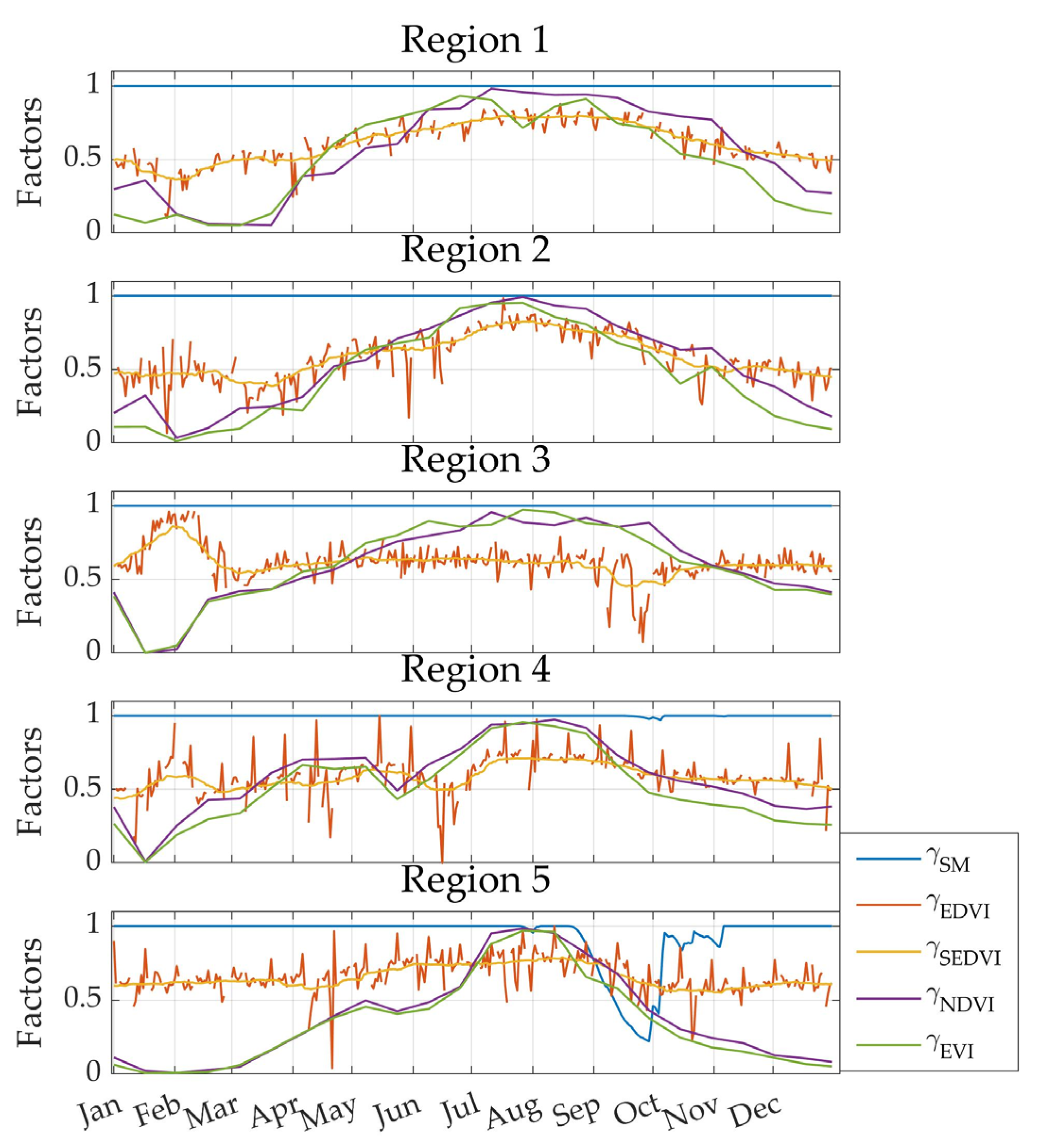
2.3. EDVI, EDVI Factor and Optical VI Factors
2.4. MEGAN Simulations
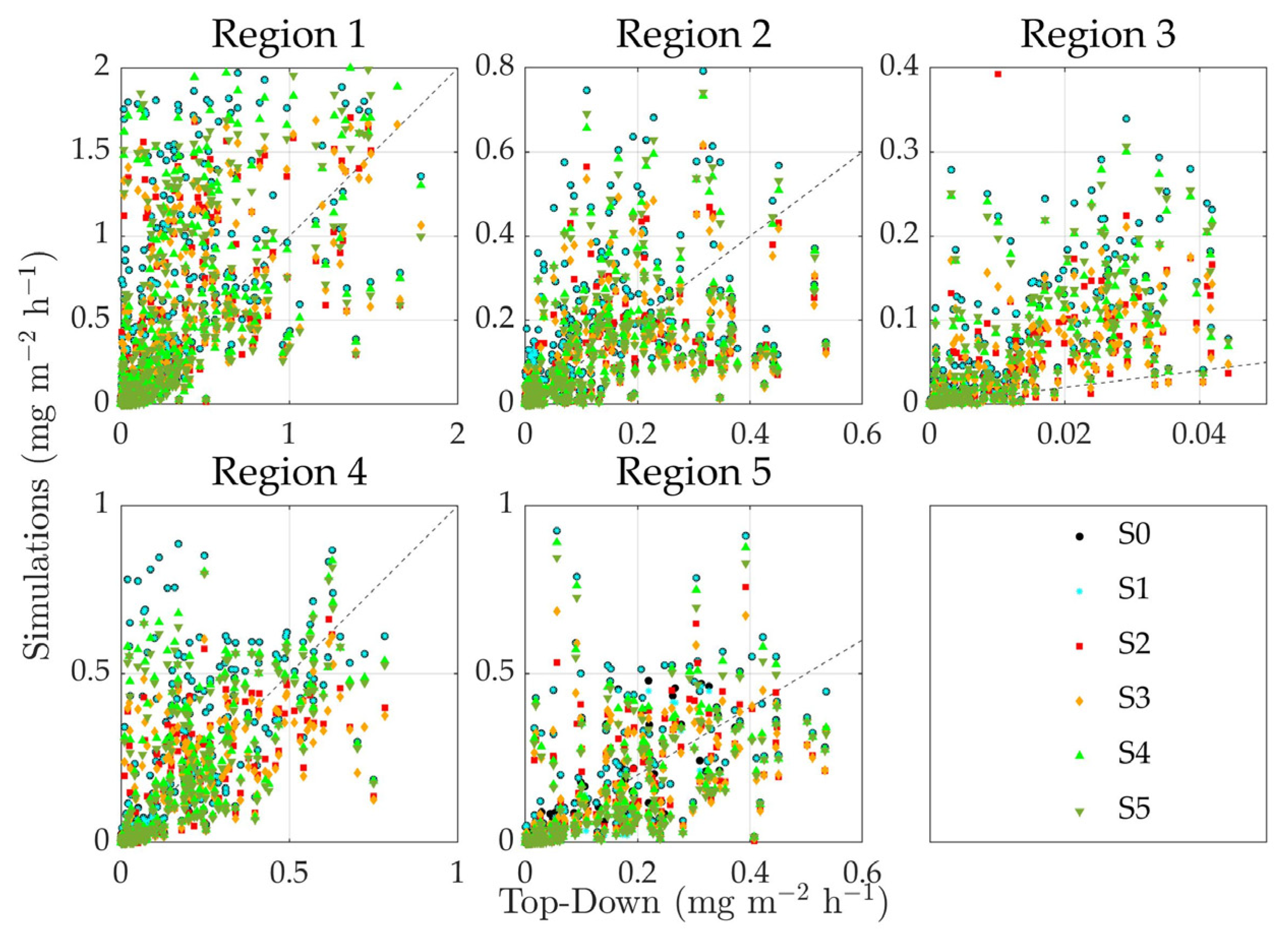
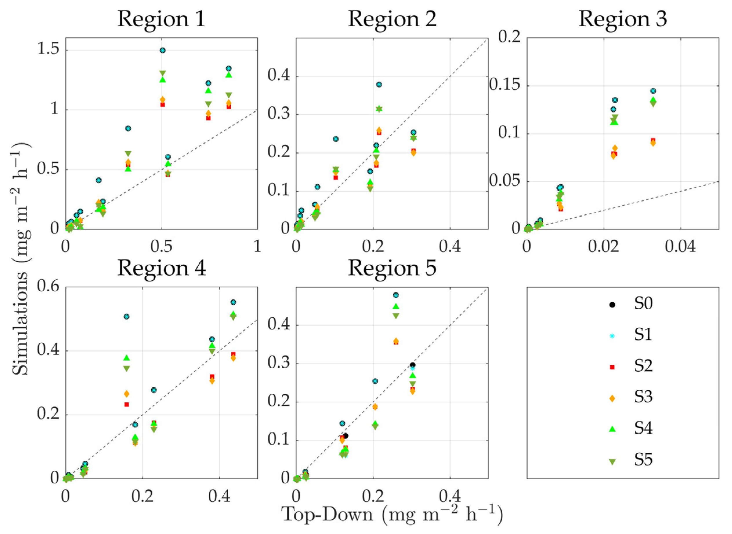
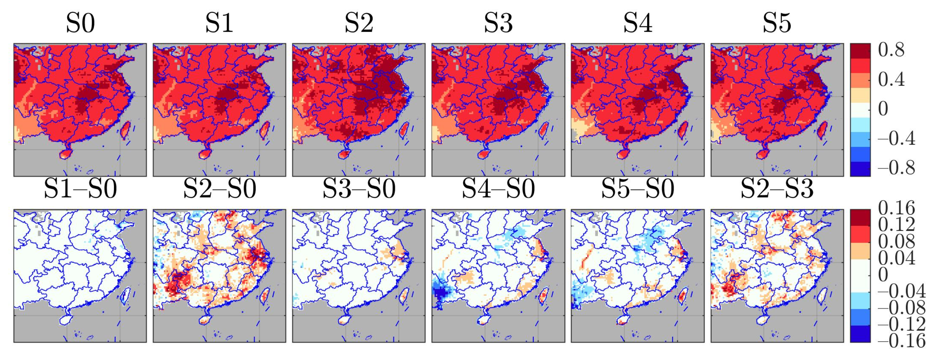
3. Results
4. Discussion
5. Conclusions
Author Contributions
Funding
Institutional Review Board Statement
Informed Consent Statement
Data Availability Statement
Acknowledgments
Conflicts of Interest
Appendix A. Effects of Winter Snow on Vegetation Indices

References
- Churkina, G.; Kuik, F.; Bonn, B.; Lauer, A.; Grote, R.; Tomiak, K.; Butler, T.M. Effect of VOC Emissions from Vegetation on Air Quality in Berlin during a Heatwave. Environ. Sci. Technol. 2017, 51, 6120–6130. [Google Scholar] [CrossRef] [Green Version]
- Pang, X.; Mu, Y.; Zhang, Y.; Lee, X.; Yuan, J. Contribution of isoprene to formaldehyde and ozone formation based on its oxidation products measurement in Beijing, China. Atmos. Environ. 2009, 43, 2142–2147. [Google Scholar] [CrossRef]
- Sun, J.; Wu, F.; Hu, B.; Tang, G.; Zhang, J.; Wang, Y. VOC characteristics, emissions and contributions to SOA formation during hazy episodes. Atmos. Environ. 2016, 141, 560–570. [Google Scholar] [CrossRef]
- Pike, R.C.; Young, P.J. How plants can influence tropospheric chemistry: The role of isoprene emissions from the biosphere. Weather 2009, 64, 332–336. [Google Scholar] [CrossRef] [Green Version]
- Ying, Q.; Li, J.; Kota, S.H. Significant Contributions of Isoprene to Summertime Secondary Organic Aerosol in Eastern United States. Environ. Sci. Technol. 2015, 49, 7834–7842. [Google Scholar] [CrossRef] [PubMed]
- Nakashima, Y.; Tsurumaru, H.; Imamura, T.; Bejan, I.; Wenger, J.C.; Kajii, Y. Total OH reactivity measurements in laboratory studies of the photooxidation of isoprene. Atmos. Environ. 2012, 62, 243–247. [Google Scholar] [CrossRef]
- Sommariva, R.; Kramer, L.J.; Crilley, L.R.; Alam, M.S.; Bloss, W.J. An instrument for in situ measurement of total ozone reactivity. Atmos. Meas. Tech. 2020, 13, 1655–1670. [Google Scholar] [CrossRef]
- Matsumoto, J. Measurements of total ozone reactivity in a suburban forest in Japan. Atmos. Environ. 2021, 246, 117990. [Google Scholar] [CrossRef]
- Liu, Y.; Brito, J.; Dorris, M.R.; Rivera-Rios, J.C.; Seco, R.; Bates, K.H.; Artaxo, P.; Duvoisin, S.; Keutsch, F.N.; Kim, S.; et al. Isoprene photochemistry over the Amazon rainforest. Proc. Natl. Acad. Sci. USA 2016, 113, 6125–6130. [Google Scholar] [CrossRef] [Green Version]
- Silver, G.M.; Fall, R. Characterization of Aspen Isoprene Synthase, an Enzyme Responsible for Leaf Isoprene Emission to the Atmosphere. J. Biol. Chem. 1995, 270, 13010–13016. [Google Scholar] [CrossRef] [Green Version]
- Schnitzler, J.P.; Arenz, R.; Steinbrecher, R.; Lehning, A. Characterization of an Isoprene Synthase from Leaves of Quercus petraea (Mattuschka) Liebl. Bot. Acta 1996, 109, 216–221. [Google Scholar] [CrossRef]
- Sharkey, T.D.; Singsaas, E.L. Why plants emit isoprene. Nature 1995, 374, 769. [Google Scholar] [CrossRef]
- Singsaas, E.L.; Lerdau, M.; Winter, K.; Sharkey, T.D. Isoprene Increases Thermotolerance of Isoprene-Emitting Species. Plant Physiol. 1997, 115, 1413. [Google Scholar] [CrossRef] [Green Version]
- Guenther, A.; Hewitt, C.N.; Erickson, D.; Fall, R.; Geron, C.; Graedel, T.; Harley, P.; Klinger, L.; Lerdau, M.; McKay, W.A.; et al. A global model of natural volatile organic compound emissions. J. Geophys. Res. Atmos. 1995, 100, 8873–8892. [Google Scholar] [CrossRef]
- Kim, J.-C. Factors controlling natural VOC emissions in a southeastern US pine forest. Atmos. Environ. 2001, 35, 3279–3292. [Google Scholar] [CrossRef]
- Peñuelas, J.; Llusià, J. The Complexity of Factors Driving Volatile Organic Compound Emissions by Plants. Biol. Plant. 2001, 44, 481–487. [Google Scholar] [CrossRef]
- Owen, S.M.; Harley, P.; Guenther, A.; Hewitt, C.N. Light dependency of VOC emissions from selected Mediterranean plant species. Atmos. Environ. 2002, 36, 3147–3159. [Google Scholar] [CrossRef] [Green Version]
- Kuhn, U.; Rottenberger, S.; Biesenthal, T.; Wolf, A.; Schebeske, G.; Ciccioli, P.; Brancaleoni, E.; Frattoni, M.; Tavares, T.M.; Kesselmeier, J. Seasonal differences in isoprene and light-dependent monoterpene emission by Amazonian tree species. Glob. Change Biol. 2004, 10, 663–682. [Google Scholar] [CrossRef]
- Tarvainen, V.; Hakola, H.; Hellén, H.; Bäck, J.; Hari, P.; Kulmala, M. Temperature and light dependence of the VOC emissions of Scots pine. Atmos. Chem. Phys. 2005, 5, 989–998. [Google Scholar] [CrossRef] [Green Version]
- Sharkey, T.D.; Loreto, F. Water stress, temperature, and light effects on the capacity for isoprene emission and photosynthesis of kudzu leaves. Oecologia 1993, 95, 328–333. [Google Scholar] [CrossRef]
- Peñuelas, J.; Filella, I.; Seco, R.; Llusià, J. Increase in isoprene and monoterpene emissions after re-watering of droughted Quercus ilex seedlings. Biol. Plant. 2009, 53, 351–354. [Google Scholar] [CrossRef]
- Guidolotti, G.; Calfapietra, C.; Loreto, F. The relationship between isoprene emission, CO2 assimilation and water use efficiency across a range of poplar genotypes. Physiol. Plant. 2011, 142, 297–304. [Google Scholar] [CrossRef] [PubMed]
- Brilli, F.; Tsonev, T.; Mahmood, T.; Velikova, V.; Loreto, F.; Centritto, M. Ultradian variation of isoprene emission, photosynthesis, mesophyll conductance, and optimum temperature sensitivity for isoprene emission in water-stressed Eucalyptus citriodora saplings. J. Exp. Bot. 2013, 64, 519–528. [Google Scholar] [CrossRef] [PubMed] [Green Version]
- Guenther, A.; Zimmerman, P.; Wildermuth, M. Natural volatile organic compound emission rate estimates for U.S. woodland landscapes. Atmos. Environ. 1994, 28, 1197–1210. [Google Scholar] [CrossRef] [Green Version]
- Kesselmeier, J.; Kuhn, U.; Wolf, A.; Andreae, M.O.; Ciccioli, P.; Brancaleoni, E.; Frattoni, M.; Guenther, A.; Greenberg, J.; De Castro Vasconcellos, P.; et al. Atmospheric volatile organic compounds (VOC) at a remote tropical forest site in central Amazonia. Atmos. Environ. 2000, 34, 4063–4072. [Google Scholar] [CrossRef] [Green Version]
- Sharkey, T.D.; Wiberley, A.E.; Donohue, A.R. Isoprene Emission from Plants: Why and How. Ann. Bot. 2008, 101, 5–18. [Google Scholar] [CrossRef] [Green Version]
- Alves, E.G.; Harley, P.; de Carvalho Gonçalves, J.F.; da Silva Moura, C.E.; Jardine, K. Effects of light and temperature on isoprene emission at different leaf developmental stages of eschweilera coriacea in central Amazon. Acta Amaz. 2014, 44, 9–18. [Google Scholar] [CrossRef]
- Guenther, A.; Karl, T.; Harley, P.; Wiedinmyer, C.; Palmer, P.I.; Geron, C. Estimates of global terrestrial isoprene emissions using MEGAN (Model of Emissions of Gases and Aerosols from Nature). Atmos. Chem. Phys. 2006, 6, 3181–3210. [Google Scholar] [CrossRef] [Green Version]
- Lathière, J.; Hauglustaine, D.A.; Friend, A.D.; De Noblet-Ducoudré, N.; Viovy, N.; Folberth, G.A. Impact of climate variability and land use changes on global biogenic volatile organic compound emissions. Atmos. Chem. Phys. 2006, 6, 2129–2146. [Google Scholar] [CrossRef] [Green Version]
- Müller, J.F.; Stavrakou, T.; Wallens, S.; De Smedt, I.; Van Roozendael, M.; Potosnak, M.J.; Rinne, J.; Munger, B.; Goldstein, A.; Guenther, A.B. Global isoprene emissions estimated using MEGAN, ECMWF analyses and a detailed canopy environment model. Atmos. Chem. Phys. 2008, 8, 1329–1341. [Google Scholar] [CrossRef] [Green Version]
- Levis, S.; Wiedinmyer, C.; Bonan, G.B.; Guenther, A. Simulating biogenic volatile organic compound emissions in the Community Climate System Model. J. Geophys. Res. Atmos. 2003, 108, 4659. [Google Scholar] [CrossRef] [Green Version]
- Abbot Dorian, S.; Palmer Paul, I.; Martin Randall, V.; Chance Kelly, V.; Jacob Daniel, J.; Guenther, A. Seasonal and interannual variability of North American isoprene emissions as determined by formaldehyde column measurements from space. Geophys. Res. Lett. 2003, 30, 111. [Google Scholar] [CrossRef] [Green Version]
- Millet, D.B.; Jacob, D.J.; Turquety, S.; Hudman, R.C.; Wu, S.; Fried, A.; Walega, J.; Heikes, B.G.; Blake, D.R.; Singh, H.B.; et al. Formaldehyde distribution over North America: Implications for satellite retrievals of formaldehyde columns and isoprene emission. J. Geophys. Res. Atmos. 2006, 111, D24S02. [Google Scholar] [CrossRef] [Green Version]
- Palmer, P.I.; Jacob, D.J.; Fiore, A.M.; Martin, R.V.; Chance, K.; Kurosu, T.P. Mapping isoprene emissions over North America using formaldehyde column observations from space. J. Geophys. Res. Atmos. 2003, 108, 4180. [Google Scholar] [CrossRef] [Green Version]
- Palmer, P.I.; Abbot, D.S.; Fu, T.-M.; Jacob, D.J.; Chance, K.; Kurosu, T.P.; Guenther, A.; Wiedinmyer, C.; Stanton, J.C.; Pilling, M.J.; et al. Quantifying the seasonal and interannual variability of North American isoprene emissions using satellite observations of the formaldehyde column. J. Geophys. Res. Atmos. 2006, 111, D12315. [Google Scholar] [CrossRef] [Green Version]
- Shim, C.; Wang, Y.; Choi, Y.; Palmer, P.I.; Abbot, D.S.; Chance, K. Constraining global isoprene emissions with Global Ozone Monitoring Experiment (GOME) formaldehyde column measurements. J. Geophys. Res. Atmos. 2005, 110, 0148–0227. [Google Scholar] [CrossRef]
- Barkley, M.P.; Palmer, P.I.; Kuhn, U.; Kesselmeier, J.; Chance, K.; Kurosu, T.P.; Martin, R.V.; Helmig, D.; Guenther, A. Net ecosystem fluxes of isoprene over tropical South America inferred from Global Ozone Monitoring Experiment (GOME) observations of HCHO columns. J. Geophys. Res. Atmos. 2008, 113, D20304. [Google Scholar] [CrossRef] [Green Version]
- Millet, D.B.; Jacob, D.J.; Boersma, K.F.; Fu, T.-M.; Kurosu, T.P.; Chance, K.; Heald, C.L.; Guenther, A. Spatial distribution of isoprene emissions from North America derived from formaldehyde column measurements by the OMI satellite sensor. J. Geophys. Res. Atmos. 2008, 113, D02307. [Google Scholar] [CrossRef]
- Marais, E.A.; Jacob, D.J.; Guenther, A.; Chance, K.; Kurosu, T.P.; Murphy, J.G.; Reeves, C.E.; Pye, H.O.T. Improved model of isoprene emissions in Africa using Ozone Monitoring Instrument (OMI) satellite observations of formaldehyde: Implications for oxidants and particulate matter. Atmos. Chem. Phys. 2014, 14, 7693–7703. [Google Scholar] [CrossRef] [Green Version]
- De Smedt, I.; Stavrakou, T.; Hendrick, F.; Danckaert, T.; Vlemmix, T.; Pinardi, G.; Theys, N.; Lerot, C.; Gielen, C.; Vigouroux, C.; et al. Diurnal, seasonal and long-term variations of global formaldehyde columns inferred from combined OMI and GOME-2 observations. Atmos. Chem. Phys. 2015, 15, 12519–12545. [Google Scholar] [CrossRef] [Green Version]
- Stavrakou, T.; Müller, J.F.; Bauwens, M.; De Smedt, I.; Van Roozendael, M.; De Mazière, M.; Vigouroux, C.; Hendrick, F.; George, M.; Clerbaux, C.; et al. How consistent are top-down hydrocarbon emissions based on formaldehyde observations from GOME-2 and OMI? Atmos. Chem. Phys. 2015, 15, 11861–11884. [Google Scholar] [CrossRef] [Green Version]
- Monson, R.K.; Fall, R. Isoprene Emission from Aspen Leaves. Plant Physiol. 1989, 90, 267. [Google Scholar] [CrossRef] [PubMed] [Green Version]
- de Souza, V.F.; Niinemets, Ü.; Rasulov, B.; Vickers, C.E.; Duvoisin Júnior, S.; Araújo, W.L.; de Carvalho Gonçalves, J.F. Alternative Carbon Sources for Isoprene Emission. Trends Plant Sci. 2018, 23, 1081–1101. [Google Scholar] [CrossRef] [PubMed]
- Pegoraro, E.; Rey, A.; Bobich, E.G.; Barron-Gafford, G.; Grieve, K.A.; Malhi, Y.; Murthy, R. Effect of elevated CO2 concentration and vapour pressure deficit on isoprene emission from leaves of Populus deltoides during drought. Funct. Plant Biol. 2004, 31, 1137–1147. [Google Scholar] [CrossRef] [Green Version]
- Guenther, A.B.; Jiang, X.; Heald, C.L.; Sakulyanontvittaya, T.; Duhl, T.; Emmons, L.K.; Wang, X. The Model of Emissions of Gases and Aerosols from Nature version 2.1 (MEGAN2.1): An extended and updated framework for modeling biogenic emissions. Geosci. Model Dev. 2012, 5, 1471–1492. [Google Scholar] [CrossRef] [Green Version]
- Llusià, J.; Peñuelas, J. Changes in terpene content and emission in potted Mediterranean woody plants under severe drought. Can. J. Bot. 1998, 76, 1366–1373. [Google Scholar] [CrossRef]
- Geron, C.; Owen, S.; Guenther, A.; Greenberg, J.; Rasmussen, R.; Hui Bai, J.; Li, Q.-J.; Baker, B. Volatile organic compounds from vegetation in southern Yunnan Province, China: Emission rates and some potential regional implications. Atmos. Environ. 2006, 40, 1759–1773. [Google Scholar] [CrossRef] [Green Version]
- Sindelarova, K.; Granier, C.; Bouarar, I.; Guenther, A.; Tilmes, S.; Stavrakou, T.; Müller, J.F.; Kuhn, U.; Stefani, P.; Knorr, W. Global data set of biogenic VOC emissions calculated by the MEGAN model over the last 30 years. Atmos. Chem. Phys. 2014, 14, 9317–9341. [Google Scholar] [CrossRef] [Green Version]
- Bauwens, M.; Stavrakou, T.; Müller, J.F.; De Smedt, I.; Van Roozendael, M.; van der Werf, G.R.; Wiedinmyer, C.; Kaiser, J.W.; Sindelarova, K.; Guenther, A. Nine years of global hydrocarbon emissions based on source inversion of OMI formaldehyde observations. Atmos. Chem. Phys. 2016, 16, 10133–10158. [Google Scholar] [CrossRef] [Green Version]
- Jiang, X.; Guenther, A.; Potosnak, M.; Geron, C.; Seco, R.; Karl, T.; Kim, S.; Gu, L.; Pallardy, S. Isoprene emission response to drought and the impact on global atmospheric chemistry. Atmos. Environ. 2018, 183, 69–83. [Google Scholar] [CrossRef]
- Tingey, D.T.; Evans, R.; Gumpertz, M. Effects of environmental conditions on isoprene emission from live oak. Planta 1981, 152, 565–570. [Google Scholar] [CrossRef] [PubMed]
- Brilli, F.; Barta, C.; Fortunati, A.; Lerdau, M.; Loreto, F.; Centritto, M. Response of isoprene emission and carbon metabolism to drought in white poplar (Populus alba) saplings. New Phytol. 2007, 175, 244–254. [Google Scholar] [CrossRef] [PubMed]
- Rodríguez-Calcerrada, J.; Buatois, B.; Chiche, E.; Shahin, O.; Staudt, M. Leaf isoprene emission declines in Quercus pubescens seedlings experiencing drought—Any implication of soluble sugars and mitochondrial respiration? Environ. Exp. Bot. 2013, 85, 36–42. [Google Scholar] [CrossRef]
- Henrot, A.J.; Stanelle, T.; Schröder, S.; Siegenthaler, C.; Taraborrelli, D.; Schultz, M.G. Implementation of the MEGAN (v2.1) biogenic emission model in the ECHAM6-HAMMOZ chemistry climate model. Geosci. Model Dev. 2017, 10, 903–926. [Google Scholar] [CrossRef] [Green Version]
- Otu-Larbi, F.; Bolas, C.G.; Ferracci, V.; Staniaszek, Z.; Jones, R.L.; Malhi, Y.; Harris, N.R.P.; Wild, O.; Ashworth, K. Modelling the effect of the 2018 summer heatwave and drought on isoprene emissions in a UK woodland. Glob. Change Biol. 2019, 26, 2320–2335. [Google Scholar] [CrossRef]
- Plaza, J.; Núñez, L.; Pujadas, M.; Pérez-Pastor, R.; Bermejo, V.; García-Alonso, S.; Elvira, S. Field monoterpene emission of Mediterranean oak (Quercus ilex) in the central Iberian Peninsula measured by enclosure and micrometeorological techniques: Observation of drought stress effect. J. Geophys. Res. Atmos. 2005, 110, D03303. [Google Scholar] [CrossRef]
- Pegoraro, E.; Rey, A.N.A.; Abrell, L.; Van Haren, J.; Lin, G. Drought effect on isoprene production and consumption in Biosphere 2 tropical rainforest. Glob. Change Biol. 2006, 12, 456–469. [Google Scholar] [CrossRef]
- Pegoraro, E.; Rey, A.; Greenberg, J.; Harley, P.; Grace, J.; Malhi, Y.; Guenther, A. Effect of drought on isoprene emission rates from leaves of Quercus virginiana Mill. Atmos. Environ. 2004, 38, 6149–6156. [Google Scholar] [CrossRef] [Green Version]
- Kalapos, T. Leaf water potential-leaf water deficit relationship for ten species of a semiarid grassland community. Plant Soil 1994, 160, 105–112. [Google Scholar] [CrossRef]
- Min, Q.; Lin, B. Determination of spring onset and growing season leaf development using satellite measurements. Remote Sens. Environ. 2006, 104, 96–102. [Google Scholar] [CrossRef]
- Li, R.; Min, Q.; Lin, B. Estimation of evapotranspiration in a mid-latitude forest using the Microwave Emissivity Difference Vegetation Index (EDVI). Remote Sens. Environ. 2009, 113, 2011–2018. [Google Scholar] [CrossRef]
- Zhang, Y.; Li, R.; Min, Q.; Bo, H.; Fu, Y.; Wang, Y.; Gao, Z. The Controlling Factors of Atmospheric Formaldehyde (HCHO) in Amazon as Seen From Satellite. Earth Space Sci. 2019, 6, 959–971. [Google Scholar] [CrossRef] [Green Version]
- Dy, C.Y.; Fung, J.C.H. Updated global soil map for the Weather Research and Forecasting model and soil moisture initialization for the Noah land surface model. J. Geophys. Res. Atmos. 2016, 121, 8777–8800. [Google Scholar] [CrossRef]
- Du, Q.; Zhao, C.; Zhang, M.; Dong, X.; Chen, Y.; Liu, Z.; Hu, Z.; Zhang, Q.; Li, Y.; Yuan, R.; et al. Modeling diurnal variation of surface PM2.5 concentrations over East China with WRF-Chem: Impacts from boundary-layer mixing and anthropogenic emission. Atmos. Chem. Phys. 2020, 20, 2839–2863. [Google Scholar] [CrossRef] [Green Version]
- Hu, J.; Fu, Y.; Zhang, P.; Min, Q.; Gao, Z.; Wu, S.; Li, R. Satellite Retrieval of Microwave Land Surface Emissivity under Clear and Cloudy Skies in China Using Observations from AMSR-E and MODIS. Remote Sens. 2021, 13, 3980. [Google Scholar] [CrossRef]
- Min, Q.; Lin, B. Remote sensing of evapotranspiration and carbon uptake at Harvard Forest. Remote Sens. Environ. 2006, 100, 379–387. [Google Scholar] [CrossRef] [Green Version]
- Li, R.; Wang, Y.; Hu, J.; Wang, Y.; Min, Q.; Bergeron, Y.; Valeria, O.; Gao, Z.; Liu, J.; Fu, Y. Spatiotemporal Variations of Satellite Microwave Emissivity Difference Vegetation Index in China Under Clear and Cloudy Skies. Earth Space Sci. 2020, 7, e2020EA001145. [Google Scholar] [CrossRef] [Green Version]
- Zheng, Y.; Unger, N.; Tadić, J.M.; Seco, R.; Guenther, A.B.; Barkley, M.P.; Potosnak, M.J.; Murray, L.T.; Michalak, A.M.; Qiu, X.; et al. Drought impacts on photosynthesis, isoprene emission and atmospheric formaldehyde in a mid-latitude forest. Atmos. Environ. 2017, 167, 190–201. [Google Scholar] [CrossRef] [Green Version]
- Bai, J.; Baker, B.; Liang, B.; Greenberg, J.; Guenther, A. Isoprene and monoterpene emissions from an Inner Mongolia grassland. Atmos. Environ. 2006, 40, 5753–5758. [Google Scholar] [CrossRef] [Green Version]
- Klinger, L.F.; Li, Q.J.; Guenther, A.B.; Greenberg, J.P.; Baker, B.; Bai, J.H. Assessment of volatile organic compound emissions from ecosystems of China. J. Geophys. Res. Atmos. 2002, 107, ACH 16-11–ACH 16-21. [Google Scholar] [CrossRef]
- Wijewardana, C.; Alsajri, F.A.; Irby, J.T.; Krutz, L.J.; Golden, B.; Henry, W.B.; Gao, W.; Reddy, K.R. Physiological assessment of water deficit in soybean using midday leaf water potential and spectral features. J. Plant Interact. 2019, 14, 533–543. [Google Scholar] [CrossRef] [Green Version]
- Zhang, Y.; Zhou, S.; Gentine, P.; Xiao, X. Can vegetation optical depth reflect changes in leaf water potential during soil moisture dry-down events? Remote Sens. Environ. 2019, 234, 111451. [Google Scholar] [CrossRef]
- Shuai, J.; Zhang, Z.; Tao, F.; Shi, P. How ENSO affects maize yields in China: Understanding the impact mechanisms using a process-based crop model. Int. J. Climatol. 2016, 36, 424–438. [Google Scholar] [CrossRef]
- Barkley, M.P.; Smedt, I.D.; Van Roozendael, M.; Kurosu, T.P.; Chance, K.; Arneth, A.; Hagberg, D.; Guenther, A.; Paulot, F.; Marais, E.; et al. Top-down isoprene emissions over tropical South America inferred from SCIAMACHY and OMI formaldehyde columns. J. Geophys. Res. Atmos. 2013, 118, 6849–6868. [Google Scholar] [CrossRef] [Green Version]


| Class | Name | Wilting Point θw (m3/m3) |
|---|---|---|
| 1 | Sand | 0.01 |
| 2 | Loamy Sand | 0.028 |
| 3 | Sandy Loam | 0.047 |
| 4 | Silt Loam | 0.084 |
| 5 | Silt | 0.061 |
| 6 | Loam | 0.066 |
| 7 | Sandy Clay Loam | 0.069 |
| 8 | Silt Clay Loam | 0.120 |
| 9 | Clay Loam | 0.103 |
| 10 | Sandy Clay | 0.100 |
| 11 | Silty Clay | 0.126 |
| 12 | Clay | 0.138 |
| 13 | Organic Matter | 0.066 |
| 14 | Water | - |
| 15 | Bedrock | 0.006 |
| 16 | Other | 0.028 |
| Class | Plant Functional Type |
|---|---|
| 1 | Needleleaf Evergreen Temperate Tree |
| 2 | Needleleaf Deciduous Boreal Tree |
| 3 | Needleleaf Evergreen Boreal Tree |
| 4 | Broadleaf Evergreen Tropical Tree |
| 5 | Broadleaf Evergreen Temperate Tree |
| 6 | Broadleaf Deciduous Tropical Tree |
| 7 | Broadleaf Deciduous Temperate Tree |
| 8 | Broadleaf Deciduous Boreal Tree |
| 9 | Broadleaf Evergreen Temperate Shrub |
| 10 | Broadleaf Deciduous Temperate Shrub |
| 11 | Broadleaf Deciduous Boreal Shrub |
| 12 | Arctic C3 Grass |
| 13 | Cool C3 Grass |
| 14 | Warm C3 Grass |
| 15 | Crop |
| 16 | Corn |
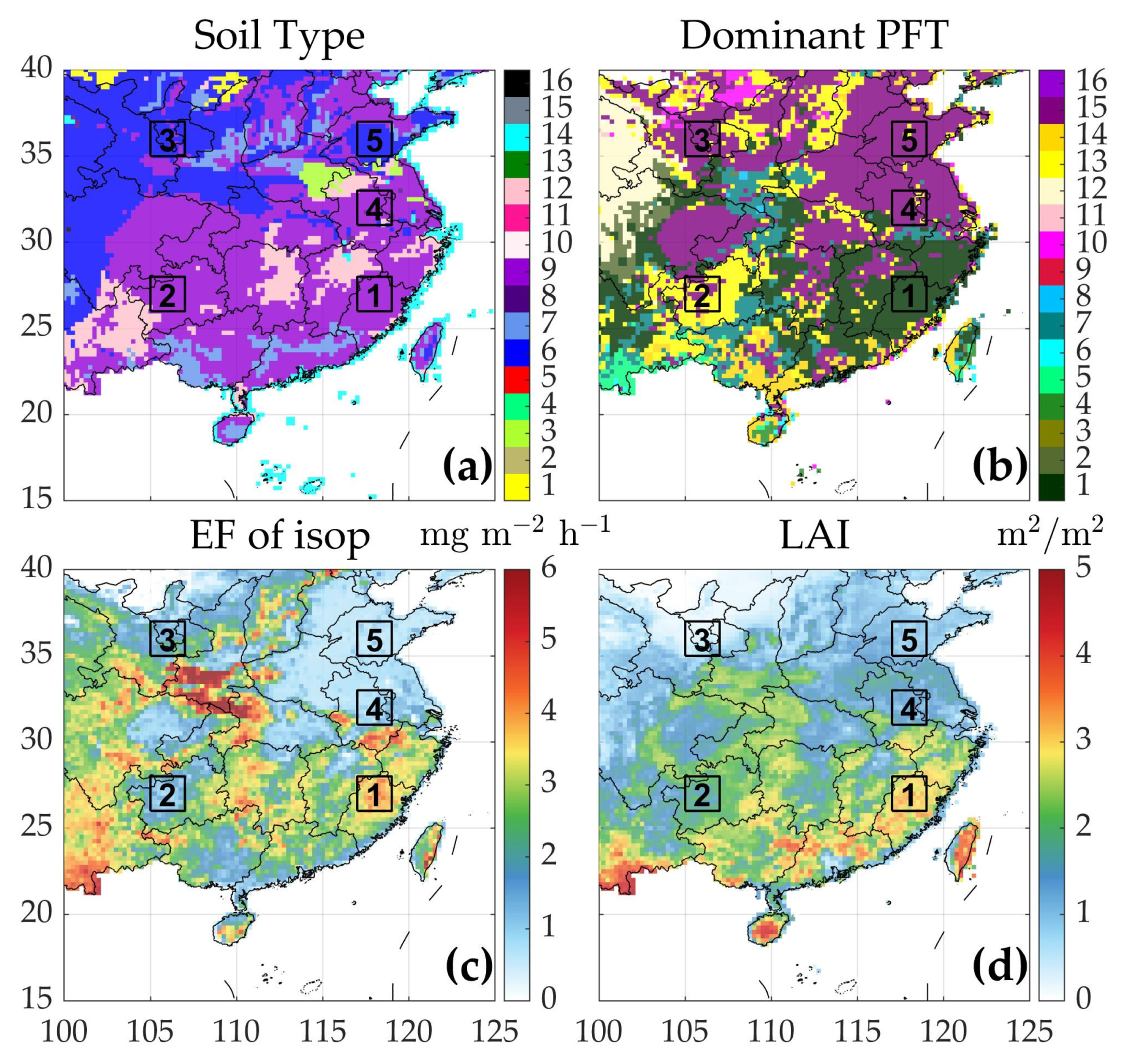
| Region | Latitude | Longitude | PFT | Soil | EF (mg m−2 h−1) |
|---|---|---|---|---|---|
| 1 | 27 | 118 | 1 (58.3%) 7 (27.4%) | 9 (100%) | 3.7 |
| 2 | 27 | 106 | 13 (42.4%) 15 (36.2%) | 9 (100%) | 1.4 |
| 3 | 36 | 106 | 15 (46.0%) 13 (10.3%) | 6 (87.5%) 9 (12.5%) | 1.7 |
| 4 | 32 | 118 | 15 (47.9%) 13 (23.8%) | 9 (92.2%) 8 (3.1%) | 1.0 |
| 5 | 36 | 118 | 15 (47.9%) 13 (22.2%) | 6 (82.8%) 9 (14.1%) | 0.8 |
| Region | Statistics | S0 | S1 | S2 | S3 | S4 | S5 |
|---|---|---|---|---|---|---|---|
| 1 | CORR | 0.62 | 0.62 | 0.66 | 0.65 | 0.66 | 0.64 |
| Bias | 0.255 | 0.255 | 0.085 | 0.101 | 0.142 | 0.126 | |
| RMSE | 0.477 | 0.477 | 0.350 | 0.363 | 0.420 | 0.415 | |
| 2 | CORR | 0.55 | 0.55 | 0.63 | 0.59 | 0.60 | 0.59 |
| Bias | 0.031 | 0.031 | −0.013 | −0.010 | 0.000 | −0.004 | |
| RMSE | 0.133 | 0.133 | 0.101 | 0.106 | 0.115 | 0.116 | |
| 3 | CORR | 0.67 | 0.67 | 0.61 | 0.67 | 0.66 | 0.67 |
| Bias | 0.034 | 0.034 | 0.017 | 0.018 | 0.028 | 0.029 | |
| RMSE | 0.061 | 0.061 | 0.039 | 0.035 | 0.054 | 0.054 | |
| 4 | CORR | 0.71 | 0.71 | 0.81 | 0.74 | 0.74 | 0.74 |
| Bias | 0.045 | 0.045 | −0.019 | −0.018 | 0.013 | 0.006 | |
| RMSE | 0.162 | 0.162 | 0.101 | 0.114 | 0.138 | 0.134 | |
| 5 | CORR | 0.72 | 0.70 | 0.74 | 0.72 | 0.69 | 0.69 |
| Bias | 0.021 | 0.015 | −0.008 | −0.008 | −0.005 | −0.010 | |
| RMSE | 0.122 | 0.124 | 0.094 | 0.097 | 0.113 | 0.108 |
| Region | Statistics | S0 | S1 | S2 | S3 | S4 | S5 |
|---|---|---|---|---|---|---|---|
| 1 | CORR | 0.91 | 0.91 | 0.93 | 0.93 | 0.94 | 0.90 |
| Bias | 0.255 | 0.255 | 0.087 | 0.101 | 0.141 | 0.126 | |
| RMSE | 0.306 | 0.306 | 0.171 | 0.184 | 0.254 | 0.260 | |
| 2 | CORR | 0.86 | 0.86 | 0.93 | 0.91 | 0.91 | 0.90 |
| Bias | 0.031 | 0.031 | −0.012 | −0.010 | 0.001 | −0.004 | |
| RMSE | 0.062 | 0.062 | 0.041 | 0.045 | 0.045 | 0.048 | |
| 3 | CORR | 0.99 | 0.99 | 0.99 | 0.98 | 0.99 | 0.99 |
| Bias | 0.034 | 0.034 | 0.017 | 0.018 | 0.028 | 0.029 | |
| RMSE | 0.047 | 0.047 | 0.025 | 0.025 | 0.041 | 0.041 | |
| 4 | CORR | 0.90 | 0.90 | 0.97 | 0.95 | 0.93 | 0.93 |
| Bias | 0.045 | 0.045 | −0.019 | −0.018 | 0.014 | 0.006 | |
| RMSE | 0.103 | 0.013 | 0.038 | 0.049 | 0.074 | 0.068 | |
| 5 | CORR | 0.94 | 0.92 | 0.94 | 0.94 | 0.89 | 0.89 |
| Bias | 0.021 | 0.015 | −0.007 | −0.008 | −0.005 | −0.010 | |
| RMSE | 0.065 | 0.070 | 0.039 | 0.041 | 0.065 | 0.062 |
Publisher’s Note: MDPI stays neutral with regard to jurisdictional claims in published maps and institutional affiliations. |
© 2022 by the authors. Licensee MDPI, Basel, Switzerland. This article is an open access article distributed under the terms and conditions of the Creative Commons Attribution (CC BY) license (https://creativecommons.org/licenses/by/4.0/).
Share and Cite
Zhang, Y.; Hu, J.; Gu, D.; Bo, H.; Fu, Y.; Wang, Y.; Li, R. Simulation of Isoprene Emission with Satellite Microwave Emissivity Difference Vegetation Index as Water Stress Factor in Southeastern China during 2008. Remote Sens. 2022, 14, 1740. https://doi.org/10.3390/rs14071740
Zhang Y, Hu J, Gu D, Bo H, Fu Y, Wang Y, Li R. Simulation of Isoprene Emission with Satellite Microwave Emissivity Difference Vegetation Index as Water Stress Factor in Southeastern China during 2008. Remote Sensing. 2022; 14(7):1740. https://doi.org/10.3390/rs14071740
Chicago/Turabian StyleZhang, Yuxiang, Jiheng Hu, Dasa Gu, Haixu Bo, Yuyun Fu, Yipu Wang, and Rui Li. 2022. "Simulation of Isoprene Emission with Satellite Microwave Emissivity Difference Vegetation Index as Water Stress Factor in Southeastern China during 2008" Remote Sensing 14, no. 7: 1740. https://doi.org/10.3390/rs14071740